Organic conductors in high magnetic fields:
model systems for quantum oscillations physics

Abstract

Even though organic conductors have complicated crystalline structure with low symmetry and large unit cell, band structure calculations predict multiband quasi-two dimensional electronic structure yielding very simple Fermi surface in most cases. Although few puzzling experimental results are observed, data of numerous compounds are in agreement with calculations which make them suitable systems for studying magnetic quantum oscillations in networks of orbits connected by magnetic breakdown. The state of the art of this problematics is reviewed. To cite this article: A. Audouard, J-Y. Fortin, C. R. Physique (2012).

Résumé Les conducteurs organiques sous champs magnétiques intenses : systèmes modèles pour la physique des oscillations quantiques. Bien que les conducteurs organiques présentent des structures cristallines complexes et de basse symétrie, les calculs prédisent une structure électronique multibande quasi-bi dimensionnelle conduisant généralement à une surface de Fermi très simple. Bien que quelques résultats expérimentaux déroutants soient observés, les données de nombreux composés sont en accord avec les calculs, ce qui fait de ces derniers des systèmes modèles pour la physique des oscillations quantiques dans les réseaux d’orbites couplées par la rupture magnétique. L’état de l’art de cette problématique est passée en revue. Pour citer cet article : A. Audouard, J-Y. Fortin, C. R. Physique (2012).

Physics

,

Received 1^er mars 2024; accepted after revision +++++

1 Introduction

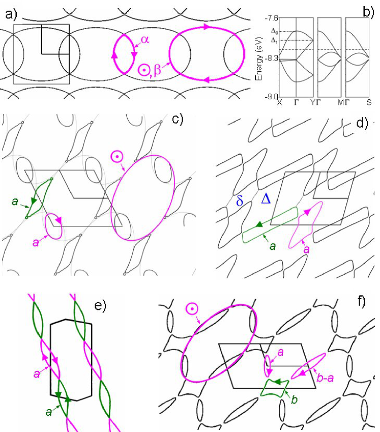
Figure 1: (Colour on-line) Fermi surface (FS) of (a) $\theta$-(ET)₄CoBr₄(C₆H₄Cl₂) [3], (c) $\beta$”-(ET)₄NH₄[Fe(C₂O₄)₃]$\cdot$(C₃H₇NO) [4], (d) (ET)₈[Hg₄Cl₁₂(C₆H₅Br)₂] [5], (e) (TMTSF)₂NO₃, in the temperature range between the anion ordering and the spin density wave condensation [6] and (f) (BEDO)₄Ni(CN)${}_{4}\cdot$4CH₃CN [7]. These FS achieve networks of hole-type (pink solid lines) and electron-type (green solid lines) orbits. Arrows indicate the quasi-particles path in magnetic field. Labels $\alpha$, $\beta$, $a$, $b$, $b-a$ and $\bigodot$ stand for few classical orbits. $\delta$ and $\Delta$ are FS pieces corresponding to forbidden orbits. (b) Energy dispersion of $\theta$-(ET)₄CoBr₄(C₆H₄Cl₂) [3].

Quasi-two dimensional (q-2D) organic metals have generally complicated crystalline structures with unit cell involving hundreds of atoms and cell parameters as large as few dozens of nm. Nevertheless, band structure calculations predict very simple Fermi surface (FS) which allow to view these compounds as model systems for quantum oscillations physics. The interplay between atomic arrangement and electronic structure is studied in Ref. [1]. Briefly, donor organic molecules such as BEDT-TTF (bis-ethylenedithio-tetrathiafulvalene, further abbreviated below as ET), BEDO-TTF (bis-ethylenedioxy-tetrathiafulvalene) or BEDT-TSF (bis-ethylenedithio-tetraselenofulvalene) build up conducting planes with various packing types, so called $\alpha$, $\beta$, $\kappa$, $etc.$ as reported in Ref. [2]. These planes are separated from each other by insulating, generally inorganic, acceptor planes. Each donor molecule bears a positive charge controlled by the anion acceptor charge and the stoichiometry. In numerous cases, which are of interest in what follows, the unit cell involves 4 donor molecules with a +1/2 charge yielding two holes per unit cell. FS of these compounds, which bears similarity with the 3D alkaline-earth metals, originates from one hole-type orbit (labeled $\bigodot$ in the following) with area equal to the first Brillouin zone (FBZ) area, that can be approximated as an ellipse in most cases. In the extended zone scheme, $\bigodot$ orbits overlap and gap opening is observed at the crossings due to lifting of degeneracy. Depending on $e.g.$ the strength of $\pi$-$\pi$ interactions between donor molecules, overlap occurs along either one or two directions, yielding networks of orbits liable to be connected to each other by magnetic breakdown (MB) in high enough magnetic field. In the first case, we deal with a linear chain of coupled 2D hole orbits. Such a network, an example of which is given in Fig. 1(a), is an experimental realization of the famous model proposed by Pippard in the early sixties to study MB [8, 9]. In the second case a 2D network of compensated orbits is observed. This latter network involves two hole-type orbits labeled $a$ and $b-a$ in Fig. 1(f) and one electron-type orbit labeled $b$. Intermediate case is depicted in Fig. 1(c) where $\bigodot$ orbits come close together in one direction. In such a case, a large gap opens around the FBZ boundary and the network is composed of one hole-type and one electron-type orbit (labeled $a$) with the same cross section. Analogous type of network is also observed in (BEDO-TTF)₂ReO${}_{4}\cdot$H₂O [1, 10] and in compounds with less trivial FS genesis due to $e.g.$ FBZ folding [5, 11] as reported in Fig. 1(d). It can also be observed in the Bechgaard salt (TMTSF)₂NO₃ (where TMTSF stands for tetramethyl-tetraselena-fulvalene). This q-1D metal at room temperature becomes q-2D at temperatures below the anion ordering (T_AO = 41 K). In-between T_AO and the spin density wave condensation temperature (T_SDW = 9.4 K), its FS achieves the linear chain of compensated orbits displayed in Fig. 1(e) [6].

Nevertheless, even not to mention structural phase transitions that can strongly affect the electronic structure, experimental data can hardly be reconciled with the calculations of Fig. 1 in few cases. This is mainly due to the extreme sensitivity of organic metals to tiny structural details [1] that can be modified by external parameters such as temperature or moderate applied pressure. In that respect, high magnetic field-induced quantum oscillations are powerful tools for the study of such FS’s. Otherwise, in the numerous cases where the calculations reported in Fig. 1 holds, MB yields oscillatory features, not predicted by the semiclassical models, the quantitative interpretation of which is still in progress.

In Section 2, we report on few examples of puzzling features of the oscillation spectra observed in organic metals with predicted FS such as those reported in Figs. 1(c) and (f). The linear chain of coupled orbits, such as that displayed in Fig. 1(a), and compensated electron-hole networks, such as reported in Fig. 1(d) and (e), are considered in Sections 3 and 4, respectively, from the viewpoint of the quantum oscillations physics in connection with MB.

2 Puzzling oscillations spectra

Shubnikov-de Haas (SdH) effect, $i.e.$ conductivity oscillations, and de Haas-van Alphen (dHvA) effect, $i.e.$ magnetization oscillations, of multiband organic metals are generally studied in the framework of the Lifshits-Kosevich model [12, 13]. For a single quadratic band $\eta$ of a q-2D system, Landau levels are given by

$$E_{\eta,n}=\hbar\omega_{\eta}(n+\frac{1}{2})+\tau_{\perp}\cos(k_{z}a_{\perp})$$ (1)

where $n$ is the Landau level index, $\omega_{\eta}=eB\cos\theta/m_{\eta}$ is the cyclotron frequency ($e=|e|$ being the electron charge), $m_{\eta}$ is the effective mass, $\tau_{\perp}$ is the interlayer energy transfer integral, $a_{\perp}$ is the distance between conducting planes and $\theta$ is the angle between the direction of the magnetic field $B$ and the normal to the conducting layers. The oscillatory part of the Kubo conductivity, in the approximation of independent collisions, and magnetization are then given by the semiclassical formulae

$$\frac{\sigma-\sigma_{0}}{2\sigma_{0}}=\frac{\Delta\sigma}{2\sigma_{0}}=\sum_{p\geq 1}\frac{(-1)^{p}}{p}J_{1}\Big{(}\frac{2\pi p\tau_{\perp}}{\hbar\omega_{\eta}}\Big{)}\Big{(}\frac{\hbar\omega_{\eta}}{\pi\tau_{\perp}}+\frac{2\pi pk_{B}T_{D}}{\tau_{\perp}}\Big{)}R_{\eta,p}\cos(2\pi p\frac{F_{\eta}}{B\cos\theta})$$ (2)

and

$$m_{osc}=-\sum_{p\geq 1}\frac{(-1)^{p}F_{\eta}}{\pi pm_{\eta}}J_{0}\Big{(}\frac{2\pi p\tau_{\perp}}{\hbar\omega_{\eta}}\Big{)}R_{\eta,p}\sin(2\pi p\frac{F_{\eta}}{B\cos\theta}),$$ (3)

respectively, for SdH and dHvA oscillations, where $\sigma_{0}=e^{2}\tau_{\perp}^{2}a_{\perp}m_{\eta}/(8\pi^{2}\hbar^{3}k_{B}T_{D})$ is the zero-field conductivity (a detailed calculation is given $e.g.$ in Refs. [14, 15, 16]), $m_{osc}$ is the oscillatory part of the magnetization [17]. $T_{D}$ is the Dingle temperature ($T_{D}$ = $\hbar$/(2$\pi k_{B}\tau)$, where $\tau$ is the relaxation time). The factor $(\hbar\omega_{\eta}/\pi\tau_{\perp}+2\pi pk_{B}T_{D}/\tau_{\perp})$ appearing in Eq. 2 is a contribution from the imaginary part of the retarded Green function $|\Im G_{\eta,n}(E)|^{2}$ coming from the Kubo formula, where $G_{\eta,n}(E)=(E-E_{\eta,n}+i\Delta_{\eta,n}(E))^{-1}$. The squared term, when expanded, has one pole of first order, giving a contribution in $1/|\Delta_{\eta,n}(E)|$, and a pole of second order, giving the second contribution equal to $2\pi p/(\hbar\omega_{\eta})$. In the usual Born approximation the imaginary part $|\Delta_{\eta,n}(E)|$ is replaced by its averaged value $<|\Delta_{\eta,n}(E)|>=\pi k_{B}T_{D}$ which defines the Dingle temperature. Moreover, the oscillating part of the self-energy, which can be included as corrections of $\pi k_{B}T_{D}$, is neglected. In the three-dimensional limit where $\tau_{perp}\gg\hbar\omega_{\eta}$, these oscillations may have significant contribution to the SdH effect. In the clean limit, $\hbar\omega_{\eta}\gg k_{B}T_{D}$ they can be discarded. The oscillation frequency $F_{\eta}=\mu m_{\eta}/(\hbar e)$ of the classical orbit $\eta$, where $\mu$ is the chemical potential, is proportional to the cross section area $A_{\eta}$ of the orbit $F_{\eta}$ = $\hbar A_{\eta}$/(2$\pi e$), which is physically the quantum flux $h/e$ through $A_{\eta}$ divided by $4\pi^{2}$. The damping factor $R_{\eta,p}$ can be factorized as

$$R_{\eta,p}(T,B)=R^{T}_{\eta,p}R^{D}_{\eta,p}R^{MB}_{\eta,p}R^{s}_{\eta,p}$$ (4)

where the thermal, Dingle, MB and spin damping factors are given by the expressions:

$$R^{T}_{\eta,p} = \frac{u_{0}Tpm_{\eta}}{B\cos\theta\sinh\Big{[}u_{0}Tpm_{\eta}/(B\cos\theta)\Big{]}},$$ (5)

$$R^{D}_{\eta,p} = \exp\Big{[}-u_{0}T_{D}pm_{\eta}/(B\cos\theta)\Big{]},$$ (6)

$$R^{MB}_{\eta,p} = (ip_{0})^{n^{t}_{\eta}}(q_{0})^{n^{r}_{\eta}},$$ (7)

$$R^{s}_{\eta,p} = \cos(\pi p\frac{g^{*}m_{\eta}}{2\cos\theta}),$$ (8)

respectively [9], where $u_{0}$ = 2$\pi^{2}m_{e}k_{B}/(e\hbar)$ = 14.694 T/K. In the following, effective masses $m_{\eta}$ are expressed in units of the electron mass $m_{e}$. Integers $n^{t}_{\eta}$ and $n^{r}_{\eta}$ are the number of MB tunnelings and reflections, respectively, encountered by the quasiparticle along its closed trajectory. $g^{*}$ is the effective Landé factor. The MB tunneling and reflection probabilities are given with a good approximation by $p_{0}$ = $\exp(-B_{0}/2B)$ and $q_{0}^{2}$ = 1 - $p_{0}^{2}$, respectively, where $B_{0}$ is the MB field. The exact semiclassical expression for the tunneling parameters can be evaluated by considering more generally the Riemann surface of the band structure [18] which is constructed from a polynomial in the complex plane $\mathbb{C}^{2}$. The singularities of this polynomial are essential in determining the genus of the Riemann surface and its homotopy group. Each element in the group is associated to a unique complex quantity $S_{\eta}$ (which is a semiclassical action on this surface) whose real part corresponds to $F_{\eta}$ and imaginary part to the MB field $B_{0}$, respectively. Even though direct application of this method is difficult in multiband systems (see few examples in Ref. [18]), it gives a nice framework and clear picture of the tunneling process.

Furthermore, FS warping can lead to beating features in the oscillatory spectra due to the interlayer transfer integral $\tau_{\perp}$ entering the Landau spectrum (see Eq. 1). Warping is accounted for by the warping factors involving $\tau_{\perp}$ in Eqs. 2 and 3. However, detailed analysis of its contribution to SdH oscillations have demonstrated that $\tau_{\perp}$ values of a few tenth of a meV, such as it is observed in $\beta$-phase compounds [19], yield oscillatory spectra that cannot be explained by the simple addition of a reduction factor [16, 20, 21, 22]. Nevertheless, $\tau_{\perp}$ is by one order of magnitude smaller in numerous q-2D organic metals, leading to warping factor values close to 1, as far as dHvA oscillations are concerned, and/or slowly varying with the magnetic field.

Finally, it should be mentioned that SdH oscillations are generally measured through interlayer magnetoresistance (R_zz) oscillations. In the case where oscillations amplitude is small compared to the background resistance R_bg, it can be assumed that -$\Delta\sigma$/$\sigma_{0}\simeq\Delta$R_zz/R_bg. Besides, contrary to magnetization which, as a thermodynamic parameter, is only sensitive to the density of states, magnetoresistance oscillations may originate from quantum interference phenomena (QI) [24, 25] as early reported for $\kappa$-(BEDT-TTF)₂Cu(NCS)₂ [26, 27, 28]. In such a case, Eqs. 2 and 5 to 8 still hold except that the effective mass entering Eqs. 5 and 6 is the difference and sum, respectively, of the two partial effective masses of each of the interferometer arms. This can lead to small and even zero-effective masses for symmetric interferometer. In such a case, oscillations are observed up to high temperature, in a range where the oscillations amplitude damping, still accounted for by $R^{D}_{\eta,p}$, is due to temperature-dependent relaxation time governed by inelastic collisions.

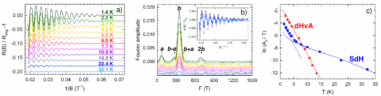
Figure 2: (Colour on-line) (a) Oscillatory part of the magnetoresistance data at ambient pressure and (b) corresponding Fourier spectra of $\beta$”-(ET)₄(H₃O)[Fe(C₂O₄)₃]$\cdot$C₆H₄Cl₂. As displayed in the inset of (b), SdH oscillations are still observed at 32 K. Curves in main panels of (a) and (b), are shifted down from each other by a constant amount. (c) Temperature dependence of the $b$ oscillations amplitude at 30 T and 34.3 T ($i.e.$ 30 T/cos(29^∘)), respectively, for SdH and dHvA data collected at ambient pressure. Solid squares are SdH data deduced from (a); solid triangles are dHvA data for $\theta$ = 29^∘. Solid lines are the best fits of the LK model assuming either only one closed orbit contributes to the amplitude (dHvA data) or the coexistence of a closed orbit and a quantum interferometer with a zero-effective mass and a temperature-dependent scattering rate (SdH data). Each of these two contributions are displayed as dashed lines. From Refs. [33, 34].

In the following, we will consider a family of organic conductors illustrating the sensitivity of the electronic structure, hence of the quantum oscillations spectra, of organic metals to small changes of the atomic structure induced by either chemical substitutions or moderate applied pressure.

Charge transfer salts with the generic formula $\beta$”-(ET)₄(A)[M(C₂O₄)₃]$\cdot$Solv (where A is a monovalent cation, M is a trivalent cation and Solv is a solvent) have raised great interest for many years [29]. These salts which share the same $\beta$” packing of the ET molecules can be either orthorhombic, in which case they are insulating, or monoclinic q-2D metals. Among these latter salts, denoted as (A, M, Solv) hereafter, many different ground-states, including normal metal, charge density wave, superconductivity, and temperature-dependent behaviours can be observed. The FS of (NH₄, Fe, C₃H₇NO) is displayed in Fig. 1(c) where the area of the compensated orbits amounts to 8.8 $\%$ of the FBZ area [4]. Analogous FS is also predicted for (H₃O, Fe, C₆H₅CN) [30]. In qualitative agreement with these calculations, only one Fourier component with frequency F = 230 T, corresponding to 6 $\%$ of the FBZ area, is observed in SdH spectra of (H₃O, Ga, C₆H₅NO₂) [31]. However, the FS of other compounds of this family can be more complicated since four frequencies corresponding to orbits area in the range 1.1 to 8.5 $\%$ of the FBZ area are observed for (H₃O, M, C₅H₅N) where M = Cr, Ga, Fe [32]. In this latter case, a density wave ground state, responsible for the observed strongly non-monotonous temperature dependence of the resistance, has been invoked to account for this discrepancy. In contrast, only two frequencies are observed for (H₃O, M, C₆H₅NO₂) where M = Cr, Ga [35]. Besides, moderate applied pressure have a drastic effect on the SdH oscillations spectra of (NH₄, Cr, C₃H₇NO). Namely, whereas up to 6 Fourier components corresponding to orbit area in the range 0.1 $\%$ to 7 $\%$ of the FBZ area are observed at ambient pressure, the spectrum simplifies under moderate pressure since only 3 components (F₁ = 68 $\pm$ 2 T, F₂ = 238 $\pm$ 4 T, F₃ = 313 $\pm$ 7 T) corresponding to orbits area in the range 1.7 $\%$ to 7.8 $\%$ of the FBZ area are observed at 1 GPa [36]. These scattered results demonstrate the sensitivity of the electronic structure of organic metals, hampering any interpretation in the framework of the band structure calculations. The last result could nevertheless be interpreted on the basis of the data in Fig. 1. Indeed, as pointed out in Ref. [4], the $\bigodot$ orbits of Fig. 1(c) may also intersect along the small axis, leading to one additional orbit as reported in Fig. 1(f). In such a case, 3 Fourier components linked by a linear combination settled by the orbits compensation, F_b = F_a + F_b-a, should be observed. This picture holds, not only for the above compound under pressure for which F₃ = F₁ + F₂ within the error bars, but also for (NH₄, Fe, C₃H₇NO) in the applied pressure range from ambient pressure to 1 GPa [37, 38] and for (H₃O, Fe, C₆H₄Cl₂) [33, 34, 39].

Further information can be obtained from the field and temperature dependence of the oscillatory spectra (see Eqs. 2 to 8). SdH and dHvA oscillations of the latter compound have been considered as displayed in Fig. 2. Whereas $a$ and $b-a$ SdH oscillations follow the LK behaviour, a kink is observed in the mass plot of the $b$ oscillations at $\sim$ 7 K. As a result, despite a rather large Dingle temperature (T_D = 4 $\pm$ 1 K), SdH oscillations are still observed at 32 K which, to our knowledge, constitutes a world record for an organic metal. In contrast, the dHvA oscillations are in agreement with the LK formula in all the explored temperature range as displayed in Fig. 2(c). Keeping in mind that dHvA oscillations are only sensitive to the density of states, it has been shown that both the field and temperature dependence of the $b$ oscillations are consistently accounted for by the coexistence of a closed $b$ orbit and a quantum interferometer with the same cross section [33, 34, 39]. Unfortunately, existence of a QI path is not consistent with the FS of Fig. 1(f) and this amazing result therefore remains unexplained.

Otherwise, the frequency F_b+a is observed both for (NH₄, Fe, C₃H₇NO) [37, 38] and (H₃O, Fe, C₆H₄Cl₂) under pressure [34, 39]. Taking into account the opposite sign of the $a$ and $b$ orbits, the $b+a$ component cannot correspond to a MB orbit [40] in the framework of the FS of Fig. 1(f). In addition, its effective mass is lower than both m_a, m_b-a and m_b which is at odds with the Falicov-Stachowiak model as well. Therefore, this component has not a semiclassical origin and can be attributed to the frequency combination phenomenon considered in the next sections.

3 The linear chain of coupled orbits

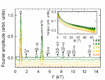
(a)

(b)

Figure 3: (Color on-line) (a) Fourier analysis in the field range 35-55.3 T of the magnetic torque data, relevant to $\theta$-(ET)₄CoBr₄(C₆H₄Cl₂), reported in the insert. Solid triangles are marks calculated with F${}_{\alpha}(\theta=0)$ = 0.944 kT and F${}_{\beta}(\theta=0)$ = 4.60 kT. Data have been shifted down from each other by a constant amount. (b) Temperature dependence (mass plot) of the 2$\alpha$ amplitude. Symbols are data deduced from torque measurements of Fig. 3(a) at 48.3 T. Solid lines are deduced from Eq. 13 with $m_{\alpha}$ = 1.81, $m_{\beta}$ = 3.52, $T_{D}$ = 0.79 K and $B_{0}$ = 35 T. Spin damping factor (see Eq. 8) is either neglected ($R^{s}_{p}$ = 1, p = 1 to 3) or accounted for by various $g^{*}$ values. All the data are normalized to their values at 12 K.

MB phenomenon has been intensively studied in 3D alkaline-earth metals over the sixties and seventies (see [9] and references therein). In order to compute MB, Pippard introduced the linear chain of coupled orbits in the early sixties [8]. The energy spectrum of this model FS, $i.e.$ the density of states in magnetic field in which all the allowed classical orbits contribute, can be computed analytically. In contrast to the semiclassical picture, a set of Landau bands broadened by coherent MB is obtained instead of discrete Landau levels, due to the traveling of quasiparticles on the non-quantized q-1D sheets of the FS. However, the Falicov-Stachowiak semiclassical model [40], based on the LK model and involving discrete Landau levels, yielded analytic tool that successfully accounted for the field and temperature dependence of the oscillations spectra of these multiband metals [9]. This success outshined the Pippard result until the discovery of frequency combinations, ’forbidden’ in the framework of the Falicov-Stachowiak model, in magnesium [41] and, later on, the experimental realization of the FS proposed by Pippard in the starring compound $\kappa$-(ET)₂Cu(NCS)₂ [42]. Many other organic metals share this FS topology, an example of which is given in Fig. 1(a). The main feature of the dHvA spectra of these compounds is the presence of the forbidden Fourier component $\beta-\alpha$ [43, 44, 45]. Furthermore, depending on the field and temperature range explored, effective masses relevant to frequency combinations linked to MB orbits can be at odds with the predictions of the Falicov-Stachowiak model, both for dHvA [44, 45] and SdH [28, 46] oscillations, even taking into account QI in the latter case. Numerical and analytical analysis of this spectrum yield, through numerical resolution, a non-LK behaviour of the oscillations amplitude [47, 48, 49]. Besides, the forbidden Fourier components observed in these compounds result not only from the formation of Landau bands but are also due to the oscillation of the chemical potential enabled by the 2D character of the FS [47, 49, 50, 51, 52, 53, 54].

Comprehensive analytical calculations of the oscillations amplitude, taking into account both coherent MB and oscillation of the chemical potential, have been reported in Refs. [55, 56] and implemented in dHvA data of $\kappa$-(ET)₂Cu(NCS)₂. However, easy to handle analytic tools necessary to quantitatively account for the experimental data were still lacking. Indeed, as pointed out in Ref. [56], the equations are complex and the data could be analyzed only numerically. In Ref. [3], a model based on the field-induced chemical potential oscillations, yielding analytical non-LK expressions for the Fourier components amplitude is proposed. This model accounts for the temperature- and field-dependent quantum oscillations spectra of the strongly two-dimensional charge transfer salt $\theta$-(ET)₄CoBr₄(C₆H₄Cl₂) with an excellent agreement. Remarkably, the unit cell of this compound involves two different donor layers [57]. One of them is insulating whereas the FS of the other, displayed in Fig. 1(a), is an illustration of the Pippard’s model. Fourier spectra of the dHvA oscillations displayed in Fig. 3(a) reveal the existence of both classical orbits $\alpha$, $\beta$, $2\beta-\alpha$ and forbidden frequencies such as $\beta-\alpha$ and its harmonics.

Considering a two band system with effective masses $m_{0(1)}$ and band extrema $\Delta_{0(1)}$, as displayed in Fig. 1(b), the grand potential $\Omega$ of a 2D slab with area $\mathcal{A}$ is given by a series of harmonics $p$ of classical frequencies $F_{\eta}$

$$\frac{\Phi_{0}}{\mathcal{A}}\frac{u_{0}}{k_{B}}\Omega(T,\mu) = \hat{\Omega}(T,\mu)=-\frac{m_{0}}{2}(\mu-\Delta_{0})^{2}-\frac{m_{1}}{2}(\mu-\Delta_{1})^{2}$$ (9)

$$+ \frac{(B\cos\theta)^{2}}{2}\sum_{p\geq 1}\sum_{\eta}\frac{C_{\eta}}{\pi^{2}p^{2}m_{\eta}}R_{\eta,p}(T,B)\cos(2\pi p\frac{F_{\eta}}{B\cos\theta}+p\varphi_{\eta})$$

in the low temperature limit and within the semiclassical approximation. The chemical potential $\mu$ and energies $\Delta_{0(1)}$ are expressed in Tesla. The universal coefficient $\Phi_{0}u_{0}/k_{B}$ (where $\Phi_{0}$ = $h/e$ is the quantum flux), in unit of which the physical quantities are expressed for simplification, is equal to $4\pi^{3}m_{e}/e^{2}\simeq 4.4\times 10^{9}$ T²m²/J. $\eta$ stands for the fundamental closed orbits that are not harmonics but can be composed of different parts of the FS thanks to MB. In particular, two fundamental orbits with frequencies $F_{\alpha}$ = $m_{1}$($\mu$ - $\Delta_{1}$) (i.e. $m_{\alpha}$ = $m_{1}$) for the smallest and $F_{\beta}$ = $m_{0}$($\mu$ - $\Delta_{0}$) + $m_{1}$($\mu$ - $\Delta_{1}$), which can be written as $F_{\beta}$ = $m_{\beta}$($\mu$ - $\Delta_{\beta}$), for the largest are defined (see Fig. 1(a)). Within this framework, $m_{0}$ + $m_{1}$ is identified with the effective mass $m_{\beta}$ of the MB orbit $\beta$. Each orbit $\eta$ has an effective mass $m_{\eta}$ and yields the frequency $F_{\eta}$ = $m_{\eta}$($\mu$ - $\Delta_{\eta}$) where $m_{\eta}$ and $\Delta_{\eta}$ are combinations of the fundamental parameters $m_{0,1}$ and $\Delta_{0,1}$. $\varphi_{\eta}$ is the phase or Maslov index determined by the number of turning points on the trajectory $\eta$. At each turning point is associated a value $\pi/2$, yielding $\varphi_{\alpha}=\varphi_{\beta}=\pi$ for orbits $\alpha$ and $\beta$ of Fig. 1(a), which is the value for a parabolic band model near the Fermi energy. For more complicated orbits, $\varphi_{\eta}$ is a multiple of $\pi$. For example the phase of the fundamental orbit $\alpha+\beta$ is $\varphi_{\alpha+\beta}=2\pi$. $C_{\eta}$ is the symmetry factor of the orbit $\eta$, which counts the number of non-equivalent possibilities for an orbit to be drawn on the FS. For example, $C_{\alpha}=C_{\beta}=C_{2\beta-\alpha}=1$ and $C_{\beta+\alpha}=2$. For a FS composed of a single orbit, $C_{\eta}=1$. We notice that frequencies $F_{\eta}$ depend explicitly on the chemical potential $\mu$. Indeed, a frequency physically represents a filling factor proportional to the orbit area in the Brillouin zone or, equivalently, the occupation number of the quasiparticles. For example, $F_{\beta}$ corresponds to the total area of the FBZ. Eq. 9 can be easily extended to more complex multiband systems. It is derived from the usual semi-classical technique using the Poisson formula applied in the case where $\hbar\omega_{c}$ is small compared to the chemical potential $\mu$ [17]. The oscillating term proportional to $B^{2}$ in Eq. 9 contains all the possible contributions of MB between the bands. In the Grand Canonical Ensemble, the chemical potential is independent of the magnetic field, leading to the expression of the magnetization $m=-\partial\hat{\Omega}/\partial(B\cos\theta)$, hence Eq. 3. In the case where the electron density is fixed, which is common in dHvA experiments, the chemical potential generally depends on the magnetic field and oscillates. These oscillations can be damped if the system is connected to a reservoir of uniform electron density [47]. The electron density per surface area $n_{e}$ is defined by d$\hat{\Omega}$/d$\mu$ = -$n_{e}$. In zero-field, Eq. 9 yields $n_{e}$ = ($m_{0}$ + $m_{1}$)$\mu_{0}$ - $m_{0}\Delta_{0}$ - $m_{1}\Delta_{1}$ where $\mu_{0}$ is the zero-field chemical potential. In the presence of a magnetic field, $\mu$ satisfies instead the following implicit equation

$$\mu=\mu_{0}-\sum_{p\geq 1}\sum_{\eta}\frac{B\cos\theta}{m_{\beta}\pi p}C_{\eta}R_{\eta,p}(T,B)\sin(\frac{2\pi pF_{\eta}}{B\cos\theta}+p\varphi_{\eta}).$$ (10)

The small oscillating part of the magnetization can be computed systematically by inserting Eq. 10 in the $\mu$-dependent terms of Eq. 9, in particular the frequencies, and computing $m=-\partial\hat{\Omega}/\partial B\cos(\theta)$. A numerical resolution of this resulting implicit equation could be done to obtain recursively the field dependence of $\mu$. Nevertheless, a more user-friendly controlled expansion in powers of the damping factors $R_{\eta,p}$ can be derived systematically at any possible order. Up to the second order, the following analytical expression is obtained for the oscillating part of the magnetization:

$$m_{osc}=-\sum_{\eta}\sum_{p\geq 1}\frac{F_{\eta}C_{\eta}}{\pi pm_{\eta}}R_{\eta,p}(T)\sin\left(\frac{2\pi pF_{\eta}}{B\cos\theta}+p\varphi_{\eta}\right)+\sum_{\eta,\eta^{\prime}}\sum_{p,p^{\prime}\geq 1}\frac{F_{\eta}C_{\eta}C_{\eta^{\prime}}}{\pi p^{\prime}m_{\beta}}R_{\eta,p}(T)R_{\eta^{\prime},p^{\prime}}(T)\times$$

$$\left[\sin\left(2\pi\frac{pF_{\eta}+p^{\prime}F_{\eta^{\prime}}}{B\cos\theta}+p\varphi_{\eta}+p^{\prime}\varphi_{\eta^{\prime}}\right)-\sin\left(2\pi\frac{pF_{\eta}-p^{\prime}F_{\eta^{\prime}}}{B\cos\theta}+p\varphi_{\eta}-p^{\prime}\varphi_{\eta^{\prime}}\right)\right]+\cdots$$ (11)

where frequencies $F_{\eta}=m_{\eta}(\mu_{0}-\Delta_{\eta})$ are evaluated at $\mu$ = $\mu_{0}$. Eq. 3 can be written as a sum of periodic functions $m_{osc}=\sum_{i}A_{i}\sin(2\pi F_{i}/(B\cos\theta))$ where the index $i$ stands for either classical orbits $\eta$ or forbidden orbits such as $\beta$ - $\alpha$. For the most relevant amplitudes, from the experimental data viewpoint, we obtain the following expressions:

$$A_{\alpha} = \frac{F_{\alpha}}{\pi m_{\alpha}}R_{\alpha,1}+\frac{F_{\alpha}}{2\pi m_{\beta}}R_{\alpha,1}R_{\alpha,2}+\frac{F_{\alpha}}{6\pi m_{\beta}}R_{\alpha,2}R_{\alpha,3}+\frac{2F_{\alpha}}{\pi m_{\beta}}R_{\beta,1}R_{\alpha+\beta,1},$$ (12)

$$A_{2\alpha} = -\frac{F_{\alpha}}{2\pi m_{\alpha}}R_{\alpha,2}+\frac{F_{\alpha}}{\pi m_{\beta}}R_{\alpha,1}^{2}-\frac{2F_{\alpha}}{3\pi m_{\beta}}R_{\alpha,1}R_{\alpha,3},$$ (13)

$$A_{\beta} = \frac{F_{\beta}}{\pi m_{\beta}}R_{\beta,1}+\frac{F_{\beta}}{2\pi m_{\beta}}R_{\beta,1}R_{\beta,2}+\frac{F_{\beta}}{6\pi m_{\beta}}R_{\beta,2}R_{\beta,3}+\frac{2F_{\beta}}{\pi m_{\beta}}R_{\beta,1}R_{\alpha+\beta,1},$$ (14)

$$A_{2\beta} = -\frac{F_{\beta}}{2\pi m_{\beta}}R_{\beta,2}+\frac{F_{\beta}}{\pi m_{\beta}}R_{\beta,1}^{2}-\frac{2F_{\beta}}{3\pi m_{\beta}}R_{\beta,1}R_{\beta,3},$$ (15)

$$A_{\beta-\alpha} = -\frac{F_{\beta-\alpha}}{\pi m_{\beta}}R_{\alpha,1}R_{\beta,1}-\frac{F_{\beta-\alpha}}{\pi m_{\beta}}R_{\alpha,2}R_{\alpha+\beta,1}-\frac{F_{\beta-\alpha}}{\pi m_{\beta}}R_{\beta,2}R_{\alpha+\beta,1},$$ (16)

$$A_{\beta+\alpha} = -\frac{2F_{\beta+\alpha}}{\pi m_{\beta+\alpha}}R_{\beta+\alpha,1}+\frac{F_{\beta+\alpha}}{\pi m_{\beta}}R_{\alpha,1}R_{\beta,1},$$ (17)

$$A_{2\beta-\alpha} = \frac{F_{2\beta-\alpha}}{\pi m_{2\beta-\alpha}}R_{2\beta-\alpha,1}+\frac{F_{2\beta-\alpha}}{2\pi m_{\beta}}R_{\alpha,1}R_{\beta,2}+\frac{F_{2\beta-\alpha}}{6\pi m_{\beta}}R_{\alpha,3}R_{\alpha+\beta,2}.$$ (18)

These equations differ from the LK model in the sense that a basic orbit such as $\alpha$, which should involve only one damping factor $A_{\alpha}=F_{\alpha}R_{\alpha}/(\pi m_{\alpha})$ according to Eq. 3, involves additional terms which are power combination of different damping factors. However, deviations from the LK behaviour due to the high order terms are significant only in the low temperature and high field ranges. This statement also stands for the classical orbit 2$\beta$-$\alpha$ since $R_{2\beta-\alpha}$ is significantly higher than the product $R_{\alpha,1}R_{\beta,2}$ (see Eq. 18). Eq. 3 bring out forbidden frequencies such as $\beta-\alpha$ (see Eq. 16). The amplitude of such Fourier component arises from the combinations of classical orbits $\alpha$ and $\beta$, hence only at the second order, through the damping factor product $R_{\alpha,1}R_{\beta,1}$. More generally, the main rule that can be derived is that products of damping factors involved at a given order represent algebraic combinations of frequencies. For example, the orbit $\beta$ in Eq. 14 can be viewed as the combinations $2\beta$ - $\beta$, or $3\beta$ - $2\beta$, yielding the factors $R_{\beta,2}R_{\beta,1}$ and $R_{\beta,3}R_{\beta,2}$, respectively, as additional factors entering the amplitude $A_{\beta}$. As a consequence, forbidden frequencies arise from the order two since they cannot be due to any single classical orbit. Algebraic sums of damping terms in Eqs. 13 and 17 may possess minus signs which account for $\pi$ dephasings, and may cancel at field and temperature values, depending strongly on the effective masses, Dingle temperature, MB field, $etc.$ as displayed in Fig. 3(b) relevant to 2$\alpha$. This point has already been reported for the second harmonic of the basic orbits both for compensated [58] and un-compensated [54] metals.

Finally, even taking into account the contribution of QI, stronger deviations from the semiclassical model are reported in the case of SdH spectra of several compounds with this FS topology [3, 47, 46]. These features are not accounted for by the above calculations which therefore requires a specific model.

4 Networks of compensated orbits

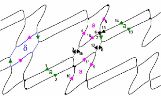
Figure 4: (Colour on-line) Forbidden (left side) and MB-induced (right side) $\delta$ orbit relevant to the Fermi surface of (ET)₈[Hg₄Cl₁₂(C₆H₅Br)₂] [5]. Numbers on the right side indicates the successive steps of the quasiparticles starting from an (arbitrary) origin marked by the open circle. Arrows mark the quasiparticles path. Pink and green arrows correspond to hole and electron parts, respectively, of the Fermi surface. Black arrows and circles mark the magnetic breakdown tunneling junctions and reflections, respectively. Taking into account the opposite sign of the compensated electron and hole basic orbits (labeled $a$), the considered MB orbit yields a frequency corresponding to the area of $\delta$.

Let us consider now the other class of FS’s, widely encountered in organic metals, which are built up with compensated electron and hole orbits (few examples are reported in Figs. 1(c)-(f)). Depending on MB gaps value, either isolated orbits, 1D or 2D networks are observed. As mentioned in Section 2, few hints of forbidden frequency combinations are observed in SdH spectra of $\beta$”-(ET)₄NH₄[Fe(C₂O₄)₃]$\cdot$C₃H₇NO. Besides, QI which requires MB gaps crossing as well, have been tentatively inferred to account for the oscillatory data of $\beta$”-(ET)₄(H₃O)[Fe(C₂O₄)₃]$\cdot$C₆H₄Cl₂ reported in Fig 2. However, to our knowledge, the only compounds studied from this viewpoint belong to the family (ET)₈[Hg₄X₁₂(C₆H₅Y)₂] (where X, Y = Cl, Br) [5, 59, 60, 61, 62, 63]. Indeed, due to moderate MB gaps, compounds with X = Cl achieves 2D networks as reported in Fig. 1(d). In addition, small scattering rate (T_D = 0.2 $\pm$ 0.2 K) is observed [61]. In line with the Falicov-Stachowiak model, Fourier components are linear combinations of the frequencies linked to the compensated closed orbits $a$ and to the ’forbidden’ orbits $\delta$ and $\Delta$ [5, 60, 61, 62]. This is the case of $e.g.$ $2a+\delta$ which is observed both in SdH and dHvA spectra. Regarding magnetoresistance, components linked to QI such as $a+\delta$ and $2a+\delta+\Delta$ are also observed in the spectra. Strictly speaking, there is no forbidden orbit in a 2D network of compensated orbits. For example, keeping in mind that electron and hole orbits have opposite signs, a MB-induced orbit with the frequency corresponding to $\delta$ can be defined for the FS of Fig. 1(d) as displayed in Fig. 4. However, according to the Falicov-Stachowiak model, its amplitude should be very small. Indeed, this orbit involves 6 MB tunnelings and 10 reflections leading to small $R^{MB}$ values (see Eq. 7). Besides, its effective mass $m_{\delta}$ should amount to 4$m_{a}$ leading to small $R^{D}$ and $R^{T}$ values, as well. In violation of these statements, ’forbidden’ orbits such as $\delta$ or $4a+\delta$, with a small effective mass ($m_{\delta}\simeq$ 0.4$m_{a}$, $m_{4a+\delta}\simeq$ 0.3$m_{a}$ [61]) and a large amplitude, are observed. As a result, these two Fourier components which should not be observed in the framework of the semiclassical model, are preponderant above few kelvins at moderate fields (see Fig. 5).

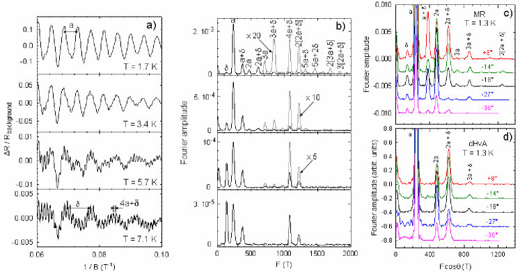
Figure 5: (Colour on-line) (a) Oscillatory part of the magnetoresistance and (b) corresponding Fourier spectra of (ET)₈[Hg₄Cl₁₂(C₆H₅Br)₂] at various temperatures [61]. Fourier spectra of (c) magnetoresistance and (d) de Haas-van Alphen oscillations for various directions of the magnetic field [62]. Data in (c) and (d) have been measured simultaneously. Labels $a$ and $\delta$ correspond to closed and forbidden orbits, respectively, depicted in Fig 1(d). Contrary to magnetoresistance oscillations spectra which exhibits forbidden frequency combinations, all the observed dHvA components are accounted for by the Falicov-Stachowiak semiclassical model.

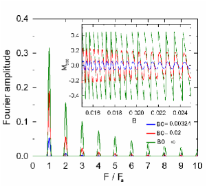
(a)

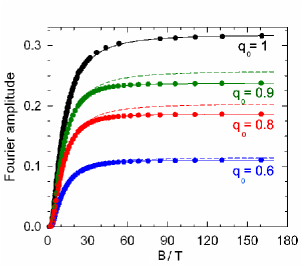
(b)

Figure 6: (Color on-line) (a) Fourier spectra of the dHvA oscillations, displayed in the insert, of a linear chain of compensated orbits, for various values of the magnetic breakdown field $B_{0}$. The data are calculated from numerical resolution of the field-dependent free energy equation with $\Delta$ = 1 and effective masses $m_{e}$ = 1 and $m_{h}$ = 2.5 (see text and Ref. [58]). $F_{a}=7/2$ is the fundamental frequency for this model. (b) $B/T$ dependence of the first harmonic amplitude $A_{a}$ for various values of the tunneling probability (hence of the magnetic field). Solid symbols come from numerical resolution of the semiclassical spectrum, which fall onto the solid lines corresponding to the Lifshits-Kosevich approximation given by Eq. 19 including contributions of zero area orbits. Dashed lines correspond to the first order term $l=1$ in Eq. 19 or equivalently to Eq. 3.

Contrary to magnetoresistance data, the whole dHvA spectra is quantitatively accounted for by the Falicov-Stachowiak model in the field range up to 28 T [62]. This latter point is at variance with the data for the linear chain of coupled orbits considered in Section 3. In order to solve this discrepancy, a linear chain of compensated orbits, $i.e.$ the 1D network which accounts for the FS in Fig. 1(e), has been considered as a first step in Refs. [58, 64]. Indeed, its energy spectrum can be easily deduced from the Pippard’s method [8]. In this model the effective masses linked to the electron $m_{e}$ and hole band $m_{h}$ are taken to be independent. For simplicity, two quadratic potentials have been considered to model the FS, i.e. quadratic functions of the quasi-momenta are assumed for the bands dispersion, as within the free-electron model in two dimensions. The bottom of the electron band is set at zero energy while the top of the hole band (inverse quadratic potential) is at $\Delta>0$, with the possibility for the quasiparticle to tunnel through the gap between two successive orbits by MB, i. e. between the pink and green parts of the FS in Fig. 1(e). Given an energy $E$, the k-space areas of the closed electron and hole orbits are respectively given by $S_{e}=2\pi m_{e}E$ and $S_{h}=2\pi m_{h}(\Delta-E)$, which are both quantized. The zero field Fermi energy $E_{F}$ is given by the condition of compensation $S_{e}(E_{F})=S_{h}(E_{F})$ or $E_{F}=[m_{h}/(m_{e}+m_{h})]\Delta$. The unique fundamental frequency of this system is therefore equal to $F_{a}=S_{e}(E_{F})/2\pi=S_{h}(E_{F})/2\pi=m_{e}m_{h}\Delta/(m_{e}+m_{h})$.

Strikingly, the field-induced chemical potential oscillation, calculated by extremizing the free energy is strongly damped compared to the uncompensated case of Section 3 [58, 64]. For this reason, Fourier amplitudes can be calculated within the LK formalism. Nevertheless, it is important to notice that, in systems with compensated bands, there is an infinite number of classical orbits contributing to any given Fourier component since a semi-classical trajectory around a successive electron and hole pockets has a zero area. Here orbits with zero area can be classified by their increasing masses $(l-1)m_{e}+(l-1)m_{h}$, where $l>$ 1 is an integer. The amplitude $A_{a}$ of the Fourier component with frequency $F_{a}$ is therefore not only dependent on the orbits composed of one electron or one hole orbit with effective mass $m_{e}$ or $m_{h}$, respectively, but also on a series of additional multiple orbits composed of $l-1$ electron and $l-1$ hole orbits plus one electron or one hole orbit, with effective mass $m_{e}(l)=lm_{e}+(l-1)m_{h}$ or $m_{h}(l)=(l-1)m_{e}+lm_{h}$, respectively. $A_{a}$ can be computed exactly in this model, within the LK theory, and is given by the expression

$$A_{a} = \frac{F_{a}}{\pi}\Big{[}\frac{q_{0}^{2}R(m_{e})}{m_{e}}+\frac{q_{0}^{2}R(m_{h})}{m_{h}}+\sum_{l\geq 2}\Big{(}\frac{R(m_{e(l)})}{m_{e}(l)}+\frac{R(m_{h(l)})}{m_{h}(l)}\Big{)}\times\sum_{n=1}^{2(l-1)}(-1)^{n}p_{0}^{2n}q_{0}^{4l-2n-2}{\mathcal{S}}(l,n)\Big{]}$$ (19)

where the combinatorial quantities can be defined by the summations

$${\mathcal{S}}(l,n)=\frac{2}{n}\sum_{i=0}^{n/2}\sum_{j=0}^{i}\sum_{k=0}^{n/2-j}\frac{(-1)^{j}}{2^{2k}}\times\left({}^{n}_{2i}\right)\left({}^{i}_{j}\right)\left({}^{n-2j}_{2k}\right)\left({}^{2k}_{k}\right)\left({}^{l+k-1}_{l-n+j+k}\right)\left({}^{l+k-2}_{l-n+j+k-1}\right).$$ (20)

These positive integers count the number of non-equivalent orbits for a given mass $m_{e(h)}(l)$ visiting $2n$ pockets on the path. Table 1 displays the numerical values of $S(l,n)$ computed directly from Eq. 20. Damping factors are given by $R(m_{i(l)})=R^{T}_{i,l}R^{D}_{i,l}R^{s}_{i,l}$, where $i=e,h$. $p_{0}$ and $q_{0}$ are the MB tunneling and reflection probabilities (see Eqs. 5 to 8). Even though the contribution of large masses is usually negligible at low field or high temperature, it can be significant in the large $B/T$ limit in which case they have to be taken into account, provided the Dingle temperature is small [58]. Indeed, the temperature dependent factors are close to unity in this limit.

Table 1: First values of the coefficients ${\mathcal{S}}(l,n)$ representing the number of non-equivalent orbits for a given mass $m_{e(h)}(l)$ with $2n$ magnetic breakdowns, $1\leq n\leq 2(l-1)$.

${}_{l}\backslash^{n}$	1	2	3	4	5	6	7	8	9	10	11	12
2	2	1
3	2	9	8	1
4	2	23	68	63	18	1
5	2	43	264	610	584	228	32	1
6	2	69	720	3080	6132	5930	2800	600	50	1
7	2	101	1600	10925	36980	66374	64952	34550	9650	1305	72	1

Technically, the summation over all the orbits with zero area is evaluated using an analogy with an Ising model on a linear chain in magnetic field. Indeed, it is useful to view each quasiparticle traveling on the linear chain represented by the FS of Fig.1(e) as a particle performing a one dimensional random walk. A set of positions on the chain $\{x_{i}\}_{i=0,2n}$ can be defined for a given periodic orbit, with boundary conditions $x_{0}=x_{2n}=0$. These coordinates take integer values (negative and positive) and define the pocket inside which the quasiparticle is located. In what follows, $x_{i}$ with $i$ even (odd) is the position of a quasiparticle in one electron (hole) band. A closed path has an even number of steps $2n$. Given $x_{i}$, the particle can also orbit a number $n_{i}\geq 0$ of times around the surface before going to the next band by MB. We can rewrite coordinates $x_{i}$ with mean of forward/backward variables $\sigma_{i}=\pm 1$ such as $x_{i}=x_{i-1}+\sigma_{i}(x_{i-1}-x_{i-2})$. Here $\sigma_{i}=1$ when the particle is going forward and $\sigma_{i}=-1$ when it is going backward. An adequate set of variables is given by $y_{i}=x_{i}-x_{i-1}=\pm 1$ which satisfy $y_{i}=\sigma_{i}y_{i-1}$ or $\sigma_{i}=y_{i}y_{i-1}$. All the possible orbits contributing with a given effective mass can then be counted by summing over all the possible $y_{i}=\pm$1 restricted to the boundary conditions. It can then be proved that this combinatorial number is equal to the partition function of an Ising model in a (complex) magnetic field and which is solvable, leading to Eq. (20). In two-dimensions, compensated networks such as the FS reported in Fig. 1(d) could also lead to non-negligible contribution of zero-area orbits, but their explicit evaluation is difficult since a similar analogy with the previous calculation would lead equivalently to the computation of the partition function for a two-dimensional Ising model in magnetic field.

The relevance of Eq. 19 is evidenced in Fig. 6(a). Oscillations data in this figure are calculated from numerical resolution of the field-dependent free energy equation given in Ref. [58]. As expected, Fourier analysis exhibits only one frequency $F_{a}$ and harmonics. Fig. 6(b) compares the temperature dependence of $A_{a}$ deduced from numerical resolution (solid symbols) to the predictions of Eq. 3, which neglects any contribution of orbits with $l>$ 1 (dashed lines). A growing discrepancy is observed as the temperature decreases, except in the absence of MB ($q_{0}$ = 1) in which case only the basic closed orbits contributes. In contrast, an excellent agreement with Eq. 19 (solid lines) is observed. Shortly speaking, at variance with uncompensated orbits networks, the LK formula accounts for the quantum oscillations in a linear chain of compensated orbits (one-dimensional network), provided the contribution of all MB orbits is taken into account for each frequency.

5 Conclusion

Although few puzzling results are observed, as reported in Section 2, numerous organic conductors achieve Fermi surfaces that can be regarded as model systems for the study of quantum oscillations in networks of orbits coupled by magnetic breakdown. Two types of networks can be distinguished, namely the linear chain of coupled orbits and the networks of compensated orbits (see few examples in Fig. 1). These networks are considered in Sections 3 and 4, respectively.

A user friendly analytical tool, taking into account the chemical potential oscillations in magnetic field, has recently been proposed to account for dHvA oscillation spectra of the linear chain of coupled orbits [3]. The main feature of the derived formulae is, besides standard Lifshits-Kosevich terms, the presence of second order corrections liable to account for the observed Fourier components that are ’forbidden’ in the framework of the semiclassical Falicov-Stachowiak model. This model has been successfully implemented in the dHvA oscillations data of $\theta$-(ET)₄CoBr₄(C₆H₄Cl₂). Obviously, this encouraging result needs to be confirmed in the case of other relevant compounds. In addition, even stronger deviations are observed for SdH spectra which are still unexplained.

Regarding compensated orbits, either one- (see Fig. 1(e)) or two-dimensional (see Fig. 1(d), (f)) networks can be observed. At variance with the above case, oscillations of the chemical potential are strongly damped in one-dimensional networks and the Lifshits-Kosevich theory applies in this case, provided multiple orbits are taken into account. Unfortunately, to our knowledge, no experimental data relevant to one-dimensional networks are available to check this result. Nevertheless, dHvA oscillations spectra of the two-dimensional network achieved by the (ET)₈[Hg₄Cl₁₂(C₆H₅Br)₂] compound are nicely accounted for by the Falicov-Stachowiak model in magnetic fields below 28 T which is in line with the above reported damping of the chemical potential oscillations. However, SdH oscillations evidences strong deviations from the Lifshits-Kosevich model, including the presence of ’forbidden’ Fourier components with high amplitude, besides the contribution of quantum interference. These results still require interpretation.

Regarding new problematics, promising perspective are brought about by organic metals with two different donors planes, few examples of which can be found in the literature. In few cases, a metal-insulator transition is observed as the temperature decreases [65, 66] suggesting two insulating planes at low temperature. Compounds with one metallic and one insulating layer with either compensated orbits [67] or, as reported in Section 3, linear chain of coupled orbits [3, 57] have also been reported. In these cases, a strongly two-dimensional behaviour is observed. More appealing case is provided by unit cell with two different metallic layers [68, 69, 70], hence with two different Fermi surfaces [69]. Such a structure could be relevant to the bilayer splitting phenomenon reported for cuprate superconductors [71] and addresses the question of a three-dimensional Fermi surface definition. To our knowledge, quantum oscillations data at high field have only been reported for $\theta$-(BEDT-TSF)₄HgBr₄(C₆H₅Cl) for which complicated spectra, with no clear frequency combinations are observed [69]. In any case, the oscillatory data cannot be interpreted on the basis of a mere addition of the contributions of the two Fermi surfaces pertaining to each of the two donors planes. Synthesis of other compounds and further experiments are needed to get a better insight on this issue.

References

- [1] R. Rousseau, M. Gener and E. Canadell, Step-by-step construction of the electronic structure of molecular conductors: conceptual aspects and applications, Adv. Func. Mater. 14 (2004) 201.
- [2] R. P. Shibaeva and E. B. Yagubskii, Molecular Conductors and Superconductors Based on Trihalides of BEDT-TTF and some of Its analogues, Chem. Rev. 104 (2004) 5347.
- [3] A. Audouard, J.-Y. Fortin, D. Vignolles, R. B. Lyubovskii, L. Drigo, F. Duc, G. V. Shilov, Géraldine Ballon, E. I. Zhilyaeva, R. N. Lyubovskaya and E. Canadell, Quantum oscillations in the linear chain of coupled orbits: the organic metal with two cation layers -(ET)4CoBr4(C6H4Cl2), arXiv:1110.3696v1.
- [4] T. G. Prokhorova, S. S. Khasanov, L. V. Zorina, L. I. Buravov, V. A. Tkacheva, A. A. Baskakov, R. B. Morgunov, M. Gener, E. Canadell, R. P. Shibaeva and E. B. Yagubskii, Molecular metals based on BEDT-TTF radical cations salts with magnetic metal oxalates as counterions: ”-(ET)4A[M(C2O4)3]DMF (A= NH, M=CrIII, FeIII), Adv. Funct. Mater. 13 (2003) 403.
- [5] D. Vignolles, A. Audouard, R. B. Lyubovskii, M. Nardone, E. Canadell and R. N. Lyubovskaya, Shubnikov-de Haas oscillations spectrum of the strongly correlated quasi-2D organic metal (BEDT-TTF)8Hg4Cl12(C6H5Br)2 under pressure, Eur. Phys. J. B, 66 (2008) 489.
- [6] W. Kang, K. Behnia, D. J rome, L. Balicas, E. Canadell, M.Ribault and J. M. Fabre, Fermi-Surface Instabilities In The Organic Conductor (TMTSF)2NO3 - High-Pressure Studies, Europhys. Lett. 29 (1995) 635.
- [7] A. D. Dubrovskii, N. G. Spitsina, L. I. Buravov, G. V. Shilov, O. A. Dyachenko, E. B. Yagubskii, V. N. Laukhin and E. Canadell, New molecular metals based on BEDO radical cation salts with the square planar Ni(CN) anion, J. Mater. Chem. 15 (2005) 1248.
- [8] A. B. Pippard, Quantization of coupled orbits in metals, Proc. Roy. Soc. (London) A270 (1962) 1.
- [9] D. Shoenberg, Magnetic Oscillations in Metals, Cambridge University Press, Cambridge, 1984.
- [10] S.S Khasanov, B.Z. Narymbetov, L.V. Zorina, L.P. Rozenberg, R.P. Shibaeva, N.D. Kushch, E.B. Yagubskii, R. Rousseau and E. Canadell, Eur. Phys. J. B 1 (1998) 419.
- [11] L. F. Veiros and E. Canadell, Characterization of the Fermi surface of BEDT-TTF4[Hg2Cl6]PhCl by electronic band structure calculations, J. Phys. I France 4 (1994) 939.
- [12] I.M. Lifschitz and A.M. Kosevich, On the theory of the de Haas-van Alphen effect for particles with an arbitrary dispersion law, Dokl. Akad. Nauk SSSR 96 (1954) 963 (in Russian).
- [13] A.M. Kosevich and I.M. Lifschitz, On the theory of magnetic susceptibility of metals at low temperatures, Zh. Eks. Teor. Fiz. 29 (1955) 730 [Sov. Phys. JETP 2 (1956) 636].
- [14] E.M. Lifshitz and L. P. Pitaevskii, Physical Kinetics: Volume 10 (Course of Theoretical Physics), Butterworth-Heinemann Ltd, Oxford 1981.
- [15] I. O. Thomas, V. V. Kabanov and A. S. Alexandrov, Phys. Rev. B 77 (2008) 075434.
- [16] P. D. Grigoriev, Theory of the Shubnikov-de Haas effect in quasi-two-dimensional metals, Phys. Rev. B 67 (2003) 144401.
- [17] E.M. Lifshitz and L. P. Pitaevskii, Statistical Physics, Part 2: Volume 9 (Course of Theoretical Physics), Butterworth-Heinemann Ltd, Oxford 1980.
- [18] J.-Y. Fortin, J. Bellissard, M. Gusmão, and T. Ziman, de Haas-van Alphen oscillations and magnetic breakdown: Semiclassical calculation of multiband orbits, Phys. Rev. B 57 (1998) 1484.
- [19] J. R. Cooper, L. Forro, B. Korin-Hamzic, M. Miljak and D. Schweitzer, Some electronic properties of the organic superconductor -(BEDT-TTF)2I3, J. Phys. France 50 (1989) 2741.
- [20] M. Kartsovnik, P. D. Grigoriev, W. Biberacher, N. D. Kushch and P. Wyder, Slow oscillations of magnetoresistance in quasi-two-dimensional metals, Phy. Rev. Lett 89 126802 (2002).
- [21] M. V. Kartsovnik, High magnetic fields: a tool for studying electronic properties of layered organic metals, Chem. Rev. 104 5737 (2004).
- [22] M. V. Kartsovnik, V. A. Pechansky, Galvanomagnetic phenomena in layered organic conductors, Low Temp. Phys. 31 (2005) 185.
- [23] J. Singleton, P. A. Goddard, A. Ardavan, N. Harrison, S. J. Blundell, J. A. Schlueter and A. M. Kini, Test for Interlayer Coherence in a Quasi-Two-Dimensional Superconductor, Phys. Rev. Lett. 88 (2002) 037001.
- [24] R. W. Stark and C. B. Friedberg, Quantum interference of electron waves in a normal metal, Phys. Rev. Lett. 26 (1971) 556.
- [25] R. W. Stark and C. B. Friedberg, Interfering electron quantum states in ultrapure magnesium, J.Low Temp. Phys. 14 (1974) 111.
- [26] J. Caulfield, J. Singleton, F.L. Pratt, M. Doporto, W. Lubczynski, W. Hayes, M. Kurmoo, P. Day, P.T.J. Hendriks and J.A.A.J. Perenboom, The effects of open sections of the Fermi surface on the physical properties of 2D organic molecular metals, Synth. Met. 61 (1993) 63.
- [27] M. V. Kartsovnik, G. Yu. Logvenov, T. Ishiguro, W. Biberacher, H. Anzai, and N. D. Kushch, Direct Observation of the Magnetic-Breakdown Induced Quantum Interference in the Quasi-Two-Dimensional Organic Metal -(BEDT-TTF)2Cu(NCS)2, Phys. Rev. Lett. 77 (1996) 2530.
- [28] N. Harrison, J. Caulfield, J. Singleton, P. H. P. Reinders, F. Herlach, W. Hayes, M. Kurmoo and P. Day, Magnetic breakdown and quantum interference in the quasi-two-dimensional superconductor -(BEDT-TTF)2Cu(NCS)2 in high magnetic fields, J. Phys.-Condens. Matter 8 5415 (1996).
- [29] E. Coronado and P. Day, Magnetic molecular conductors, Chem. Rev. 104 (2004) 5419.
- [30] M. Kurmoo, A. W. Graham, P. Day, S. J. Coles, M. B. Hursthouse, J. L. Caulfield, J. Singleton, F. L. Pratt, W. Hayes, L. Ducasse and P. Guionneau, Superconducting and semiconducting magnetic charge transfer salts: (BEDT-TTF)4AFe(C2O4).C6H5CN (A = H2O, K, NH4), J. Am. Chem. Soc. 117 (1995) 12209.
- [31] A. Bangura, A. Coldea, A. Ardavan, J. Singleton, A. Akutsu-Sato, H. Akutsu and P. Day, The effect of magnetic ions and disorder on superconducting ”-(ET)4H3O[M(C2O4)3]C6H5NO2 salts, where M = Ga and Cr, J. Phys. IV France 114 (2004) 285.
- [32] A. Coldea, A. Bangura, J. Singleton, A. Ardavan, A. Akutsu-Sato, H. Akutsu, S. S. Turner and P. Day, Fermi-surface topology and the effects of intrinsic disorder in a class of charge-transfer salts containing magnetic ions: ”-(ET)4H3O[M(C2O4)3]Y (M=Ga, Cr, Fe; Y=C5H5N), Phys. Rev. B 69 (2004) 085112.
- [33] D. Vignolles, A. Audouard, V.N. Laukhin, E. Canadell, T.G. Prokhorova and E.B. Yagubskii, Indications for the coexistence of closed orbit and quantum interferometer in ”-(ET)4(H3O)[Fe(C2O4)3]C6H4Cl2: persistence of Shubnikov-de Haas oscillations above 30 K, Eur. Phys. J. B 71 (2009) 203.
- [34] V.N. Laukhin, A. Audouard, D. Vignolles, E. Canadell, T.G. Prokhorova and E.B. Yagubskii, Magnetoresistance oscillations up to 32 K in the organic metal ”-(ET)4(H3O)[Fe(C2O4)3]C6H4Cl2, Low. Temp. Phys. / Fizika Nizkikh Temperatur 37 (2011) 943.
- [35] A. Bangura, A. Coldea, J. Singleton, A. Ardavan, A. Akutsu-Sato, H. Akutsu, S. S. Turner and P. Day, Robust superconducting state in the low-quasiparticle-density organic metals ”-(ET)4H3O[M(C2O4)3]Y: superconductivity due to proximity to a charge-ordered state, Phys. Rev. B 72 (2005) 14543.
- [36] D. Vignolles, V. N. Laukhin, A. Audouard, T. G. Prokhorova, E. B. Yagubskii and E. Canadell, Pressure dependence of the Shubnikov-de Haas oscillation spectrum of ”-(BEDT-TTF)4[NH4Cr(C2O4)DMF, Eur. Phys. J. B 51 (2006) 53.
- [37] A. Audouard, V. N. Laukhin, L. Brossard, T. G. Prokhorova, E. B. Yagubskii and E. Canadell, Combination frequencies of magnetic oscillations in ”-(ET)4NH4[Fe(C2O4)3]DMF, Phys. Rev. B 69 (2004) 144523.
- [38] A. Audouard, V. N. Laukhin, J. Béard, D. Vignolles, M. Nardone, E. Canadell, and T. G. Prokhorova and E. B. Yagubskii, Pressure dependence of Shubnikov-de Haas oscillation spectra in the quasi-two-dimensional organic metal ”-(BEDT-TTF)4NH4Fe(C2O4)DMF, Phys. Rev. B 74 (2006) 233104.
- [39] D. Vignolles, A. Audouard, V.N. Laukhin, E. Canadell, T.G. Prokhorova and E.B. Yagubskii, Quantum interference and Shubnikov-de Haas oscillations in beta”-(ET)4(H3O)[Fe(C2O4)3]C6H4Cl2 under pressure, Synth. Met. 160 (2010) 2467.
- [40] L. M. Falicov and H. Stachowiak, Theory of the de Haas-van Alphen effect in a system of coupled orbits. Application to magnesium, Phys. Rev. 147 (1966) 505.
- [41] J. W. Eddy and R. W. Stark, De Haas-van Alphen study of coherent magnetic breakdown in magnesium, Phys. Rev. Lett. 48 (1982) 275.
- [42] K. Oshima, T. Mori, H. Inokuchi, H. Urayama, H. Yamochi and G. Saito, Shubnikov-de Haas effect and the Fermi surface in an ambient-pressure organic superconductor [bis(ethylenedithiolo)tetrathiafulvalene]2Cu(NCS)2, Phys. Rev. B 38 (1988) 938.
- [43] F. A. Meyer, E. Steep, W. Biberacher, P. Christ, A. Lerf, A. G. M. Jansen, W. Joss, P. Wyder and K. Andres, High-field de Haas van Alphen studies of -(BEDT-TTF)2Cu(NCS)2, Europhys. Lett. 32 (1995) 681.
- [44] S. Uji, M. Chaparala, S. Hill, P. S. Sandhu, J. Qualls, L. Seger and J. S. Brooks, Effective mass and combination frequencies of de Haas-van Alphen oscillations in -(BEDT-TTF)2Cu(NCS)2, Synth. Met. 85 (1997) 1573.
- [45] E. Steep, L. H. Nguyen, W. Biberacher, H. Müller, A. G. M. Jansen and P. Wyder, Forbidden orbits in the magnetic breakdown regime of -(BEDT-TTF)2Cu(NCS)2, Physica B 259-261 (1999) 1079.
- [46] D. Vignolles, A. Audouard, V. N. Laukhin, J. Béard, E. Canadell, N. G. Spitsina and E. B. Yagubskii, Frequency combinations in the magnetoresistance oscillations spectrum of a linear chain of coupled orbits with a high scattering rate, Eur. Phys. J. B 55 (2007) 383.
- [47] N. Harrison, R. Bogaerts, P. H. P. Reinders, J. Singleton, S. S. Blundell and F. Herlach, Numerical model of quantum oscillations in quasi-two-dimensional organic metals in high magnetic fields, Phys. Rev.B 54 9977 (1996).
- [48] P. S. Sandhu, J. H. Kim, and J. S. Brooks, Origin of anomalous magnetic breakdown frequencies in quasi-two-dimensional organic conductors, Phys. Rev. B 56 (1997) 11566.
- [49] J. Y. Fortin and T. Ziman, Frequency mixing of magnetic oscillations: beyond Falicov-Stachowiak theory, Phys. Rev. Lett. 80 (1998) 3117.
- [50] A. S. Alexandrov and A. M. Bratkovsky, de Haas-van Alphen Effect in Canonical and Grand Canonical Multiband Fermi Liquid, Phys. Rev. Lett. 76 (1996) 1308.
- [51] A. S. Alexandrov and A. M. Bratkovsky,Semiclassical theory of magnetic quantum oscillations in a two-dimensional multiband canonical Fermi liquid, Phys. Rev. B 63 (2001) 033105.
- [52] T. Champel, Origin of combination frequencies in quantum magnetization oscillations of two-dimensional multiband metals, Phys. Rev. B 65 (2002) 153403.
- [53] K. Kishigi and Y. Hasegawa, de Haas-van Alphen effect in two-dimensional and quasi-two-dimensional systems, Phys. Rev. B 65 (2002) 205405.
- [54] J. Y. Fortin, E. Perez and A. Audouard, Analytical treatment of the de Haas-van Alphen frequency combination due to chemical potential oscillations in an idealized two-band Fermi liquid, Phys. Rev. B 71 (2005) 15501.
- [55] V. M. Gvozdikov, Y. V. Pershin, E. Steep, A. G. M. Jansen, and P. Wyder, de Haas-van Alphen oscillations in the quasi-two-dimensional organic conductor -(ET)2Cu(NCS)2: the magnetic breakdown approach, Phys. Rev. B 65 (2002) 165102.
- [56] V. M. Gvozdikov, A. G. M. Jansen, D. A. Pesin, I. Vagner and P. Wyder, de Haas-van Alphen and chemical potential oscillations in the magnetic-breakdown quasi-two-dimensional organic conductor -(BEDT-TTF)2Cu(NCS)2, Phys. Rev. B 70 (2004) 245114.
- [57] G. V. Shilov, E. I. Zhilyaeva, A. M. Flakina, S. A. Torunova, R. B. Lyubovskii, S. M. Aldoshin and R. N. Lyubovskaya, Phase transition at 320 K in new layered organic metal (BEDT-TTF)4CoBr4(C6H4Cl2), Cryst. Eng. Comm. 13 (2011) 1467.
- [58] J.-Y. Fortin and A. Audouard, Random walks and magnetic oscillations in compensated metals, Phys. Rev. B 80 (2009) 214407.
- [59] R. B. Lyubovskii, S. I. Pesotskii, A. Gilevski and R. N. Lyubovskaya, Shubnikov-de Haas oscillations in new organic conductors (ET)8[Hg4Cl12(C6H5Cl)2] and (ET)8[Hg4Cl12(C6H5Br)2], J. Phys. I France 6 (1996) 1809.
- [60] C. Proust, A. Audouard, L. Brossard, S. I. Pesotskii, R. B. Lyubovskii and R. N. Lyubovskaia, Competing types of quantum oscillations in the two-dimensional organic conductor (BEDT-TTF)8Hg4Cl12(C6H5Cl)2, Phys. Rev. B 65 (2002) 155106.
- [61] D. Vignolles, A. Audouard, L. Brossard, S. I. Pesotskii, R. B. Lyubovskii, M. Nardone, E.Haanappel and R. N. Lyubovskaya, Magnetic oscillations in the 2D network of compensated coupled orbits of the organic metal (BEDT-TTF)8Hg4Cl12(C6H5Br)2, Eur. Phys. J. B, 31 (2003) 53.
- [62] A. Audouard, D. Vignolles, E. Haanappel, I. Sheikin, R. B. Lyubovskii and R. N. Lyubovskaya, Magnetic oscillations in a two-dimensional network of compensated electron and hole orbits, Europhys. Lett. 71 (2005) 783.
- [63] A. Audouard, F. Duc, D. Vignolles, R. B. Lyubovskii, L. Vendier, G. V. Shilov, E. I. Zhilyaeva, R. N. Lyubovskaya and E. Canadell, Temperature- and pressure-dependent metallic states in (BEDT-TTF)8[Hg4Br12(C6H5Br)2], Phys. Rev. B 84 (2011) 045101.
- [64] J.-Y. Fortin and A. Audouard, Damping of field-induced chemical potential oscillations in ideal two-band compensated metals, Phys. Rev. B 77 (2008) 134440.
- [65] L. Martin, P., H. Akutsu, J. Yamada, S. Nakatsuji, W. Clegg, R. W. Harrington, P. N. Horton, M. B. Hursthouse, P. McMillan and S. Firth, Metallic molecular crystals containing chiral or racemic guest molecules, Cryst. Eng. Comm. 9 (2007) 865.
- [66] H. Akutsu, Y. Maruyama, J. Yamada, S. Nakatsuji, S. S. Turner, A new BEDT-TTF-based organic metal with an anionic weak acceptor 2-sulfo-1,4-benzoquinone, Synth. Met. (2011), available online 25 September 2011, ISSN 0379-6779, 10.1016/j.synthmet.2011.08.045.
- [67] L. V. Zorina, S. S. Khasanov, S. V. Simonov, R. P. Shibaeva, V. N. Zverev, E. Canadell, T. G. Prokhorova, E. B. Yagubskii, Coexistence of two donor packing motifs in the stable molecular metal -’pseudo-’-(BEDT-TTF)4(H3O)[Fe(C2O4)3] C6H4Br2, Cryst. Eng. Comm. 13 (2011) 2430.
- [68] R. B. Lyubovskii, S. I. Pesotskii, S. V. Konovalikhin, G. V. Shilov, A. Kobayashi, H. Kobayashi, V. I. Nizhankovskii, J.A.A.J. Perenboom, O.A. Bogdanova, E.I. Zhilyaeva, R.N. Lyubovskaya, Crystal structure, electrical transport, electronic band structure and quantum oscillations studies of the organic conducting salt -(BETS)4HgBr4(C6H5Cl), Synth. Met. 123 (2001) 149.
- [69] D. Vignolles, A. Audouard, R. B. Lyubovskii, S. I. Pesotskii, J. Béard, E. Canadell, G. V. Shilov, O. A. Bogdanova, E. I. Zhilayeva and R. N. Lyubovskaya, Crystal structure, Fermi surface calculations and Shubnikov-de Haas oscillation spectrum of the organic metal -(BETS)4HgBr4(C6H5Cl) at low temperature, Solid state Sciences 9 (2007) 1140.
- [70] E.I. Zhilyaeva, O. A. Bogdanovaa, G. V. Shilov, R. B. Lyubovskii, S. I. Pesotskii, S. M. Aldoshin, A. Kobayashi, H. Kobayashi and R. N. Lyubovskaya, Two-dimensional organic metals -(BETS)4MBr4(PhBr), M = Cd, Hg with differently oriented conducting layers, Synth. Met 159 (2011) 1072
- [71] D. Podolsky and H.-Y. Kee, Quantum oscillations of ortho-II high-temperature cuprates, Phys. Rev. B 78 (2008) 224516.