Stochastic partial differential equation based modelling of large space-time data sets

Abstract

Increasingly larger data sets of processes in space and time ask for statistical models and methods that can cope with such data. We show that the solution of a stochastic advection-diffusion partial differential equation provides a flexible model class for spatio-temporal processes which is computationally feasible also for large data sets. The Gaussian process defined through the stochastic partial differential equation has in general a nonseparable covariance structure. Furthermore, its parameters can be physically interpreted as explicitly modeling phenomena such as transport and diffusion that occur in many natural processes in diverse fields ranging from environmental sciences to ecology. In order to obtain computationally efficient statistical algorithms we use spectral methods to solve the stochastic partial differential equation. This has the advantage that approximation errors do not accumulate over time, and that in the spectral space the computational cost grows linearly with the dimension, the total computational costs of Bayesian or frequentist inference being dominated by the fast Fourier transform. The proposed model is applied to postprocessing of precipitation forecasts from a numerical weather prediction model for northern Switzerland. In contrast to the raw forecasts from the numerical model, the postprocessed forecasts are calibrated and quantify prediction uncertainty. Moreover, they outperform the raw forecasts, in the sense that they have a lower mean absolute error.

Keywords: spatio-temporal model, Gaussian process, physics based model, advection-diffusion equation, spectral methods, numerical weather prediction

1   Introduction

Space-time data arise in many applications, see Cressie and Wikle (2011) for an introduction and an overview. Increasingly larger space-time data sets are obtained, for instance, from remote sensing satellites or deterministic physical models such as numerical weather prediction (NWP) models. Statistical models are needed that can cope with such data.

As Wikle and Hooten (2010) point out, there are two basic paradigms for constructing spatio-temporal models. The first approach is descriptive and follows the traditional geostatistical paradigm, using joint space-time covariance functions (Cressie and Huang 1999; Gneiting 2002; Ma 2003; Wikle 2003; Stein 2005; Paciorek and Schervish 2006). The second approach is dynamic and combines ideas from time-series and spatial statistics (Solna and Switzer 1996; Wikle and Cressie 1999; Huang and Hsu 2004; Xu et al. 2005; Gelfand et al. 2005; Johannesson et al. 2007; Sigrist et al. 2012).

Even for purely spatial data, developing methodology which can handle large data sets is an active area of research. Banerjee et al. (2004) refer to this as the “big n problem”. Factorizing large covariance matrices is not possible without assuming a special structure or using approximate methods. Using low rank matrices is one approach (Nychka et al. 2002; Banerjee et al. 2008; Cressie and Johannesson 2008; Stein 2008; Wikle 2010). Other proposals include using Gaussian Markov random-fields (GMRF) (Rue and Tjelmeland 2002; Rue and Held 2005; Lindgren et al. 2011) or applying tapering (Furrer et al. 2006) thereby obtaining sparse precision or covariance matrices, respectively, for which calculations can be done efficiently. Another proposed solution is to approximate the likelihood so that it can be evaluated faster (Vecchia 1988; Stein et al. 2004; Fuentes 2007; Eidsvik et al. 2012). Royle and Wikle (2005) and Paciorek (2007) use Fourier functions to reduce computational costs.

In a space-time setting, the situation is the same, if not worse: one runs into a computational bottleneck with high dimensional data since the computational cost to factorize dense $NT\times NT$ covariance matrices is $O((NT)^{3})$, $N$ and $T$ being the number of points in space and time, respectively. Moreover, specifying flexible and realistic space-time covariance functions is a nontrivial task.

In this paper, we follow the dynamic approach and study models which are defined through a stochastic advection-diffusion partial differential equation (SPDE). This has the advantage of providing physically motivated parametrizations of space-time covariances. We show that when solving the SPDE using Fourier functions, one can do computationally efficient statistical inference. In the spectral space, computational costs for the Kalman filter and backward sampling algorithms are of order $O(NT)$. As we show, roughly speaking, this computational efficiency is due to the temporal Markov property, the fact that Fourier functions are eigenfunctions of the spatial differential operators, and the use of some matrix identities. The overall computational costs are then determined by the ones of the fast Fourier transform (FFT) (Cooley and Tukey 1965) which are $O(TN\log N)$. In addition, computational time can be further reduced by running the $T$ different FFTs in parallel.

Defining Gaussian processes through stochastic differential equations has a long history in statistics going back to early works such as Whittle (1954), Heine (1955), and Whittle (1962). Later works include Jones and Zhang (1997) and Brown et al. (2000). Recently, Lindgren et al. (2011) have shown how a certain class of SPDEs can be solved using finite elements to obtain parametrizations of spatial GMRF. Note that a potential caveat of these SPDE approaches is that it is nontrivial to generalize the linear equation to non-linear ones.

Spectral methods for solving partial differential equations are well established in the numerical mathematics community (see, e.g., Gottlieb and Orszag (1977), Folland (1992), or Haberman (2004)). In contrast, statistical models have different requirements and goals, since the (hyper-)parameters of an (S)PDE are not known a priori and need to be estimated. Spectral methods have also been used in spatio-temporal statistics, mostly for approximating or solving deterministic integro-difference equations (IDEs) or PDEs. Wikle and Cressie (1999) introduce a dynamic spatio-temporal model obtained from an IDE that is approximated using a reduced-dimensional spectral basis. Extending this work, Wikle (2002) and Xu et al. (2005) propose parametrizations of spatio-temporal processes based on IDEs. Modeling tropical ocean surface winds, Wikle et al. (2001) present a physics based model based on the shallow-water equations. Cressie and Wikle (2011, Chapter 7) give an overview of basis function expansions in spatio-temporal statistics.

The novel features of our work are the following. While spectral methods have been used for approximating deterministic IDEs and PDEs in the statistical literature, there is no article, to our knowledge, that explicitly shows how to obtain a space-time Gaussian process by solving an advection-diffusion SPDE using the real Fourier transform. Moreover, we present computationally efficient algorithms for doing statistical inference, which use the fast Fourier transform and the Kalman filter. The computational burden can be additionally alleviated by applying dimension reduction. We also give a bound on the accuracy of the approximate solution. In the application, our main objective is to postprocess precipitation forecasts, explicitly modeling spatial and temporal variation. The idea is that the spatio-temporal model not only accounts for dependence, but also captures and extrapolates dynamically an error term of the NWP model in space and time.

The remainder of this paper is organized as follows. Section 2 introduces the continuous space-time Gaussian process defined through the advection-diffusion SPDE. In Section 3, it is shown how the solution of the SPDE can be approximated using the two-dimensional real Fourier transform, and we give convergence rates for the approximation. Next, in Section 4, we show how to do computationally efficient inference. In Section 5, the spatio-temporal model is used as part of a hierarchical Bayesian model, which we then apply for postprocessing of precipitation forecasts.

All the methodology presented in this article is implemented in the R package spate (see Sigrist et al. (2012)).

2   A Continuous Space-Time Model: The Advection-Diffusion SPDE

In one dimension, a fundamental process is the Ornstein-Uhlenbeck process which is governed by a relatively simple stochastic differential equation (SDE). The process has an exponential covariance function and its discretized version is the famous AR(1) model. In the two dimensional spatial case, Whittle (1954) argues convincingly that the process with a Whittle correlation function is an “elementary” process (see Section 2.2 for further discussion). If the time dimension is added, we think that the process defined through the stochastic partial differential equation (SPDE) in (1) has properties that make it a good candidate for an “elementary” spatio-temporal process. It is a linear equation that explicitly models phenomena such as transport and diffusion that occur in many natural processes ranging from environmental sciences to ecology. This means that, if desired, the parameters can be given a physical interpretation. Furthermore, if some parameters equal zero (no advection and no diffusion), the covariance structure reduces to a separable one with an AR(1) structure over time and a certain covariance structure over space.

The advection-diffusion SPDE, also called transport-diffusion SPDE, is given by

$$\frac{\partial}{\partial t}\xi(t,{\boldsymbol{s}})=-{\boldsymbol{\mu}}^{T}\nabla\xi(t,{\boldsymbol{s}})+\nabla\cdot{\boldsymbol{\Sigma}}\nabla\xi(t,{\boldsymbol{s}})-\zeta\xi(t,{\boldsymbol{s}})+\epsilon(t,{\boldsymbol{s}}),$$ (1)

with ${\boldsymbol{s}}=(x,y)^{T}\in\mathbb{R}^{2}$, where $\nabla=\left(\frac{\partial}{\partial x},\frac{\partial}{\partial y}\right)^{T}$ is the gradient operator, and, for a vector field ${\boldsymbol{F}}=(F^{x},F^{y})^{T}$, $\nabla\cdot{\boldsymbol{F}}=\frac{\partial F^{x}}{\partial x}+\frac{\partial F^{y}}{\partial y}$ is the divergence operator. $\epsilon(t,{\boldsymbol{s}})$ is a Gaussian process that is temporally white and spatially colored. See Section 2.2 for a discussion on the choice of the spatial covariance function. Heine (1955) and Whittle (1963) introduced and analyzed SPDEs of similar form as in (1). Jones and Zhang (1997) also investigated SPDE based models. Furthermore, Brown et al. (2000) obtained such an advection-diffusion SPDE as a limit of stochastic integro-difference equation models. Without giving any concrete details, Lindgren et al. (2011) suggested that this SPDE can be used in connection with their GMRF method. See also Simpson et al. (2012) and Yue et al. (2012). Cameletti et al. (2013) model particulate matter concentration in space and time with a separable covariance structure and an SPDE based spatial Gaussian Markov random field for the innovation term. Aune and Simpson (2012) and Hu et al. (2013) use systems of SPDEs to define multivariate spatial models.

The SPDE has the following interpretation. Heuristically, an SPDE specifies what happens locally at each point in space during a small time step. The first term ${\boldsymbol{\mu}}^{T}\nabla\xi(t,{\boldsymbol{s}})$ models transport effects (called advection in weather applications), ${\boldsymbol{\mu}}=(\mu_{x},\mu_{y})^{T}\in\mathbb{R}^{2}$ being a drift or velocity vector. The second term, $\nabla\cdot{\boldsymbol{\Sigma}}\nabla\xi(t,{\boldsymbol{s}})$, is a diffusion term that can incorporate anisotropy. If ${\boldsymbol{\Sigma}}$ is the identity matrix, this term reduces to the divergence ($\nabla\cdot$) of the gradient ($\nabla$) which is the ordinary Laplace operator $\nabla\cdot\nabla=\Delta=\frac{\partial^{2}}{\partial x^{2}}+\frac{\partial^{2}}{\partial y^{2}}$. The third term $-\zeta\xi(t,{\boldsymbol{s}})$, $\zeta>0$, diminishes $\xi(t,{\boldsymbol{s}})$ at a constant rate and thus accounts for damping. Finally, $\epsilon(t,{\boldsymbol{s}})$ is a source-sink or stochastic forcing term, also called innovation term, that can be interpreted as describing, amongst others, convective phenomena in precipitation modeling applications.

Concerning the diffusion matrix ${\boldsymbol{\Sigma}}$, we suggest the following parametrization

$${\boldsymbol{\Sigma}}^{-1}=\frac{1}{\rho_{1}^{2}}\left(\begin{matrix}\cos{\psi}&\sin{\psi}\\ -\gamma\cdot\sin{\psi}&\gamma\cdot\cos{\psi}\end{matrix}\right)^{T}\left(\begin{matrix}\cos{\psi}&\sin{\psi}\\ -\gamma\cdot\sin{\psi}&\gamma\cdot\cos{\psi}\end{matrix}\right),$$ (2)

where $\rho_{1}>0$, $\gamma>0$, and $\psi\in[0,\pi/2]$. The parameters are interpreted as follows. $\rho_{1}$ acts as a range parameter and controls the amount of diffusion. The parameters $\gamma$ and $\psi$ control the amount and the direction of anisotropy. With $\gamma=1$, isotropic diffusion is obtained.

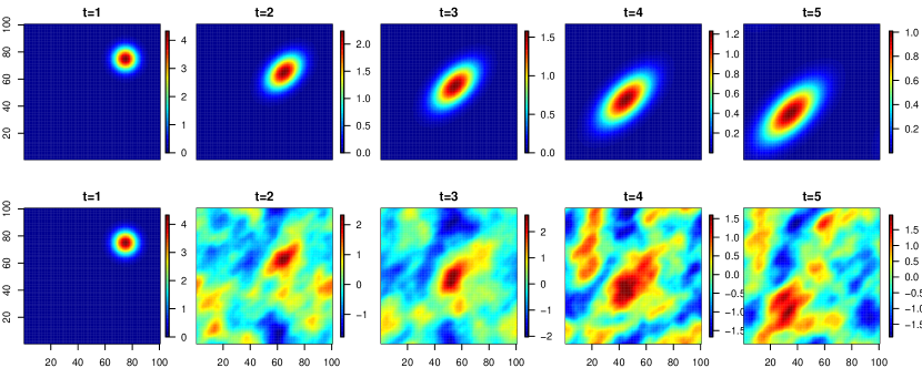
Figure 1: Illustration of the SPDE in (1) and the corresponding PDE. The top row illustrates a solution to the PDE which corresponds to the deterministic part of the SPDE without stochastic term $\epsilon(t,{\boldsymbol{s}})$. The bottom row shows one sample from the distribution specified by the SPDE with a fixed initial condition. The drift vector points from north-east to south-west and the diffusive part exhibits anisotropy in the same direction. The same parameters are used for both the PDE and the SPDE: $\zeta=-\log(0.99),\rho_{1}=0.06,\gamma=3,\psi=\pi/4,\mu_{x}=-0.1,\mu_{y}=-0.1$, and for the stochastic innovations: $\rho_{0}=0.05,\sigma^{2}=0.7^{2}$. The color scales are different in different panels.

Figure 1 illustrates the SPDE in (1) and the corresponding PDE without the stochastic innovation term. The top row shows a solution to the PDE which corresponds the deterministic part of the SPDE that is obtained when there is no stochastic term $\epsilon(t,{\boldsymbol{s}})$. The figure shows how the initial state in the top-left plot gets propagated forward in time. The drift vector points from north-east to south-west and the diffusive part exhibits anisotropy in the same direction. A $100\times 100$ grid is used and the PDE is solved in the spectral domain using the method described below in Section 3. There is a fundamental difference between the deterministic PDE and the probabilistic SPDE. In the first case, a deterministic process is modeled directly. In the second case, the SPDE defines a stochastic process. Since the operator is linear and the input Gaussian, this process is a Gaussian process whose covariance function is implicitly defined by the SPDE. The bottom row of Figure 1 shows one sample from this Gaussian process. The same initial state as in the deterministic example is used, i.e., we use a fixed initial state. Except for the stochastic part, the same parameters are used for both the PDE and the SPDE. For the innovations $\epsilon(t,{\boldsymbol{s}})$, we choose a Gaussian process that is temporally independent and spatially structured according to the Matérn covariance function with smoothness parameter $1$. Again, the drift vector points from north-east to south-west and the diffusive part exhibits anisotropy in the same direction.

Note that the use of this spatio-temporal Gaussian process is not restricted to situations where it is a priori known that phenomena such as transport and diffusion occur. In the one dimensional case, it is common to use the AR(1) process in situations where it is not a priori clear whether the modeled process follows the dynamic of the Ornstein-Uhlenbeck SDE. In two dimensions, the same holds true for the process with the Whittle covariance function, and even more so for the process having an exponential covariance structure. Having this in mind, even though the SPDE in (1) is physically motivated, it can be used as a general spatio-temporal model. As the case may be, the interpretation of the parameters can be more or less straightforward.

2.1 Spectral Density and Covariance Function

As can be shown using the Fourier transform (see, e.g., Whittle (1963)), if the innovation process $\epsilon(t,{\boldsymbol{s}})$ is stationary with spectral density $\widetilde{f}({\boldsymbol{k}})$, the spectrum of the stationary solution $\xi(t,{\boldsymbol{s}})$ of the SPDE (1) is

$$f(\omega,{\boldsymbol{k}})=\widetilde{f}({\boldsymbol{k}})\frac{1}{(2\pi)}\left(\left({\boldsymbol{k}}^{T}{\boldsymbol{\Sigma}}{\boldsymbol{k}}+\zeta\right)^{2}+\left(\omega+{\boldsymbol{\mu}}^{T}{\boldsymbol{k}}\right)^{2}\right)^{-1},$$ (3)

where ${\boldsymbol{k}}$ and $\omega$ are spatial wavenumbers and temporal frequencies. The covariance function $C(t,{\boldsymbol{s}})$ of $\xi(t,{\boldsymbol{s}})$ is then given by

$$\begin{split}C(t,{\boldsymbol{s}})=&\int f(\omega,{\boldsymbol{k}}){\exp\left({\imath\cdot t\omega}\right)}{\exp\left({\imath\cdot{\boldsymbol{s}}^{\prime}{\boldsymbol{k}}}\right)}d{\boldsymbol{k}}d\omega\\ =&\int\widetilde{f}({\boldsymbol{k}})\frac{{\exp\left({-\imath\cdot{\boldsymbol{\mu}}^{T}{\boldsymbol{k}}t-({\boldsymbol{k}}^{T}{\boldsymbol{\Sigma}}{\boldsymbol{k}}+\zeta)|t|}\right)}}{2({\boldsymbol{k}}^{T}{\boldsymbol{\Sigma}}{\boldsymbol{k}}+\zeta)}{\exp\left({\imath\cdot{\boldsymbol{s}}^{\prime}{\boldsymbol{k}}}\right)}d{\boldsymbol{k}},\end{split}$$ (4)

where $\imath$ denotes the imaginary number $\imath^{2}=-1$, and the integration over the temporal frequencies $\omega$ follows from the calculation of the characteristic function of the Cauchy distribution (Abramowitz and Stegun 1964). The spatial integral above has no closed form solution but can be computed approximately by numerical integration.

Since, in general, the spectrum does not factorize into a temporal and a spatial component, we see that $\xi(t,{\boldsymbol{s}})$ has a non-separable covariance function (see Gneiting et al. (2007) for a definition of separability). The model reduces to a separable one, though, when there is no advection and diffusion, i.e., when both ${\boldsymbol{\mu}}$ and ${\boldsymbol{\Sigma}}$ are zero. In this case, the covariance function is given by $C(t,{\boldsymbol{s}})=\frac{1}{2\zeta}{\exp\left({-\zeta|t|}\right)}C({\boldsymbol{s}})$, where $C({\boldsymbol{s}})$ denotes the spatial covariance function of the innovation process.

2.2 Specification of the Innovation Process

It is assumed that the innovation process is white in time and spatially colored. In principle, one can choose any spatial covariance function such that the covariance function in (4) is finite at zero. Note that if $\widetilde{f}({\boldsymbol{k}})$ is integrable, then $f(\omega,{\boldsymbol{k}})$ is also integrable. Similarly as Lindgren et al. (2011), we opt for the most commonly used covariance function in spatial statistics: the Matérn covariance function (see Handcock and Stein (1993), Stein (1999)). Since in many applications the smoothness parameter is not estimable, we further restrict ourselves to the Whittle covariance function. This covariance function is of the form $\sigma^{2}d/\rho_{0}K_{1}\left(d/\rho_{0}\right)$ with $d$ being the Euclidean distance between two points and $K_{1}\left(d/\rho_{0}\right)$ being the modified Bessel function of order $1$. It is called after Whittle (1954) who introduced it and argued convincingly that it “may be regarded as the ’elementary’ correlation in two dimensions, similar to the exponential in one dimension.”. It can be shown that the stationary solution of the SPDE

$$\left(\nabla\cdot\nabla-\frac{1}{\rho_{0}^{2}}\right)\epsilon(t,{\boldsymbol{s}})=\mathcal{W}(t,{\boldsymbol{s}}),$$ (5)

where $\mathcal{W}(t,{\boldsymbol{s}})$ is a zero mean Gaussian white noise field with variance $\sigma^{2}$, has the Whittle covariance function in space. From this, it follows that the spectrum of the process $\epsilon(t,{\boldsymbol{s}})$ is given by

$$\widetilde{f}({\boldsymbol{k}})=\frac{\sigma^{2}}{(2\pi)^{2}}\left({\boldsymbol{k}}^{T}{\boldsymbol{k}}+\frac{1}{\rho_{0}^{2}}\right)^{-2},~{}~{}\rho_{0}>0,~{}\sigma>0.$$ (6)

The parameter $\sigma^{2}$ determines the marginal variance of $\epsilon(t,{\boldsymbol{s}})$, and $\rho_{0}$ is a spatial range parameter.

2.3 Relation to an Integro-Difference Equation

Assuming discrete time steps with lag $\Delta$, Brown et al. (2000) consider the following integro-difference equation (IDE)

$$\xi(t,{\boldsymbol{s}})={\exp\left({-\Delta\zeta}\right)}\int_{\mathbb{R}^{2}}{h({\boldsymbol{s}}-{\boldsymbol{s}}^{\prime})\xi(t-\Delta,{\boldsymbol{s}}^{\prime})d{\boldsymbol{s}}^{\prime}}+\epsilon(t,{\boldsymbol{s}}),~{}~{}{\boldsymbol{s}}\in\mathbb{R}^{2},$$ (7)

with a Gaussian redistribution kernel

$$h({\boldsymbol{s}}-{\boldsymbol{s}}^{\prime})=(2\pi)^{-1}|2\Delta{\boldsymbol{\Sigma}}|^{-1/2}\exp\left(-({\boldsymbol{s}}-{\boldsymbol{s}}^{\prime}-\Delta{\boldsymbol{\mu}})^{T}(2\Delta{\boldsymbol{\Sigma}})^{-1}({\boldsymbol{s}}-{\boldsymbol{s}}^{\prime}-\Delta{\boldsymbol{\mu}})/2\right),$$

$\epsilon(t,{\boldsymbol{s}})$ being temporally independent and spatially dependent. They show that in the limit $\Delta\to 0$, the solution of the IDE and the one of the SPDE in (1) coincide. The IDE is interpreted as follows: the convolution kernel $h({\boldsymbol{s}}-{\boldsymbol{s}}^{\prime})$ determines the weight or the amount of influence that a location ${\boldsymbol{s}}^{\prime}$ at previous time $t-\Delta$ has on the point ${\boldsymbol{s}}$ at current time $t$. This IDE representation provides an alternative way of interpreting the SPDE model and its parameters. Storvik et al. (2002) show under which conditions a dynamic model determined by an IDE as in (7) can be represented using a parametric joint space-time covariance function, and vice versa. Based on the IDE in (7), Sigrist et al. (2012) construct a spatio-temporal model for irregularly spaced data and apply it to obtain short term predictions of precipitation. Wikle (2002) and Xu et al. (2005) also model spatio-temporal rainfall based on IDEs.

3   Solution in the Spectral Space

Solutions $\xi(t,{\boldsymbol{s}})$ of the SPDE (1) are defined in continuous space and time. In practice, one needs to discretize both space and time. The resulting vector of $NT$ space-time points is in general of large dimension. This makes statistical inference, be it frequentist or Bayesian, computationally difficult to impossible. However, as we show in the following, solving the SPDE in the spectral space alleviates the computational burden considerably and allows for dimension reduction, if desired.

Heuristically speaking, spectral methods (Gottlieb and Orszag 1977; Cressie and Wikle 2011, Chapter 7) approximate the solution $\xi(t,{\boldsymbol{s}})$ by a linear combination of deterministic spatial functions $\phi_{j}({\boldsymbol{s}})$ with random coefficients $\alpha_{j}(t)$ that evolve dynamically over time:

$$\begin{split}\xi^{K}(t,{\boldsymbol{s}})&=\sum_{j=1}^{K}{\alpha_{j}(t)\phi_{j}({\boldsymbol{s}})}={\boldsymbol{\phi}}({\boldsymbol{s}})^{T}{\boldsymbol{\alpha}}(t),\end{split}$$ (8)

where ${\boldsymbol{\phi}}({\boldsymbol{s}})=(\phi_{1}({\boldsymbol{s}}),\dots,\phi_{K}({\boldsymbol{s}}))^{T}$ and ${\boldsymbol{\alpha}}(t)=(\alpha_{1}(t),\dots,\alpha_{K}(t))^{T}$. To be more specific, we use Fourier functions

$$\phi_{j}({\boldsymbol{s}})=\exp{(\imath\cdot{\boldsymbol{k}}_{j}^{T}{\boldsymbol{s}})},$$ (9)

where ${\boldsymbol{k}}_{j}=(k_{j}^{x},k_{j}^{y})^{T}$ is a spatial wavenumber.

The advantages of using Fourier functions for solving linear, deterministic PDEs are well known, see, e.g., Pedlosky (1987). First, differentiation in the physical space corresponds to multiplication in the spectral space. In other words, Fourier functions are eigenfunctions of the spatial differential operator. Instead of approximating the differential operator in the physical space and then worrying about approximation errors, one just has to multiply in the spectral space, and there is no approximation error of the operator when all the basis functions are retained. In addition, one can use the FFT for efficiently transforming from the physical to the spectral space, and vice versa.

Proposition 1 shows that Fourier functions are also useful for the stochastic PDE (1): if the initial condition and the innovation process are in the space spanned by a finite number of Fourier functions, then the solution of the SPDE (1) remains in this space for all times and can be given in explicit form.

Proposition 1.

Assume that the initial state and the innovation terms are of the form

$$\xi^{K}(0,{\boldsymbol{s}})={\boldsymbol{\phi}}({\boldsymbol{s}})^{T}{\boldsymbol{\alpha}}(0),\quad\epsilon^{K}(t,{\boldsymbol{s}})={\boldsymbol{\phi}}({\boldsymbol{s}})^{T}\widetilde{{\boldsymbol{\epsilon}}}(t)$$ (10)

where ${\boldsymbol{\phi}}({\boldsymbol{s}})=(\phi_{1}({\boldsymbol{s}}),\dots,\phi_{K}({\boldsymbol{s}}))^{T}$, $\phi_{j}({\boldsymbol{s}})$ is given in (9), ${\boldsymbol{\alpha}}(0)\sim N\left({\boldsymbol{0}},\textnormal{diag}\left(\widetilde{f}_{0}({\boldsymbol{k}}_{j})\right)\right)$, $\widetilde{f}_{0}(\cdot)$ being a spectral density, and $\widetilde{{\boldsymbol{\epsilon}}}(t)$ is a $K$-dimensional Gaussian white noise independent of ${\boldsymbol{\alpha}}(0)$ with

$$\mathrm{Cov}(\widetilde{{\boldsymbol{\epsilon}}}(t),\widetilde{{\boldsymbol{\epsilon}}}(t^{\prime}))=\delta_{t,t^{\prime}}\textnormal{diag}\left(\widetilde{f}({\boldsymbol{k}}_{j})\right),$$ (11)

where $\widetilde{f}(\cdot)$ is a spectral density and $\delta_{t,t^{\prime}}$ the Kronecker delta function equaling $1$ if $t=t^{\prime}$ and zero otherwise. Then the process $\xi^{K}(t,{\boldsymbol{s}})={\boldsymbol{\phi}}({\boldsymbol{s}})^{T}{\boldsymbol{\alpha}}(t)$, where the components $\alpha_{j}(t)$ are given by

$$\alpha_{j}(t)={\exp\left({h_{j}t}\right)}\alpha_{j}(0)+\int_{0}^{t}{\exp\left({h_{j}(t-u)}\right)}\widetilde{\epsilon}_{j}(u)du$$ (12)

with $h_{j}=-\imath\cdot{\boldsymbol{\mu}}^{T}{\boldsymbol{k}}_{j}-{\boldsymbol{k}}_{j}^{T}{\boldsymbol{\Sigma}}{\boldsymbol{k}}_{j}-\zeta$, is a solution of the SPDE in (1). For $t\rightarrow\infty$, the influence of the initial condition $\exp(h_{j}t)\alpha_{j}(0)$ converges to zero and the process $\xi^{K}(t,{\boldsymbol{s}})$ converges to a time stationary Gaussian process with mean zero and

$$\mathrm{Cov}(\xi^{K}(t+\Delta t,{\boldsymbol{s}}),\xi^{K}(t,{\boldsymbol{s}}^{\prime}))={\boldsymbol{\phi}}({\boldsymbol{s}})^{T}\textnormal{diag}\left(\frac{-{\exp\left({h_{j}\Delta t}\right)}\widetilde{f}({\boldsymbol{k}}_{j})}{h_{j}+h_{j}^{\ast}}\right){\boldsymbol{\phi}}({\boldsymbol{s}}^{\prime})^{\ast},$$

where $.^{\ast}$ stands for complex conjugation.

This result shows that the solution of the SPDE is exact over time, given the frequencies included. In contrast to finite differences, one does not accumulate errors over time. This is related to the fact that there is no need for numerical stability conditions. For statistical applications, where the parameters are not known a priori, this is particularly useful. The approximation error of $\xi^{K}(t,{\boldsymbol{s}})$ to the space time stationary solution of the SPDE in (1) only depends on the number of spectral terms and not on the temporal discretization, see also Proposition 2 below. Since Fourier terms are global functions, stationarity in space, but not in time, is a necessary assumption.

Proof.

By (12), we have

$$\begin{split}\frac{\partial}{\partial t}\xi^{K}(t,{\boldsymbol{s}})&=\sum_{j=1}^{K}{\dot{\alpha}_{j}(t)\phi_{j}({\boldsymbol{s}})}=\sum_{j=1}^{K}{(h_{j}\alpha_{j}(t)+\widetilde{\epsilon}_{j}(t))\phi_{j}({\boldsymbol{s}})}.\end{split}$$

On the other hand, since the functions $\phi_{j}({\boldsymbol{s}})=\exp{(\imath\cdot{\boldsymbol{k}}_{j}^{T}{\boldsymbol{s}})}$ are Fourier terms, differentiation in the physical space corresponds to multiplication in the spectral space:

$${\boldsymbol{\mu}}^{T}\nabla\phi_{j}({\boldsymbol{s}})=i{\boldsymbol{\mu}}^{T}{\boldsymbol{k}}_{j}\phi_{j}({\boldsymbol{s}})$$ (13)

and

$$\nabla\cdot{\boldsymbol{\Sigma}}\nabla\phi_{j}({\boldsymbol{s}})=-{\boldsymbol{k}}_{j}^{T}{\boldsymbol{\Sigma}}{\boldsymbol{k}}_{j}\phi_{j}({\boldsymbol{s}}).$$ (14)

Therefore, by the definition of $h_{j}$,

$$\left(-{\boldsymbol{\mu}}^{T}\nabla+\nabla\cdot{\boldsymbol{\Sigma}}\nabla-\zeta\right)\sum_{j=1}^{K}\alpha_{j}(t)\phi_{j}({\boldsymbol{s}})=\sum_{j=1}^{K}h_{j}\alpha_{j}(t)\phi_{j}({\boldsymbol{s}}).$$

Together, we have

$$\frac{\partial}{\partial t}\xi^{K}(t,{\boldsymbol{s}})=\left(-{\boldsymbol{\mu}}^{T}\nabla+\nabla\cdot{\boldsymbol{\Sigma}}\nabla-\zeta\right)\xi^{K}(t,{\boldsymbol{s}})+\epsilon^{K}(t,{\boldsymbol{s}})$$

which proves the first part of the proposition. Since the real part of $h_{j}$ is negative, $\exp(h_{j}t)\rightarrow 0$ for $t\rightarrow\infty$. Moreover,

$$\begin{split}\lim\limits_{t\rightarrow\infty}\mathrm{Cov}(\alpha_{j}(t+\Delta t),\alpha_{j^{\prime}}(t))&=\lim\limits_{t\rightarrow\infty}{\exp\left({h_{j}\Delta t}\right)}\delta_{j,j^{\prime}}\widetilde{f}({\boldsymbol{k}}_{j})\int_{0}^{t}{\exp\left({-(h_{j}+h_{j^{\prime}}^{\ast})(t-u)}\right)}du\\ &=-\frac{{\exp\left({h_{j}\Delta t}\right)}}{h_{j}+h_{j}^{\ast}}\delta_{j,j^{\prime}}\widetilde{f}({\boldsymbol{k}}_{j}),\end{split}$$ (15)

and thus the last statement follows. ∎

We assume that the forcing term $\epsilon(t,.)$, the initial state $\xi(0,.)$, and consequently also the solution $\xi(t,.)$, are stationary in space. Recall the Cramér representation for a stationary field $\epsilon(t,.)$

$$\epsilon(t,{\boldsymbol{s}})=\int\exp{(\imath\cdot{\boldsymbol{k}}^{T}{\boldsymbol{s}})}d\widetilde{\epsilon}_{t}({\boldsymbol{k}})$$

where $\widetilde{\epsilon}_{t}$ has orthogonal increments $\mathrm{Cov}(d\widetilde{\epsilon}_{t}({\boldsymbol{k}}),d\widetilde{\epsilon}_{t^{\prime}}({\boldsymbol{l}}))=\delta_{t,t^{\prime}}\delta_{{\boldsymbol{k}},{\boldsymbol{l}}}\widetilde{f}({\boldsymbol{k}})$ and $\widetilde{f}(\cdot)$ is the spectral density of $\epsilon(t,.)$ (see, e.g., Cramér and Leadbetter (1967)). This implies that we can approximate any stationary field, in particular also the one with a Whittle covariance function, by a finite linear combination of complex exponentials, and the covariance of $\widetilde{{\boldsymbol{\epsilon}}}(t)$ is a diagonal matrix as required in the proposition. Its entries are specified in (6). Concerning the initial state, one can use the stationary distribution of $\xi(t,.)$. An alternative choice is to use the same spatial distribution as for the innovations: $\widetilde{f}_{0}(\cdot)=\widetilde{f}(\cdot)$.

3.1 Approximation bound

By passing to the limit $K\rightarrow\infty$ such that both the wavenumbers ${\boldsymbol{k}}_{j}$ cover the entire domain $\mathbb{R}^{2}$ and the distance between neighboring wavenumbers goes to zero, we obtain from (8) the stationary (in space and time) solution with spectral density as in (3). In practice, if one uses the discrete Fourier transform (DFT), or its fast variant, the FFT, the wavenumbers are regularly spaced and the distance between them is fixed for all $K$ (see below). This implies that the covariance function of an approximate solution is periodic which is equivalent to assuming a rectangular domain being wrapped around a torus. Since in most applications, the domain is fixed anyway, this is a reasonable assumption.

Based on the above considerations, we assume, in the following, that ${\boldsymbol{s}}\in[0,1]^{2}$ with periodic boundary condition, i.e., that $[0,1]^{2}$ is wrapped on a torus. In practice, to avoid spurious periodicity, we can apply what is called “padding”. This means that we take ${\boldsymbol{s}}\in[0,0.5]^{2}$ and then embed it in $[0,1]^{2}$. As in the discrete Fourier transform, if we choose ${\boldsymbol{s}}\in[0,1]^{2}$, it follows that the spatial wavenumbers ${\boldsymbol{k}}_{j}$ lie on the $n\times n$ grid given by $D_{n}=\{2\pi\cdot(i,j):-(n/2+1)\leq i,j\leq n/2\}=\{-2\pi(n/2+1),\dots,2\pi n/2\}^{2}$ with $n^{2}=N=K$, $n$ being an even natural number. We then have the following convergence result.

Proposition 2.

When $N\rightarrow\infty$, the approximation $\xi^{N}(t,{\boldsymbol{s}})$ converges in law to the solution $\xi(t,{\boldsymbol{s}})$ of the SPDE (1) with ${\boldsymbol{s}}\in[0,1]^{2}$ wrapped on a torus, and we have the bound

$$|C(t,{\boldsymbol{s}})-C^{N}(t,{\boldsymbol{s}})|\leq\sigma^{2}_{\xi}-\sigma^{2}_{\xi^{N}},$$ (16)

where $C(t,{\boldsymbol{s}})$ and $C^{N}(t,{\boldsymbol{s}})$ denote the covariance functions of $\xi(t,{\boldsymbol{s}})$ and $\xi^{N}(t,{\boldsymbol{s}})$, respectively, and where $\sigma^{2}_{\xi}=C(0,{\boldsymbol{0}})$ and $\sigma^{2}_{\xi^{N}}=C^{N}(0,{\boldsymbol{0}})$ denote the marginal variances of these two processes.

Proof.

Similarly as in (4) and due to ${\boldsymbol{k}}\in 2\pi\cdot\mathbb{Z}^{2}$, it follows that the covariance function of $\xi(t,{\boldsymbol{s}})$ is given by

$$\begin{split}C(t,{\boldsymbol{s}})=&\sum_{{\boldsymbol{k}}\in 2\pi\cdot\mathbb{Z}^{2}}\int f(\omega,{\boldsymbol{k}}){\exp\left({\imath\cdot t\omega}\right)}d\omega\exp(\imath\cdot{\boldsymbol{s}}^{\prime}{\boldsymbol{k}})\\ =&\sum_{{\boldsymbol{k}}\in 2\pi\cdot\mathbb{Z}^{2}}\widetilde{f}({\boldsymbol{k}})\frac{-{\exp\left({h_{{\boldsymbol{k}}}t}\right)}}{h_{{\boldsymbol{k}}}+h_{{\boldsymbol{k}}}^{*}}\exp(\imath\cdot{\boldsymbol{s}}^{\prime}{\boldsymbol{k}}),\end{split}$$ (17)

where $h_{{\boldsymbol{k}}}=-\imath\cdot{\boldsymbol{\mu}}^{T}{\boldsymbol{k}}-{\boldsymbol{k}}^{T}{\boldsymbol{\Sigma}}{\boldsymbol{k}}-\zeta$. From Proposition 1 we know that the approximate solution $\xi^{N}(t,{\boldsymbol{s}})$ has the covariance function

$$C^{N}(t,{\boldsymbol{s}})=\sum_{{\boldsymbol{k}}\in D_{n}}\widetilde{f}({\boldsymbol{k}})\frac{-{\exp\left({h_{{\boldsymbol{k}}}t}\right)}}{h_{{\boldsymbol{k}}}+h_{{\boldsymbol{k}}}^{*}}\exp(\imath\cdot{\boldsymbol{s}}^{\prime}{\boldsymbol{k}}).$$ (18)

It follows that

$$\begin{split}|C(t,{\boldsymbol{s}})-C^{N}(t,{\boldsymbol{s}})|=&\left|\sum_{{\boldsymbol{k}}\in 2\pi\cdot\mathbb{Z}^{2}}\widetilde{f}({\boldsymbol{k}})\frac{-{\exp\left({h_{{\boldsymbol{k}}}t}\right)}}{h_{{\boldsymbol{k}}}+h_{{\boldsymbol{k}}}^{*}}(1-\mathbbmss{1}_{\{{\boldsymbol{k}}\in D_{n}\}})\exp(\imath\cdot{\boldsymbol{s}}^{\prime}{\boldsymbol{k}})\right|\\ \leq&\sum_{{\boldsymbol{k}}\in 2\pi\cdot\mathbb{Z}^{2}}\widetilde{f}({\boldsymbol{k}})\frac{-1}{h_{{\boldsymbol{k}}}+h_{{\boldsymbol{k}}}^{*}}(1-\mathbbmss{1}_{\{{\boldsymbol{k}}\in D_{n}\}})\\ =&\sigma^{2}_{\xi}-\sigma^{2}_{\xi^{N}}.\end{split}$$ (19)

∎

Not surprisingly, this result tells us that the rate of convergence essentially depends on the smoothness properties of the process $\xi(t,{\boldsymbol{s}})$, i.e., on how fast the spectrum decays. The smoother $\xi(t,{\boldsymbol{s}})$, that is, the more variation is explained by low frequencies, the faster is the convergence of the approximation.

Note that there is a conceptual difference between the stationary solution of the SPDE (1) with ${\boldsymbol{s}}\in\mathbb{R}^{2}$ and the periodic one with ${\boldsymbol{s}}\in[0,1]^{2}$ wrapped on a torus. For the sake of notational simplicity, we have denoted both of them by $\xi(t,{\boldsymbol{s}})$. The finite dimensional solution $\xi^{N}(t,{\boldsymbol{s}})$ is an approximation to both of the above infinite dimensional solutions. The above convergence result, though, only holds true for the solution on the torus.

3.2 Real Fourier Functions and Discretization in Time and Space

To apply the model to real data, we have to discretize it. In the following, we consider the process $\xi(t,{\boldsymbol{s}})$ on a regular grid of $n\times n=N$ spatial locations ${\boldsymbol{s}}_{1},\dots,{\boldsymbol{s}}_{N}$ in $[0,1]^{2}$ and at equidistant time points $t_{1},\dots,t_{T}$ with $t_{i}-t_{i-1}=\Delta$. Note that these two assumptions can be easily relaxed, i.e., one can have irregular spatial observation locations and non-equidistant time points. The former can be achieved by adopting a data augmentation approach (see, for instance, Sigrist et al. (2012)) or by using an incidence matrix (see Section 4.2). The latter can be done by taking a time varying $\Delta$.

For the sake of illustration, we have stated the results in the previous section using complex Fourier functions. However, when discretizing the model, one obtains a linear Gaussian state space model with a propagator matrix ${\boldsymbol{G}}$ that contains complex numbers, due to (13). To avoid this, we replace the complex terms $\exp{(\imath\cdot{\boldsymbol{k}}_{j}^{T}{\boldsymbol{s}})}$ with real $\cos({\boldsymbol{k}}_{j}^{T}{\boldsymbol{s}})$ and $\sin({\boldsymbol{k}}_{j}^{T}{\boldsymbol{s}})$ functions. In other words, we use the real instead of the complex Fourier transform. The above results then still hold true, since for real valued data, the real Fourier transform is equivalent to the complex one. For notational simplicity, we will drop the superscript “^K” from $\xi^{K}(t,{\boldsymbol{s}})$. The distinction between the approximation and the true solution is clear from the context.

Proposition 3.

On the above specified discretized spatial and temporal domain and using the real Fourier transform, with initial state ${\boldsymbol{\alpha}}(t_{0})\sim N(0,\widetilde{{\boldsymbol{Q}}}_{0})$, $\widetilde{{\boldsymbol{Q}}}_{0}$ diagonal, a stationary solution of the SPDE (1) is of the form

$${\boldsymbol{\xi}}(t_{i+1}) ={\boldsymbol{\Phi}}{\boldsymbol{\alpha}}(t_{i+1}),$$ (20)

$${\boldsymbol{\alpha}}(t_{i+1}) ={\boldsymbol{G}}{\boldsymbol{\alpha}}(t_{i})+\widetilde{{\boldsymbol{\epsilon}}}(t_{i+1}),~{}~{}\widetilde{{\boldsymbol{\epsilon}}}(t_{i+1})\sim N(0,\widetilde{{\boldsymbol{Q}}}),$$ (21)

with stacked vectors ${\boldsymbol{\xi}}(t_{i})=(\xi(t_{i},{\boldsymbol{s}}_{1}),\dots,\xi(t_{i},{\boldsymbol{s}}_{N}))^{T}$ and cosine and sine coefficients ${\boldsymbol{\alpha}}(t_{i})=\left(\alpha_{1}^{(c)}(t_{i}),\dots,\alpha_{4}^{(c)}(t_{i}),\alpha_{5}^{(c)}(t_{i}),\alpha_{5}^{(s)}(t_{i}),\dots,\alpha_{K/2+2}^{(c)}(t_{i}),\alpha_{K/2+2}^{(s)}(t_{i})\right)^{T},$ where ${\boldsymbol{\Phi}}$ applies the discrete, real Fourier transformation, ${\boldsymbol{G}}$ is a block diagonal matrix with $2\times 2$ blocks, and $\widetilde{{\boldsymbol{Q}}}$ is a diagonal matrix. The above matrices are defined as follows.

• ${\boldsymbol{\Phi}}=\left[{\boldsymbol{\phi}}({\boldsymbol{s}}_{1}),\dots,{\boldsymbol{\phi}}({\boldsymbol{s}}_{N})\right]^{T},$
  ${\boldsymbol{\phi}}({\boldsymbol{s}}_{l})=\left(\phi_{1}^{(c)}({\boldsymbol{s}}_{l}),\dots,\phi_{4}^{(c)}({\boldsymbol{s}}_{l}),\phi_{5}^{(c)}({\boldsymbol{s}}_{l}),\phi_{5}^{(s)}({\boldsymbol{s}}_{l}),\dots,\phi_{K/2+2}^{(c)}({\boldsymbol{s}}_{l}),\phi_{K/2+2}^{(s)}({\boldsymbol{s}}_{l})\right)^{T},$
  $\phi^{(c)}_{j}({\boldsymbol{s}}_{l})=\cos({\boldsymbol{k}}_{j}^{T}{\boldsymbol{s}}_{l}),~{}~{}\phi^{(s)}_{j}({\boldsymbol{s}}_{l})=\sin({\boldsymbol{k}}_{j}^{T}{\boldsymbol{s}}_{l})$, $\l=1,\dots,n^{2}$

• $[{\boldsymbol{G}}]_{1:4,1:4}=\textnormal{diag}\left({\exp\left({-\Delta({\boldsymbol{k}}_{j}^{T}{\boldsymbol{\Sigma}}{\boldsymbol{k}}_{j}+\zeta)}\right)}\right),$

  $[{\boldsymbol{G}}]_{5:K,5:K}=\textnormal{diag}\left({\exp\left({-\Delta({\boldsymbol{k}}_{j}^{T}{\boldsymbol{\Sigma}}{\boldsymbol{k}}_{j}+\zeta)}\right)}\left(\cos(\Delta{\boldsymbol{\mu}}^{T}{\boldsymbol{k}}_{j}){\boldsymbol{1}}_{2}-\sin(\Delta{\boldsymbol{\mu}}^{T}{\boldsymbol{k}}_{j}){\boldsymbol{J}}_{2}\right)\right),$ where

  $${\boldsymbol{1}}_{2}=\left(\begin{matrix}1&0\\ 0&1\end{matrix}\right),~{}~{}{\boldsymbol{J}}_{2}=\left(\begin{matrix}0&1\\ -1&0\end{matrix}\right),$$ (22)

• $\widetilde{{\boldsymbol{Q}}}=\text{{diag}}\left(\widetilde{f}({\boldsymbol{k}}_{j})\frac{1-{\exp\left({-2\Delta({\boldsymbol{k}}_{j}^{T}{\boldsymbol{\Sigma}}{\boldsymbol{k}}_{j}+\zeta)}\right)}}{2({\boldsymbol{k}}_{j}^{T}{\boldsymbol{\Sigma}}{\boldsymbol{k}}_{j}+\zeta)}\right),$

• $\widetilde{{\boldsymbol{Q}}}_{0}=({\boldsymbol{1}}_{N}-{\boldsymbol{G}}{\boldsymbol{G}}^{T})^{-1}\widetilde{{\boldsymbol{Q}}}$.

In summary, at each time point $t$ and spatial point ${\boldsymbol{s}}_{l}$, $l=1,\dots,n^{2}$, the solution $\xi(t,{\boldsymbol{s}}_{l})$ is the discrete real Fourier transform of the random coefficients ${\boldsymbol{\alpha}}(t)$

$$\begin{split}\xi(t,{\boldsymbol{s}}_{l})&=\sum_{j=1}^{4}\alpha^{(c)}_{j}(t)\phi^{(c)}_{j}({\boldsymbol{s}}_{l})+\sum_{j=5}^{K/2+2}{\left(\alpha^{(c)}_{j}(t)\phi^{(c)}_{j}({\boldsymbol{s}}_{l})+\alpha^{(s)}_{j}(t)\phi^{(s)}_{j}({\boldsymbol{s}}_{l})\right)}\\ &={\boldsymbol{\phi}}({\boldsymbol{s}}_{l})^{T}{\boldsymbol{\alpha}}(t),\end{split}$$ (23)

and the Fourier coefficients ${\boldsymbol{\alpha}}(t)$ evolve dynamically over time according to the vector autoregression in (21). The first four terms are cosine terms and, afterward, there are cosine - sine pairs. This is a peculiarity of the real Fourier transform. It is due to the fact that for four wavenumbers ${\boldsymbol{k}}_{j}$, the sine terms equal zero on the grid, i.e., $\sin({\boldsymbol{k}}_{j}^{T}{\boldsymbol{s}}_{l})=0$, for all $l=1,\dots,n^{2}$ and ${\boldsymbol{k}}_{j}\in\{(0,0)^{T},(0,n\pi)^{T},(n\pi,0)^{T},(n\pi,n\pi)^{T}\}$ (see Figure 3). The above equations (20) and (21) form a linear Gaussian state space model with parametric propagator matrix ${\boldsymbol{G}}$ and innovation covariance matrix $\widetilde{{\boldsymbol{Q}}}$, the parametrization being determined by the corresponding SPDE.

The model in (20) and (21) is similar to the one discussed in Cressie and Wikle (2011, Chapter 7), but the derivation as an exact solution to the stochastic PDE (1) rather than a deterministic PDE is different.

Proof.

Similarly as in Proposition 1, we first derive the continuous time solution. Using

$${\boldsymbol{\mu}}^{T}\nabla\phi^{(c)}_{j}({\boldsymbol{s}}_{l})=-{\boldsymbol{\mu}}^{T}{\boldsymbol{k}}_{j}\phi^{(s)}_{j}({\boldsymbol{s}}_{l}),~{}~{}{\boldsymbol{\mu}}^{T}\nabla\phi^{(s)}_{j}({\boldsymbol{s}}_{l})={\boldsymbol{\mu}}^{T}{\boldsymbol{k}}_{j}\phi^{(c)}_{j}({\boldsymbol{s}}_{l}),$$

$$\nabla\cdot{\boldsymbol{\Sigma}}\nabla\phi^{(c)}_{j}({\boldsymbol{s}}_{l})=-{\boldsymbol{k}}_{j}^{T}{\boldsymbol{\Sigma}}{\boldsymbol{k}}_{j}\phi^{(c)}_{j}({\boldsymbol{s}}_{l}),~{}~{}\nabla\cdot{\boldsymbol{\Sigma}}\nabla\phi^{(s)}_{j}({\boldsymbol{s}}_{l})=-{\boldsymbol{k}}_{j}^{T}{\boldsymbol{\Sigma}}{\boldsymbol{k}}_{j}\phi^{(s)}_{j}({\boldsymbol{s}}_{l}),$$

and the same arguments as in the proof of Proposition 1, it follows that the continuous time solution is of the form (23). For each pair of cosine - sine coefficients ${\boldsymbol{\alpha}}_{j}(t)=(\alpha^{(c)}_{j}(t),\alpha^{(s)}_{j}(t))^{T}$ we have

$${\boldsymbol{\alpha}}_{j}(t)=e^{{\boldsymbol{H}}_{j}t}{\boldsymbol{\alpha}}_{j}(0)+\int_{0}^{t}e^{{\boldsymbol{H}}_{j}(t-u)}\widetilde{{\boldsymbol{\epsilon}}}_{j}(u)du,$$ (24)

where

$${\boldsymbol{H}}_{j}=\left(\begin{matrix}-{\boldsymbol{k}}_{j}^{T}{\boldsymbol{\Sigma}}{\boldsymbol{k}}_{j}-\zeta&-{\boldsymbol{\mu}}^{T}{\boldsymbol{k}}_{j}\\ {\boldsymbol{\mu}}^{T}{\boldsymbol{k}}_{j}&-{\boldsymbol{k}}_{j}^{T}{\boldsymbol{\Sigma}}{\boldsymbol{k}}_{j}-\zeta\end{matrix}\right).$$

Now ${\boldsymbol{H}}_{j}$ can be written as

$${\boldsymbol{H}}_{j}=(-{\boldsymbol{k}}_{j}^{T}{\boldsymbol{\Sigma}}{\boldsymbol{k}}_{j}-\zeta){\boldsymbol{1}}_{2}-{\boldsymbol{\mu}}^{T}{\boldsymbol{k}}_{j}{\boldsymbol{J}_{2}},$$

where

$${\boldsymbol{1}}_{2}=\left(\begin{matrix}1&0\\ 0&1\end{matrix}\right),~{}~{}{\boldsymbol{J}}_{2}=\left(\begin{matrix}0&1\\ -1&0\end{matrix}\right).$$

Since ${\boldsymbol{1}}_{2}$ and ${\boldsymbol{J}}_{2}$ commute, we have

$$\begin{split}e^{{\boldsymbol{H}}_{j}t}=&{\exp\left({-t({\boldsymbol{k}}_{j}^{T}{\boldsymbol{\Sigma}}{\boldsymbol{k}}_{j}+\zeta){\boldsymbol{1}}_{2}}\right)}{\exp\left({-t{\boldsymbol{\mu}}^{T}{\boldsymbol{k}}_{j}{\boldsymbol{J}}_{2}}\right)}\\ =&{\exp\left({-t({\boldsymbol{k}}_{j}^{T}{\boldsymbol{\Sigma}}{\boldsymbol{k}}_{j}+\zeta)}\right)}\left(\cos(t{\boldsymbol{\mu}}^{T}{\boldsymbol{k}}_{j}){\boldsymbol{1}}_{2}-\sin(t{\boldsymbol{\mu}}^{T}{\boldsymbol{k}}_{j}){\boldsymbol{J}}_{2}\right).\end{split}$$ (25)

For the calculation of the exponential function of the matrix ${\boldsymbol{J}}_{2}$, see, e.g., Bronson and Costa (2007, Chapter 4).

Analogously, one derives for the first four cosine terms

$$\alpha_{j}^{c}(t)=e^{-\left({\boldsymbol{k}}_{j}^{T}{\boldsymbol{\Sigma}}{\boldsymbol{k}}_{j}+\zeta\right)t}\alpha_{j}^{c}(0)+\int_{0}^{t}e^{-\left({\boldsymbol{k}}_{j}^{T}{\boldsymbol{\Sigma}}{\boldsymbol{k}}_{j}+\zeta\right)(t-u)}\widetilde{\epsilon}_{j}(u)du,~{}~{}j=1,\dots 4.$$ (26)

The above expression (25) and (26) give the propagator matrix ${\boldsymbol{G}}$.

For the discrete time solution, in addition to the propagation

$${\boldsymbol{\alpha}}_{j}(t+\Delta)=e^{{\boldsymbol{H}}_{j}\Delta}{\boldsymbol{\alpha}}_{j}(t),$$

we need to calculate the covariance of the integrated stochastic innovation term

$$\int_{t}^{t+\Delta}e^{{\boldsymbol{H}}_{j}(t+\Delta-u)}\widetilde{{\boldsymbol{\epsilon}}}_{j}(u)du.$$

This is calculated as

$$\begin{split}\int_{t}^{t+\Delta}e^{{\boldsymbol{H}}_{j}(t+\Delta-u)}\widetilde{f}({\boldsymbol{k}}_{j})e^{{\boldsymbol{H}}^{\prime}_{j}(t+\Delta-u)}du&=\int_{0}^{\Delta}e^{{\boldsymbol{H}}_{j}(\Delta-u)}\widetilde{f}({\boldsymbol{k}}_{j})e^{{\boldsymbol{H}}^{\prime}_{j}(\Delta-u)}du\\ &=\int_{0}^{\Delta}\widetilde{f}({\boldsymbol{k}}_{j}){\exp\left({-2({\boldsymbol{k}}_{j}^{T}{\boldsymbol{\Sigma}}{\boldsymbol{k}}_{j}+\zeta)(\Delta-u)}\right)}{\boldsymbol{1}}_{2}du\\ &=\widetilde{f}({\boldsymbol{k}}_{j})\frac{1-{\exp\left({-2({\boldsymbol{k}}_{j}^{T}{\boldsymbol{\Sigma}}{\boldsymbol{k}}_{j}+\zeta)\Delta}\right)}}{2({\boldsymbol{k}}_{j}^{T}{\boldsymbol{\Sigma}}{\boldsymbol{k}}_{j}+\zeta)}{\boldsymbol{1}}_{2}.\end{split}$$

For the first four cosine terms, calculations are done analogously. The covariance matrix $\widetilde{{\boldsymbol{Q}}}_{0}$ of the initial state ${\boldsymbol{\alpha}}(t_{0})$ is assumed to be the covariance matrix of the stationary distribution of ${\boldsymbol{\alpha}}(t_{i})$. Note that $\widetilde{{\boldsymbol{Q}}}_{0}$ is diagonal since ${\boldsymbol{G}}{\boldsymbol{G}}^{T}$ is diagonal, see the proof of Algorithm 1 in Section 4.1. This then gives the result in (20) and (21). ∎

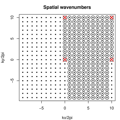
Figure 2: Illustration of spatial wavenumbers for the two-dimensional discrete real Fourier transform with $n^{2}=400$ grid points.

The discrete complex Fourier transform uses $n^{2}$ different wavenumbers ${\boldsymbol{k}}_{j}$ each having a corresponding Fourier term $\exp(\imath\cdot{\boldsymbol{k}}_{j}^{T}{\boldsymbol{s}})$. The real Fourier transform, on the other hand, uses $n^{2}/2+2$ different wavenumbers, where four of them have only a cosine term and the others each have sine and cosine terms. This follows from the fact that, for real data, certain coefficients of the complex transform are the complex transpose of other coefficients. For technical details on the real Fourier transform, we refer to Dudgeon and Mersereau (1984), Borgman et al. (1984), Royle and Wikle (2005), and Paciorek (2007). Figure 2 illustrates an example of the spatial wavenumbers, with $n^{2}=20\times 20=400$ grid points. The dots with a circle represent the wavenumbers actually used in the real Fourier transform, and the red crosses mark the wavenumbers having only a cosine term. Note that in (23) we choose to order the spatial wavenumbers such that the first four spatial wavenumbers correspond to the cosine-only terms.

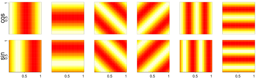
Figure 3: Illustration of two dimensional Fourier basis functions used in the discrete real Fourier transform with $n^{2}=400$. On the x- and y-axis are the coordinates of ${\boldsymbol{s}}$.

To get an idea of what the basis functions $\cos{({\boldsymbol{k}}_{j}^{T}{\boldsymbol{s}})}$ and $\sin{({\boldsymbol{k}}_{j}^{T}{\boldsymbol{s}})}$ look like, we plot in Figure 3 twelve low-frequency basis functions corresponding to the six spatial frequencies closest to the origin ${\boldsymbol{0}}$.

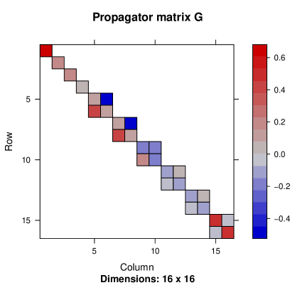
Figure 4: Illustration of propagator matrix ${\boldsymbol{G}}$. 16 real Fourier functions are used ($n=4$).

Further, in Figure 4, there is an example of a propagator matrix ${\boldsymbol{G}}$ when $n=4$, i.e., when sixteen ($4^{2}$) spatial basis functions are used. The upper left $4\times 4$ diagonal matrix corresponds to the cosine-only frequencies. The $2\times 2$ blocks following correspond to wavenumbers with cosine - sine pairs.

Concerning notation in this paper, $K$ refers to the number of Fourier terms, i.e., this is the dimension of the spectral process ${\boldsymbol{\alpha}}(t)$ at each time $t$. Furthermore, $N$ denotes the number of points at which the process ${\boldsymbol{\xi}}(t)$ is modeled, and $n$ is the number of points on each axis of the quadratic grid used. Often, we have $n^{2}=N=K$. However, if one uses a reduced dimensional Fourier basis, $K$ is smaller than $N$, see Section 4.2.

3.3 Remarks on Finite Differences

Another approach to solve PDEs or SPDEs such as the one in (1) consists of using a discretization such as finite differences. Stroud et al. (2010) use finite differences to solve an advection-diffusion PDE. Other examples are Wikle (2003), Xu and Wikle (2007), Duan et al. (2009), Malmberg et al. (2008), and Zheng and Aukema (2010). The finite difference approximation, however, has several disadvantages. First, each spatial discretization effectively implies an interaction structure between temporal and spatial correlation. In other words, as Xu et al. (2005) state, the discretization effectively suggests a knowledge of the scale of interaction, lagged in time. Usually, this space-time covariance interaction structure is not known, though. Furthermore, there are numerical stability conditions that need to be fulfilled so that the approximate solution is meaningful. Since these conditions depend on the values of the unknown parameters, one can run into problems.

In addition, computational tractability is an issue. In fact, we have tried to solve the SPDE in (1) using finite differences as described in the following. A finite difference approximation in (1) leads to a vector autoregressive model with a sparse propagator matrix being determined by the discretization. The innovation term $\epsilon$ can be approximated using a Gaussian Markov random field with sparse precision matrix (see Lindgren et al. (2011)). Even though the propagator and the precision matrices of the innovations are sparse, we have run into a computational bottleneck when using the Forward Filtering Backward Sampling (FFBS) algorithm (Carter and Kohn 1994; Frühwirth-Schnatter 1994) for fitting the model. The basic problem is that the Kalman gain is eventually a dense matrix. Alternative sampling schemes like the information filter (see, e.g., Anderson and Moore (1979) and Vivar and Ferreira (2009)) did not solve the problem either. However, future research on this topic might come up with solutions.

4   Computationally Efficient Statistical Inference

The computational cost for one evaluation of the likelihood or one sample from the full conditional in a spatio-temporal model with $T$ time points and $N$ spatial points equals $O((NT)^{3})$ when taking a naive approach. Using the Kalman filter or the Forward Filtering Backward Sampling (FFBS) algorithm (Carter and Kohn 1994; Frühwirth-Schnatter 1994), depending on what is needed, this cost is reduced to $O(TN^{3})$ which, generally, is still too high for large data sets. In the following, we show how evaluation of the likelihood and sampling from the full conditional of the latent process can be done efficiently in $O(TN\log N)$ operations. In the spectral space, the costs of the algorithms grow linearly in the dimension $TN$, which means that the total computational costs are dominated by the costs of the fast Fourier transform (FFT) (Cooley and Tukey 1965) which are $O(TN\log N)$. Furthermore, computational time can be reduced by running the $T$ different FFTs in parallel.

As is often done in a statistical model, we add a non-structured Gaussian term $\nu(t_{i+1},{\boldsymbol{s}})\sim N(0,\tau^{2}),iid,$ to (20) to account for small scale variation and / or measurement errors. In geostatistics, this term is called nugget effect. Denoting the observations at time $t_{i}$ by ${\boldsymbol{w}}(t_{i})$, we then have the following linear Gaussian state space model:

$${\boldsymbol{w}}(t_{i+1}) ={\boldsymbol{\Phi}}{\boldsymbol{\alpha}}(t_{i+1})+{\boldsymbol{\nu}}(t_{i+1}), {\boldsymbol{\nu}}(t_{i+1})\sim N(0,\tau^{2}{\boldsymbol{1}}_{N}),$$ (27)

$${\boldsymbol{\alpha}}(t_{i+1}) ={\boldsymbol{G}}{\boldsymbol{\alpha}}(t_{i})+\widetilde{{\boldsymbol{\epsilon}}}(t_{i+1}), \widetilde{{\boldsymbol{\epsilon}}}(t_{i+1})\sim N(0,\widetilde{{\boldsymbol{Q}}}).$$

Note that ${\boldsymbol{\xi}}(t_{i+1})={\boldsymbol{\Phi}}{\boldsymbol{\alpha}}(t_{i+1})$. As mentioned before, irregular spatial data can be modeled by adopting a data augmentation approach (see Sigrist et al. (2012)) or by using an incidence matrix (see Section 4.2). For the sake of simplicity, a zero mean was assumed. Extending the model by including covariates in a regression term is straightforward. Furthermore, we assume normality. The model can be easily generalized to allow for data not following a Gaussian distribution. For instance, this can be done by including it in a Bayesian hierarchical model (BHM) (Wikle et al. 1998) and specifying a non-Gaussian distribution for ${\boldsymbol{w}}|{\boldsymbol{\xi}}$. The posterior can then no longer be evaluated exactly. But approximate posterior probabilities can still be computed using, for instance, simulation based methods such as Markov chain Monte Carlo (MCMC) (see, e.g., Gilks et al. (1996) or Robert and Casella (2004)). An additional advantage of BHMs is that these models can be extended, for instance, to account for temporal non-stationarity by letting one or several parameters vary over time.

4.1 Kalman Filtering and Backward Sampling in the Spectral Space

When following both a frequentist or a Bayesian paradigm, it is crucial that one is able to evaluate the likelihood of the hyper-parameters given ${\boldsymbol{w}}$ with a reasonable computational effort. In addition, when doing Bayesian inference, one needs to be able to simulate efficiently from the full conditional of the latent process $[{\boldsymbol{\xi}}|\cdot]$, or, equivalently, the Fourier coefficients $[{\boldsymbol{\alpha}}|\cdot]$. Below, we show how both these tasks can be done in the spectral space in linear time, i.e., using $O(TN)$ operations. For transforming between the physical and spectral space, one can use the FFT which requires $O(TN\log N)$ operations. We start with the spectral version of the Kalman filter. Its output is used for both evaluating the log-likelihood and for simulating from the full conditional of the coefficients ${\boldsymbol{\alpha}}$.

Algorithm 1 Spectral Kalman filter

Input: $T$,$\widetilde{{\boldsymbol{w}}}$, ${\boldsymbol{G}}$, $\tau^{2}$, $\widetilde{{\boldsymbol{Q}}}$, ${\boldsymbol{F}}$
Output: forecast and filter means ${\boldsymbol{m}}_{t_{i}|t_{i-1}}$, ${\boldsymbol{m}}_{t_{i}|t_{i}}$ and covariance matrices ${\boldsymbol{R}}_{t_{i}|t_{i}}$, ${\boldsymbol{R}}_{t_{i}|t_{i-1}}$, $i=1,\dots,T$

  ${\boldsymbol{m}}_{t_{0}|t_{0}}={\boldsymbol{0}}$

  ${\boldsymbol{R}}_{t_{0}|t_{0}}=\widetilde{{\boldsymbol{Q}}}$

  for $i=1$ to $T$ do

     ${\boldsymbol{m}}_{t_{i}|t_{i-1}}={\boldsymbol{G}}{\boldsymbol{m}}_{t_{i-1}|t_{i-1}}$

     ${\boldsymbol{R}}_{t_{i}|t_{i-1}}=\widetilde{{\boldsymbol{Q}}}+{\boldsymbol{R}}_{t_{i-1}|t_{i-1}}{\boldsymbol{F}}$

     ${\boldsymbol{R}}_{t_{i}|t_{i}}=\left(\tau^{-2}{\boldsymbol{1}}_{N}+{\boldsymbol{R}}_{t_{i}|t_{i-1}}^{-1}\right)^{-1}$

     ${\boldsymbol{m}}_{t_{i}|t_{i}}={\boldsymbol{m}}_{t_{i}|t_{i-1}}+\tau^{-2}{\boldsymbol{R}}_{t_{i}|t_{i}}\left(\widetilde{{\boldsymbol{w}}}(t_{i})-{\boldsymbol{m}}_{t_{i}|t_{i-1}}\right)$

  end for

Algorithm 1 shows the Kalman filter in the spectral space. For the sake of simplicity, we assume that the initial distribution equals the innovation distribution. The spectral Kalman filter has as input the Fourier transform of $\widetilde{{\boldsymbol{w}}}=(\widetilde{{\boldsymbol{w}}}(t_{1})^{T},\dots,\widetilde{{\boldsymbol{w}}}(t_{T})^{T})^{T}$ of ${\boldsymbol{w}}$, the diagonal matrix ${\boldsymbol{F}}$ given by

$$\begin{split}[{\boldsymbol{F}}]_{1:4,1:4}&=\textnormal{diag}\left({\exp\left({-2\Delta({\boldsymbol{k}}_{j}^{T}{\boldsymbol{\Sigma}}{\boldsymbol{k}}_{j}+\zeta)}\right)}\right),\\ [{\boldsymbol{F}}]_{5:N,5:N}&=\textnormal{diag}\left({\exp\left({-2\Delta({\boldsymbol{k}}_{j}^{T}{\boldsymbol{\Sigma}}{\boldsymbol{k}}_{j}+\zeta)}\right)}{\boldsymbol{1}}_{2}\right),\end{split}$$ (28)

and other parameters that characterize the SPDE model. It returns forecast and filter means ${\boldsymbol{m}}_{t_{i}|t_{i-1}}$ and ${\boldsymbol{m}}_{t_{i}|t_{i}}$ and covariance matrices ${\boldsymbol{R}}_{t_{i}|t_{i}}$ and ${\boldsymbol{R}}_{t_{i}|t_{i-1}}$, $i=1,\dots,T$, respectively. I.e., ${\boldsymbol{m}}_{t_{i}|t_{i}}$ and ${\boldsymbol{R}}_{t_{i}|t_{i}}$ are the mean and the covariance matrix of ${\boldsymbol{\alpha}}(t_{i})$ given data up to time $t_{i}$ $\{{\boldsymbol{w}}(t_{j})|j=1,\dots,i\}$. Analogously, $m_{t_{i}|t_{i-1}}$ and ${\boldsymbol{R}}_{t_{i}|t_{i-1}}$ are the forecast mean and covariance matrix given data up to time $t_{i-1}$. We follow the notation of Künsch (2001).

Since the matrices $\widetilde{{\boldsymbol{Q}}}$ and ${\boldsymbol{F}}$ are diagonal, the covariance matrices ${\boldsymbol{R}}_{t_{i}|t_{i}}$ and ${\boldsymbol{R}}_{t_{i}|t_{i-1}}$ are also diagonal. Note that the matrix notation in Algorithm 1 is used solely for illustrational purpose. In practice, matrix vector products (${\boldsymbol{G}}{\boldsymbol{m}}_{t_{i-1}|t_{i-1}}$), matrix multiplications (${\boldsymbol{R}}_{t_{i-1}|t_{i-1}}{\boldsymbol{F}}$), and matrix inversions $(\tau^{-2}+{\boldsymbol{R}}_{t_{i}|t_{i-1}})^{-1}$ are not calculated with general purpose algorithms but elementwise since all matrices are diagonal or $2\times 2$ block diagonal. It follows that the computational cost for this algorithm is $O(TN)$.

The derivation of this algorithm follows from the classical Kalman filter (see, e.g., Künsch (2001)) using ${\boldsymbol{\Phi}}^{\prime}{\boldsymbol{\Phi}}={\boldsymbol{1}}_{N}$, ${\boldsymbol{G}}{\boldsymbol{R}}_{t_{i-1}|t_{i-1}}{\boldsymbol{G}}^{T}={\boldsymbol{R}}_{t_{i-1}|t_{i-1}}{\boldsymbol{G}}{\boldsymbol{G}}^{T}$, and the fact that ${\boldsymbol{G}}{\boldsymbol{G}}^{T}={\boldsymbol{F}}$. The first equation holds true due to the orthonormality of the discrete Fourier transform. The second equation follows from the fact that ${\boldsymbol{G}}$ is $2\times 2$ block diagonal and that ${\boldsymbol{R}}_{t_{i-1}|t_{i-1}}$ is diagonal with the diagonal entries being equal for each cosine - sine pair. The last equation holds true as shown in the following. Being obvious for the first four frequencies, we consider the $2\times 2$ diagonal blocks of cosine - sine pairs:

$$\begin{split}&[{\boldsymbol{G}}]_{(2l-5):(2l-4),(2l-5):(2l-4)}[{\boldsymbol{G}}]_{(2l-5):(2l-4),(2l-5):(2l-4)}^{T}\\ &={\exp\left({-2\Delta({\boldsymbol{k}}_{j}^{T}{\boldsymbol{\Sigma}}{\boldsymbol{k}}_{j}+\zeta)}\right)}\left(\cos(\Delta{\boldsymbol{\mu}}^{T}{\boldsymbol{k}}_{j}){\boldsymbol{1}}_{2}-\sin(\Delta{\boldsymbol{\mu}}^{T}{\boldsymbol{k}}_{j}){\boldsymbol{J}}_{2}\right)\left(\cos(\Delta{\boldsymbol{\mu}}^{T}{\boldsymbol{k}}_{j}){\boldsymbol{1}}_{2}-\sin(\Delta{\boldsymbol{\mu}}^{T}{\boldsymbol{k}}_{j}){\boldsymbol{J}}_{2}\right)^{T}\\ &={\exp\left({-2\Delta({\boldsymbol{k}}_{j}^{T}{\boldsymbol{\Sigma}}{\boldsymbol{k}}_{j}+\zeta)}\right)}\left(\cos(\Delta{\boldsymbol{\mu}}^{T}{\boldsymbol{k}}_{j})^{2}+\sin(\Delta{\boldsymbol{\mu}}^{T}{\boldsymbol{k}}_{j})^{2}\right){\boldsymbol{1}}_{2},\end{split}$$

$l=5,\dots,N/2+2$, which equals (28). In the last equation we have used

$${\boldsymbol{J}}_{2}^{T}=-{\boldsymbol{J}}_{2}~{}~{}\textnormal{and}~{}~{}{\boldsymbol{J}}_{2}^{2}=-{\boldsymbol{1}}_{2}.$$

Based on the Kalman filter, the log-likelihood is calculated as (see, e.g., Shumway and Stoffer (2000))

$$\begin{split}\ell=&\sum_{i=1}^{T}{\log\left|{\boldsymbol{R}}_{t_{i}|t_{i-1}}+\tau^{2}{\boldsymbol{1}}_{N}\right|+\left(\widetilde{{\boldsymbol{w}}}(t_{i})-{\boldsymbol{m}}_{t_{i}|t_{i-1}}\right)^{T}\left({\boldsymbol{R}}_{t_{i}|t_{i-1}}+\tau^{2}{\boldsymbol{1}}_{N}\right)^{-1}\left(\widetilde{{\boldsymbol{w}}}(t_{i})-{\boldsymbol{m}}_{t_{i}|t_{i-1}}\right)}\\ &+\frac{TN}{2}\log(2\pi).\end{split}$$ (29)

Since the forecast covariance matrices ${\boldsymbol{R}}_{t_{i}|t_{i-1}}$ are diagonal, calculation of their determinants and their inverses is trivial, and computational cost is again $O(TN)$.

Algorithm 2 Spectral backward sampling

Input: $T$, ${\boldsymbol{G}}$, $\widetilde{{\boldsymbol{Q}}}$, ${\boldsymbol{F}}$, ${\boldsymbol{m}}_{t_{i}|t_{i-1}}$, ${\boldsymbol{m}}_{t_{i}|t_{i}}$, ${\boldsymbol{R}}_{t_{i}|t_{i}}$, ${\boldsymbol{R}}_{t_{i}|t_{i-1}}$, $i=1,\dots,T$
Output: a sample ${\boldsymbol{\alpha}}^{*}(t_{1}),\dots,{\boldsymbol{\alpha}}^{*}(t_{T})$ from $[{\boldsymbol{\alpha}}|\cdot]$

  ${\boldsymbol{\alpha}}^{*}(t_{T})={\boldsymbol{m}}_{t_{T}|t_{T}}+\left({\boldsymbol{R}}_{t_{T}|t_{T}}\right)^{1/2}{\boldsymbol{n}}_{T},~{}~{}{\boldsymbol{n}}_{T}\sim N({\boldsymbol{0}},{\boldsymbol{1}}_{N})$

  for $i=T-1$ to $1$ do

     $\overline{{\boldsymbol{m}}}_{t_{i}}={\boldsymbol{m}}_{t_{i}|t_{i}}+{\boldsymbol{R}}_{t_{i}|t_{i}}{\boldsymbol{R}}_{t_{i}|t_{i-1}}^{-1}{\boldsymbol{G}}^{T}\left({\boldsymbol{\alpha}}^{*}(t_{i+1})-{\boldsymbol{m}}_{t_{i}|t_{i-1}}\right)$

     $\overline{{\boldsymbol{R}}}_{t_{i}}=\left(\widetilde{{\boldsymbol{Q}}}{\boldsymbol{F}}+{\boldsymbol{R}}_{t_{i-1}|t_{i-1}}^{-1}\right)^{-1}$

     ${\boldsymbol{\alpha}}^{*}(t_{i})=\overline{{\boldsymbol{m}}}_{t_{i}}+\left(\overline{{\boldsymbol{R}}}_{t_{i}}\right)^{1/2}{\boldsymbol{n}}_{i},~{}~{}{\boldsymbol{n}}_{i}\sim N({\boldsymbol{0}},{\boldsymbol{1}}_{N})$

  end for

In a Bayesian context, the main difficulty consists in simulating from the full conditional of the latent coefficients $[{\boldsymbol{\alpha}}|\cdot]$. After running the Kalman filter, this can be done with a backward sampling step. Together, these two algorithms are know as Forward Filtering Backward Sampling (FFBS) (Carter and Kohn 1994; Frühwirth-Schnatter 1994). Again, backward sampling is computationally very efficient in the spectral space with cost being $O(TN)$. Algorithm 2 shows the backward sampling algorithm in the spectral space. The matrices $\overline{{\boldsymbol{R}}}_{t_{i}}$ are diagonal which makes their Cholesky decomposition trivial.

4.2 Dimension Reduction and Missing or Non-Gridded Data

If desired, the total computational cost can be additionally alleviated by using a reduced dimensional Fourier basis with $K<<N$, $N$ being the number of grid points. This means that one includes only certain frequencies, typically low ones. When the Fourier transform has been made, the spectral filtering and sampling algorithms then require $O(KT)$ operations. For using the FFT, the frequencies being excluded are just set to zero. Performing the FFT still requires $O(TN\log N)$ operations, though.

When the observed data does not lie on a grid or has missing data, there are two alternative approaches. First, one can use a data augmentation approach (Smith and Roberts 1993) for the missing data. See Section 5.3 and, for more details, Sigrist et al. (2012). For irregularly spaced data, one can assign the data to a regular grid and treat the cells with no observations as missing data. FFT can then be applied to the augmented data, and the algorithms presented above can be used. Alternatively, as is the case in our application, one can include an incidence matrix ${\boldsymbol{H}}$ that relates the process on the grid to the observation locations. Instead of (27), the model is then

$${\boldsymbol{w}}(t_{i+1})={\boldsymbol{H}}{\boldsymbol{\Phi}}{\boldsymbol{\alpha}}(t_{i+1})+{\boldsymbol{\nu}}(t_{i+1}),~{}~{}{\boldsymbol{\nu}}(t_{i+1})\sim N(0,\tau^{2}{\boldsymbol{1}}_{N}).$$ (30)

However, in the Kalman filter, the term $({\boldsymbol{H}}{\boldsymbol{\Phi}})^{T}{\boldsymbol{H}}{\boldsymbol{\Phi}}$, used for calculating the filter covariance matrix ${\boldsymbol{R}}_{t_{i}|t_{i}}$, is not a diagonal matrix anymore. From this follows that the Kalman filter does not diagonalize in the spectral space if one uses an incidence matrix ${\boldsymbol{H}}$. Consequently, one has to use the traditional FFBS for which computational cost is $O(K^{3}T)$. This means that dimension reduction is required to make this approach computationally feasible.

4.3 An MCMC Algorithm for Bayesian Inference

Based on the algorithms presented above, there are different possible ways for doing statistical inference. For instance, if one adopts a frequentist paradigm, one can numerically maximize the log-likelihood in (29). In the following, we briefly present how Bayesian inference can be done using a Monte Carlo Markov Chain (MCMC) algorithm (see Gilks et al. 1996; Robert and Casella 2004; Brooks et al. 2011). This algorithm is implemented in the R package spate (Sigrist et al. 2012) and used in the application in Section 5.

To complete the specification of a Bayesian model, prior distributions for the parameters ${\boldsymbol{\theta}}=(\rho_{0},\sigma^{2},\zeta,\rho_{1},\gamma,\alpha,\mu_{x},\mu_{y},\tau^{2})^{T}$ have to be chosen. In general, this choice can depend on the specific application. We present choices for priors that are weakly uninformative. Based on Gelman (2006), we suggest to use improper priors for the $\sigma^{2}$ (marginal variance of the innovation) and $\tau^{2}$ (nugget effect variance) that are uniform on the standard deviation scale $\sigma$ and $\tau$, respectively. Further, the drift parameters $\mu_{x}$ and $\mu_{y}$ have uniform priors on $[-0.5,0.5]$, $\psi$ (direction of anisotropy) has a uniform prior on $[0,\pi/2]$, and $\gamma$ (degree of anisotropy) has a uniform prior on the log scale of the interval $[0.1,10]$. $\gamma$ is restricted to $[0.1,10]$ since stronger anisotropy does not seem reasonable. The range parameters of the innovations and the diffusion matrix $\rho_{0}$ and $\rho_{1}$, respectively, as well as the damping parameter $\zeta$ are assigned improper, locally uniform priors on $\mathbb{R}_{+}$.

Our goal is then to simulate from the joint posterior of the unobservables $[{\boldsymbol{\theta}},{\boldsymbol{\alpha}}|{\boldsymbol{w}}]$, where ${\boldsymbol{w}}$ denotes the set of all observations. Missing data can be accommodated for by using a data augmentation approach which results in an additional Gibbs step, see Section 5.3. Since the latent process ${\boldsymbol{\xi}}$ is the Fourier transform of the coefficients ${\boldsymbol{\alpha}}$, ${\boldsymbol{\xi}}(t_{i})={\boldsymbol{\Phi}}{\boldsymbol{\alpha}}(t_{i})$, sampling from posterior of ${\boldsymbol{\alpha}}$ is, from a methodological point of view, equivalent to sampling from the one of ${\boldsymbol{\xi}}$. In the following, we use the notation $[w|\cdot]$ and $P[w|\cdot]$ to denote conditional distributions and densities, respectively.

A straightforward approach would be to sample iteratively from the full conditionals of ${\boldsymbol{\theta}}$ and ${\boldsymbol{\alpha}}$. One could also further divide the latent process ${\boldsymbol{\alpha}}$ in blocks by iteratively sampling ${\boldsymbol{\alpha}}(t_{i})$ at each time point. However ${\boldsymbol{\theta}}$ and ${\boldsymbol{\alpha}}$ can be strongly dependent which results in slow mixing. This problem is similar to the one observed when doing inference for diffusion models, see, e.g., Roberts and Stramer (2001) and Golightly and Wilkinson (2008). It is therefore recommendable to sample jointly from $[{\boldsymbol{\theta}},{\boldsymbol{\alpha}}|{\boldsymbol{w}}]$ in a Metropolis-Hastings step.

Joint sampling from ${\boldsymbol{\theta}}$ and ${\boldsymbol{\alpha}}$ is done as follows. First, a proposal $({\boldsymbol{\theta}}^{*},{\boldsymbol{\alpha}}^{*})$ is obtained by sampling ${\boldsymbol{\theta}}^{*}$ from a Gaussian distribution with the mean equaling the last value and an adaptively estimated proposal covariance matrix. To be more specific, $\rho_{0},\sigma^{2},\zeta,\rho_{1},\gamma$, and $\tau^{2}$ are sampled on a log scale to ensure that they remain positive. Then, a sample ${\boldsymbol{\alpha}}^{*}$ from $[{\boldsymbol{\alpha}}|{\boldsymbol{\theta}}^{*},{\boldsymbol{w}}]$ is obtained using the forward filtering backward sampling (FFBS) algorithm (Carter and Kohn 1994; Frühwirth-Schnatter 1994). It can be shown that the acceptance ratio for the joint proposal is

$$\min\left(1,\frac{P[{\boldsymbol{\theta}}^{*}|{\boldsymbol{w}}]P[{\boldsymbol{\theta}}^{*}]\rho_{0}^{*}\sigma^{2*}\zeta^{*}\rho_{1}^{*}\gamma^{*}\tau^{2*}}{P[{\boldsymbol{\theta}}^{(i)}|{\boldsymbol{w}}]P[{\boldsymbol{\theta}}^{(i)}]\rho_{0}^{(i)}\sigma^{2{(i)}}\zeta^{(i)}\rho_{1}^{(i)}\gamma^{(i)}\tau^{2{(i)}}}\right),$$ (31)

where $P[{\boldsymbol{\theta}}|{\boldsymbol{w}}]$ denotes the likelihood of ${\boldsymbol{\theta}}$ given ${\boldsymbol{w}}$, $P[{\boldsymbol{\theta}}]$ the prior, and where ${\boldsymbol{\theta}}^{*}$ and ${\boldsymbol{\theta}}^{(i)}$ denote the proposal and the last values, respectively. The factor $\rho_{0}\sigma^{2}\zeta\rho_{1}\gamma\tau^{2}$ is included since these parameters are sampled on a log scale. We see that the above acceptance ratio does not depend on the latent process ${\boldsymbol{\xi}}={\boldsymbol{\Phi}}{\boldsymbol{\alpha}}$. Thus, the parameters ${\boldsymbol{\theta}}$ are allowed to move faster in their parameter space. The value of the likelihood $P[{\boldsymbol{\theta}}|{\boldsymbol{w}}]$ is obtained as a side product of the Kalman filter in the FFBS.

For this random walk Metropolis step, we suggest to use an adaptive algorithm (Roberts and Rosenthal 2009) meaning that the proposal covariance matrices for ${\boldsymbol{\theta}}$ are successively estimated such that an optimal scaling is obtained with an acceptance rate between $0.2$ and $0.3$. See Roberts and Rosenthal (2001) for more information on optimal scaling for Metropolis-Hastings algorithms.

In addition, if the model includes a regression term (see the application in Section 5), the fixed effects can also be strongly dependent with the random effects ${\boldsymbol{\xi}}$. This means that it is advisable that the coefficients ${\boldsymbol{b}}\in\mathbb{R}^{p}$ of the potential covariates ${\boldsymbol{x}}(t,{\boldsymbol{s}})\in\mathbb{R}^{p}$ are also sampled together with ${\boldsymbol{\theta}}$ and ${\boldsymbol{\alpha}}$. This can be done by slightly modifying the above algorithm. First, the regression coefficients ${\boldsymbol{b}}^{*}$ are proposed jointly with ${\boldsymbol{\theta}}^{*}$ in a random walk Metropolis step. Then ${\boldsymbol{\alpha}}^{*}$ is sampled from $[{\boldsymbol{\alpha}}|{\boldsymbol{\theta}}^{*},{\boldsymbol{b}}^{*},{\boldsymbol{w}}]$ analogously using the FFBS. Finally, in the acceptance ration in (31), $P[{\boldsymbol{\theta}}|{\boldsymbol{w}}]$ now just has to be replaced by $P[{\boldsymbol{\theta}},{\boldsymbol{b}}|{\boldsymbol{w}}]$ which is also a side product of the Kalman filter.

5   Postprocessing Precipitation Forecasts

Numerical weather prediction (NWP) models are capable of producing predictive fields at spatially and temporally high frequencies. Statistical postprocessing, which is the main objective of this application, serves two purposes. First, probabilistic predictions are obtained in cases where only deterministic ones are available. Further, even if “probabilistic” forecasts in form of ensembles (Palmer 2002; Gneiting and Raftery 2005) are available, they are typically not calibrated, i.e., they are often underdispersed (Hamill and Colucci 1997). The goal of postprocessing is then to obtain calibrated and sharp predictive distributions (see Gneiting et al. (2007) for a definition of calibration and sharpness). In the case of precipitation, the need for postprocessing is particularly strong, since, despite their importance, precipitation forecasts are still not as accurate as forecasts for other meteorological quantities (Applequist et al. 2002; Stensrud and Yussouf 2007).

Several approaches for postprocessing precipitation forecasts have been proposed, including linear regression (Antolik 2000), logistic regression (Hamill et al. 2004), quantile regression (Bremnes 2004; Friederichs and Hense 2007), hierarchical models based on a prior climatic distribution (Krzysztofowicz and Maranzano 2006), neural networks (Ramírez et al. 2005), and binning techniques (Yussouf and Stensrud 2006). Sloughter et al. (2007) propose a two-stage model to postprocess precipitation forecasts. Berrocal et al. (2008) extended the model of Sloughter et al. (2007) by accounting for spatial correlation. Kleiber et al. (2011) present a similar model that includes ensemble predictions and accounts for spatial correlation.

Except for the last two references, spatial correlation is typically not modeled in postprocessing precipitation forecasts, and none of the aforementioned models explicitly accounts for spatio-temporal dependencies. However, for temporally and spatially highly resolved data, it is necessary to account for correlation in space and time. First, spatio-temporal correlation is important, for instance, for predicting precipitation accumulation over space and time with accurate estimates of precision. Further, it is likely that errors of NWP models exhibit structured behaviour over space and time, including interactions between space and time. The SPDE approach allows for such interactions, as do other approaches which use scientifically-based physical models (Wikle and Hooten 2010).

5.1 Data

Figure 5: Locations of grid points at which predictions are obtained ($50\times 100$ grid of small dots) and observations stations (bold dots). Both axis are in km using the Swiss coordinate system (CH1903).

The goal is to postprocess precipitation forecasts from an NWP model called COSMO-2, a high-resolution model with a grid spacing of 2.2 km that is run by MeteoSwiss as part of COonsortium for Small-scale MOdelling (COSMO) (see, e.g., Steppeler et al. 2003). The NWP model produces deterministic forecasts once a day starting at 0:00UTC. Predictions are made for eight consecutive time periods corresponding to 24 h ahead. In the following, let $y_{F}(t,{\boldsymbol{s}})$ denote the forecast of the rainfall sum from time $t-1$ to $t$ at site $s$ made at 0:00UTC of the same day. We consider a rectangular region in northern Switzerland shown in Figure 5. The grid at which predictions are made is of size $50\times 100$. Precipitation is observed at 32 stations over northern Switzerland. Figure 5 also shows the locations of the observation stations. In the postprocessing model, the NWP forecasts are used as covariates in a regression term, see (33). We use data for three-hourly rainfall amounts from the beginning of December 2008 till the end of March 2009. To illustrate the observed data, in Figure 6, observed precipitation at one station and the equally weighted areal average precipitation are plotted versus time. We will use the first three months containing 720 time points for fitting, and the last month is left aside for evaluation.

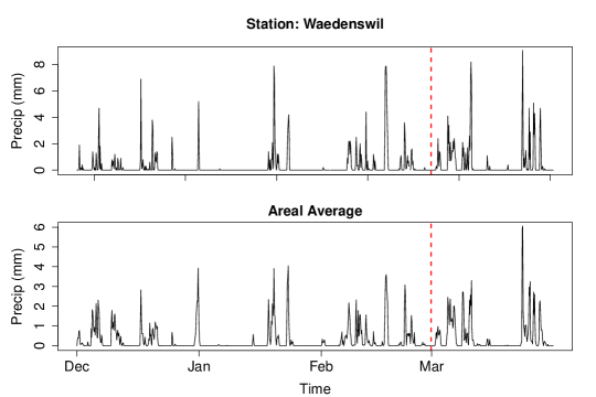
Figure 6: Precipitation (mm) versus time, for one station and averaged over all stations.

The NWP model forecasts are deterministic and ensembles are not available in our case. However, the extension to use an ensemble instead of just one member can be easily done. One can include all the ensemble members in the regression part of the model. Or, in the case of exchangeable members, one can use the location and the spread of the ensemble.

5.2 Precipitation Model for Postprocessing

The model presented in the following is a Bayesian hierarchical model (BHM). It uses the SPDE based spatio-temporal Gaussian process $\xi(t,{\boldsymbol{s}})$ presented in Section 3 at the process level. At the data stage, a mixture model adapted to the nature of precipitation is used. A characteristic feature of precipitation is that its distribution consists of a discrete component, indicating occurrence of precipitation, and a continuous one, determining the amount (see Figure 6). As a consequence, there are two basic statistical modeling approaches. The continuous and the discrete part are either modelled separately (Coe and Stern 1982; Wilks 1999) or together (Bell 1987; Wilks 1990; Bardossy and Plate 1992; Hutchinson 1995; Sansó and Guenni 2004). See, e.g., Sigrist et al. (2012) for a more extensive overview of precipitation models and for further details on the data model used below. Originally, the approach presented in the following goes back to Tobin (1958) who analyzed household expenditure on durable goods. For modeling precipitation, Stidd (1973) took up this idea and modified it by including a power transformation for the non-zero part so that the model can account for skewness. Sansó and Guenni (1999) develop Bayesian methods for the spatio-temporal analysis of rainfall using this skewed Tobit model, but in contrast to our application they do not explicitly account for temporal correlation and they use a much smaller spatial grid.

We denote the cumulative rainfall from time $t-1$ to $t$ at site ${\boldsymbol{s}}\in\mathbb{R}^{2}$ by $y(t,{\boldsymbol{s}})$ and assume that it depends on a latent Gaussian variable $w(t,{\boldsymbol{s}})$ through

$$\begin{split}y(t,{\boldsymbol{s}})&=0,\hskip 42.67912pt\text{if}~{}w(t,{\boldsymbol{s}})\leq 0,\\ &=w(t,{\boldsymbol{s}})^{\lambda},\hskip 11.38092pt\text{if}~{}w(t,{\boldsymbol{s}})>0,\\ \end{split}$$ (32)

where $\lambda>0$. A power transformation is needed since precipitation amounts are skewed and do not follow a truncated normal distribution. The latent Gaussian process $w(t,{\boldsymbol{s}})$ is interpreted as a precipitation potential.

The mean of the Gaussian process $w(t,{\boldsymbol{s}})$ is assumed to depend linearly on spatio-temporal covariates ${\boldsymbol{x}}(t,{\boldsymbol{s}})\in\mathbb{R}^{k}$. As shown below, this mean term basically consists of the NWP forecasts. Variation that is not explained by the linear term is modeled using the Gaussian process $\xi(t,{\boldsymbol{s}})$ and the unstructured term $\nu(t,{\boldsymbol{s}})$ for microscale variability and measurement errors. The spatio-temporal process $\xi(t,{\boldsymbol{s}})$ has two functions. First, it captures systematic errors of the NWP in space and time and can extrapolate them over time. Second, it accounts for structured variability so that the postprocessed forecast is probabilistic and its distribution sharp and calibrated.

To be more specific concerning the covariates, similarly to what appears in Berrocal et al. (2008), we include a transformed variable $y_{F}(t,{\boldsymbol{s}})^{1/\tilde{\lambda}}$ and an indicator variable $\mathbbm{1}_{\{y_{F}(t,{\boldsymbol{s}})=0\}}$ which equals $1$ if $y_{F}(t,{\boldsymbol{s}})=0$ and $0$ otherwise. $\tilde{\lambda}$ is determined by fitting the transformed Tobit model as in (32) to the marginal distribution of the rain data ignoring any spatio-temporal correlation. In doing so, we obtain $\tilde{\lambda}\approx 1.4$. $y_{F}(t,{\boldsymbol{s}})^{1/\tilde{\lambda}}$ is centered around zero by subtracting its overall mean $\overline{y}^{1/\tilde{\lambda}}_{F}$ in order to reduce posterior correlations. Thus, $w(t,{\boldsymbol{s}})$ equals

$$w(t,{\boldsymbol{s}})=b_{1}\left(y_{F}(t,{\boldsymbol{s}})^{1/\tilde{\lambda}}-\overline{y}_{F}^{1/\tilde{\lambda}}\right)+b_{2}\mathbbm{1}_{\{y_{F}(t,{\boldsymbol{s}})=0\}}+\xi(t,{\boldsymbol{s}})+\nu(t,{\boldsymbol{s}}).$$ (33)

An intercept is not included since the first Fourier term is constant in space. In our case, including an intercept term results in weak identifiability which slows down the convergence of the MCMC algorithm used for fitting. Note that in situations where the mean is large it is advisable to include an intercept, since the coefficient of the first Fourier term is constrained by the joint prior on ${\boldsymbol{\alpha}}$. Further, unidendifiability is unlikely to be a problem in these cases.

Concerning the spatio-temporal process $\xi(t,{\boldsymbol{s}})$, we apply padding. This means that we embed the $50\times 100$ grid in a rectangular $200\times 200$ grid. A brief prior investigation showed that the range parameters are relatively large in comparison to the spatial domain, and padding is therefore used in order to avoid spurious correlations due to periodicity. The NWP forecasts are not available on the extended $200\times 200$ domain, which means that, in principle, the process $w(t,{\boldsymbol{s}})$ can only be modeled on the $50\times 100$ grid where the covariates are available. To cope with this we use an incidence matrix ${\boldsymbol{H}}$ as in (30) to relate the process at the $200\times 200$ grid to the observation stations. As argued in Section 4.2, this then requires that we use a reduced dimensional Fourier expansion. I.e., instead of using $N=200^{2}$ basis functions, we only use $K<<N$ low-frequency Fourier terms. Since the observation stations are relatively scarce, one might argue that there is no information on spatial high frequencies of the NWP error, and that the high frequencies can be left out. In fact, this hypothesis gets confirmed by our analysis, see Figure 7.

Concerning prior distributions, for ${\boldsymbol{\theta}}=(\rho_{0},\sigma^{2},\zeta,\rho_{1},\gamma,\psi,\mu_{x},\mu_{y},\tau^{2})^{T}$, we use the priors presented in Section 4.3. The parameters ${\boldsymbol{b}}$ and $\lambda$, which are not included in ${\boldsymbol{\theta}}$, have improper, locally uniform priors on $\mathbb{R}$ and $\mathbb{R}_{+}$, respectively. In summary,

$$P[{\boldsymbol{b}},\lambda,{\boldsymbol{\theta}}]\propto\frac{1}{\sqrt{\sigma^{2}}\sqrt{\tau^{2}}\gamma}\mathbbm{1}_{\{-0.5\leq\mu_{x},\mu_{y}\leq 0.5\}}\mathbbm{1}_{\{0\leq\psi\leq\pi/2\}}\mathbbm{1}_{\{\lambda,\rho_{0},\rho_{1},\zeta,\sigma^{2},\tau^{2}\geq 0\}}\mathbbm{1}_{\{0.1\leq\gamma\leq 10\}}.$$

In addition, concerning ${\boldsymbol{\alpha}}(0)$, we choose to use the innovation distribution specified in (6) as initial distribution.

5.3 Fitting

Monte Carlo Markov Chain (MCMC) is used to sample from the posterior distribution $[{\boldsymbol{b}},\lambda,{\boldsymbol{\theta}},{\boldsymbol{\alpha}},{\boldsymbol{w}}|{\boldsymbol{y}}]$, where ${\boldsymbol{y}}$ denotes the set of all observations. We use what Neal and Roberts (2006) call a Metropolis within-Gibbs algorithm which alternates between blocked Gibbs (Gelfand and Smith 1990) and Metropolis (Metropolis et al. 1953; Hastings 1970) sampling steps.

We use the Metropolis-Hastings algorithm presented in Section 4.3 with the coefficients ${\boldsymbol{b}}$ being sampled jointly with ${\boldsymbol{\theta}}$ and ${\boldsymbol{\alpha}}$. Due to the non-Gaussian data model, additional Metropolis and Gibbs steps are required for $\lambda$ and for those points of ${\boldsymbol{w}}$ where the observed rainfall amount is zero and where observations are missing. We refer to Sigrist et al. (2012) for more details on the type of data augmentation approach that is used for doing this. We denote by ${\boldsymbol{w}}^{[0]}$ the values of ${\boldsymbol{w}}$ at those points where the observed rainfall is zero, $y(t,{\boldsymbol{s}})=0$. Analogously, we define ${\boldsymbol{w}}^{[m]}$ and ${\boldsymbol{w}}^{[+]}$ for the missing values and the values where a positive rainfall amount is observed, $y(t,{\boldsymbol{s}})>0$, respectively. The full conditionals of the censored ${\boldsymbol{w}}^{[0]}$ and missing points ${\boldsymbol{w}}^{[m]}$ are truncated and regular one-dimensional Gaussian distributions, respectively. Sampling from them is done in Gibbs steps. The transformation parameter $\lambda$ is sampled using a random walk Metropolis step. If a new value is accepted, ${\boldsymbol{w}}^{[+]}$ needs to be updated using the deterministic relation $w(t,{\boldsymbol{s}})=y(t,{\boldsymbol{s}})^{1/\lambda}$ due to (32). From these Gibbs and Metropolis steps, we obtain ${\boldsymbol{w}}$ consisting of simulated and transformed observed data. In the second part of the algorithm, we sample ${\boldsymbol{b}},{\boldsymbol{\theta}}$, and ${\boldsymbol{\alpha}}$ jointly from $[{\boldsymbol{b}},{\boldsymbol{\theta}},{\boldsymbol{\alpha}}|{\boldsymbol{w}}]$ using the algorithm presented in Section 4.3, where ${\boldsymbol{w}}$ acts as if it was the observed data. After a burn-in of $5,000$ iterations, we use $100,000$ samples from the Markov chain to characterize the posterior distribution. Convergence is monitored by inspecting trace plots.

5.4 Model Selection and Results

We use a reduced dimensional approach. The number of Fourier functions is determined based on predictive performance for the $240$ time points that were set aside. We start with models including only low spatial frequencies and add successively higher frequencies. In doing so, we only consider models that have the same resolution in each direction, i.e., we do not consider models that have higher frequency spatial basis functions in the east-west direction than in the north-south one.

In order to assess the performance of the predictions and to choose the number of basis functions to include, we use the continuous ranked probability score (CRPS) (Matheson and Winkler 1976). The CRPS is a strictly proper scoring rule (Gneiting and Raftery 2007) that assigns a numerical value to probabilistic forecasts and assesses calibration and sharpness simultaneously (Gneiting et al. 2007). It is defined as

$$CRPS(F,y)=\int_{-\infty}^{\infty}(F(x)-\mathbbm{1}_{\{y\leq x\}})^{2}dx,$$ (34)

where $F$ is the predictive cumulative distribution, $y$ is the observed realization, and $\mathbbm{1}$ denotes an indicator function. If a sample $y^{(1)},\dots,y^{(m)}$ from $F$ is available, it can be approximated by

$$\frac{1}{m}\sum_{i=1}^{m}|y^{(i)}-y|-\frac{1}{2m^{2}}\sum_{i,j=1}^{m}|y^{(i)}-y^{(j)}|.$$ (35)

Ideally, one would run the full MCMC algorithm at each time point $t\geq 720$, including all data up to the point, and obtain predictive distributions from this. Since this is rather time consuming, we make the following approximation. We assume that the posterior distribution of the “primary” parameters ${\boldsymbol{\theta}}$, ${\boldsymbol{b}}$, and $\lambda$ given ${\boldsymbol{y}}_{1:t}=\{{\boldsymbol{y}}_{1},\dots,{\boldsymbol{y}}_{t}\}$ is the same for all $t\geq 720$. That is, we neglect the additional information that the observations in March provide about the primary parameters. Thus, the posterior distributions of the primary parameters are calculated only once, namely on the data set from December 2008 to February 2009. The assumption that the posterior of the primary parameters does not change with additional data may be questionable over longer time periods and when one moves away from the time period from which data is used to obtain the posterior distribution. But since all our data lies in the winter season, we think that this assumption is reasonable. If longer time periods are considered, one could use sliding training windows or model the primary parameters as non-stationary using a temporal evolution.

For each time point $t\geq 720$, we make up to $8$ steps ahead forecasts corresponding to 24 hours. I.e., we sample from the predictive distribution of ${\boldsymbol{y}}^{*}_{t+k}$, $k=1,\dots 8$, given ${\boldsymbol{y}}_{1:t}=\{{\boldsymbol{y}}_{1},\dots,{\boldsymbol{y}}_{t}\}$.

Figure 7: Comparison of different statistical models using the continuous ranked probability score (CRPS). On the left are CRPSs of station specific forecasts and on the right are CRPSs of areal forecasts. $K$ denotes the number of basis functions used in the model. “Sep” denotes the separable model with $K=29$ Fourier terms. The unit of the CRPS is mm.

In Figure 7, the average CRPS of the pointwise predictions and the areal predictions are shown for the different statistical models. In the left plot, the mean is taken over all stations and lead times, whereas the areal version is an average over all lead times. This is done for the models with different numbers of basis functions used. Models including only a few low-frequency Fourier terms perform worse. Then the CRPS decreases successively. The model based on including $K=29$ Fourier functions performs best. After this, adding higher frequencies results into lower predictive performance. We interpret this results in the way that the observation data does not allow for resolving high frequencies in the error term between the forecasted and observed precipitation. Note that high frequencies of the precipitation process itself are accounted for by the forecast $y_{F}$. For comparison, we also fit a separable model which is obtained by setting ${\boldsymbol{\mu}}={\boldsymbol{0}}$ and ${\boldsymbol{\Sigma}}^{-1}={\boldsymbol{0}}_{2,2}$. Concerning the number of Fourier functions, we use $K=29$ different Fourier terms. The separable model clearly performs worse than the model with a non-separable covariance structure. Based on these findings, we decided to use the model with $29$ cosine and sine functions.

Table 1: Posterior medians and 95 $\%$ credible intervals for the SPDE based spatio-temporal model presented in Section 3 with $K=29$ Fourier terms.

	Median	2.5 %	97.5 %
$\rho_{0}$	25.4	18.8	32.4
$\sigma^{2}$	0.838	0.727	0.994
$\zeta$	0.00655	0.000395	0.0156
$\rho_{1}$	48.8	42.1	57.1
$\gamma$	4.33	3.34	6.01
$\psi$	0.557	0.49	0.617
$\mu_{x}$	6.73	0.688	12.9
$\mu_{y}$	-4.19	-8.55	-0.435
$\tau^{2}$	0.307	0.288	0.327
$b_{1}$	0.448	0.414	0.481
$b_{2}$	-0.422	-0.5	-0.344
$\lambda$	1.67	1.64	1.7

Table 1 shows posterior medians as well as $95\%$ credible intervals for the different parameters. Note that the range parameters $\rho_{0}$ and $\rho_{1}$ as well as the drift parameters $\mu_{x}$ and $\mu_{y}$ have been transformed back from the unit $[0,1]$ scale to the original km scale. The posterior median of the variance $\sigma^{2}$ of the innovations of the spatio-temporal process is around $0.8$. Compared to this, the nugget variance being about $0.3$ is smaller. For the innovation range parameter $\rho_{0}$, we obtain a value of about $25$ km. And the range parameter $\rho_{1}$ that controls the amount of diffusion or, in other words, the amount of spatio-temporal interaction, is approximately $49$ km. With $\gamma$ and $\psi$ being around $4$ and $0.6$, respectively, we observe anisotropy in the south-west to north-east direction. This is in line with the orography of the region, as the majority of the grid points lies between two mountain ranges: the Jura to the north-west and the Alps to the south-east. The drift points to the south-east, both parameters being rather small though. Further, the damping parameter $\zeta$ has a posterior median of about $0.01$.

Table 2: Comparison of NWP model and statistically postprocessed forecasts (’Stat PP’) using the mean absolute error (MAE). ’Static’ denotes the constant forecast obtained by using the most recently observed data. The unit of the MAE is mm.

	Stat PP	NWP	Static
Stationwise	0.359	0.485	0.594
Areal	0.303	0.387	0.489

Next, we compare the performance of the postprocessed forecasts with the ones from the NWP model. In addition to the temporal cross-validation, we do the following cross-validation in space and time. We first remove six randomly selected stations from the data, fit the latent process to the remaining stations, and evaluate the forecasts at the stations left out. Concerning the primary parameters, i.e., all parameters except the latent process, we use the posterior obtained from the full data including all stations. This is done for computational simplicity and since this posterior is not very sensitive when excluding a few stations (results not reported). Since the NWP produces 8 step ahead predictions once a day, we only consider statistical forecasts starting at 0:00UTC. This is in contrast to the above comparison of the different statistical models for which 8 step ahead predictions were made at all time points and not just once for each day. We use the mean absolute error (MAE) for evaluating the NWP forecasts. In order to be consistent, we also generate point forecasts from the statistical predictive distributions by using medians, and then calculate the MAE for these point forecasts. In Table 2, the results are reported. For comparison, we also give the score for the static forecast that is obtained by using the most recently observed data. The postprocessed forecasts clearly perform better than the raw NWP forecasts. In addition, the postprocessed forecasts have the advantage that they provide probabilistic forecasts quantifying prediction uncertainty.

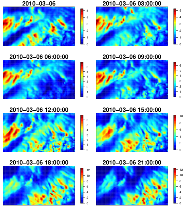
(a) NWP

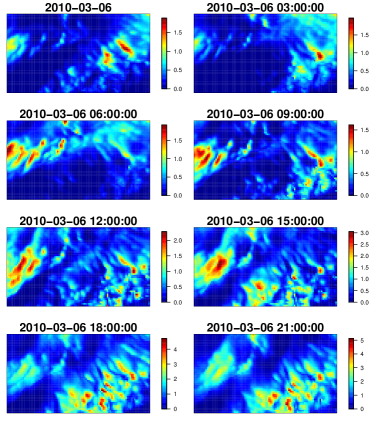
(b) Median

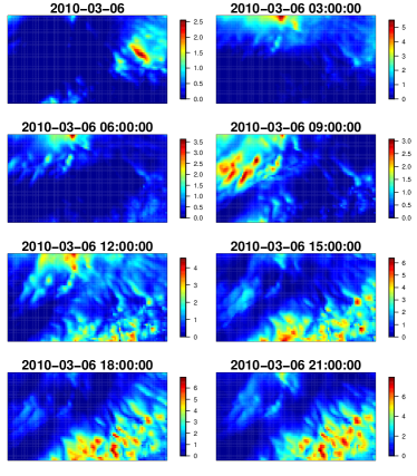
(c) One sample

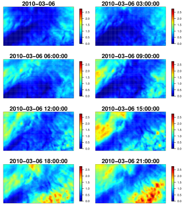
(d) Quartile difference

Figure 8: Illustration of postprocessed spatio-temporal precipitation fields for the period $t=761,\dots,768$. The figure shows the NWP forecasts (a), pointwise medians of the predictive distribution (b), one sample from the predictive distribution (c), and the differences between the third quartile and the median of the predictive distribution (d). All quantities are in mm. Note that the scales are different in different figures.

The statistical model produces a joint spatio-temporal predictive distribution that is spatially highly resolved. To illustrate the use of the model, we show several quantities in Figure 8. We consider the time point $t=760$ and calculate predictive distributions over the next 24 hours. Predicted fields for the period $t=761,\dots,768$ from the NWP are shown in the top left corner. On the right of it are pointwise medians obtained from the statistical forecasts. This is a period during which the NWP predicts too much rainfall compared to the observed data (results not shown). The figure shows how the statistical model corrects for this. For illustration, we also show one sample from the predictive distribution. To quantify prediction uncertainty, the difference between the third quartile and the median of the predictive distribution is plotted. These plots again show the growing uncertainty with increasing lead time. Other quantities of interest (not shown here), that can be easily obtained, include probabilities of precipitation occurrence or various quantiles of the distribution.

6   Conclusion

We present a spatio-temporal model and corresponding efficient algorithms for doing statistical inference for large data sets. Instead of using the covariance function, we propose to use a Gaussian process defined trough an SPDE. The SPDE is solved using Fourier functions, and we have given a bound on the precision of the approximate solution. In the spectral space, one can use computationally efficient statistical algorithms whose computational costs grow linearly with the dimension, the total computational costs being dominated by the fast Fourier transform. The space-time Gaussian process defined through the advection-diffusion SPDE has a nonseparable covariance structure and can be physically motivated. The model is applied to postprocessing of precipitation forecasts for northern Switzerland. The postprocessed forecasts clearly outperform the raw NWP predictions. In addition, they have the advantage that they quantify prediction uncertainty.

In our analysis, we considered cumulative rainfall over 3 hours, both in the NWP forecasts and in the station data. It would be interesting to formulate a model which can describe different accumulation periods in a coherent way and is still computationally feasible. Another interesting direction for further research would be to extend the SPDE based model to allow for spatial non-stationarity. For instance, the deformation method of Sampson and Guttorp (1992), where the process is assumed to be stationary in a transformed space and non-stationary in the original domain, might be a potential way. Since the operators of the SPDE are local, one can define the SPDE on general manifolds and, in particular, on the sphere (see, e.g., Lindgren et al. (2011)). Future research will show to which extent spectral methods can still be used in practice.

References

- Abramowitz and Stegun (1964) Abramowitz, M. and I. A. Stegun (1964). Handbook of Mathematical Functions. New York: Dover Publications.
- Anderson and Moore (1979) Anderson, B. D. O. and J. B. Moore (1979). Optimal filtering / Brian D. O. Anderson, John B. Moore. Prentice-Hall, Englewood Cliffs, N.J.
- Antolik (2000) Antolik, M. S. (2000). An overview of the national weather service’s centralized statistical quantitative precipitation forecasts. Journal of Hydrology 239(1-4), 306 – 337.
- Applequist et al. (2002) Applequist, S., G. E. Gahrs, R. L. Pfeffer, and X.-F. Niu (2002, August). Comparison of methodologies for probabilistic quantitative precipitation forecasting. Weather and Forecasting 17, 783–799.
- Aune and Simpson (2012) Aune, E. and D. Simpson (2012). The use of systems of stochastic PDEs as priors for multivariate models with discrete structures. arXiv preprint arXiv:1208.1717.
- Banerjee et al. (2004) Banerjee, S., B. P. Carlin, and A. E. Gelfand (2004). Hierarchical Modeling and Analysis for Spatial Data. Monographs on Statistics and Applied Probability. Chapman and Hall/CRC.
- Banerjee et al. (2008) Banerjee, S., A. E. Gelfand, A. O. Finley, and H. Sang (2008). Gaussian predictive process models for large spatial data sets. Journal Of The Royal Statistical Society Series B 70(4), 825–848.
- Bardossy and Plate (1992) Bardossy, A. and E. Plate (1992). Space-time model for daily rainfall using atmospheric circulation patterns. Water Resources Research 28(5), 1247–1259.
- Bell (1987) Bell, T. (1987, AUG 20). A space-time stochastic model of rainfall for satellite remote-sensing studies. Journal of Geophysical Research 92(D8), 9631–9643.
- Berrocal et al. (2008) Berrocal, V. J., A. E. Raftery, and T. Gneiting (2008, DEC). Probabilistic quantitative precipitation field forecasting using a two-stage spatial model. Annals of Applied Statistics 2(4), 1170–1193.
- Borgman et al. (1984) Borgman, L., M. Taheri, and R. Hagan (1984). Three-dimensional frequency-domain simulations of geological variables. In G. Verly (Ed.), Geostatistics for Natural Resources Characterization, pp. 517–541. D. Reidel.
- Bremnes (2004) Bremnes, B. J. (2004). Probabilistic forecasts of precipitation in terms of quantiles using NWP model output. Monthly Weather Review 132, 338–347.
- Bronson and Costa (2007) Bronson, R. and G. B. Costa (2007). Linear Algebra: An Introduction. Academic Press.
- Brooks et al. (2011) Brooks, S., A. Gelman, G. Jones, and X. Meng (2011). Handbook of Markov Chain Monte Carlo. Chapman & Hall/CRC Handbooks of Modern Statistical Methods. Taylor & Francis.
- Brown et al. (2000) Brown, P. E., K. F. Karesen, G. O. Roberts, and S. Tonellato (2000). Blur-generated non-separable space-time models. Journal of the Royal Statistical Society. Series B (Statistical Methodology) 62(4), 847–860.
- Cameletti et al. (2013) Cameletti, M., F. Lindgren, D. Simpson, and H. Rue (2013). Spatio-temporal modeling of particulate matter concentration through the SPDE approach. AStA Advances in Statistical Analysis 79, 109–131.
- Carter and Kohn (1994) Carter, C. K. and R. Kohn (1994). On Gibbs sampling for state space models. Biometrika 81(3), 541–553.
- Coe and Stern (1982) Coe, R. and R. Stern (1982). Fitting models to daily rainfall data. Journal of Applied Meteorology 21(7), 1024–1031.
- Cooley and Tukey (1965) Cooley, J. W. and J. W. Tukey (1965). An algorithm for the machine calculation of complex Fourier series. Math. Comp. 19, 297–301.
- Cramér and Leadbetter (1967) Cramér, H. and M. R. Leadbetter (1967). Stationary and related stochastic processes. Sample function properties and their applications. New York: John Wiley & Sons Inc.
- Cressie and Huang (1999) Cressie, N. and H.-C. Huang (1999). Classes of nonseparable, spatio-temporal stationary covariance functions. Journal of the American Statistical Association 94(448), 1330–1340.
- Cressie and Johannesson (2008) Cressie, N. and G. Johannesson (2008). Fixed rank kriging for very large spatial data sets. Journal of the Royal Statistical Society: Series B (Statistical Methodology) 70(1), 209–226.
- Cressie and Wikle (2011) Cressie, N. and C. K. Wikle (2011). Statistics for spatio-temporal data. Wiley Series in Probability and Statistics. John Wiley Sons, Inc.
- Duan et al. (2009) Duan, J. A., A. E. Gelfand, and C. Sirmans (2009). Modeling space-time data using stochastic differential equations. Bayesian Analysis 4(4), 733–758.
- Dudgeon and Mersereau (1984) Dudgeon, D. E. and R. M. Mersereau (1984). Multidimensional digital signal processing. Prentice-Hall.
- Eidsvik et al. (2012) Eidsvik, J., B. Shaby, B. Reich, M. Wheeler, and J. Niemi (2012). Estimation and prediction in spatial models with block composite likelihoods using parallel computing. Technical report, Department of Mathematical Sciences, NTNU. http://www.math.ntnu.no/joeid/ESRWN.pdf.
- Folland (1992) Folland, G. B. (1992). Fourier analysis and its applications. The Wadsworth & Brooks/Cole Mathematics Series. Pacific Grove, CA: Wadsworth & Brooks/Cole Advanced Books & Software.
- Friederichs and Hense (2007) Friederichs, P. and A. Hense (2007). Statistical downscaling of extreme precipitation events using censored quantile regression. Monthly Weather Review 135, 2365–2378.
- Frühwirth-Schnatter (1994) Frühwirth-Schnatter, S. (1994). Data augmentation and dynamic linear models. Journal of Time Series Analysis 15, 183–202.
- Fuentes (2007) Fuentes, M. (2007). Approximate likelihood for large irregularly spaced spatial data. Journal of the American Statistical Association 102, 321–331.
- Furrer et al. (2006) Furrer, R., M. G. Genton, and D. Nychka (2006). Covariance tapering for interpolation of large spatial datasets. Journal of Computational and Graphical Statistics 15(3), 502–523.
- Gelfand et al. (2005) Gelfand, A. E., S. Banerjee, and D. Gamerman (2005). Spatial process modelling for univariate and multivariate dynamic spatial data. Environmetrics 16(5), 465–479.
- Gelfand and Smith (1990) Gelfand, A. E. and A. F. M. Smith (1990). Sampling-based approaches to calculating marginal densities. Journal of the American Statistical Association 85(410), 398–409.
- Gelman (2006) Gelman, A. (2006). Prior distributions for variance parameters in hierarchical models. Bayesian Analysis 1, 1–19.
- Gilks et al. (1996) Gilks, W. R., S. Richardson, and D. J. Spiegelhalter (1996). Markov Chain Monte Carlo in Practice. London: Chapman and Hall.
- Gneiting (2002) Gneiting, T. (2002). Nonseparable, stationary covariance functions for space-time data. Journal of the American Statistical Association 97(458), 590–600.
- Gneiting et al. (2007) Gneiting, T., F. Balabdaoui, and A. E. Raftery (2007). Probabilistic forecasts, calibration and sharpness. Journal Of The Royal Statistical Society Series B 69(2), 243–268.
- Gneiting et al. (2007) Gneiting, T., M. G. Genton, and P. Guttorp (2007). Geostatistical space-time models, stationarity, separability and full symmetry. In B. Finkenstädt, L. Held, and V. Isham (Eds.), Modelling Longitudinal and Spatially Correlated Data, Volume 107 of Monographs on Statistics and Applied Probability, pp. 151–175. Boca Raton: Chapman Hall/CRC.
- Gneiting and Raftery (2005) Gneiting, T. and A. E. Raftery (2005). Weather forecasting with ensemble methods. Science 310(5746), 248–249.
- Gneiting and Raftery (2007) Gneiting, T. and A. E. Raftery (2007). Strictly proper scoring rules, prediction, and estimation. Journal of the American Statistical Association 102, 359–378.
- Golightly and Wilkinson (2008) Golightly, A. and D. Wilkinson (2008). Bayesian inference for nonlinear multivariate diffusion models observed with error. Computational Statistics Data Analysis 52(3), 1674 – 1693.
- Gottlieb and Orszag (1977) Gottlieb, D. and S. A. Orszag (1977). Numerical analysis of spectral methods: theory and applications. Philadelphia, Pa.: Society for Industrial and Applied Mathematics.
- Haberman (2004) Haberman, R. (2004). Applied partial differential equations: with Fourier series and boundary value problems. Pearson Prentice Hall.
- Hamill and Colucci (1997) Hamill, T. M. and S. J. Colucci (1997). Verification of Eta RSM short-range ensemble forecasts. Monthly Weather Review 125, 1312–1327.
- Hamill et al. (2004) Hamill, T. M., J. S. Whitaker, and X. Wei (2004). Ensemble reforecasting: Improving medium-range forecast skill using retrospective forecasts. Monthly Weather Review 132, 1434–1447.
- Handcock and Stein (1993) Handcock, M. S. and M. L. Stein (1993). A Bayesian analysis of kriging. Technometrics 35(4), 403–410.
- Hastings (1970) Hastings, W. K. (1970, April). Monte Carlo sampling methods using Markov chains and their applications. Biometrika 57(1), 97–109.
- Heine (1955) Heine, V. (1955). Models for two-dimensional stationary stochastic processes. Biometrika 42(1/2), pp. 170–178.
- Hu et al. (2013) Hu, X., D. S. Lindgren, H. Rue, et al. (2013). Multivariate gaussian random fields using systems of stochastic partial differential equations. arXiv preprint arXiv:1307.1379.
- Huang and Hsu (2004) Huang, H.-C. and N.-J. Hsu (2004). Modeling transport effects on ground-level ozone using a non-stationary space-time model. Environmetrics 15(3), 251–268.
- Hutchinson (1995) Hutchinson, M. (1995). Stochastic space-time weather models from ground-based data. Agricultural and Forest Meteorology 73(3-4), 237–264.
- Johannesson et al. (2007) Johannesson, G., N. Cressie, and H.-C. Huang (2007). Dynamic multi-resolution spatial models. Environmental and Ecological Statistics 14, 5–25.
- Jones and Zhang (1997) Jones, R. and Y. Zhang (1997). Models for continuous stationary space-time processes. In T. Gregoire, D. R. Brillinger, P. J. Diggle, E. Russek-Cohen, W. G. Warren, and R. Wolfinger (Eds.), Modelling Longitudinal and Spatially Correlated Data, Volume 122 of Lecture Notes in Statistics, pp. 289–298. New-York: Springer-Verlag.
- Kleiber et al. (2011) Kleiber, W., A. E. Raftery, and T. Gneiting (2011). Geostatistical model averaging for locally calibrated probabilistic quantitative precipitation forecasting. Journal of the American Statistical Association 106(496), 1291–1303.
- Krzysztofowicz and Maranzano (2006) Krzysztofowicz, R. and C. J. Maranzano (2006). Bayesian processor of output for probabilistic quantitative precipitation forecasting. Technical report, Department of Systems Engineering and Deptartment of Statistics, University Virginia.
- Künsch (2001) Künsch, H. R. (2001). State space and hidden Markov models. In Complex stochastic systems (Eindhoven, 1999), Volume 87 of Monogr. Statist. Appl. Probab., pp. 109–173. Chapman & Hall/CRC, Boca Raton, FL.
- Lindgren et al. (2011) Lindgren, F., H. Rue, and J. Lindstrom (2011). An explicit link between Gaussian fields and Gaussian Markov random fields: the stochastic partial differential equation approach. Journal of the Royal Statistical Society: Series B (Statistical Methodology) 73(4), 423–498.
- Ma (2003) Ma, C. (2003). Families of spatio-temporal stationary covariance models. Journal of Statistical Planning and Inference 116(2), 489 – 501.
- Malmberg et al. (2008) Malmberg, A., A. Arellano, D. P. Edwards, N. Flyer, D. Nychka, and C. Wikle (2008). Interpolating fields of carbon monoxide data using a hybrid statistical-physical model. The Annals of Applied Statistics 2(4), 1231–1248.
- Matheson and Winkler (1976) Matheson, J. E. and R. L. Winkler (1976). Scoring rules for continuous probability distributions. Management Science 22(10), pp. 1087–1096.
- Metropolis et al. (1953) Metropolis, N., A. W. Rosenbluth, M. N. Rosenbluth, A. H. Teller, and E. Teller (1953). Equation of state calculations by fast computing machines. The Journal of Chemical Physics 21(6), 1087–1092.
- Neal and Roberts (2006) Neal, P. and G. Roberts (2006). Optimal scaling for partially updating MCMC algorithms. The Annals of Applied Probability 16(2), pp. 475–515.
- Nychka et al. (2002) Nychka, D., C. Wikle, and J. A. Royle (2002). Multiresolution models for nonstationary spatial covariance functions. Statistical Modeling 2(4), 315–331.
- Paciorek (2007) Paciorek, C. J. (2007). Bayesian smoothing with Gaussian processes using Fourier basis functions in the spectralGP package. Journal of Statistical Software 19(2), 1–38.
- Paciorek and Schervish (2006) Paciorek, C. J. and M. J. Schervish (2006). Spatial modelling using a new class of nonstationary covariance functions. Environmetrics 17(5), 483–506.
- Palmer (2002) Palmer, T. N. (2002). The economic value of ensemble forecasts as a tool for risk assessment: From days to decades. Quarterly Journal of the Royal Meteorological Society 128(581), 747–774.
- Pedlosky (1987) Pedlosky, J. (1987). Geophysical Fluid Dynamics. Springer study edition. Springer-Verlag.
- Ramírez et al. (2005) Ramírez, M. C. V., H. F. de Campos Velho, and N. J. Ferreira (2005). Artificial neural network technique for rainfall forecasting applied to the Sao Paulo region. Journal of Hydrology 301(1-4), 146 – 162.
- Robert and Casella (2004) Robert, C. P. and G. Casella (2004). Monte Carlo Statistical Methods, Second Edition (2 ed.). Springer Texts in Statistics. Spring Street, New York, NY 10013, USA: Springer Science and Business Media Inc.
- Roberts and Rosenthal (2001) Roberts, G. O. and J. S. Rosenthal (2001). Optimal scaling for various Metropolis-Hastings algorithms. Statistical Science 16(4), pp. 351–367.
- Roberts and Rosenthal (2009) Roberts, G. O. and J. S. Rosenthal (2009). Examples of adaptive MCMC. Journal of Computational and Graphical Statistics 18(2), 349–367.
- Roberts and Stramer (2001) Roberts, G. O. and O. Stramer (2001). On inference for partially observed nonlinear diffusion models using the Metropolis-Hastings algorithm. Biometrika 88(3), pp. 603–621.
- Royle and Wikle (2005) Royle, J. A. and C. K. Wikle (2005). Efficient statistical mapping of avian count data. Environmental and Ecological Statistics 12, 225–243.
- Rue and Held (2005) Rue, H. and L. Held (2005). Gaussian Markov random fields, Volume 104 of Monographs on Statistics and Applied Probability. Chapman & Hall/CRC, Boca Raton, FL. Theory and applications.
- Rue and Tjelmeland (2002) Rue, H. and H. Tjelmeland (2002). Fitting Gaussian Markov random fields to Gaussian fields. Scandinavian Journal of Statistics 29(1), 31–49.
- Sampson and Guttorp (1992) Sampson, P. D. and P. Guttorp (1992). Nonparametric estimation of nonstationary spatial covariance structure. Journal of the American Statistical Association 87(417), 108–119.
- Sansó and Guenni (1999) Sansó, B. and L. Guenni (1999). Venezuelan rainfall data analysed by using a Bayesian space-time model. Journal of the Royal Statistical Society. Series C (Applied Statistics) 48(Part 3), 345–362.
- Sansó and Guenni (2004) Sansó, B. and L. Guenni (2004). A Bayesian approach to compare observed rainfall data to deterministic simulations. Environmetrics 15(6), 597–612.
- Shumway and Stoffer (2000) Shumway, R. H. and D. S. Stoffer (2000). Time series analysis and its applications. Springer Texts in Statistics. New York: Springer-Verlag.
- Sigrist et al. (2012) Sigrist, F., H. R. Künsch, and W. A. Stahel (2012). A dynamic nonstationary spatio-temporal model for short term prediction of precipitation. Ann. Appl. Statist. 6(4), 1452–1477.
- Sigrist et al. (2012) Sigrist, F., H. R. Künsch, and W. A. Stahel (2012). spate: an R package for statistical modeling with SPDE based spatio-temporal Gaussian processes. Technical report, Seminar for Statistics, ETH Zurich. http://stat.ethz.ch/people/sigrist/spate.pdf.
- Simpson et al. (2012) Simpson, D., F. Lindgren, and H. Rue (2012). In order to make spatial statistics computationally feasible, we need to forget about the covariance function. Environmetrics 23(1), 65–74.
- Sloughter et al. (2007) Sloughter, J. M., A. E. Raftery, T. Gneiting, and C. Fraley (2007, SEP). Probabilistic quantitative precipitation forecasting using Bayesian model averaging. Monthly Weather Review 135(9), 3209–3220.
- Smith and Roberts (1993) Smith, A. F. M. and G. O. Roberts (1993). Bayesian computation via the Gibbs sampler and related Markov chain Monte Carlo methods. Journal of the Royal Statistical Society. Series B (Methodological) 55(1), 3–23.
- Solna and Switzer (1996) Solna, K. and P. Switzer (1996). Time trend estimation for a geographic region. Journal of the American Statistical Association 91(434), 577–589.
- Stein (1999) Stein, M. L. (1999). Interpolation of spatial data, Some theory for Kriging. Springer Series in Statistics. New York: Springer-Verlag.
- Stein (2005) Stein, M. L. (2005, March). Space-time covariance functions. Journal of the American Statistical Association 100, 310–321.
- Stein (2008) Stein, M. L. (2008). A modeling approach for large spatial datasets. Journal of the Korean Statistical Society 37(1), 3 – 10.
- Stein et al. (2004) Stein, M. L., Z. Chi, and L. J. Welty (2004). Approximating likelihoods for large spatial data sets. Journal of the Royal Statistical Society: Series B (Statistical Methodology) 66(2), 275–296.
- Stensrud and Yussouf (2007) Stensrud, D. J. and N. Yussouf (2007). Reliable probabilistic quantitative precipitation forecasts from a short-range ensemble forecasting system. Weather and Forecasting 22, 2–17.
- Steppeler et al. (2003) Steppeler, J., G. Doms, U. Schättler, H. W. Bitzer, A. Gassmann, U. Damrath, and G. Gregoric (2003). Meso-gamma scale forecasts using the nonhydrostatic model LM. Meteorology and Atmospheric Physics 82, 75–96.
- Stidd (1973) Stidd, C. K. (1973). Estimating the precipitation climate. Water Resources Research 9, 1235–1241.
- Storvik et al. (2002) Storvik, G., A. Frigessi, and D. Hirst (2002). Stationary space-time Gaussian fields and their time autoregressive representation. Stat. Model. 2(2), 139–161.
- Stroud et al. (2010) Stroud, J. R., M. L. Stein, B. M. Lesht, D. J. Schwab, and D. Beletsky (2010). An ensemble Kalman filter and smoother for satellite data assimilation. Journal of the American Statistical Association 105(491), 978–990.
- Tobin (1958) Tobin, J. (1958). Estimation of relationships for limited dependent variables. Econometrica 26, 24–36.
- Vecchia (1988) Vecchia, A. V. (1988). Estimation and model identification for continuous spatial processes. Journal of the Royal Statistical Society. Series B (Methodological) 50(2), pp. 297–312.
- Vivar and Ferreira (2009) Vivar, J. C. and M. A. R. Ferreira (2009). Spatiotemporal models for gaussian areal data. Journal of Computational and Graphical Statistics 18(3), 658–674.
- Whittle (1954) Whittle, P. (1954). On stationary processes in the plane. Biometrika 41(3/4), pp. 434–449.
- Whittle (1962) Whittle, P. (1962). Topographic correlation, power-law covariance functions, and diffusion. Biometrika 49(3/4), pp. 305–314.
- Whittle (1963) Whittle, P. (1963). Stochastic processes in several dimensions. Bull. Inst. Internat. Statist. 40, 974–994.
- Wikle (2010) Wikle, C. (2010). Low-rank representations for spatial processes. In Handbook of Spatial Statistics, pp. 107–118. Chapman Hall/CRC Handbooks of Modern Statistical Methods.
- Wikle and Hooten (2010) Wikle, C. and M. Hooten (2010). A general science-based framework for dynamical spatio-temporal models. TEST 19, 417–451.
- Wikle (2002) Wikle, C. K. (2002). A kernel-based spectral model for non-gaussian spatio-temporal processes. Statistical Modelling 2(4), 299–314.
- Wikle (2003) Wikle, C. K. (2003). Hierarchical Bayesian models for predicting the spread of ecological processes. Ecology 84(6), pp. 1382–1394.
- Wikle et al. (1998) Wikle, C. K., L. M. Berliner, and N. Cressie (1998). Hierarchical Bayesian space-time models. Environmental and Ecological Statistics 5, 117–154.
- Wikle and Cressie (1999) Wikle, C. K. and N. Cressie (1999). A dimension-reduced approach to space-time Kalman filtering. Biometrika 86(4), 815–829.
- Wikle et al. (2001) Wikle, C. K., R. F. Milliff, D. Nychka, and L. M. Berliner (2001). Spatiotemporal hierarchical bayesian modeling: Tropical ocean surface winds. Journal of the American Statistical Association 96(454), 382–397.
- Wilks (1990) Wilks, D. (1990). Maximum likelihood estimation for the gamma distribution using data containing zeros. Journal of Climate 3(12), 1495–1501.
- Wilks (1999) Wilks, D. (1999). Multisite downscaling of daily precipitation with a stochastic weather generator. Climate Research 11(2), 125–136.
- Xu and Wikle (2007) Xu, K. and C. K. Wikle (2007). Estimation of parameterized spatio-temporal dynamic models. Journal of Statistical Planning and Inference 137(2), 567 – 588.
- Xu et al. (2005) Xu, K., C. K. Wikle, and N. I. Fox (2005). A kernel-based spatio-temporal dynamical model for nowcasting weather radar reflectivities. Journal of the American Statistical Association 100(472), 1133–1144.
- Yue et al. (2012) Yue, Y. R., D. Simpson, F. Lindgren, and H. Rue (2012). Bayesian adaptive smoothing spline using stochastic differential equations. arXiv preprint arXiv:1209.2013.
- Yussouf and Stensrud (2006) Yussouf, N. and D. J. Stensrud (2006). Prediction of near-surface variables at independent locations from a bias-corrected ensemble forecasting system. Monthly Weather Review 134, 3415–3424.
- Zheng and Aukema (2010) Zheng, Y. and B. H. Aukema (2010). Hierarchical dynamic modeling of outbreaks of mountain pine beetle using partial differential equations. Environmetrics 21(7-8), 801–816.