Scatter and bias in weak lensing selected clusters

Abstract

We examine scatter and bias in weak lensing selected clusters, employing both an analytic model of dark matter haloes and numerical mock data of weak lensing cluster surveys. We pay special attention to effects of the diversity of dark matter distributions within clusters. We find that peak heights of the lensing convergence map correlates rather poorly with the virial mass of haloes. The correlation is tighter for the spherical overdensity mass with a higher mean interior density (e.g., $M_{1000}$). We examine the dependence of the halo shape on the peak heights, and find that the root-mean-square scatter caused by the halo diversity scales linearly with the peak heights with the proportionality factor of $0.1-0.2$. The noise originated from the halo shape is found to be comparable to the source galaxy shape noise and the cosmic shear noise. We find the significant halo orientation bias, i.e., weak lensing selected clusters on average have their major axes aligned with the line-of-sight direction, and that the orientation bias is stronger for higher signal-to-noise ratio ($S/N$) peaks. We compute the orientation bias using an analytic triaxial halo model and obtain results quite consistent with the ray-tracing results. We develop a prescription to analytically compute the number count of weak lensing peaks taking into account all the main sources of scatters in peak heights. We find that the improved analytic predictions agree well with the simulation results for high $S/N$ peaks of $\nu\ga 5$. We also compare the expected number count with our weak lensing analysis results for 4 deg² of Subaru/Suprime-Cam observations and find a good agreement.

1 Introduction

Clusters of galaxies have been playing an important role in the field of cosmology. For instance, number counts of clusters have placed useful constraints on cosmological parameters (e.g., Vikhlinin et al., 2009b; Mantz et al., 2010; Rozo et al., 2010), and measurement of the dark matter distribution in clusters is useful for testing dark matter models (e.g., Dahle, 2006; Broadhurst et al., 2008; Mahdavi et al., 2008; Okabe & Umetsu, 2008; Oguri et al., 2009, 2010, 2012; Umetsu et al., 2009, 2011; Medezinski et al., 2010; Okabe et al., 2010). In most of these applications, the construction of homogeneous cluster samples and understanding selection biases are of fundamental importance, because an unknown bias can significantly affect the interpretation of the data.

Clusters of galaxies are identified by various techniques, including detections of galaxy concentrations in optical data, extended X-ray emissions (e.g., Böhringer et al., 2004; Vikhlinin et al., 2009a), the Sunyaev-Zel’dovich effect in the cosmic microwave background (e.g., Marriage et al, 2011; Reichardt et al., 2012), and dark matter concentrations in the weak lensing mass map (e.g., Miyazaki et al., 2002, 2007; Wittman et al, 2006; Gavazzi & Soucail, 2007; Schirmer et al., 2007; Kubo et al., 2009; Bellagamba et al., 2011; Shan et al., 2012; Kurtz et al., 2012). Each methodology has its own advantage and disadvantage. Among others, weak lensing technique is unique in the sense that it identifies clusters by searching for high peaks in the weak lensing mass map, and thus does not rely on physical state of the baryonic component (Schneider, 1996; Hamana, Takada, & Yoshida, 2004; Hennawi & Spergel, 2005; Maturi et al., 2005). Therefore, combining weak lensing cluster sample with samples selected by another method is beneficial not only for various cosmological applications but also for better understanding of cluster physics.

Recently Shan et al. (2012) reported 301 weak lensing high peaks located from 64 deg² data. Among those peaks, they confirmed 85 groups/clusters, which is the largest weak lensing cluster samples constructed to date (see also Miyazaki et al. (2007) and Schirmer et al. (2007)). Currently the size of weak lensing selected cluster sample is mainly limited by areas of optical imaging surveys. However, the situation is changing drastically in coming decade because there are several ongoing or planned wide field deep optical surveys including Dark Energy Survey, the KIlo-Degree Survey, Hyper Suprime-Cam, and Large Synoptic Survey Telescope. Thus in the near future, weak lensing selected cluster catalogues containing $\sim 10,000$ clusters will be available. It is therefore important to examine the selection function of the weak lensing selected cluster samples in order to take full advantage of these unique cluster catalogues.

The standard method for identifying clusters with weak lensing is to search for high peaks in the weak lensing mass map generated from weak lensing shear data with a carefully designed smoothing filter. Peaks above a given threshold are selected as cluster candidates. The peak height, which plays a central role in this study, is primarily determined by the mass and redshift of the dark matter halo of clusters (see e.g., Hamana, Takada, & Yoshida, 2004), but is also affected by the following three effects. The first is the noise arising from intrinsic shapes of source galaxies used for weak lensing shear measurements (galaxy shape noise). The second is the projection of structures along the line-of-sight. The third is the diversity of dark matter distributions in individual haloes. These effects are important in the sense that they induce the scatter and bias in the peak heights and hence in the resulting weak lensing selected cluster sample. While these effects were examined in literature to some extent (Hamana, Takada, & Yoshida, 2004; Hennawi & Spergel, 2005; Maturi et al., 2005; Tan & Fan, 2005; Pace et al., 2007; Fan, Shan & Liu, 2010; Marian, Smith, & Bernstein, 2010; Schmidt & Rozo, 2011; Dietrich et al., 2012), we revisit this problem with a particular emphasis on the scatter and bias produced by the diversity of dark matter distributions, using both analytic and numerical approaches.

The matter content of clusters is dominated by dark matter, which accounts for $\sim 80$ per cent of the mass of the universe. The dark matter distribution within dark matter haloes are investigated in detail using $N$-body simulations, which found that the radial profile of the dark matter halo is accurately described by an analytic form, the so-called NFW profile (Navarro, Frenk, & White, 1997). In this model, the matter distribution of haloes is characterized by two parameters, the mass and the concentration parameter. While it is known that there is a mean relationship between the mass and concentration parameter, the relation involves a large scatter among different haloes (e.g., Bullock et al., 2001). As pointed out by King & Mead (2011), the weak lensing peak height is sensitive to the halo concentration. Another important prediction of the current standard structure formation model is that the dark matter distribution in clusters is not spherically symmetric but is highly elongated (Jing & Suto, 2002). This non-sphericity of the dark matter distribution is known to have large impact on weak lensing measurements of clusters (Clowe, De Lucia, & King, 2004; Oguri et al., 2005; Gavazzi, 2005; Tan & Fan, 2005; Corless & King, 2009; Feroz & Hobson, 2012). Thus even the same mass haloes at the same redshift can produce largely different peak heights depending on the halo concentration and non-sphericity. This is exactly what we explore in this paper using a large set of mock data generated from gravitational lensing ray-tracing in $N$-body simulations.

The structure of this paper is as follows. In Section 2 we summarize the analytic description of cluster density distribution adopted in this paper and also summarize basics of cluster finding with weak lensing. We use a mock numerical simulation of weak lensing cluster survey which is detailed in Section 3. In Section 4 we investigate the scatter and bias in the weak lensing selected clusters, paying special attention to the influence of halo shape. We briefly compare the peak number count derived from the numerical mock data with our weak lensing analysis results of Subaru/Suprime-Cam observations in Section 5. Finally, summary and discussion are given in Section 6.

Throughout this paper we adopt the cosmological model with the matter density $\Omega_{M}=0.238$, baryon density $\Omega_{b}=0.042$, cosmological constant $\Omega_{\Lambda}=0.762$, spectral index $n_{s}=0.958$, the normalization of the matter fluctuation $\sigma_{8}=0.76$, and the Hubble parameter $h=0.732$, which are the best-fit cosmological parameters in the Wilkinson Microwave Anisotropy Probe (WMAP) third-year results (Spergel et al., 2007).

2 Analytic models of dark matter haloes

Let us first summarize the analytic models of dark matter distribution of clusters of galaxies and its weak lensing properties.

2.1 Dark matter distribution within haloes

We adopt the NFW model for the dark halo density profile which is given by (Navarro, Frenk, & White, 1997),

$$\rho_{\rm NFW}(r)=\frac{\rho_{s}}{(r/r_{s})(1+r/r_{s})^{2}}.$$ (1)

This model characterizes the dark matter distribution by two parameters: the density parameter $\rho_{s}$ and the scale radius $r_{s}$. It is customary to re-characterizes it by related parameters, the halo mass and the concentration parameter, which we define below.

The mass of haloes is not a uniquely defined quantity. One needs to choose proper definitions of masses depending on the purposes (White, 2001). In theoretical and observations studies, the virial mass $M_{\rm vir}$, which is defined such that the average density within the virial radius becomes equal to the nonlinear overdensity $\Delta_{\rm vir}$ computed using the spherical collapse model (see, e.g., Nakamura & Suto, 1997) times the mean matter density of the universe, has often been adopted. For the NFW model, the virial mass relates to $\rho_{s}$ and $r_{s}$ by

$$M_{\rm vir}=\frac{4\pi}{3}\Delta_{\rm vir}(z)\bar{\rho}_{m}(z)r_{\rm vir}^{3}=4\pi\rho_{s}r_{s}^{3}m_{\rm nfw}(c_{\rm vir}),$$ (2)

where $c_{\rm vir}$ is the so-called concentration parameter defined by

$$c_{\rm vir}\equiv\frac{r_{\rm vir}}{r_{s}}=\frac{1}{r_{s}}\left[\frac{3M_{\rm vir}}{4\pi\Delta_{\rm vir}(z)\bar{\rho}_{m}(z)}\right]^{1/3},$$ (3)

and $m_{\rm nfw}(c_{\rm vir})$ defined by

$$m_{\rm nfw}(c_{\rm vir})\equiv\int_{0}^{c_{\rm vir}}\frac{x}{(1+x)^{2}}dx=\ln(1+c_{\rm vir})-\frac{c_{\rm vir}}{1+c_{\rm vir}}.$$ (4)

The concentration parameter is known to be correlated with the halo mass and redshift. When necessary, we adopt the following relationship:

$$c_{\rm vir}(M_{\rm vir},z)=7.26\left(\frac{M_{\rm vir}}{10^{12}h^{-1}M_{\odot}}\right)^{-0.086}\left(1+z\right)^{-0.71},$$ (5)

which was derived from $N$-body simulations assuming the WMAP third year results (Macciò, Dutton, & van den Bosch, 2008), with the additional redshift dependence based on the simulation result of Duffy et al. (2008).

While the virial mass is a physically motivated definition of the halo mass, one can define halo masses using arbitrary values of overdensities. Specifically, one can use the spherical overdensity mass $M_{\Delta}$ defined by the mass contained within a radius $r_{\Delta}$ inside of which the mean interior density is $\Delta$ times the critical density

$$M_{\Delta}=\frac{4\pi}{3}\Delta\rho_{cr}(z)r_{\Delta}^{3}=4\pi\rho_{s}r_{s}^{3}m_{\rm nfw}(c_{\Delta}),$$ (6)

where

$$c_{\Delta}\equiv\frac{r_{\Delta}}{r_{s}}=\frac{1}{r_{s}}\left[\frac{3M_{\Delta}}{4\pi\Delta\rho_{cr}(z)}\right]^{1/3}.$$ (7)

In this paper, we also consider a triaxial halo model of Jing & Suto (2002) to investigate the effect of the halo triaxiality. In this model, the density profile given by eq. (1) is modified as

$$\rho_{\rm tri}(r)=\frac{\rho_{cd}}{(R/R_{0})(1+R/R_{0})^{2}},$$ (8)

$$R^{2}\equiv c^{2}\left(\frac{x^{2}}{a^{2}}+\frac{y^{2}}{b^{2}}+\frac{z^{2}}{c^{2}}\right)\;\;\;\;\;(a\leq b\leq c).$$ (9)

Jing & Suto (2002) derived the probability distribution of axis ratios $a/c$ and $b/c$ for haloes with a given mass and redshift from large $N$-body simulations. The lensing properties of the triaxial halo model were derived in Oguri, Lee, & Suto (2003) and Oguri & Keeton (2004), including projections of triaxial haloes along arbitrary directions, which we adopt in this paper. We study the effect of the halo triaxility on the properties of weak lensing selected clusters using the semi-analytic approach developed by Oguri & Blandford (2009). In this method, we generate a catalogue of haloes according to the mass function as well as axis ratio distributions of Jing & Suto (2002), and project each halo along random direction to compute the lensing properties. This allows us to generate a mock catalogue of weak lensing selected clusters based on the triaxial halo model.

2.2 Basics of weak lensing cluster finding

Here we summarize equations for weak lensing cluster finding which are directly relevant to the following analyses. For more detailed descriptions, see Schneider (1996); Bartelmann, King & Schneider (2001); Hamana, Takada, & Yoshida (2004); Hennawi & Spergel (2005); Maturi et al. (2005).

Let us first defined the weak lensing mass map which is the smoothed lensing convergence field ($\kappa$):

$${\cal K}(\mbox{\boldmath$\theta$})=\int d^{2}\mbox{\boldmath$\phi$}~{}\kappa(\mbox{\boldmath$\phi$}-\mbox{\boldmath$\theta$})U(|\mbox{\boldmath$\phi$}|),$$ (10)

where $U$ is the filter function to be specified below. The same quantity is obtained from the shear data by

$${\cal K}(\mbox{\boldmath$\theta$})=\int d^{2}\mbox{\boldmath$\phi$}~{}\gamma_{t}(\mbox{\boldmath$\phi$}:\mbox{\boldmath$\theta$})Q(|\mbox{\boldmath$\phi$}|),$$ (11)

where $\gamma_{t}(\mbox{\boldmath$\phi$}:\mbox{\boldmath$\theta$})$ is the tangential component of the shear at position $\phi$ relative to the point $\theta$, and $Q$ relates to $U$ by

$$Q(\theta)=\int_{0}^{\theta}d\theta^{\prime}~{}\theta^{\prime}U(\theta^{\prime})-U(\theta).$$ (12)

We consider $Q$ with a finite extent; in this case, one finds

$$U(\theta)=2\int_{\theta}^{\theta_{o}}d\theta^{\prime}~{}{{Q(\theta^{\prime})}\over{\theta^{\prime}}}-Q(\theta),$$ (13)

where $\theta_{o}$ is the outer boundary of the filter. Note that this is equivalent to set $U$ a finite compensated filter; that is, $\int^{\theta_{o}}d\theta~{}\theta~{}U(\theta)=0$ and $U(\theta)=0$ for $\theta>\theta_{o}$.

The basic idea of weak lensing cluster finding is to first construct a weak lensing mass map by applying eq. (11) to shear data, then to search for high peaks in the map which are plausible candidates of massive clusters. The root-mean-square (rms) noise coming from intrinsic ellipticity of galaxies (which we call the galaxy shape noise) is evaluated by (Schneider, 1996),

$$\sigma_{\rm shape}^{2}={{\sigma_{e}^{2}}\over{2n_{g}}}\int_{0}^{\theta_{o}}d\theta~{}\theta~{}Q^{2}(\theta),$$ (14)

where $\sigma_{e}$ is the rms value of intrinsic ellipticityies of galaxies and $n_{g}$ is the number density of galaxies. Throughout this paper, we take $\sigma_{e}=0.4$ and $n_{g}=30~{}{\rm arcmin}^{-2}$, which resembles the shape noise expected for the Hyper Suprime-Cam survey. The signal-to-noise ratio ($S/N$) of the weak lensing map is defined by the ratio between the peak height and $\sigma_{\rm shape}$,

$$\nu={{\cal K}\over{\sigma_{\rm shape}}}.$$ (15)

Figure 1: Three window functions considered in this paper are plotted. Top left: Absolute value of $U$ is shown, with negative $U$ being plotted by thin lines. The normalization is arbitrary. The convergence profile of the smoothly truncated NFW halo ($M_{\rm vir}=10^{14}h^{-1}M_{\odot}$, $z_{l}=0.3$, $z_{s}=1$) (Oguri & Hamana, 2011) is also plotted as the dotted line. Bottom left: $\theta^{2}\kappa_{\rm NFW}U$, which is the contribution to the ${\cal K}$ from the logarithmic $\theta$ interval, is plotted. Top right: The filter $Q$. The normalization is arbitrary. The tangential shear profile of the smoothly truncated NFW halo is also plotted. Bottom right: $\theta^{2}\gamma_{t}Q$, which is the contribution to the ${\cal K}$ from the logarithmic $\theta$ interval, is plotted.

In this paper we consider the following three filter functions. One is the truncated Gaussian (for $U$),

$$Q_{G}(\theta)={1\over{\pi\theta^{2}}}\left[1-\left(1+{{\theta^{2}}\over{\theta_{G}^{2}}}\right)\exp\left(-{{\theta^{2}}\over{\theta_{G}^{2}}}\right)\right],$$ (16)

for $\theta<\theta_{o}$ and $Q_{G}=0$ elsewhere. We take $\theta_{G}=1^{\prime}$, which is the value also adopted in Hamana, Takada, & Yoshida (2004), and $\theta_{o}=15^{\prime}$. The others filters have the following functional form, consisting of the power-law with outer exponential-cutoff,

$$Q_{PEXn}(\theta)={(\theta/\theta_{f})^{n}\over{\theta_{f}^{2}(1+a\theta/\theta_{f})^{(2+n)}}}\exp\left(-{{\theta^{2}}\over{2\theta_{e}^{2}}}\right).$$ (17)

We consider two cases: $(n,a)=(0,0.25)$ and $(1,0.7)$ which we call PEX0 and PEX1, respectively. The former mimics the filter function proposed by Maturi et al. (2005) designed for maximizing the $S/N$ of weak lensing peak by the NFW halo relative to noises coming from galaxy shape and cosmic structures, whereas the latter mimics the one proposed by Hennawi & Spergel (2005) which has a similar shape at the outer region but has less power on the inner region for suppressing the galaxy shape noise. We take $\theta_{f}=1^{\prime}$, $\theta_{e}=5^{\prime}$ and $\theta_{o}=15^{\prime}$ for both the cases, which are chosen so as to maximize the $S/N$ for a cluster at $z=0.3$ with $M_{\rm vir}=10^{14}h^{-1}M_{\odot}$. Note that the filter scales do not need to be fixed but in general can be varied to act as a matched filter (e.g., Hennawi & Spergel, 2005; Marian, Smith, & Bernstein, 2010). In this paper we do not vary the filter scales because it is beyond the scope of this paper. The shapes of the filter functions are plotted in two top panels of Fig. 1.

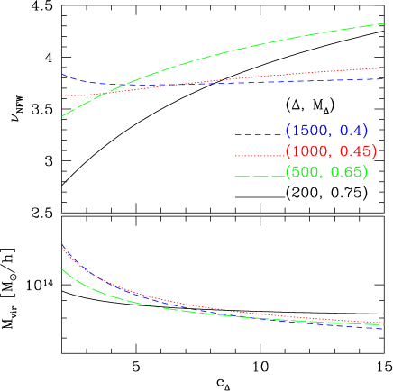
Figure 2: Top: The peak $S/N$ expected for NFW halo as a function of the concentration parameter. Different lines show different spherical overdensity mass shown in unit of $10^{14}h^{-1}M_{\odot}$. The lens and source redshift are set to be 0.3 and 1, respectively. Bottom: Corresponding virial mass is plotted.

The weak lensing peak height for the NFW halo is computed by

$${\cal K}_{\rm NFW}=2\pi\int d\phi~{}\phi~{}\kappa_{\rm NFW}(\phi)U(\phi),$$ (18)

where $\kappa_{\rm NFW}$ is the convergence profile from NFW halo for which we take the smoothly truncated NFW profile (see Oguri & Hamana, 2011; Baltz et al., 2009, for analytic expressions). It is seen from bottom panels of Fig. 1 that the most of the contribution to ${\cal K}_{\rm NFW}$ comes from the matter within the scale radius or from shear data on scales $\theta_{s}<\theta<\theta_{\rm vir}$. We denote the $S/N$ expected from NFW halo by $\nu_{\rm NFW}={\cal K}_{\rm NFW}/\sigma_{\rm shape}$. The expected $S/N$ is shown in Fig. 2 as a function of the concentration parameter. We find that, in the cases of lower $\Delta$, the $S/N$ is sensitive to the concentration parameter (the same argument but for the case of $M_{\rm vir}$ was made by King & Mead (2011)). This can be explained by the fact that the lensing $S/N$ mostly comes from the mass at the inner region of the halo as was shown in Fig. 1. The change in the concentration parameter results in the change in the mass of the inner region, and thus results in the change in the $S/N$. On the other hand, in the cases of higher $\Delta$, the spherical overdensity mass effectively defines the mass of inner region; therefore, the change in the concentration parameter does not affect the $S/N$, though it alters the virial mass. Therefore we can argue that the peak $S/N$ is not a good virial mass indicator but more tightly correlates with the inner mass such as $M_{1000}$. The result appears to be consistent with the finding of Okabe et al. (2010), who argued that weak lensing mass measurement errors are smaller for larger overdensities of $\Delta=500-2000$ than the case for the virial overdensity.

3 Numerical simulations

3.1 Gravitational lensing ray-tracing simulations

We use a large set of ray-tracing simulations that are detailed in Sato et al. (2009) and Oguri & Hamana (2011). It is based on the ray-tracing technique developed in Hamana & Mellier (2001). In what follows we describe only aspects directly relevant to this study.

The ray-tracing simulations are based on $200$ realizations of $N$-body simulations with the box sizes of 240$h^{-1}$ Mpc (particle mass $m_{p}=5.4\times 10^{10}h^{-1}M_{\odot}$). We use the standard multiple lens plane algorithm to simulate gravitational lensing by intervening matter. In this study, we consider a single source redshift of $z_{s}=1$, which is a typical mean source redshift of weak lensing analysis. Note that if redshift information on the source galaxies, e.g. from photometric redshift, is available, one may employ the topographic technique which improves the capability of weak lensing cluster identification (Hennawi & Spergel, 2005; Dietrich & Hartlap, 2010). Instead of using 1000 ray-tracing realizations generated by Sato et al. (2009), we regenerated 200 independent realizations so that the same halo does not appear in different realizations.

Weak lensing mass maps, ${\cal K}$, are generated from lensing shear data by applying the operation eq. (11) on grid points of $2048\times 2048$ with the grid spacing of 0.15 arcmin. We generated two types of mass maps, one is maps without the galaxy shape noise, and the other is maps with the galaxy shape noise. For galaxy shape noise, random ellipticities drawn from the truncated two-dimensional Gaussian (see below) are added to shear data:

$$P(|e|)=\frac{1}{\pi\sigma_{e}^{2}(1-e^{-1/\sigma_{e}^{2}})}\exp\left(-\frac{e^{2}}{\sigma_{e}^{2}}\right),$$ (19)

with $\sigma_{e}=0.4$ and assumed number density of source galaxies of 30 arcmin^-2. Peaks are identified as pixels that have higher values of $\cal K$ than 8 surrounding pixels. Here it should be noted that in the case of the noise added maps, especially for the case of the PEX0 filter, crowds of high peaks caused by the galaxy shape noise tends to form at massive cluster regions. To exclude duplicated detections in each cluster, we apply friends-of-friends (FOF) algorithm with the linking length of 1 arcmin (Maturi et al., 2005), and group together duplicated peaks as a single peak. This procedure generates a catalogue of lensing peaks for each map.

3.2 Dark matter halo catalogue

For each $N$-body output, we identify dark matter haloes using the standard FOF algorithm with the linking parameter of $b=0.2$ and derive a halo mass $M_{\rm FOF}$ for each halo. We define the halo position by the potential minimum of haloes where the gravitational potential is computed from only FOF member particles. In addition to $M_{\rm FOF}$, we compute the spherical overdensity mass with average overdensities of $\Delta=500$ and 1000, which are denoted by $M_{500}$ and $M_{1000}$, respectively.

To evaluate the halo shape, we compute the inertia tensor of the mass distribution:

$$I_{ij} = \int d\mbox{\boldmath$x$}^{3}(x_{i}-\bar{x}_{i})(x_{j}-\bar{x}_{j})\rho(\mbox{\boldmath$x$})$$ (20)

$$= m_{p}\sum_{k=1}^{N_{p}}(x_{i,k}-\bar{x}_{i})(x_{j,k}-\bar{x}_{j}),$$

where $i,j$ run from 1 to 3, $N_{p}$ is the number of FOF member particles of haloes and $\bar{x}_{i}$ denotes the cluster centre defined by the potential minimum. We use the trace of the inertia tensor to estimate the concentration of the halo mass distribution,

$$I\equiv{1\over 3}(I_{11}+I_{22}+I_{33}).$$ (21)

This is compared with the expected value for the uniform overdens sphere:

$$I_{\rm TH}={1\over 5}M_{\rm vir}r_{\rm vir}^{2}.$$ (22)

To evaluate the triaxility of halo shape, we compute the eigenvectors from the inertia tensor and convert them to the axial ratios $a/c$ and $a/b$ ($a\leq b\leq c$). We also compute the angle between the line of sight and the major-axis direction of the halo which we denote as $\theta_{z}$.

Halo catalogues on the light cone are generated by stacking the simulation outputs in the same manner as in the ray-tracing experiments. In summary, each halo in the mock catalogues has data on the mass, redshift, the angular position on the weak lensing mass map and the parameters for the halo shape $I$, $a/c$ and $\theta_{z}$. In addition, for each halo, we compute the NFW-corresponding peak $S/N$ using eq. (18) adopting the mass-concentration relationship eq. (3) for three mass estimates, $M_{\rm FOF}$, $M_{500}$ and $M_{1000}$, which we denote $\nu_{\rm FOF}$, $\nu_{500}$ and $\nu_{1000}$ respectively. Also we compute the virial radius defined by eq. (2), and $I_{\rm TH}$ defined by eq. (22), adopting $M_{\rm FOF}$ as the virial mass.

4 Result

4.1 Halo-peak relationship

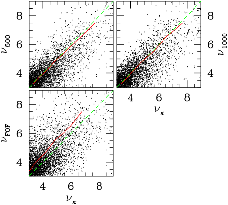
Figure 3: Peak values in the noise-free $\cal K$ map, $\nu_{\kappa}$, is compared with the NFW-corresponding peak $S/N$ computed from $M_{\rm FOF}$ (bottom left), $M_{500}$ (top left) and $M_{1000}$ (top right). The mass maps generated from the Gaussian filter are used. Each point shows the relation for each halo, and the solid line shows the mean of them. Here haloes with $M_{\rm FOF}>1\times 10^{14}h^{-1}M_{\odot}$ at $0.1<z<0.4$ are considered.

We start with matching halo catalogues with weak lensing peaks. To do so, for each halo, the highest peak within the virial radius of the halo (or within 3 arcmin if the virial radius is larger than 3 arcmin) is searched for and is considered as the corresponding peak. We denote the peak heights by $\nu_{\kappa}$.

First we examine the correlation between the $\nu_{\kappa}$ from the noise-free $\cal K$ map and the NFW-corresponding peaks evaluated from the three definitions of the halo mass, $M_{\rm FOF}$, $M_{500}$ and $M_{1000}$. The aim of this analysis is to check the finding in Section 2.2 that the mass definition taking into account only the inner region (such as $M_{1000}$) better correlates with the peak $S/N$ than masses including outer regions (such as $M_{200}$ or $M_{\rm vir}$). Fig. 3 compares $\nu_{\kappa}$ with three NFW-corresponding peaks $\nu_{\rm FOF}$, $\nu_{500}$ and $\nu_{1000}$, where haloes with $M_{\rm FOF}>1\times 10^{14}h^{-1}M_{\odot}$ at $0.1<z<0.4$ are considered. To quantify the correlation, we evaluate the mean and rms scatter of $\delta_{\nu}\equiv(\nu_{\kappa}-\nu_{i})/\nu_{i}$ among peaks with $\nu_{i}>4$, and we find (mean, RMS)$=(-0.11,0.25)$, $(0.017,0.20)$ and $(0.0098,0.19)$ for $i={\rm FOF}$, 500 and 1000, respectively. Thus we find that $\nu_{1000}$ best correlates with $\nu_{\kappa}$, as expected. Based on this result, in what follows, we take $M_{1000}$ as the mass indicator of the haloes. Note that for the NFW halo with $c_{\rm vir}=4$, $M_{1000}/M_{\rm vir}\simeq 0.35$, and $M_{1000}/M_{\rm vir}$ is larger (smaller) for a halo with higher (lower) concentration. We also find that $\nu_{\rm FOF}$-$\nu_{\kappa}$ relationships not only have larger scatters but also show some offset in the mean relationship. One of the reasons may be the mismatch between $M_{\rm FOF}$ computed in $N$-body simulations and $M_{\rm vir}$ defined by overdensity (see also Oguri & Hamana, 2011), presumably caused by the presence of outer substructures that contribute to the FOF mass. In the analysis above, the mass maps generated from the Gaussian filter are used though the results are found not to be affected by choice of the filter.

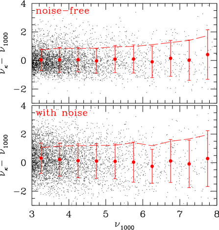
Figure 4: Relationship between $\nu_{1000}$ and $\nu_{\kappa}$ as a function of $\nu_{1000}$. The dots show the relation for each halo and the filled circles with error bars show the mean and the rms scatter, and the dashed curve show the value of the rms scatter. The $\cal K$ maps generated from the Gaussian filter are used, and only the haloes with $M_{1000}>3\times 10^{13}h^{-1}M_{\odot}$ at $0.1<z<0.4$ are considered. The top and bottom panels show results without and with the shape noise, respectively.

Next we examine the influence of the following three effects on the peak $S/N$; (1) the galaxy shape noise, i.e., the noise due to the intrinsic shapes of source galaxies used for weak lensing analysis, (2) the projection of structures along the line of sight of clusters, which we call the cosmic noise, and (3) the diversity of dark matter distributions of haloes, which we call the halo shape effect. To do so, the mass maps generated from the Gaussian filter are used though the results are found not to be strongly dependent on the choice of the filter. With our choice of parameters for the galaxy shape noise (e.g., $\sigma_{e}=0.4$ and $n_{g}=30$ arcmin^-2), the rms of the galaxy shape noise is $\sigma_{\rm shape}=0.02$, which should act as the additive noise in $\nu_{\kappa}$. The analytic way to estimate the cosmic noise was developed by Hoekstra (2001) under the assumption that the halo and the large-scale structures are uncorrelated, and for the cosmological model adopted in this paper and the Gaussian window function, its rms is estimated to be $\sigma_{\rm cosmic}=0.01$, which should again act as the additive noise. The halo shape effect should, in a crude approximation, act as the multiplicative noise in the peak $S/N$. We estimate its amplitude using the ray-tracing simulation data. We evaluate scatters in $\nu_{\kappa}-\nu_{1000}$ relations as a function of $\nu_{1000}$, and results are plotted in Fig. 4.

The result for the noise-free $\cal K$ map case shown in the top panel of Fig. 4 indicates that the rms increase with $\nu_{1000}$. Since only the cosmic noise and halo shape effect are playing in this shape noise free case, and the cosmic noise should be independent of the $S/N$, the dependence of the rms on $\nu_{1000}$ is most likely originated from the halo shape effect. We estimate from the rms measured from $\nu_{\kappa}-\nu_{1000}$ relationship and the expectation value of $\sigma_{\rm cosmic}=0.01$ (thus $\sigma_{\rm cosmic}/\sigma_{\rm shape}=0.5$) that the rms of the halo shape effect scales approximately $\sigma_{\rm halo}\sim(0.1-0.2)\times{\cal K}_{NFW}$ (i.e., $\sigma_{\rm halo}/\sigma_{\rm shape}\sim(0.1-0.2)\times\nu$). Thus for very massive haloes the halo shape effects can be larger than the other noises (the qualitatively same argument was made by Tan & Fan (2005)). However, it should be noted that for a very shallow survey the above argument may not be the case as $\sigma_{\rm shape}$ scales with the source galaxy number density as $\sigma_{\rm shape}\propto n_{g}^{-0.5}$. In the noise added case plotted in the bottom panel of Fig. 4, the mean value is slightly greater than zero, quantitatively $\langle\nu_{\kappa}-\nu_{1000}\rangle\sim 0.25$ thus $\sim 5$ per cent for the $\nu=5$ peak. This is because we consider the peaks that are affected by the shape noise in an asymmetric way as discussed in Hamana, Takada, & Yoshida (2004).

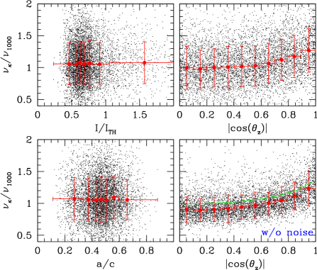
Figure 5: Relationship between $\nu_{1000}$ and $\nu_{\kappa}$ as a function of $I/I_{\rm TH}$ (top left), $a/c$ (bottom left) and $|\cos(\theta_{z})|$ (right panels). Here haloes with $M_{1000}>3\times 10^{13}h^{-1}M_{\odot}$ at $0.1<z<0.4$ are considered. The dots show the relationship for each halo and filled circles show mean, vertical error bars show the rms scatter, and the horizontal error bars show the range where sample is taken. The $\cal K$ maps with the shape noise generated from the Gaussian filter are used except for the bottom-right panel where the noise-free $\cal K$ maps are used. The green curve in the bottom-right panel shows the theoretical prediction based on the triaxial halo model.

We now discuss details of the halo shape effect. In Fig. 5, the fractional difference between $\nu_{1000}$ and $\nu_{\kappa}$ measured from $\cal K$ map (with the galaxy shape noise added) is shown as a function of the halo concentration $I/I_{\rm TH}$ (top-left panel), the axis ratio $a/c$ (bottom-left panel) and the halo orientation with respect to the line-of-sight direction $|\cos(\theta_{z})|$ (right panels). Dots indicate values for each halo, where we consider haloes with $M_{1000}>3\times 10^{13}h^{-1}M_{\odot}$ at $0.1<z<0.4$ with the mean $S/N$ of this halo sample being $\langle\nu_{1000}\rangle=3.7$. Filled circles show average values. We find that there exists (1) a clear correlation between the halo orientation and the peak height deviations from the NFW model prediction, whereas (2) no correlation for the halo shape parameters ($I/I_{\rm TH}$ and $a/c$). The results indicate that the intrinsic halo shape (concentration and axis ratio) does not cause a systematic bias in the peak heights as long as one employs an appropriate definition of the halo mass such as $M_{1000}$, but just contribute to the scatter. However the halo orientation does cause the systematic bias because the line-of-sight projected mass at the inner region depends strongly on the halo orientation (see also Oguri et al., 2005; Gavazzi, 2005). In the bottom-right panel of Fig. 5, the theoretical prediction based on the triaxial halo model (Jing & Suto, 2002; Oguri & Blandford, 2009) is also shown (see Section 2.1). We find that the triaxial model nicely reproduces the orientation dependence of the peak heights found in ray-tracing simulations, except for the small offset which is originated from an approximation involved in the triaxial haloes (see Oguri et al., 2005).

4.2 Selection bias in weak lensing selected clusters

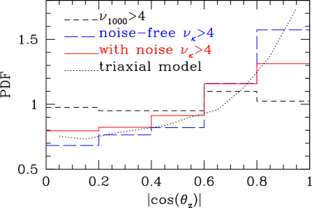
Figure 6: Probability distribution functions of the halo orientation with respect to the line-of-sight direction, $|\cos(\theta_{z})|$, for weak lensing selected clusters. We adopt the peak height threshold value of $\nu=4$. The dashed histogram is for the NFW-corresponding peaks, i.e., peak heights evaluated by the spherical NFW model via spherical overdensity masses, the long-dashed histogram for the peak heights measured from the noise-free $\cal K$ map, and the solid histogram for the peak heights measured from the noise added $\cal K$ map. The dotted curve shows the analytic model expectation based on the triaxial halo model.

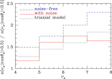
Figure 7: The halo orientation bias as a function of the peak $S/N$ threshold. We quantify the bias by the ratio of the numbers of haloes with the major axis aligned to the line-of-sight direction ($|\cos\theta_{z}|>0.5$) to those with anti-aligned ($|\cos\theta_{z}|<0.5$). The dashed histogram is for the peak heights measured from the noise-free $\cal K$ map, and the solid histogram for the peak heights measured from the noise added $\cal K$ map. The dotted histogram shows the analytic model prediction based on the triaxial halo model.

Given the strong dependence of the peak heights on the halo orientation, we shall now investigate its impact on weak lensing selected cluster catalogues. In Fig. 6, we show the probability distribution function (PDF) of the halo orientation with respect to the line-of-sight direction, $|\cos(\theta_{z})|$, for haloes with peak heights above the threshold value $\nu=4$. Here we include only haloes at $0.1<z<0.4$ for simplicity. Different histograms are for different causes; NFW-corresponding peaks (dashed), peak heights measured from the noise-free $\cal K$ map (long-dashed), and the noise added map (solid). In addition, the same PDF computed with analytic triaxial halo model (see Section 2.1) is also plotted by the dotted line, which should be compared with the noise-free case because the galaxy shape noise is not added in the triaxial model calculation. The PDF for the NFW-corresponding peaks ($\nu_{1000}$) is flat. This is exactly expected because the NFW-corresponding peak heights are computed from $M_{1000}$ assuming the spherical NFW profile, and hence they should not depend on the orientations of haloes. On the other hand, the PDFs for the measured peaks are significantly skewed such that the major axes of haloes are preferentially aligned with the line-of-sight direction. To quantify the bias, we introduce an estimator defined by the ratio between the numbers of haloes with the major axis aligned to the line-of-sight direction ($|\cos\theta_{z}|>0.5$) and anti-aligned ($|\cos\theta_{z}|<0.5$), i.e., $b_{z}\equiv n(|\cos\theta_{z}|>0.5)/n(|\cos\theta_{z}|<0.5)$. For the cases shown in Fig. 6, the bias are $b_{z}=1.7$ and 1.4 for the noise-free and noise added cases, respectively. For the case of the NFW-corresponding peaks we have $b_{z}=1.07$, suggesting that the error in the above estimation is less than 10 per cent.

In addition, we examine the bias as a function of the peak heights using the estimator, $b_{z}(\nu_{\kappa})\equiv n(\nu_{\kappa};|\cos\theta_{z}|>0.5)/n(\nu_{\kappa};|\cos\theta_{z}|<0.5)$. The results are shown in Fig.  7. While the statistic is not very good especially for higher $S/N$ bins because of a limited number of peaks, one can clearly see a trend that the orientation bias is larger for higher $S/N$. This is presumably because the halo shape effect is multiplicative to the $S/N$. Although the results are not accurate enough to make precise predictions, we find that the bias is $\sim 1.5$ for high $S/N$ peaks of $\nu_{\kappa}\ga 5$. and $\sim 1.2$ for $\nu_{\kappa}\sim 4$. Therefore the orientation bias is one of the most significant selection bias in weak lensing selected cluster catalogues. Its impact on cluster related sciences should be taken into consideration. The results shown in Figs. 5, 6, and 7 indicates that the analytic triaxial model predictions are in very good agreement with the trends found in ray-tracing simulations. This confirms that the orientation bias comes from the intrinsic triaxial shapes of haloes, rather than the effect of surrounding matter around clusters, because such correlated matter is not included in our analytic triaxial model calculations.

We note that the strong halo orientation bias was also found in previous strong lensing studies as well. Hennawi et al. (2007) used a large set of ray-tracing simulations to show that major axes of clusters producing giant arcs are preferentially aligned with the line-of-sight direction, with the level of the bias similar to what found in this paper. Oguri & Blandford (2009) reported that clusters having larger Einstein radii have larger orientation bias, based on the triaixl halo model. Similar result for strong lensing clusters was obtained also by Meneghetti et al. (2010). Our result indicates that similar orientation bias exists for weak lensing selected clusters as well.

4.3 Completeness

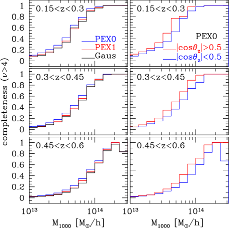
Figure 8: Completeness as a function of the halo mass. From top to bottom panels, we change the redshift range from lower to higher mean redshifts. Left panels: Different histograms show results for different filters. Blue, red, and black histograms are for the PEX0, PSX1 and Gaussian filters, respectively. Right panels: The red histogram is for the the haloes with $|\cos(\theta_{z})|>0.5$, i.e., haloes with major axes aligned with the line-of-sight direction, whereas the blue histogram is for anti-aligned haloes.

To see the impact of the halo orientation bias, we examine the completeness which we define by the fraction of haloes identified as high peaks above a given threshold ($\nu_{min}$) in the $\cal K$ map relative to all the haloes, namely, $n(M,z;\nu_{\kappa}>\nu_{min})/n(M,z)$. The choice of the threshold is arbitrary, usually it is chosen considering the trade-off between the sample size and the fraction of the false positives (see Section 4.4). Here we adopt $\nu_{min}=4$. The completeness for different filters are shown in left panels of Fig. 8. We find that the PEX0 filter is the best in terms of the completeness, although the difference between filters is small, 10 per cent at most. Right panels of Fig. 8 compares the completeness for haloes with $|\cos\theta_{z}|>0.5$ (red histogram) with the others (blue), where the $\cal K$ maps with PEX0 filter are used. We find that the effect of the halo orientation bias is visible for the intermediate mass haloes for which $\nu_{\rm NFW}\sim\nu_{\rm min}$. The reason is that for the very massive/small haloes, the $S/N$ differs very much from $\nu_{\rm min}$, meaning that the spread of $\nu$ produced by the halo shape effect does not affect the detectability of those haloes. Thus the completeness of haloes with $\nu_{\rm NFW}\sim\nu_{min}$ are mostly affected by the halo orientation bias. The difference of the amplitude for the completeness is about 20 per cent for those haloes.

4.4 Peak counts and purity

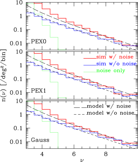
Figure 9: Number counts of weak lensing peaks for three filters from top to bottom panels. The red and blue histograms are measurements from ray-tracing simulations with and without galaxy shape noise, respectively. The green histogram is the number count of peaks from the pure noise map. The long-dashed and dashed curves are analytical predictions using the spherical NFW profile, with and without shape noise taken into account, respectively.

Table 1: Summary of the number density (per 1 deg²) of weak lensing mass peaks (in noise added $\cal K$ maps) above thresholds.

filter	$N_{\rm peak}(\nu_{\kappa}>4)$	$N_{\rm peak}(\nu_{\kappa}>5)$	$N_{\rm peak}(\nu_{\kappa}>6)$
PEX0	3.3	0.70	0.22
PEX1	2.7	0.59	0.19
Gauss	2.2	0.53	0.19

So far we discussed connections between the weak lensing properties of clusters and dark matter halo properties. Here, we study the subject from a different viewpoint, i.e., we examine properties of the weak lensing peak sample in terms of peak counts and purity, paying special attention to the comparison among three filters.

First we examine peak counts and compare with the analytic model. In Fig. 9, peak counts measured from three $\cal K$ maps (the galaxy noise free, noise added, and the pure noise cases) are presented for three filters. The number densities of peaks (in noise added $\cal K$ maps) above the given thresholds are summarized in Table 1. We find that the PEX0 filter yields the largest peak counts, specifically about 20 per cent larger than the PEX1 filter, and even larger difference from the Gaussian filter. This is a natural consequence that the PEX0 filter mimics the optimal filter developed by Maturi et al. (2005) which is designed for maximizing the $S/N$ of $\cal K$ from the NFW halo (see Pace et al. (2007) for the test of the capability of the optimal filter against numerical simulations). To compute the analytic prediction of the peak counts, we follows the so-called halo model first developed by Kruse & Schneider (2000) (see also Bartelmann, King & Schneider, 2001; Hamana, Takada, & Yoshida, 2004), in which it is assumed that high peaks are dominated by lensing signals from single massive haloes. Here we adopt the spherical NFW density profile for the analytic calculation of the number count, because we include the effect of the halo triaxiality via the halo shape noise as described below. To take into account the effect of noise, we employ the approximate approach developed by Hamana, Takada, & Yoshida (2004) with some modification. Specifically, we make the following three assumptions. (1) Very high peaks are neither removed nor generated by the noise but their peak heights are altered by the noise. (2) The scatter in peak heights with respect to the corresponding NFW peak height follows the Gaussian distribution with the standard deviation of $\sigma_{\rm peak}$. While in Hamana, Takada, & Yoshida (2004) only the galaxy shape noise was taken into accounted, here we include both the cosmic noise and halo shape noise, in addition to the galaxy shape noise. (3) Within a small range of the peak height ($\nu$), the peak counts can be approximated by the exponential form $n_{\rm peak}(\nu)=n_{\ast}\exp(p\nu)$, with a constant exponential index of $p$. Under these assumptions the peak counts in the presence of the noises are given by (Hamana, Takada, & Yoshida, 2004),

$$n_{\rm noisy}(\nu)\simeq\exp\left({{f^{2}p^{2}}\over{2}}\right)n_{\rm peak}(\nu),$$ (23)

where $f=\sigma_{\rm peak}/\sigma_{\rm noise}$. To estimate $f$, we assume the proportion of $\sigma_{\rm shape}:\sigma_{\rm cosmic}:\sigma_{\rm halo}=2:1:1$. For the case of the Gaussian filter, this corresponds to $\sigma_{\rm halo}=0.01$ which is a reasonable approximation for peaks with $\nu\sim 5$ (see Section 4.1). We take the quadrature sum of these three components to obtain $f\simeq 1.2$. The peak counts computed in this method are presented in Fig. 9. We find that for high $S/N$ of $\nu\ga 5$ the improved analytic prediction agrees well with the measurements, whereas for lower $S/N$ the measured counts are slightly larger than the prediction. A possible origin of the excess is the false signals which we examine below.

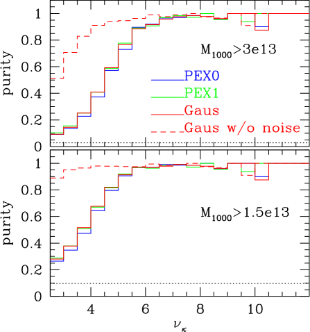
Figure 10: The purity for the three filters are plotted by lines in different colors. The dashed histogram is for the noise-free case. Top panel is for the case where peaks are matched with haloes with $M_{1000}>3\times 10^{13}h^{-1}M_{\odot}$, whereas bottom panel is for $M_{1000}>1.5\times 10^{13}h^{-1}M_{\odot}$. The horizontal dotted line shows the probability that a peak is matched with a randomly distributed halo by chance.

Finally, we examine the purity which we here define by the fraction of peaks which are associated with true haloes among all the peaks. However, in practice, the purity is not uniquely defined quantity because of the following two ambiguities. One is the allowed separation between peak position and halo position. The other is the minimum mass of haloes allowed to be associated with peaks. We adopt the minimum halo mass of $M_{1000}=3\times 10^{13}h^{-1}M_{\odot}$ or $1.5\times 10^{13}h^{-1}M_{\odot}$ based on the detectability study shown in Fig. 8. Considering the virial radii of those haloes, we fix the maximum separation at 3 arcmin. The results are presented in Fig. 10. We also plot the probability that a peak matched with a randomly distributed halo (with the same number density as the true halo catalogue) by chance by the horizontal dotted line, which gives an estimate of the chance coincidence between peaks and unrelated haloes. We find that the probability of the chance matching is not significant for our choice of the minimum masses and the allowed separation. The purity is not dependent on the choice of the filter, and is very high (i.e., the false positive rate is very small) for peaks with $\nu>6$. However the purity drops rapidly at lower $S/N$, and it becomes about 50 per cent at $\nu\sim 4$. We argue that this accounts for the excess in the peak counts over the theoretical prediction found in Fig. 9. In the same figure, we also plot the purity measured from the galaxy shape noise free case. The false positives in this case may arise from chance projections such as the line-of-sight projection of small multiple haloes or filamentary structure. As the purity for the noise-free case is found to be greater than 90 per cent for $\nu>4$, we conclude that the contamination of such chance projection is not significant.

5 Comparison with observations

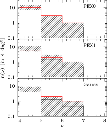
Figure 11: Red histogram shows the number count of peaks measured from real weak lensing $\cal K$ maps generated from 4 deg² of Suprime-Cam data (see Appendix A for details). Results from mock simulation of 4 deg² survey are shown by black histogram (the average among 200 realizations) with shading (the range enclosing 68 per cent). Note that on the highest bin, peak counts are zero in most of the realizations and non-zero counts are measured in a small fraction of realizations, therefore the average is non-zero but the 68 per cent enclosing region is not defined.

It is worth checking the results of our mock simulation data against real observational results. In Fig. 11, we compare the peak counts measured from real weak lensing $\cal K$ maps generated from 4 deg² of Subaru/Suprime-Cam data with results from the mock simulations. A description of the Suprime-Cam data and data analysis is given in Appendix A. In short, the Suprime-Cam data consist of four fields with fairly uniform data quality (with respect to the depth and seeing condition) with the number density of galaxies used for weak lensing analysis is $n_{g}\simeq 27$ arcmin^-2 and the rms ellipticity of $\sigma_{\rm shape}=0.4$ which are in a good agreement with the values adopted in the mock simulations. The mean source redshift is not known as there is no large spectroscopic/photometric redshift galaxy catalogue reaching the depth of the data ($i^{\prime}\sim 25.5$ AB mag), but the value of $\langle z_{s}\rangle=1$ assumed in mock simulations is reasonable (see also Oguri et al., 2012). We generated $\cal K$ maps with the three filters under consideration, and we searched for peaks in the $\cal K$ maps. The peaks located within 1 arcmin from the field boundary were discarded as the regions are likely affected by the partial lack of data. The total area used for peak finding is 4 deg². We detect 14, 9 and 7 peaks with $\nu>4$ for the PEX0, PEX1 and Gaussian filter, respectively. To measure the peak counts from mock simulations under a similar survey condition, we extracted a contiguous 4 deg² region from each mock weak lensing realization, and measured peak counts. We computed the average counts and the range enclosing 68 per cent of 200 realizations and show in Fig. 11. We find that (i) peak counts from real data are in a reasonable agreement with the expectation from mock data, and (ii) its dependence on the filter is similar to that expected from the mock data. Of course this comparison tests only a limited aspect of the mock simulation, yet the agreements can be regarded as a piece of evidence that our numerical simulations based on the standard cosmological model and realistic noise parameters produce reasonably realistic mock data.

6 Summary and discussions

We have investigated scatter and bias in weak lensing selected clusters, employing both the analytic model description of dark matter haloes and the numerical mock data of weak lensing cluster surveys generated with gravitational lensing ray-tracing through a large set of $N$-body simulations. We have paid special attention to the effects of diversity in the dark matter distribution of haloes. Our major findings are summarized as follows.

1. We have examined the relationship between the peaks measured from the noise-free $\cal K$ map and the expected peak values computed assuming the spherical NFW profile with three cluster mass definitions, $M_{\rm FOF}$, $M_{500}$ and $M_{1000}$. We have found that the expected peak value computed with $M_{1000}$ best correlates with the measured peak heights. This confirms the finding in Section 2.2 that the lensing $S/N$ computed with the spherical overdensity mass with higher mean interior density is less affected by variation in halo concentrations than those with lower interior density. An implication to observational studies is that the peak $S/N$ is not a good virial mass indicator but is more tightly related to the inner mass such as $M_{1000}$.

2. We have examined the influence of the diversity of the halo shape on the peak $S/N$ values by comparing the peaks measured from the noise-free $\cal K$ map with the NFW-corresponding peak heights computed with $M_{1000}$ using the spherical NFW profile. We have found that the rms of the halo shape effect scales approximately $\sigma_{\rm halo}\sim(0.1-0.2)\times{\cal K}_{NFW}$ (i.e., $\sigma_{\rm halo}/\sigma_{\rm shape}\sim(0.1-0.2)\times\nu$). We therefore conclude that the scatter caused by the halo shape effect can be larger than the ones from other noises for very massive haloes.

3. We have found a clear correlation between the halo orientation and the peak heights, such that haloes whose major axes are aligned with the line-of-sight direction tend to generate a higher peak than the expectation of the spherical NFW model. Using both numerical and analytic approaches, we have examined the systematic bias caused by the orientation effect. We have evaluated the bias using the ratio $b_{z}$ between the numbers of haloes (identified with peak $S/N$ above certain thresholds) with the major axis aligned with the line-of-sight direction ($|\cos\theta_{z}|>0.5$) and those anti-aligned. We found that the bias is $b_{z}=1.4$ for the threshold of $\nu_{min}=4$, indicating that orientation bias is quite strong. In addition, we have found that the bias is larger for higher $S/N$ peaks, because the halo shape effect is multiplicative to $S/N$. Thus the orientation bias is a non-negligible selection bias in weak lensing selected cluster catalogues. We have also examined the effect of the halo orientation bias on the completeness and found that the haloes with $\nu_{\rm NFW}\sim\nu_{min}$ are most affected by the halo orientation bias, and its amplitude for the completeness is found to be about 20 per cent for those haloes. We have shown that the analytic triaxial halo model explains the orientation bias found in ray-tracing simulations very well, which confirms that the halo triaxiality is the main cause of the orientation bias.

4. We have compared the capability of three filters with respect to the the completeness, peak counts and purity. We have found that the PEX0 works best, which gives about 10 per cent better completeness for haloes with $\nu\sim\nu_{min}$ than the other two filters and about $\ga 20$ per cent larger peak counts with the similar level of purity.

5. We have developed a prescription to analytically compute the number count of weak lensing peaks which improve earlier works (Kruse & Schneider, 2000; Bartelmann, King & Schneider, 2001; Hamana, Takada, & Yoshida, 2004). Specifically, we have employed an approximate way to include the scatters in peak heights caused by all the three sources addressed in this paper; the galaxy shape noise, the cosmic noise, and the halo shape noise. We have tested the improved model against the mock ray-tracing simulation data, and found that the analytic predictions agree well with the simulation results for a high $S/N$ of $\nu\ga 5$.

6. We have compared the number counts of peaks from the numerical mock data with those from 4 deg² of real Subaru/Suprime-cam data. Although the comparison is limited by small number statistics, we have found that both the number counts and their smoothing filter dependence are in reasonable agreement between the mock data and the observation.

Appendix A Weak lensing analysis of Suprime-Cam data

We collected $i^{\prime}$-band data taken with the Subaru/Suprime-Cam (Miyazaki et al., 2002) from the data archive SMOKA, under the following three conditions: data are contiguous with at least four pointings, the exposure time for each pointing is longer than 1800 sec, and the seeing full width at half-maximum (FWHM) is better than 0.65 arcsec. Four data sets meet these requirements and are summarized in Table 2.

Table 2: Summary of data sets. See Figs. 12-15 for the coordinate of each field

field name	areaa	$T_{exp}$b	seeingc	$n_{g}$d
SXDS	0.99 (0.77)	6000	0.52	27.6
COSMOS	1.85 (1.32)	2400	0.53	26.5
Lockman-hole	0.74 (0.56)	3600	0.51	27.3
ELAIS N1	1.99 (1.39)	3600	0.57	26.6

^a Area after masking regions affected by bright stars in unit of deg². The numbers in parentheses are the area after cutting the edge regions within 1 arcmin from the boundary.
^b Exposure time for each pointing in the unit of seconds.
^c Median of seeing full width at half-maximum in the unit of arcsec.
^d Number density of galaxies used for the weak lensing analysis in the unit of arcmin^-2.

Each CCD data was reduced using the SDFred software (Yagi et al, 2002; Ouchi et al, 2004). Note that we conservatively use the data only within 15 arcmin radius from the field centre of Suprime-Cam, because at the outside of that, the point spread function (PSF) becomes elongated significantly which may make the correction for the PSF inaccurate. Then mosaic stacking was done with SCAMP (Bertin, 2006) and SWarp (Bertin et al, 2002). Object detections were performed with SExtractor (Bertin & Arnouts, 1996) and hfindpeaks of IMCAT software (Kaiser, Squires & Broadhurst, 1995), and two catalogues were merged by matching positions with a tolerance of 1 arcsec.

For weak lensing measurements, we follow the so-called KSB method described in Kaiser, Squires & Broadhurst (1995), Luppino & Kaiser (1997), and Hoekstra et al. (1998). Stars are selected in a standard way by identifying the appropriate branch in the magnitude half-light radius ($r_{h}$) plane, along with the detection significance cut $S/N>10$. The number density of stars is found to be $\sim 1$ arcmin^-2 for the four fields. We only use galaxies met the following three conditions, (i) the detection significance of $S/N>3$ and $nu>10$ where $nu$ is an estimate of the peak significance given by $hfindpeaks$, (ii) $r_{h}$ is larger than the stellar branch, and (iii) the AB magnitude is in the range of $22<i^{\prime}<25.5$ (where MAG_AUTO given by the SExtractor is used for the magnitude). The number density of resulting galaxy catalogue is quite uniform not only over each field but also among four fields (see Table 2). We measure the shapes of objects by getshapes of IMCAT, and correct for the PSF by the KSB method. The rms of the galaxy ellipticities after the PSF correction is found to be 0.4 for all the four fields.

Table 3: Summary of high peaks.

field-ID	R.A.	Dec.	$\nu$ (Peak-$S/N$)
	[deg]	[deg]	PEX0	PEX1	GAUSS
SXDS-1	34.0185	$-5.0755$	4.1	3.8	3.6
COSMOS-1	150.5067	2.7657	5.2	5.2	5.1
COSMOS-2	150.2063	1.8283	4.3	4.4	4.4
COSMOS-3	150.1838	1.6583	4.0	3.9	3.7
COSMOS-4	150.0987	2.7158	4.0	3.7	2.9
COSMOS-5	149.8486	2.2883	5.1	4.9	4.3
ELAIS-1	243.3380	55.4445	4.0	4.0	3.8
ELAIS-2	242.8025	55.5614	6.5	6.5	6.6
ELAIS-3	242.6855	55.4296	4.2	4.2	3.6
ELAIS-4	241.2850	55.6263	4.2	4.2	4.2
ELAIS-5	241.2278	54.5485	4.2	3.9	3.4
ELAIS-6	241.2034	54.4808	4.1	3.9	3.4
ELAIS-7	241.1764	54.5356	5.3	5.2	5.2
ELAIS-8	240.8272	55.1126	4.3	4.3	4.3

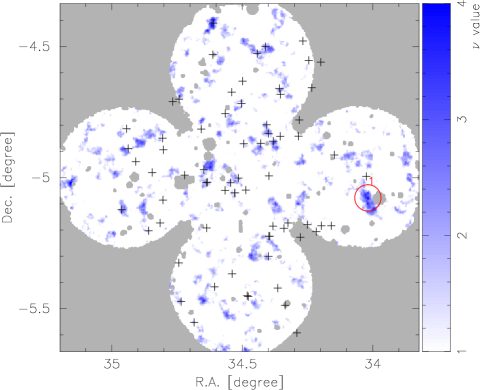
Figure 12: $\cal K$ maps for the SXDS field, generated with the PEX0 filter are plotted by blue scale. Gray regions are either the region outside the analyzed area (within 15 arcmin from the field centre of Suprime-Cam) or masked regions where the data are affected by bright stars. High peaks with $\nu>4$ are marked with red circle along with ID given in Table  3. The Plus symbols show positions of known clusters taken from a compilation by NASA/IPAC Extragalactic Database (NED).

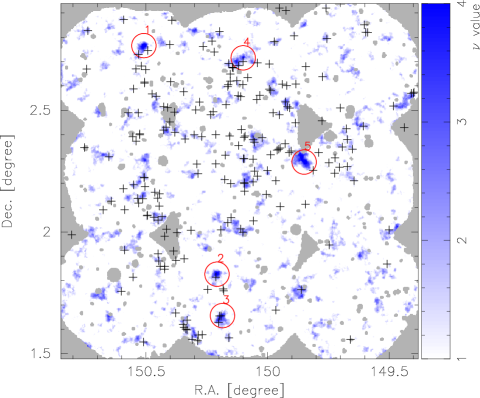
Figure 13: Same as Fig. 12 but for the COSMOS field.

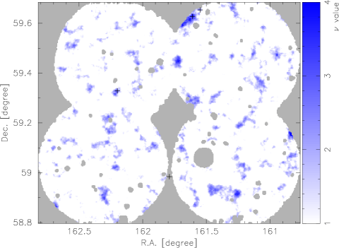
Figure 14: Same as Fig. 12 but for the Lockman-hole field.

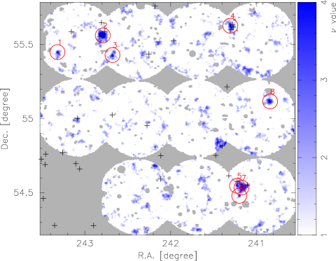
Figure 15: Same as Fig. 12 but for the ELAIS N1 field.

Weak lensing $\cal K$ are computed from galaxy ellipticity (after the PSF correction) data with three filters under consideration on regular grid points with a grid spacing of 0.15 arcmin. We then identify high peaks from the $\cal K$ maps. Peaks located within 1 arcmin from the field boundary were discarded because such regions are likely affected by the partial lack of data. The total area used for the peak finding is 4 deg². We detect 14, 9 and 7 peaks with $\nu>4$ for the PEX0, PEX1 and Gaussian filter, respectively. High peaks with $\nu>4$ are summarized in Table 3, and peak counts are plotted in Fig. 11, in which a good agreement with mock simulation data is found. In Figs. 12-15, $\cal K$ maps generated with the PEX0 filter are shown in which high peaks are marked with circles. We also mark known clusters taken from a compilation by NASA/IPAC Extragalactic Database (NED) by the plus symbols. It is seen that many but not all high peaks are associated with known clusters. It should be noted that the known cluster sample plotted in the figures is just a compilation of many individual cluster catalogues identified by many different techniques, and thus is not homogeneous even over a single field.

References

- Baltz et al. (2009) Baltz E. A., Marshall P., Oguri M., 2009, JCAP, 1, 15
- Bartelmann, King & Schneider (2001) Bartelmann M., King, L. J., Schneider P., 2001, A&A, 378, 361
- Bellagamba et al. (2011) Bellagamba F., Maturi M., Hamana T., Meneghetti M., Miyazaki S., Moscardini L., 2011, MNRAS, 413, 1145
- Bertin & Arnouts (1996) Bertin E., Arnouts S., 1996, A&AS, 317, 393
- Bertin et al (2002) Bertin E., Mellier Y., Radovich M., Missonnier G., Didelon P., Morin B., 2002, ASP Conference Proceedings, 281, 228
- Bertin (2006) Bertin E., 2006, ASP Conference Series, 351, 122
- Böhringer et al. (2004) Böhringer H., et al., 2004, A&A, 425, 367
- Broadhurst et al. (2008) Broadhurst T., Umetsu K., Medezinski E., Oguri M., Rephaeli Y., 2008, ApJ, 685, L9
- Bullock et al. (2001) Bullock J. S., Kolatt T. S., Sigad Y., Somerville R. S., Kravtsov A. V., Klypin A. A., Primack J. R., Dekel A., MNRAS, 2001, 321, 559
- Clowe, De Lucia, & King (2004) Clowe D., De Lucia G., King L., 2004, MNRAS, 350, 1038
- Corless & King (2009) Corless V. L., King L. J., 2009, MNRAS, 396, 315
- Dahle (2006) Dahle H., 2006, ApJ, 653, 954
- Dietrich et al. (2012) Dietrich J. P., Böhnert A., Lombardi M., Hilbert S., Hartlap J., 2012, MNRAS, 419, 3547
- Dietrich & Hartlap (2010) Dietrich J. P., Hartlap J., 2010, MNRAS, 402, 1049
- Duffy et al. (2008) Duffy A. R., Schaye J., Kay S. T., Dalla Vecchia C., 2008, MNRAS, 390, L64
- Fan, Shan & Liu (2010) Fan Z., Shan H., Liu J., ApJ, 719, 1408
- Feroz & Hobson (2012) Feroz F., Hobson M. P., 2012, MNRAS, 420, 596
- Gavazzi (2005) Gavazzi R., 2005, A&A, 443, 793
- Gavazzi & Soucail (2007) Gavazzi R., Soucail G., 2007, A&A, 462, 459
- Hamana & Mellier (2001) Hamana T., Mellier Y., 2001, MNRAS, 327, 169
- Hamana & Miyazaki (2008) Hamana T., Miyazaki S., 2008, PASJ, 60, 1363
- Hamana, Takada, & Yoshida (2004) Hamana T., Takada M., Yoshida N., 2004, MNRAS, 350, 893
- Hennawi & Spergel (2005) Hennawi J. F., Spergel D. N., 2005, ApJ, 624, 59
- Hennawi et al. (2007) Hennawi J. F., Dalal N., Bode P., Ostriker J. P., 2007, ApJ, 654, 714
- Hoekstra et al. (1998) Hoekstra H., Franx M., Kuijken K., Squires G., 1998, ApJ, 504, 636
- Hoekstra (2001) Hoekstra H., 2001, A&A, 370, 743
- Jing & Suto (2002) Jing Y. P., Suto Y., 2002, ApJ, 574, 538
- Kaiser, Squires & Broadhurst (1995) Kaiser N., Squires G., Broadhurst T., 1995, 449, 460
- King & Mead (2011) King L. J., Mead J. M. G., 2011, MNRAS, 416, 2539
- Kubo et al. (2009) Kubo J. M., Khiabanian H., Dell’Antonio I. P., Wittman D., Tyson J. A., 2009, ApJ, 702, 980
- Kurtz et al. (2012) Kurtz M. J., Geller M. J., Utsumi Y., Miyazaki S., Dell’Antonio I. P., Fabricant D. G., 2012, ApJ, 750, 168
- Kruse & Schneider (2000) Kruse G., Schneider P., 2000, MNRAS,318, 321
- Luppino & Kaiser (1997) Luppino G. A., Kaiser N., 1997, ApJ, 475, 20
- Macciò, Dutton, & van den Bosch (2008) Macciò A. V., Dutton A. A., van den Bosch F. C., 2008, MNRAS, 391, 1940
- Mahdavi et al. (2008) Mahdavi A., Hoekstra H., Babul A., Henry J. P., 2008, MNRAS, 384, 1567
- Mantz et al. (2010) Mantz A., Allen S. W., Rapetti D., Ebeling H., 2010, MNRAS, 406, 1759
- Marian, Smith, & Bernstein (2010) Marian L., Smith R. E., Bernstein G. M., 2010, ApJ, 709, 286
- Marriage et al (2011) Marriage T. A., et al 2011, ApJ, 737, 61
- Maturi et al. (2005) Maturi M., Meneghetti M., Bartelmann M., Dolag K., Moscardini L., 2005, A&A, 442, 851
- Medezinski et al. (2010) Medezinski E., Broadhurst T., Umetsu K., Oguri M., Rephaeli Y., Benítez N., 2010, MNRAS, 405, 257
- Meneghetti et al. (2010) Meneghetti M., Fedeli C., Pace F., Gottlöber S., Yepes G., 2010, A&A, 519, A90
- Miyazaki et al. (2002) Miyazaki S., et al., 2002, ApJ, 580, L97
- Miyazaki et al. (2002) Miyazaki S., et al., 2002, PASJ, 54, 833
- Miyazaki et al. (2007) Miyazaki S., Hamana T., Ellis R. S., Kashikawa N., Massey R. J., Taylor J., Refregier A., 2007, ApJ, 669, 714
- Nakamura & Suto (1997) Nakamura T. T., Suto Y., 1997, PThPh, 97, 49
- Navarro, Frenk, & White (1997) Navarro J. F., Frenk C. S., White S. D. M., 1997, ApJ, 490, 493
- Oguri & Keeton (2004) Oguri M., Keeton C. R., 2004, ApJ, 610, 663
- Oguri, Lee, & Suto (2003) Oguri M., Lee J., Suto Y., 2003, ApJ, 599, 7
- Oguri & Hamana (2011) Oguri M., Hamana T. 2011, MNRAS, 414, 1851
- Oguri et al. (2005) Oguri M., Takada M., Umetsu K., Broadhurst T., 2005, ApJ, 632, 841
- Oguri et al. (2009) Oguri M., et al., 2009, ApJ, 699, 1038
- Oguri & Blandford (2009) Oguri M., Blandford R. D., 2009, MNRAS, 392, 930
- Oguri et al. (2010) Oguri M., Takada M., Okabe N., Smith G. P., 2010, MNRAS, 405, 2215
- Oguri et al. (2012) Oguri M., Bayliss M. B., Dahle H., Sharon K., Gladders M. D., Natarajan P., Hennawi J. F., Koester B. P., 2012, MNRAS, 420, 3213
- Okabe & Umetsu (2008) Okabe N., Umetsu K., 2008, PASJ, 60, 345
- Okabe et al. (2010) Okabe N., Takada M., Umetsu K., Futamase T., Smith G. P., 2010, PASJ, 62, 811
- Ouchi et al (2004) Ouchi, M., et al. 2004, ApJ, 611, 660
- Pace et al. (2007) Pace F., Maturi M., Meneghetti M., Bartelmann M., Moscardini L., Dolag K., 2007, A&A, 471, 731
- Reichardt et al. (2012) Reichardt C. L., et al., 2012, ApJ submitted (arXiv:1203.5775)
- Rozo et al. (2010) Rozo E., et al., 2010, ApJ, 708, 645
- Sato et al. (2009) Sato M., Hamana T., Takahashi R., Takada M., Yoshida N., Matsubara T., Sugiyama N., 2009, ApJ, 701, 945
- Schirmer et al. (2007) Schirmer M., Erben T., Hetterscheidt M., Schneider P., 2007, A&A, 462, 875
- Schmidt & Rozo (2011) Schmidt F., Rozo E., 2011, ApJ, 735, 119
- Schneider (1996) Schneider P., 1996, MNRAS, 283, 837
- Shan et al. (2012) Shan H., et al., 2012, ApJ, 748, 56
- Spergel et al. (2007) Spergel D. N., et al., 2007, ApJS, 170, 377
- Tan & Fan (2005) Tang J. Y., Fan Z. H., 2005, ApJ, 635, 60
- Umetsu et al. (2009) Umetsu K., et al., 2009, ApJ, 694, 1643
- Umetsu et al. (2011) Umetsu K., Broadhurst T., Zitrin A., Medezinski E., Hsu L.-Y., 2011, ApJ, 729, 127
- Vikhlinin et al. (2009a) Vikhlinin A., et al., 2009a, ApJ, 692, 1033
- Vikhlinin et al. (2009b) Vikhlinin A., et al., 2009b, ApJ, 692, 1060
- White (2001) White M., 2001, A&A, 367, 27
- Wittman et al (2006) Wittman D., Dell’Antonio I. P., Hughes J. P., Margoniner V. E., Tyson J. A., Cohen J. G., Norman D., ApJ, 643, 128
- Yagi et al (2002) Yagi, M., et al. 2002, AJ, 123, 66