Phase Structure of Repulsive Hard-Core Bosons in a Stacked Triangular Lattice

Abstract

In this paper, we study phase structure of a system of hard-core bosons with a nearest-neighbor (NN) repulsive interaction in a stacked triangular lattice. Hamiltonian of the system contains two parameters one of which is the hopping amplitude $t$ between NN sites and the other is the NN repulsion $V$. We investigate the system by means of the Monte-Carlo simulations and clarify the low and high-temperature phase diagrams. There exist solid states with density of boson $\rho={1\over 3}$ and ${2\over 3}$, superfluid, supersolid and phase-separated state. The result is compared with the phase diagram of the two-dimensional system in a triangular lattice at vanishing temperature.

In recent years, cold-atomic systems are one of the most intensively studied topics not only in atomic physics but also in condensed matter physics. In particular, study on cold-atom systems put on an optical lattice may give very important insight about dynamics of strongly-correlated particle systemsoptical . For systems in an optical lattice, interactions between atoms, dimensionality of system, etc. are highly controllable, and effects of impurities are strongly suppressed. Among many interesting topics, possibility of the appearance of the supersolid (SS) has been investigated intensively. In the SS, the superfluidity and a diagonal long-range order (DLRO) such as density wave coexist. It has been clarified that the SS cannot exist in a hard-core (HC) boson system in a square lattice unless long-range interactions between bosons are includedsquare . On the other hand on a triangular lattice, it was shown that the SS can appear as a result of the competition between the particle hopping and nearest-neighbor (NN) repulsiontriangle ; squarefru .

In this paper, we shall pursue the above problem, i.e., we shall consider a three-dimensional (3D) hard-core (HC) boson system in a stacked triangular lattice and study a finite-temperature ($T$) phase diagram. As we consider the 3D system, there exist finite-temperature ($T$) phase transitions in addition to “quantum phase transition”. Hamiltonian of the system is then given by

$$H = -t\sum_{\langle i,j\rangle}(\phi^{\dagger}_{i}\phi_{j}+\phi^{\dagger}_{j}\phi_{i})$$ (1)

$$+V\sum_{\langle\langle i,j\rangle\rangle}n_{i}n_{j}-{\mu}\sum_{i}n_{i},$$

where $i$ and $j$ denote site of 3D stacked triangular lattice, $\phi_{i}$ is annihilation operator of the HC boson, $n_{i}$ is the number operator $n_{i}=\phi^{\dagger}_{i}\phi_{i}$ and $\mu$ is the chemical potential for the grand-canonical ensemble. $\langle i,j\rangle$ denotes the NN sites in the 3D stacked triangular lattice, whereas $\langle\langle i,j\rangle\rangle$ those of the 2D triangular lattice. $t$ is the hopping amplitude in the 3D lattice, whereas $V(>0)$ denotes the NN repulsion in the 2D triangular lattice. The HC boson operators $\phi_{i}$ satisfy the following (anti)commutation relations,

$$[\phi_{i},\phi_{j}]=[\phi^{\dagger}_{i},\phi^{\dagger}_{j}]=[\phi^{\dagger}_{i},\phi_{j}]=0,\;\;\mbox{for}\;\;i\neq j,$$

$$\{\phi_{i},\phi^{\dagger}_{i}\}=1,\;\{\phi_{i},\phi_{i}\}=0,\;\{\phi^{\dagger}_{i},\phi^{\dagger}_{i}\}=0.$$ (2)

The above HC boson can be expressed in terms of the Schwinger boson $w_{i\sigma}$ ($\sigma=1,2$),

$$\phi^{\dagger}_{i}=w^{\dagger}_{i1}w_{i2},$$ (3)

where the physical-state condition of the Schwinger is given as,

$$\Big{(}\sum_{\sigma=1,2}w^{\dagger}_{i,\sigma}w_{i,\sigma}-1\Big{)}|{\rm Phys}\rangle_{w}=0,$$ (4)

where $|{\rm Phys}\rangle_{w}$ is the physical Hilbert space of $w_{i\sigma}$.

Partition function of the system at temperature ($T$) $Z={\rm Tr}\exp(-\beta H)$ with $\beta=1/k_{\rm B}T$, is given as follows,

$$Z = \int\prod_{i,\tau}[dw_{i}(\tau)]\exp\Big{(}\int^{\beta}_{0}d\tau A(\tau)\Big{)},$$

$$A(\tau) = -\sum_{i}\bar{w}_{i}\dot{w}_{i}(\tau)-H(w(\tau)),$$ (5)

where $[dw_{i}(\tau)]=\delta(\sum_{\sigma}\bar{w}_{i\sigma}w_{i\sigma}-1)d^{2}w_{i}(\tau)$. In the present study, we shall ignore the $\tau$-dependence of $w_{i\sigma}$, and then focus on the finite-$T$ physical properties,

$$Z^{\prime}=\int\prod_{i}[dw_{i}]\exp(-\beta H(w)).$$ (6)

In the previous papersBtJ1 ; hopping , we discussed that state with a LRO found in the above approximation at finite $T$ survives to $T=0$ unless it is replaced by another ordered state. This expectation will be again confirmed by the study in this paper through the comparison between the obtained results and those of system in a 2D triangular lattice at $T=0$triangle . From Eq.(6), we introduce dimensionless parameters $c_{1}=\beta t$ and $c_{2}=\beta V$. To obtain phase diagram, we fix the parameter $c_{1}$ and investigate the system by varying values of $c_{2}$ and $\mu$ (the grand-canonical ensemble), or the density of $\phi_{i}$ (the canonical ensemble). These two calculations, i.e., the grand-canonical and canonical ensembles, are complementary with each other. For the simulations, we employ the standard Monte-Carlo Metropolis algorithm with local update calculation. The typical sweeps for measurement is $(30000\sim 50000)\times(10$ samples).

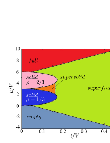
Figure 1: Phase diagram in the grand-canonical ensemble for $c_{2}=V/k_{\rm B}T=50.0$, which corresponds to the low-temperature phase.

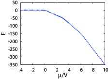
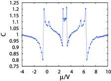
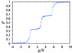
Figure 2: Internal energy, specific heat and particle density as a function of $\mu/V$ for $c_{1}=5$ and $c_{2}=50$ $(t/V=0.1)$ in the grand-canonical ensemble. System size $L=24$.

We first show the phase structure of the system in the grand-canonical ensemble. To investigate the phase structure, we measured the internal energy $E$, the specific heat $C$, the particle density $\rho$, etc, which are defined as $E=\langle H\rangle/L^{3}$, $C=\langle(H-E)^{2}\rangle/L^{3}$ and $\rho=\langle n_{i}\rangle$, where $L$ is the linear system size. We numerically studied the system at various $T$’s and found that the phase diagram changes continuously. For the low-$T$ phase, we set $c_{2}=50$ and obtain the phase diagram in the $t/V-\mu/V$ plane. See Fig.1. There are full and empty states in the phase diagram, in which all sites of the system are occupied or empty, respectively. For $t/V\ll 1$, there appear “solid” states with the density $\rho={1\over 3}$ and $\rho={2\over 3}$. It is easily seen that these states in which one of three sites is filled (empty) in a $\sqrt{3}\times\sqrt{3}$ ordering have minimum energy for $t/V\ll 1$Met . As $t/V$ is increased, there appear the SS and superfluid (SF) states. The obtained phase diagram in Fig.1 is essentially the same with that of the system in the 2D triangular lattice at $T=0$triangle . The three dimensionality of the present system preserves the ordered states at $T=0$ in 2D up to the low but finite $T$.

In the following, we shall exhibit the MC calculations that derived the above phase diagram in Fig.1. First in Fig.2, we show $E$, $C$ and $\rho$ as a function of $\mu$ for $c_{1}=5$ and $c_{2}=50$, i.e., $t/V=0.1$. It is obvious that there is a particle-hole symmetry. Singular behavior of $C$ indicates that there are totally six phase transitions and the step-function like behavior of $\rho$ indicate that phase transitions at $\mu/V\simeq 0,3$ and $6$ are of first order.

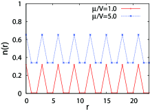
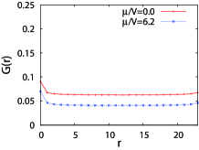
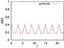
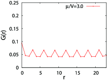
Figure 3: Correlation functions $n(r)$ and $G(r)$ in various phases for $c_{1}=5$ and $c_{2}=50$ $(t/V=0.1)$ in the grand-canonical ensemble. $L=24$.

In order to verify the physical meaning of each phase, we measured the particle-density correlation function $n(r)$ and the HC boson correlation function $G(r)$, which are defined as follows,

$$n(r)=\langle\phi^{\dagger}_{i}\phi_{i}\phi^{\dagger}_{i+r}\phi_{i+r}\rangle,\;\;G(r)=\langle\phi^{\dagger}_{i}\phi_{i+r}\rangle.$$ (7)

It is expected that in the solid states with $\rho={1\over 3}$ and ${2\over 3}$, $n(r)$ exhibits a specific correlation with $3a$ periodicity ($a=$ lattice spacing), whereas vanishing superfluid correlation, i.e., $G(r)\rightarrow 0$ for $r\rightarrow$ large. On the other hand in the superfluid state, $n(r)$ exhibits a homogeneous distribution of bosons and there exists a finite superfluid correlation. Supersolid has finite correlation of the both $n(r)$ and $G(r)$. We have verified all of the above expectations by the MC simulations, and here we show some of the results in Fig.3. In the solid states, the HC bosons are localized in a specific pattern to avoid repulsions and as a result a density wave appears. Then, the superfluid correlation decays very rapidly there. The superfluid is a homogeneous state with nonvanishing HC boson LRO. On the other hand in the SS, both the density wave and HC boson LRO appear.

Snapshots are useful to get an intuitive physical picture of each phase. In Fig.4, we show snapshots of particle density of each phase. In the solid states, particles are localized, whereas in the superfluid a homogeneous state is realized. In the SS, the high-density region fluctuates and localized domains come to overlap with each other.

Figure 4: Snapshot of density $n(r)$ in various phases for $c_{1}=5$ and $c_{2}=50$ $(t/V=0.1)$ in the grand-canonical ensemble. Upper left: $\rho={1\over 3}$ solid, Upper right: $\rho={1\over 3}$ solid, Lower left: SF, and Lower right: SS.

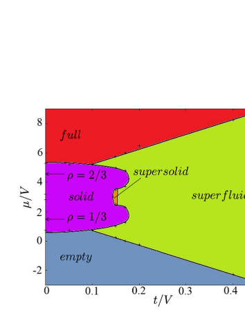
Figure 5: Phase diagram in the grand-canonical ensemble for $c_{2}=V/k_{\rm B}T=10.0$

It is interesting to see how the phase diagram changes as $T$ is raised. As we are studying the 3D system, we can address this interesting problem. We show the phase diagram of the system with $c_{2}=\beta V=10.0$ in Fig.5. It is obvious that the parameter regions of the SS and also SF are getting small compared to those at low $T$. Phase boundary of the two solids with $\rho={1\over 3}$ and ${2\over 3}$ becomes obscure. The calculated specific heat $C$ and the particle density $\rho$ are show in Fig.6 as a function of the chemical potential. For $c_{1}=1.0$ and $c_{2}=10.0$, there are two sharp peaks in $C$ at $\mu/V\simeq 1.0$ and $5.5$, which are related with each other by the particle-hole symmetry, and correspond to the empty-solid/solid-full phase transitions. There also exists a small V-shape hollow at $\mu/V\simeq 3.0$, i.e., $\rho\simeq 0.5$. Calculation of $\rho$ exhibits rather smooth behavior without the sharp step-function like discontinuities that exist at low $T$. The obtained correlation functions in Fig.7 indicate that a mixed state of the two solids with $\rho={1\over 3}$ and $\rho={2\over 3}$ appears for $1.0<\mu/V<5.5$ and the density of each solid depends on value of $\mu/V$.

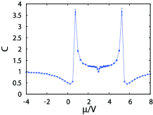
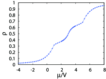
Figure 6: Specific heat and density as a function of $\mu/V$ for $c_{1}=1.0$ and $c_{2}=10$ (i.e., $t/V=0.1$).

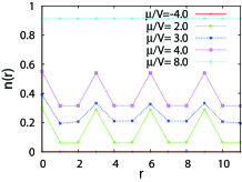
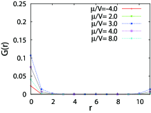
Figure 7: Correlations of density and particle for $c_{1}=1.0$ and $c_{2}=10$.

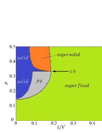
Figure 8: Phase diagram in the canonical ensemble for $c_{2}=50.0$.

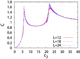
Figure 9: Specific heat $C$ for $t/V=0.1$ and $\rho=0.5$ as a function of $c_{2}$. There exist two peaks indicating two second-order phase transitions.

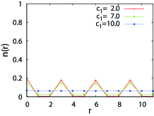
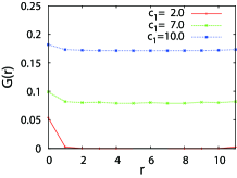
Figure 10: Number and HCB correlation functions in the canonical ensemble for $c_{2}=50.0$ and $\rho=0.25$.

Let us turn to the phase diagram of the system in the canonical ensemble. We use the MC simulations with local updates that conserve the total boson number. We consider the low-$T$ case with $c_{2}=50$ and show the phase diagram in the $t/V-\rho$ plane in Fig.8. We show only the region $0<\rho<0.5$ because the particle-hole symmetry gives the other half of the parameter region. For small $t/V$ and $0.15<\rho<0.85$, the system exists in the solid state. From the above study on the system in the grand-canonical ensemble, this state can be regarded as a mixture of the solids with $\rho={1\over 3}$ and ${2\over 3}$. From $\rho=0.33$ to 0.67 and $0.1<t/V<0.2$, the SS appears as in the grand-canonical ensemble. This result seems to be in sharp contrast with the phase diagram in the 2D triangular lattice at $T=0$, in which the SS appear even for very small $t/V$triangle . This apparent discrepancy is closely related with how the SS evolves as $T$ is raised. To see this, we study the system with $t/V=c_{1}/c_{2}=0.1$ and $\rho=0.5$ by varying the value of $\beta$. See Fig.9, in which the specific heat $C$ is shown as a function of $c_{2}$. The result shows that there exist two phase transitions at $c_{2}\simeq 8.0$ and $22$ both of which are of second order. By studying the correlation functions, we found that as $T$ is raised, the phase transition from the SS to the solid state takes place first at $c_{2}\simeq 22$ and then at $c_{2}\simeq 8.0$ to the state without any long-range orders. See also Figs.1 and 5. Therefore the obtained finite-$T$ phase diagram is consistent with that at $T=0$ in 2D. It should be remarked that in the 2D system at finite-$T$ with $\rho=0.5$, corresponding phase transitions take place almost simultaneously2DT . In Fig.10, we show the correlation functions $n(r)$ and $G(r)$ for $c_{2}=50.0$ and $\rho=0.25$ in the canonical ensemble.

In the phase diagram in the canonical ensemble shown in Fig.8, the phase-separated (PS) state also exists, which does not appear in the grand-canonical ensemble. Similar result was obtained for the system of the 2D triangular lattice at $T=0$triangle . In the grand-canonical ensemble, the most stable state appears for each value of the chemical potential, and an inhomogeneous state is sometimes difficult to be observed.

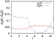
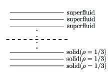
Figure 11: (Left)Number and HC boson correlation functions in the layered direction in the canonical ensemble for $c_{2}=50.0$ and $\rho=0.25$. (Right)Sketch of a PS state in 3D.

It is interesting how the PS state is realized in the present stacked triangular latticePSsquare . In the 2D triangular lattice, the PS state is composed of domains of the solid and those of the SF. As shown in Fig.10, the density and HC boson correlations for $c_{1}=7.0$ seem to imply that the SS is realized there, i.e., the solid-like behavior of $n(r)$ and the SF-like behavior of $G(r)$. Then we studied the correlations in the layered direction, and show the results in Fig.11. The results indicate that SF layers and solid layers appear separately as depicted in Fig.11 in contrast to the 2D case.

In conclusion, we have studied finite-$T$ phase diagram of the HC boson system in the stacked triangular lattice. There exist various phases in the phase diagram and the obtained results are consistent with the phase structure of the HC boson system in the triangular lattice at $T=0$. We also found that the SS first loses the superfluidity and then the density-wave order as $T$ is raised.