Chiral Symmetry Breaking in Planar QED in External Magnetic Fields

Abstract

We investigate planar quantum electrodynamics (QED) with two degenerate staggered fermions in an external magnetic field on the lattice. We argue that in external magnetic fields there is dynamical generation of mass for two-dimensional massless Dirac fermions in the weak-coupling region. We extrapolate our lattice results to the quantum Hall effect in graphene.

I Introduction

Quantum electrodynamics (QED) in 2+1 dimensions is interesting as a model for several condensed matter systems. In fact, quantum electrodynamics with two massless Dirac fermions could be relevant to describe the low-energy excitations of a single sheet of carbon atoms arranged in a honeycomb structure called “graphene” Novoselov et al. (2004, 2005). When graphene is immersed in a transverse magnetic field, the presence of Landau levels at zero energy leads to half-integer quantum Hall effect. Moreover, for very strong magnetic fields there is experimental evidence for the dynamical generation of a gap, which signals the spontaneous breaking of the chiral symmetry. In fact, it has been suggested that a magnetic field is a strong catalyst of chiral symmetry breaking in spinorial QED Gusynin et al. (1994, 1995) even at the weakest attractive interaction between fermions.
The aim of the present paper is to investigate, by means of non-perturbative Monte Carlo simulations, planar quantum electrodynamics (QED) with two degenerate staggered fermions in an external magnetic field. To make contact with the physical planar systems, we choose to work in the weak-coupling region. A preliminary account of the results discussed in the present paper has been published in Ref. Cea et al. (2011).
The plan of the paper is as follows. In Sect. II, for completeness, we briefly discuss our method to introduce background fields on the lattice and compare with different approaches in the literature. Section III is devoted to the discussion of our lattice Euclidean action. In Sect. IV we present the results of our numerical simulations for two different values of the gauge coupling in the weak-coupling region. In Sect. V we extrapolate our results to the physical relevant case of the quantum Hall effect in graphene. Finally, our conclusions are relegated in Sect. VI.

II Background fields on the lattice

The study of lattice gauge theories with an external background field has been pioneered in Ref. Damgaard and Heller (1988a, b) for the U(1) Higgs model in an external electromagnetic field. In the continuum a background field can be introduced by writing:

$$A_{\mu}(x)\;\rightarrow\;A_{\mu}(x)\;+\;A^{\text{ext}}_{\mu}(x)\;.$$ (1)

In the lattice approach one deals with link variables $U_{\mu}(x)$. Accordingly, on the lattice Eq. (1) becomes:

$$U_{\mu}(x)\;\rightarrow\;U_{\mu}(x)\,U^{\text{ext}}_{\mu}(x)\;,$$ (2)

where $U^{\text{ext}}_{\mu}(x)$ is the lattice version of the background field $A^{\text{ext}}_{\mu}(x)$. As a consequence the gauge action gets modified as:

$$S_{G}[U]\;\rightarrow\;S_{G}[U]\;+\delta\,S[U,U^{\text{ext}}]\;,$$ (3)

where $\delta\,S[U,U^{\text{ext}}]$ takes into account the influence of the external field Smit and Vink (1987); Ambjorn et al. (1989, 1990); Kajantie et al. (1999); Buividovich et al. (2009); D’Elia et al. (2010); Bali et al. (2012); Ilgenfritz et al. (2012). An alternative method, which is equivalent in the continuum limit, is based on the observation that an external background field can be introduced via an external current Cea and Cosmai (1991a, b); Levi and Polonyi (1995); Ogilvie (1998); Chernodub et al. (2001):

$$J^{\text{ext}}_{\mu}\;=\;\partial_{\nu}\;F^{\text{ext}}_{\nu\mu}\;.$$ (4)

The gauge action gets modified in an obvious manner:

$$S_{G}\;\rightarrow\;S_{G}\;+\;S_{B}\;,$$ (5)

where:

$$S_{B}\; =\;\int dx\;J^{\text{ext}}_{\mu}(x)\;A_{\mu}(x)$$

$$=\;-\;\frac{1}{2}\;\int dx\;F^{\text{ext}}_{\nu\mu}(x)\,F_{\nu\mu}(x)\;.$$ (6)

The background action $S_{B}$ can be now easily discretized on the lattice.
The main disadvantage of this approach resides on the fact that it cannot be extended to the case of non-Abelian gauge group in a gauge-invariant way. To overcome this problem, the background field on the lattice can be implemented by means of the gauge invariant lattice Schrödinger functional Cea et al. (1997); Cea and Cosmai (1999):

$${\mathcal{Z}}[U^{\mathrm{ext}}_{k}]=\int{\mathcal{D}}U\;e^{-S_{G}}\;,$$ (7)

where the functional integration is extended over links on a lattice with the hypertorus geometry and satisfying the constraints ($x_{t}$ is the temporal coordinate)

$$U_{k}(x)|_{x_{t}=0}=U^{\mathrm{ext}}_{k}(\vec{x})\;.$$ (8)

We also impose that links at the spatial boundaries are fixed according to Eq. (8). In the continuum this last condition amounts to the requirement that fluctuations over the background field vanish at infinity.
The effects of dynamical fermions can be accounted for quite easily. In fact, when including dynamical fermions, the lattice Schrödinger functional in presence of a static external background gauge field becomes Cea et al. (2004)

$$\mathcal{Z}[U^{\mathrm{ext}}_{k}] = \int_{U_{k}(L_{t},\vec{x})=U_{k}(0,\vec{x})=U^{\text{ext}}_{k}(\vec{x})}\mathcal{D}U\,{\mathcal{D}}\psi\,{\mathcal{D}}\bar{\psi}e^{-(S_{G}+S_{F})}$$ (9)

$$= \int_{U_{k}(L_{t},\vec{x})=U_{k}(0,\vec{x})=U^{\text{ext}}_{k}(\vec{x})}\mathcal{D}Ue^{-S_{G}}\,\det M\,,$$

where $S_{F}$ is the fermionic action and $M$ is the fermionic matrix. Notice that the fermionic fields are not constrained and the integration constraint is only relative to the gauge fields. This leads to the appearance of the gauge invariant fermionic determinant after integration on the fermionic fields. As usual we impose on fermionic fields periodic boundary conditions in the spatial directions and antiperiodic boundary conditions in the temporal direction.

III Lattice planar QED in external magnetic field

We are interested in planar quantum electrodynamics with $N_{f}=2$ degenerate Dirac fields in an external constant magnetic field. As it is well known, Dirac fields are described non-perturbatively by the lattice Euclidean action using $N$ flavours of staggered fermion fields $\overline{\chi},\chi$ Hands et al. (2002):

$$S=S_{G}+\sum_{i=1}^{N}\sum_{n,m}\overline{\chi}_{i}(n)M_{n,m}\chi_{i}(m)\;,$$ (10)

where $S_{G}$ is the gauge field action and the fermion matrix is given by:

$$M_{n,m}[U]=$$

$$\sum_{\nu=1,2,3}\frac{\eta_{\nu}(n)}{2}\left\{U_{\nu}(n)\delta_{m,n+\hat{\nu}}-U_{\nu}^{\dagger}(m)\delta_{m,n-\hat{\nu}}\right\}+m_{0}\delta_{m,n}\;,$$

$$\;\;\;\;\eta_{\nu}(n)=(-1)^{n_{1}+\ldots+n_{\nu-1}}\;,$$ (11)

where $m_{0}$ is the bare fermion mass. Here we adopt the compact formulation for the electromagnetic field (for a detailed account see Ref. Fiore et al. (2005)). The gauge action is:

$$S_{G}[U]=\beta\sum_{n,\mu<\nu}{\left[1-\frac{1}{2}\left(U_{\mu\nu}(n)+U_{\mu\nu}^{\dagger}(n)\right)\right]}\;,$$ (12)

where $U_{\mu\nu}(n)$ is the plaquette and $\beta=\frac{1}{e^{2}}$. The action Eq. (10) with $N=1$ flavours of staggered fermions corresponds to $N_{f}=2$ flavours of 4-component Dirac fermions $\Psi$ Burden and Burkitt (1987).
To introduce an external magnetic field, we shall follow the lattice Schrödinger functional described in Sect. III (for a different approach see Ref. Alexandre et al. (2001)). Accordingly, in the functional integration over the lattice links we constrain the spatial links belonging to the time slice $x_{t}=0$ to

$$U_{k}(\vec{x},x_{t}=0)=U^{\text{ext}}_{k}(\vec{x})\,,\,\,\,\,\,k=1,2\,\,,$$ (13)

$U^{\text{ext}}_{k}(\vec{x})$ being the lattice version of the external continuum gauge potential. Since our background field does not vanish at infinity, we must also impose that, for each time slice $x_{t}\neq 0$, spatial links exiting from sites belonging to the spatial boundaries are fixed according to Eq. (13).
The continuum gauge potential giving rise to a constant magnetic field is given by:

$$A^{\text{ext}}_{k}(\vec{x})=\delta_{k,2}\ x_{1}H\;,$$ (14)

so that:

$$U^{\text{ext}}_{1}(\vec{x})=1\,,\,U^{\text{ext}}_{2}(\vec{x})=\cos(eHx_{1})+i\sin(eHx_{1})\,.$$ (15)

Since our lattice has the topology of a torus, the magnetic field turns out to be quantized:

$$eH=\frac{2\pi}{L}n_{\text{ext}}\;,\;\;\;n_{\text{ext}}\,\,\,{\text{integer}}\;,$$ (16)

where $L$ is the lattice size. We recall once more that the fermion fields are unconstrained and satisfy antiperiodic boundary conditions in the timelike direction and periodic boundary conditions in the spatial directions.
Our numerical results were obtained by simulating the action Eq. (10) on $L^{3}$ lattice using standard hybrid Monte Carlo algorithm.

IV Chiral symmetry breaking

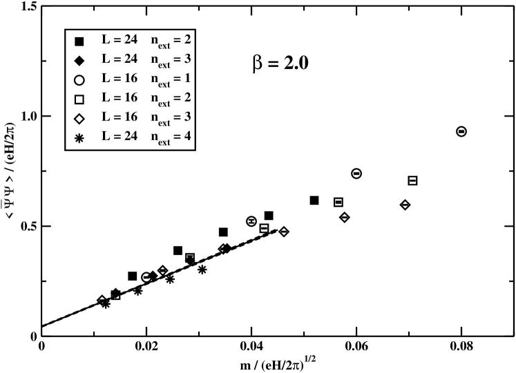
Figure 1: Scaled chiral condensate versus the scaling variable $x=\frac{m_{0}}{\sqrt{eH/2\pi}}$ for $\beta=2.0$. The continuum line is the linear fit of the data Eqs. (18) and (19) in the scaling region $0<x\lesssim 0.045$.

We are looking for the dynamical generation of a gap for massless fermions. This corresponds to a non-zero chiral condensate $\langle\overline{\Psi}\Psi\rangle$ in the chiral limit. Our strategy is to measure the fermion condensate with a small bare fermion mass $m_{0}$ and then perform the massless limit $m_{0}\rightarrow 0$ in presence of a constant external magnetic field. Our simulations have been performed in the weak-coupling region with two different values of the gauge coupling $\beta=2.0$ and $\beta=2.5$. In fact, in the weak-coupling region we expect that the effects of the Coulomb interactions could be neglected allowing to extrapolate our numerical results to physical planar systems.
We have performed simulations on lattices with $L=16,$ 24 and $0.005\leqslant m_{0}\leqslant 0.03$ with different strengths of the external magnetic field labelled by the integer $n_{\text{ext}}$ according to Eq. (16). For each parameter set, to allow thermalization we discard $10000$ sweeps for $L=16$ and $7000$ sweeps for $L=24$. We collect about $50000$ hybrid Monte Carlo trajectories. To optimize the performance of the hybrid Monte Carlo algorithm, we tuned the simulation parameters to give an acceptance of about $80\%$. The chiral condensate $\langle\overline{\Psi}\Psi\rangle$ was estimated by the stochastic source method. In order to reduce autocorrelation effects, measurements were taken every 10 steps for $L=16$ and every 5 steps for $L=24$ . Data were analyzed by the jackknife method combined with binning.
In Fig. 1 we display the chiral condensate for different values of the lattice size, bare fermion mass, and magnetic field strength for $\beta=2.0$ . Note that, according to Eq. (16), the strength of the external magnetic field depends on $n_{\text{ext}}$ as well on the lattice size $L$. To avoid lattice discretization and finite volume effects, we have fixed the magnetic field strength such that the magnetic length satisfies the bounds:

$$1\ll\sqrt{{\frac{2\pi}{eH}}}\;\ll\;L\;.$$ (17)

We expect that in the continuum limit the relevant scale is set by the magnetic length. This means that the rescaled chiral condensate $\frac{\langle\overline{\Psi}\Psi\rangle}{\frac{eH}{2\pi}}$ would depend only on the scaling variable $x\equiv\frac{m_{0}}{\sqrt{\frac{eH}{2\pi}}}$. Actually, from Fig. 1, where we display the rescaled chiral condensate versus the dimensionless scaling variable $x$, we see that in the region $x\gtrsim 0.05$ data are rather scattered. However, in the region $x\lesssim 0.05$ our data seem to collapse to an universal curve. This means that in this region, that we shall call the scaling region, the rescaled chiral condensate depends only on the scaling variable $x$. This allows us to extract the chiral condensate in the chiral limit $m_{0}\rightarrow 0$, which corresponds to $x\rightarrow 0$, for a fixed strength on the external magnetic field. In fact, we try to fit the data in the scaling region $0<x\lesssim 0.045$ according to:

$$\frac{\langle\overline{\Psi}\Psi\rangle}{\frac{eH}{2\pi}}\;=\;a_{0}\,+\,a_{1}\,x\;\;,\;\;\;\;\;x=\frac{m_{0}}{\sqrt{\frac{eH}{2\pi}}}\,.$$ (18)

The best fit of the data to Eq. (18) in the scaling region gives:

$$a_{0}\,=\,0.04399\,\pm\,0.00131\;\;,\;\;\;\;\;a_{1}\,=\,9.759\,\pm\,0.055\;\;,\;\;\;\;\;$$ (19)

$$\chi^{2}_{\rm d.o.f.}\;\simeq 747\;.$$

We note, however, that there are sizable violations of our scaling law as implied by the huge reduced chi-square. We believe that these scaling violations are mainly due to the fermion interactions with the electromagnetic field, which could introduce a spurious dependence of the scaled chiral condensate on the dimensionless ratio $\frac{e^{2}}{\sqrt{\frac{eH}{2\pi}}}$. To check this point, we have performed numerical simulations by increasing the gauge coupling $\beta$ (which corresponds to a smaller $e^{2}$). In fact, in Fig. 2 we display the results of our simulations for $\beta=2.5$. Again we see that the data for the rescaled chiral condensate seem to collapse to to an universal curve in the scaling region $x\lesssim 0.05$. Moreover, comparing Fig. 2 with Fig. 1 it is evident that the scaling violation are greatly reduced allowing a better extrapolation to the chiral limit. Fitting the data to Eq. (18) we find:

$$a_{0}\,=\,0.03544\,\pm\,0.00084\;\;,\;\;\;\;\;a_{1}\,=\,8.382\,\pm\,0.032\;\;,\;\;\;\;\;$$

$$\chi^{2}_{\rm d.o.f.}\;\simeq 466\;.$$ (20)

Even though the reduced chi-square is quite large, we believe that our results are robust enough to allow the extrapolation of the chiral condensate to the chiral limit. As a consequence, we conclude that in the chiral limit the external magnetic field does induce a non-zero chiral condensate. From Eqs. (18) and (IV) we find for the chiral condensate in the massless limit:

$$\langle\overline{\Psi}\Psi\rangle\;=\;\frac{eH}{2\pi}\left(0.03544\,\pm\,0.00084\right)\,.$$ (21)

The non-zero value of the chiral condensate can be interpreted as the generation of a dynamical fermion mass which, in principle, can be extracted from the non-zero chiral condensate in the chiral limit.

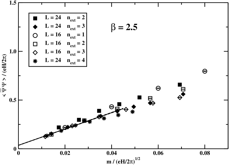
Figure 2: Scaled chiral condensate versus the scaling variable $x=\frac{m_{0}}{\sqrt{eH/2\pi}}$ for $\beta=2.5$. The continuum line is the linear fit of the data Eqs. (18) and (19) in the scaling region $0<x\lesssim 0.045$.

In the determination of the value of the chiral condensate, as given in Eq. (21), we neglected a possible contribution present even in absence of the magnetic field. Indeed, in Ref. Armour et al. (2011) it was shown that the chiral condensate is non-zero in the weak-coupling regime of compact planar QED even at zero external magnetic field. In order to check the possible impact of this zero-field contribution on our determination of the chiral condensate, we observe that in Ref. Fiore et al. (2005) two of us found $\beta^{2}\langle\overline{\Psi}\Psi\rangle\;\approx\;1.5\times 10^{-3}$ for $H=0$ on a lattice with $L=12$. This result implies, for $\beta=2.5$, that $\langle\overline{\Psi}\Psi\rangle\;=\;0.00024$, in lattice units. In this work the smallest value of the chiral condensate induced by an external magnetic field is obtained for $n_{\text{ext}}=1$ and $L=16$, which implies $eH/(2\pi)=0.0625$ and therefore, through Eq. (21), $\langle\overline{\Psi}\Psi\rangle\;=\;0.002215$. The latter value is one order of magnitude bigger than the former and cannot be attributed to finite size effects, in consideration of the similar lattice sizes adopted in the two determinations. This allows us to safely neglect the zero-field contribution to the chiral condensate.

V Extrapolation to Graphene

In this Section we attempt to apply our numerical determination of the chiral condensate in the chiral limit to graphene immersed in a transverse magnetic field. For the reader’s convenience, we briefly discuss the remarkable quantum Hall effect in graphene.
As is well known, graphene is a flat monolayer of carbon atoms tightly packed in a two dimensional honeycomb lattice consisting of two interpenetrating triangular sublattices (for a review, see Ref. Castro Neto et al. (2009)). Indeed, the structure of graphene has attracted considerable attention since the low-energy excitations are given by two Pauli spinors $\Psi_{\pm}$ which satisfy the massless two-dimensional Dirac equation with the speed of light replaced by the Fermi velocity $v_{F}\simeq 1.0\,10^{8}\,$ cm/s. The Pauli spinors can be combined into a single Dirac spinor $\Psi=\left(\begin{array}[]{c}\Psi_{+}\\ \Psi_{-}\end{array}\right)$. Taking into account the real spin degeneracy, we see that the low-energy dynamics of graphene can be accounted for by $N_{f}=2$ massless Dirac fields Drut and Lähde (2009a, b).

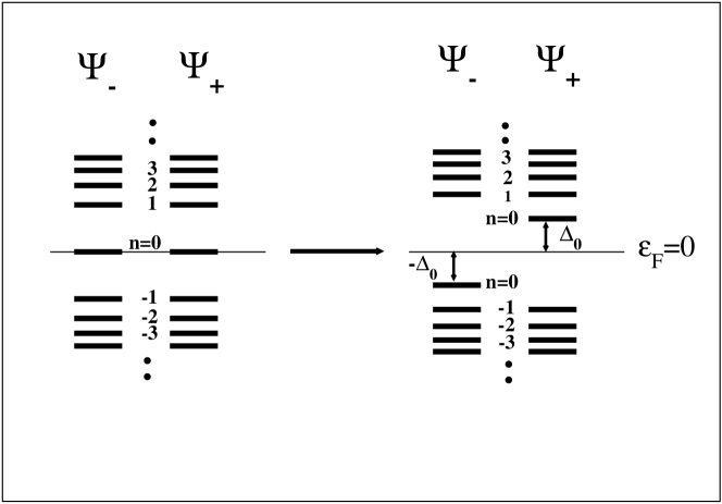
Figure 3: Schematic spectrum of Landau levels of graphene in applied magnetic field (left). Landau levels with dynamical generation of a gap $\Delta_{0}$ (right). The Fermi level is at $\varepsilon_{F}=0$.

When graphene is immersed in a transverse magnetic field, the relativistic massless dispersion of the electronic wave functions results in non-equidistant Landau levels :

$$\varepsilon_{n}={\rm sign}(n)\sqrt{2|n|\hslash\frac{v_{F}^{2}}{c}eH}\,,\,\;\;\;n\,=\,0\,,\,\pm\,1\,,\,\pm\,2\;...$$ (22)

where $eH>0$, $e$ being the elementary charge (see Fig. 3, left). The presence of anomalous Landau levels at zero energy, $\varepsilon_{0}=0$, leads to half-integer quantum Hall effect corresponding to quantized filling factor $\nu=\pm 2\,,\,\pm 6\,,\,\pm 10\,\,...$.
Recent studies of quantum Hall effect in graphene in very strong magnetic field $H\gtrsim 20\,T$ (1 T = $10^{4}\,$ gauss) have revealed new quantum Hall states corresponding to filling factor $\nu=0\,,\,\pm 1\,,\,\pm 4$ Zhang et al. (2006); Jiang et al. (2007). The new plateaus at $\nu=0\,\,,\,\pm 4$ can be explained by Zeeman spin splitting. On the other hand the $\nu=\pm 1$ plateaus are associated with the spontaneous breaking of the symmetry in the $n=0$ Landau levels (the so-called valley symmetry). Indeed, these states are naturally explained if there is dynamical generation of a gap $\Delta_{0}$ (see Fig. 3, right).
The gap $\Delta_{0}$ can be extracted from the measured activation energy. In fact, in Fig. 4 we display the measured activation energy gap $\Delta E(\nu=1)$ as a function of the magnetic field for the $\nu=1$ quantum Hall states Jiang et al. (2007). To extract $\Delta_{0}$ from the activation energy data, we need to take care of the Zeeman energy which for strong magnetic fields is no more negligible. To this end, we may fit the data to:

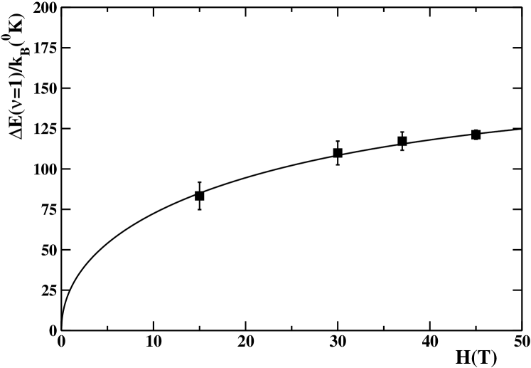
Figure 4: The measured activation energy gap $\Delta E(\nu=1)$ as a function of magnetic field for the quantum Hall states at filling factor $\nu=1$. The data have been extracted from Fig. 2 of Ref. Jiang et al. (2007). The continuum line is the best fit of the experimental data to Eq. (23).

$$\Delta E(\nu=1)=2\,\left(\Delta_{0}(H)\,+\,\frac{g}{2}\mu_{B}\,H\right)\;,$$ (23)

where $\mu_{B}$ is the Bohr magneton, $g=2$ and $\Delta_{0}(H)\sim\sqrt{H}$ Jiang et al. (2007). Figure 4 shows that, indeed, our Eq. (23) gives an excellent fit to the data. We find:

$$\Delta_{0}(H)\,=\,(13.57\,\pm 0.28)\;{\rm K}\,k_{B}\;\sqrt{H(T)}\;,$$ (24)

where $H(T)$ means that the magnetic field is measured in Tesla.
Our strategy is, now, to relate the gap $\Delta_{0}$ to the chiral condensate. After that, using our determination of the chiral condensate on the lattice, we will estimate the gap and compare with the experimental determination Eq. (24).
To this purpose we follow Ref. Cea (2012), where the hypothesis of rearrangement of the Dirac sea of graphene in an external magnetic field was used and the electron-electron Coulomb interactions were neglected. Note that in graphene the electron-electron Coulomb interaction, $e^{2}/r$, in general is not small, so that this approximation could be questionable. A direct calculation gives Cea (2012):

$$\langle\overline{\Psi}\Psi\rangle\;=\;-\,2\,\Delta_{0}\,\frac{\hslash ceH}{2\pi}\frac{1}{\sqrt{2\hslash\frac{v_{F}^{2}}{c}eH}}\frac{\Gamma(\frac{1}{2})}{\sqrt{\pi}}\;\zeta(\frac{1}{2},1+\alpha^{2})\;,$$

$$\;\;\;\;\;\;\;\alpha\;=\;\frac{\Delta_{0}}{\sqrt{2\hslash\frac{v_{F}^{2}}{c}eH}}\;\;,$$ (25)

where $\Gamma(x)$ is the Euler gamma function and $\zeta(x,y)$ is the generalized Riemann Zeta function. For small gap, we may expand to the first order in $\Delta_{0}$. Using $\Gamma(\frac{1}{2})=\sqrt{\pi}$ and $\zeta(x,1)=\zeta(x)$, we get:

$$\frac{\langle\overline{\Psi}\Psi\rangle}{\frac{\hslash ceH}{2\pi}}\;\simeq\;-\,2\,\Delta_{0}\;\frac{1}{\sqrt{2\hslash\frac{v_{F}^{2}}{c}eH}}\;\zeta(\frac{1}{2})\;.$$ (26)

This last equation relates the gap $\Delta_{0}$ to the rescaled dimensionless chiral condensate. Using our determination on the lattice for the rescaled chiral condensate, we obtain:

$$\Delta_{0}\;\simeq\;\,-\,\frac{\sqrt{\pi}}{\zeta(\frac{1}{2})}\;\;\sqrt{\frac{\hslash\frac{v_{F}^{2}}{c}eH}{2\pi}}\;\;a_{0}\;,$$ (27)

where $a_{0}$ is given in Eq. (IV). Finally, with the experimental value for the Fermi velocity we get:

$$\Delta_{0}(H)\,\simeq\,2.6\;\;{\rm K}\,k_{B}\;\sqrt{H(T)}.$$ (28)

Comparing Eq. (28) with Eq. (24), we see that our estimate of the gap is about a factor five smaller than the experimental data. However, it is remarkable that we are able to reproduce the dependence on the external magnetic field $\Delta_{0}\sim\sqrt{H}$.

VI Conclusions

We investigated planar quantum electrodynamics with two degenerate staggered fermions in an external magnetic field on the lattice. Our numerical results seem to indicate that in an external magnetic field there is a non-zero chiral condensate in the chiral limit pointing to a dynamical generation of mass for two-dimensional massless Dirac fermions.

We performed our simulations in the weak-coupling regime of the compact formulation of the lattice gauge action. As discussed in Ref. Armour et al. (2011), the non-compact formulation of the theory could have a different continuum limit than the compact one, the signature of this being the different magnetic monopole dynamics, which in compact QED leads to an enhanced chiral condensate. As a matter of fact, in the compact theory the chiral condensate is non-zero in the strong-coupling regime and undergoes a crossover to a non-zero value in the weak-coupling regime, while in the weak-coupling regime of the non-compact theory it is compatible with zero. Although we believe that the numerical impact of this possible different behaviour in the continuum should be negligible to our purposes, we plan to explicitly check this point by performing numerical simulations with the non-compact lattice gauge action. This will also permit us to make a comparison with the results of Ref. Alexandre et al. (2001), where a different approach was adopted to introduce the background magnetic field on the lattice.

We also tried to extrapolate our lattice results to the quantum Hall effect in graphene, since the low energy dynamics of graphene is described by $N_{f}=2$ massless Dirac fermions. Our non-perturbative Monte Carlo simulations allowed to confirm the dynamical breaking of the valley symmetry in the lowest Landau levels. Moreover, even though we greatly underestimate the dynamical gap, we were able to reproduce the dependence of the dynamical gap on the strength of the external magnetic field.

References

- Novoselov et al. (2004) K. S. Novoselov, A. K. Geim, S. V. Morozov, D. Jiang, Y. Zhang, S. V. Dubonos, I. V. Grigorieva, and A. Firsov, Science 306, 666 (2004).
- Novoselov et al. (2005) K. Novoselov, D. Jiang, F. Schedin, T. J. Booth, V. V. Khotkevich, S. V. Morozov, and A. K. Geim, PNAS 102, 10451 (2005).
- Gusynin et al. (1994) V. Gusynin, V. Miransky, and I. Shovkovy, Phys. Rev. Lett. 73, 3499 (1994), arXiv:hep-ph/9405262 [hep-ph] .
- Gusynin et al. (1995) V. Gusynin, V. Miransky, and I. Shovkovy, Phys. Rev. D52, 4718 (1995), arXiv:hep-th/9407168 [hep-th] .
- Cea et al. (2011) P. Cea, L. Cosmai, P. Giudice, and A. Papa, PoS LATTICE2011, 307 (2011), arXiv:1109.6549 [hep-lat] .
- Damgaard and Heller (1988a) P. H. Damgaard and U. M. Heller, Phys. Rev. Lett. 60, 1246 (1988a).
- Damgaard and Heller (1988b) P. H. Damgaard and U. M. Heller, Nucl. Phys. B 309, 625 (1988b).
- Smit and Vink (1987) J. Smit and J. C. Vink, Nucl. Phys. B286, 485 (1987).
- Ambjorn et al. (1989) J. Ambjorn, V. Mitrjushkin, V. Bornyakov, and A. Zadorozhnyi, Phys. Lett. B225, 153 (1989).
- Ambjorn et al. (1990) J. Ambjorn, V. Mitrjushkin, and A. Zadorozhnyi, Phys. Lett. B245, 575 (1990).
- Kajantie et al. (1999) K. Kajantie, M. Laine, J. Peisa, K. Rummukainen, and M. E. Shaposhnikov, Nucl. Phys. B544, 357 (1999), arXiv:hep-lat/9809004 [hep-lat] .
- Buividovich et al. (2009) P. Buividovich, M. Chernodub, E. Luschevskaya, and M. Polikarpov, Phys. Rev. D80, 054503 (2009), arXiv:0907.0494 [hep-lat] .
- D’Elia et al. (2010) M. D’Elia, S. Mukherjee, and F. Sanfilippo, Phys. Rev. D82, 051501 (2010), arXiv:1005.5365 [hep-lat] .
- Bali et al. (2012) G. Bali, F. Bruckmann, G. Endrodi, Z. Fodor, S. Katz, et al., JHEP 1202, 044 (2012), arXiv:1111.4956 [hep-lat] .
- Ilgenfritz et al. (2012) E.-M. Ilgenfritz, M. Kalinowski, M. Muller-Preussker, B. Petersson, and A. Schreiber, (2012), arXiv:1203.3360 [hep-lat] .
- Cea and Cosmai (1991a) P. Cea and L. Cosmai, Phys. Rev. D 43, 620 (1991a).
- Cea and Cosmai (1991b) P. Cea and L. Cosmai, Phys. Lett. B264, 415 (1991b).
- Levi and Polonyi (1995) A. Levi and J. Polonyi, Phys. Lett. B357, 186 (1995), arXiv:hep-lat/9505007 [hep-lat] .
- Ogilvie (1998) M. Ogilvie, Nucl. Phys. Proc. Suppl. 63, 430 (1998), arXiv:hep-lat/9709127 [hep-lat] .
- Chernodub et al. (2001) M. Chernodub, E.-M. Ilgenfritz, and A. Schiller, Phys. Rev. D64, 114502 (2001), arXiv:hep-lat/0106021 [hep-lat] .
- Cea et al. (1997) P. Cea, L. Cosmai, and A. Polosa, Phys. Lett. B392, 177 (1997), arXiv:hep-lat/9601010 [hep-lat] .
- Cea and Cosmai (1999) P. Cea and L. Cosmai, Phys. Rev. D60, 094506 (1999), arXiv:hep-lat/9903005 .
- Cea et al. (2004) P. Cea, L. Cosmai, and M. D’Elia, JHEP 0402, 018 (2004), arXiv:hep-lat/0401020 [hep-lat] .
- Hands et al. (2002) S. Hands, J. Kogut, and C. Strouthos, Nucl. Phys. B645, 321 (2002), arXiv:hep-lat/0208030 [hep-lat] .
- Fiore et al. (2005) R. Fiore, P. Giudice, D. Giuliano, D. Marmottini, A. Papa, et al., Phys. Rev. D72, 094508 (2005), arXiv:hep-lat/0506020 [hep-lat] .
- Burden and Burkitt (1987) C. Burden and A. Burkitt, Europhys. Lett. 3, 545 (1987).
- Alexandre et al. (2001) J. Alexandre, K. Farakos, S. Hands, G. Koutsoumbas, and S. Morrison, Phys. Rev. D64, 034502 (2001), arXiv:hep-lat/0101011 [hep-lat] .
- Armour et al. (2011) W. Armour, S. Hands, J. B. Kogut, B. Lucini, C. Strouthos, et al., Phys. Rev. D84, 014502 (2011), arXiv:1105.3120 [hep-lat] .
- Castro Neto et al. (2009) A. Castro Neto, F. Guinea, N. Peres, K. Novoselov, and A. Geim, Rev. Mod. Phys. 81, 109 (2009).
- Drut and Lähde (2009a) J. E. Drut and T. A. Lähde, Phys. Rev. Lett. 102, 026802 (2009a).
- Drut and Lähde (2009b) J. E. Drut and T. A. Lähde, Phys. Rev. B 79, 165425 (2009b).
- Note (1) In this Section we use cgs units.
- Zhang et al. (2006) Y. Zhang, Z. Jiang, J. P. Small, M. S. Purewal, Y.-W. Tan, M. Fazlollahi, J. D. Chudow, J. A. Jaszczak, H. L. Stormer, and P. Kim, Phys. Rev. Lett. 96, 136806 (2006).
- Jiang et al. (2007) Z. Jiang, Y. Zhang, H. L. Stormer, and P. Kim, Phys. Rev. Lett. 99, 106802 (2007).
- Cea (2012) P. Cea, Mod. Phys. Lett. B 26, 1250084 (2012), arXiv:1101.5703 .