Astrophysical Tests of Modified Gravity: A Screening Map of the Nearby Universe
Abstract
Astrophysical tests of modified modified gravity theories in the nearby universe have been emphasized recently by Hui, Nicolis and Stubbs (2009) and Jain and VanderPlas (2011). A key element of such tests is the screening mechanism whereby general relativity is restored in massive halos or high density environments like the Milky Way. In chameleon theories of gravity, including all models, field dwarf galaxies may be unscreened and therefore feel an extra force, as opposed to screened galaxies. The first step to study differences between screened and unscreened galaxies is to create a 3D screening map. We use N-body simulations to test and calibrate simple approximations to determine the level of screening in galaxy catalogs. Sources of systematic errors in the screening map due to observational inaccuracies are modeled and their contamination is estimated. We then apply our methods to create a map out to 200 Mpc in the Sloan Digital Sky Survey footprint using data from the Sloan survey and other sources. In two companion papers this map will be used to carry out new tests of gravity using distance indicators and the disks of dwarf galaxies. We also make our screening map publicly available.
1 Introduction
Modified theories of gravity (MG) have received a lot of attention in recent years, primarily as a way of explaining the observed accelerated expansion of the universe. A modification of general relativity (GR) on large (astrophysical) scales is generically expected to be a scalar-tensor gravity theory, where a new scalar field couples to gravity. Equivalently these can be described via a coupling of the scalar field to matter which leads to enhancements of the gravitational force. Nonrelativistic matter – such as the stars, gas, and dust in galaxies – will feel this enhanced force, which in general lead to larger dynamically inferred masses. The discrepancy from GR (or the true masses, measured via lensing) can be up to a factor of 1/3 in gravity (for a review, see e.g. Jain and Khoury (2010) and Silvestri and Trodden (2009)).
The enhanced gravitational force should be detectable through fifth force experiments, tests of the equivalence principle (if the scalar coupling to matter varied with the properties of matter) or through the orbits of planets around the Sun (Will 2006). Khoury and Weltman (2004) proposed that nonlinear screening of the scalar field, called chameleon screening, can suppress the fifth force in high density environments such as the Milky Way, so that Solar System and lab tests can then be satisfied. This screening was originally suggested to hide the effects of a quintessence-like scalar that forms the dark energy and may couple to matter (generically such a coupling is expected unless forbidden by a symmetry). Hence there are reasons to expect such a screening effect to operate in either a dark energy or modified gravity scenario. Qualitatively similar behaviour occurs in symmetron screening (Hinterbichler & Khoury 2010) and the environmentally dependent dilaton (Brax et al. 2010). The screening map we present here may be applied to these mechanisms as well once the parameters of the theories are (approximately) matched.
The logic of screening of the fifth force in scalar-tensor gravity theories implies that signatures of modified gravity will exist where gravity is weak. In particular, dwarf galaxies in low-density environments may remain unscreened as the Newtonian potential , which determines the level of screening, is at least an order of magnitude smaller than in the Milky Way. Hence dwarf galaxies can exhibit manifestations of modified forces in both their infall motions and internal dynamics. Hui, Nicolis and Stubbs (2009) discuss various observational effects, in particular the fact that rotation velocities of HI gas can be enhanced. Interestingly, stars can self-screen so that the stellar disk in an unscreened dwarf galaxy may have lower rotational velocity than the HI disk. Jain and VanderPlas (2011) study the offsets and warping of stellar disks, detectable by comparison of the morphology with the HI gas disk and through observations of rotation curves.
Observations in the solar system rule out the presence of MG effects in galaxy halos with masses higher than the Milky way, . In chameleon theories, two parameters are relevant for describing tests of gravity: the background field value and the strength of the coupling to matter (using the notation of Jain, Vikram and Sakstein 2012). Models of gravity have recently been worked out (Starobinsky 2007; Hu & Sawicki 2007). In these models the parameter corresponding to the background field value is the present day value of the derivative of the function , denoted . Milky way constraints corresponds to . Cosmological probes rule out (based primarily on cluster counts, see Schmidt, Vikhlinin and Hu 2009 and Lombriser et al 2010; other cosmological tests are significantly weaker). Dwarf galaxies have the potential to probe field values down to . Tests using distance indicators also probe field values down to .
The tests with dwarf galaxies and nearby distance indicators rely on observations of nearby galaxies, within 100s of Mpc and 10s of Mpc respectively. The first step in carrying out these tests is to classify the galaxies as being screened or unscreened. The screened galaxies may be self-screened if they are sufficiently massive, or screened by virtue of being close enough to a large galaxy or group or cluster of galaxies.
The goal of this paper is to provide a method to classify galaxies based on observables. We also study systematics in the observations and its effect into screening. We use N-body simulations to test and calibrate our methods. We apply the methods to galaxies in the SDSS.
§2 contains a description of the N-body simulations. In §3 we describe the observable properties of galaxies used to quantify the level of screening. We test two different methods to make a screening map and explore a variety of systematic errors. We apply our results to the SDSS in §4 and conclude in §5.
2 Description of simulations
In order to find a proper criterion to determine whether or not a given galaxy is shielded against the modification of gravity, we utilise the high-resolution -body simulations for the gravity presented in Zhao et al (2011a). See also Li and Barrow (2007); Li and Zhao (2009, 2010); Li and Barrow (2011). The gravity generalises the general relativity (GR) by adding to the Ricci scalar in the Einstein-Hilbert action a specific function , hence the name. If the function is suitably chosen, this simple extension of GR can produce accelerated expansion of the universe, and also evade the stringent solar system test thanks to the chameleon mechanism with which GR can be locally restored in high density regions. Interestingly, this model predicted a different structure formation on the intermediate scales compared with the CDM model, so it can be tested observationally (for a review of gravity, see Sotiriou and Faraoni (2010) and De Felice and Tsujikawa (2010)). models may be considered representative of the chameleon mechanism, which is one of the viable screening mechanisms in modified gravity (MG). Others include the Vainshtein, symmetron and environmentally dependent dilaton screening.
We choose the model proposed by Hu and Sawicki (2007), and for the analysis we shall use the high-resolution -body simulations preformed by Zhao et al (2011a) based on the Hu-Sawicki model. Specifically,
| (1) |
where and are free parameters. The ratio determines the expansion rate of the universe in this model, and , which is proportional to (the value of at ), dictates the structure formation. We follow Schmidt et al (2009) to tune to match the expansion history in a CDM model, and choose values for so that those models can evade the solar system tests. To satisfy these requirements, we set and simulate four models with (, , and hereafter). We do not use the simulations for our screening tests. The models used and the corresponding Compton wavelength are given in Table 1. The relation between and is approximately Mpc (Hu and Sawicki, 2007).
| MODEL | (Mpc) | |
|---|---|---|
The simulations were performed using a code based on MLAPM, which is a self-adaptive particle-mesh code. We used particles in a box of 64 Mpc/h a side, and preformed 10 realizations for each model to reduce the sample variance. The minimum particle mass is . In this paper we use the halo catalog, obtained by using the spherical over-density algorithm, with minimum mass set at to obtain reliable dynamical masses. For each realization, all the models have the same initial condition at , where GR is perfectly restored for these models. We study in detail the model since it gives us the best compromise of number screened/unscreened galaxies and this is the one that we study in more detail in data.
3 Methods and Tests for Screening Criteria
3.1 Theoretical Background
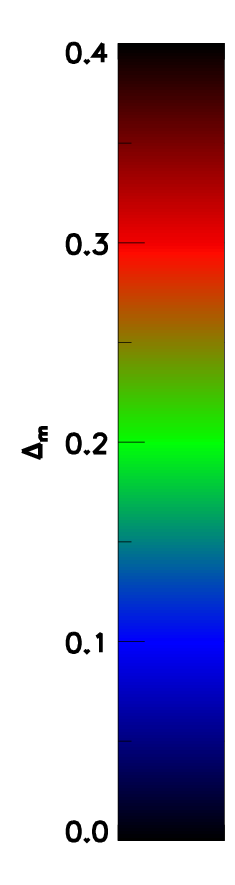
To test GR using dwarf galaxies, one of the first steps is to create a 3D screening map, which can be used to determine whether a galaxy is screened or not. In this section, using N-body simulation explained in the previous section, we develop a technique to find screened and unscreened galaxies. In the simulation we can estimate the degree of screening exactly by comparing the lensing mass and dynamical mass of the dark matter halos. We use , the difference between the dynamical and lensing mass, defined in Zhao et al (2011b), to quantify the degree of screening for the simulated halos. However, in our initial application to observational data we will use a binary classification, i.e. screened and unscreened.
In the gravity, the Poisson equation gets modified and reads,
| (2) |
where is Newton’s constant, is the gravitational potential (the time-time part in the perturbed FRW metric), is the perturbed Ricci scalar due to MG, and is the perturbed total effective energy density, which contains contributions from matter and modifications to the Einstein tensor due to MG. The dynamical mass of a halo is
| (3) |
where the integral is over the extension of the body. Physically, the dynamical mass means the mass inferred from the gravitational potential felt by a test particle at . Assuming the spherical symmetry, we can integrate the Poisson equation once to obtain
| (4) |
We actually use Eq. 4 to measure the dynamical masses of halos in our simulation. Note that if the gravity is modified, will be different from the lensing mass , the true mass of an object since includes the contribution from the scalar field, which mediates the finite-ranged fifth force within the Compton wavelength. Therefore, the relative difference ,
| (5) |
between the dynamical and lensing masses of the same object can be used as a indicator for MG.
From Eq. 4, we can estimate the range of by considering two extreme cases.
- (I)
-
In low density regions for unscreened galaxies, can be dropped, giving ;
- (II)
-
In high density regions where GR is locally restored, namely, , then .
So , which can be used to quantify the extent of the screening.
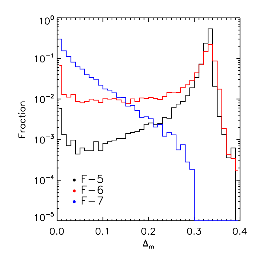
In Fig. 1 we show the degree of screening in different simulations. The figure shows the distribution of for simulations with different values. The fraction of unscreened galaxies (galaxies with higher ) is largest for the model – the fraction decreases with smaller values of . Some values of are higher than 1/3, due to numerical uncertainties.
3.2 Two Approximate Methods for Screening
We are interested in a sample of galaxies within a few hundred Mpc, especially low mass galaxies. Observations do not allow us to estimate lensing masses for these galaxies and thus estimate directly. This leads us to look for an alternate method to classify screened galaxies. We can estimate the dynamical masses of galaxies using measurements of luminosities or velocities. From the mass estimate we can find their virial radius under reasonable assumptions. Using the locations and dynamical masses of a reasonably complete galaxy catalog, we attempt to build a screening map using two simplified criteria as follows.
In gravity the chameleon effect recovers GR if , where is the Newtonian potential of the object (Hu & Sawicki 2007). This condition applies for an isolated spherical halo. We will make a simple approximation and use the same condition to determine whether an object is self-screened or environmentally screened. i.e. we look for the galaxies which satisfy the following conditions:
| (6) |
The first condition describes the self-screening condition. However, low-mass galaxies may be environmentally screened; the second condition is a simplified attempt at describing this, with being the Newtonial potential due to the neighbor galaxies within the background Compton length . for a galaxy is defined as
| (7) |
where the mass and the virial radius are related via . Here we use where is the critical density of the Universe. The external potential is evaluated using neighbors
| (8) |
where is the 3D distance to the neighboring galaxy with mass and virial radius , is the Compton wavelength and is the model parameter defined in Zhao et al (2011a, b).
The motivation for the above criteria is the following: the range of the fifth force is finite, defined by the Compton length . Our test galaxy will only feel the fifth force from neighbors within a distance of the -th galaxy (which itself must not be self-screened). We make the ansatz that the level of environmental screening is set by , though an accurate treatment requires a full solution of the scalar field equations. As we increase , the fifth force range becomes larger.
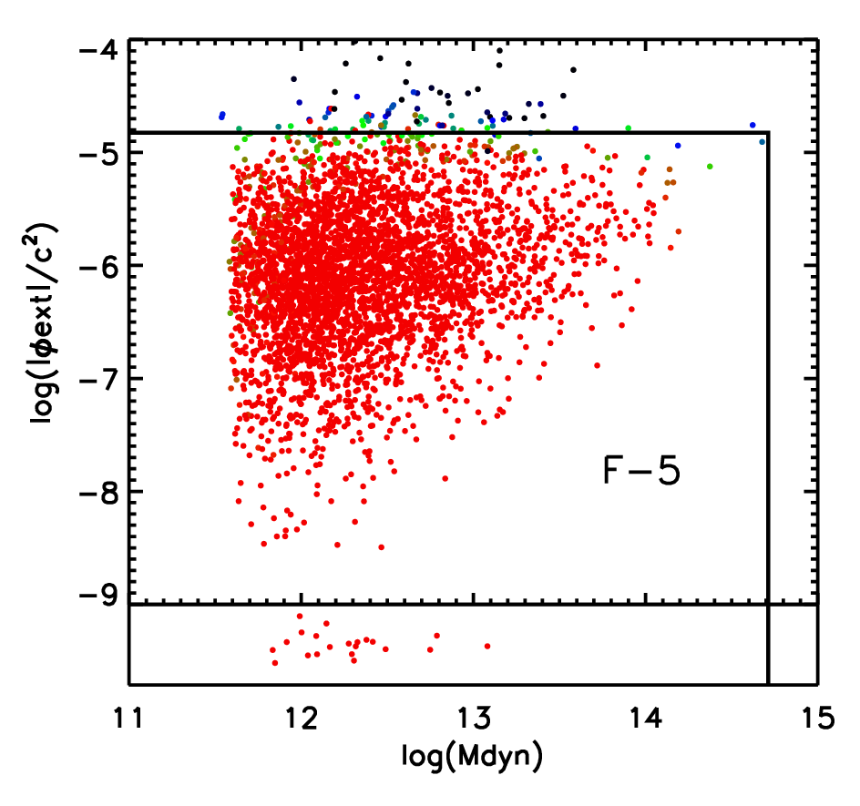
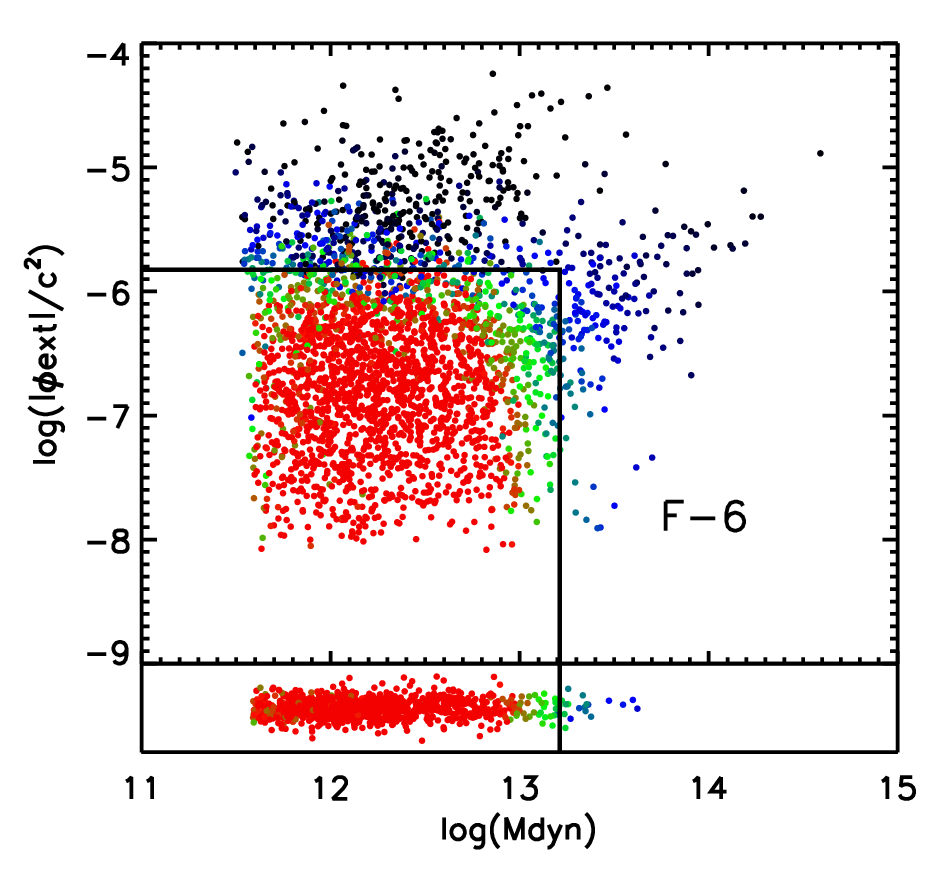
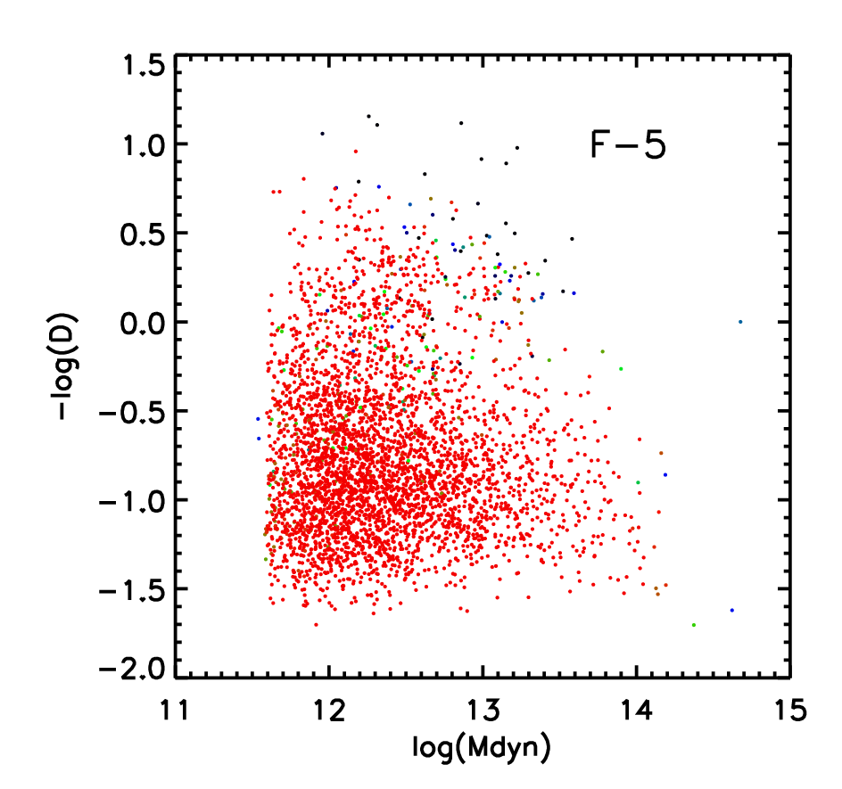
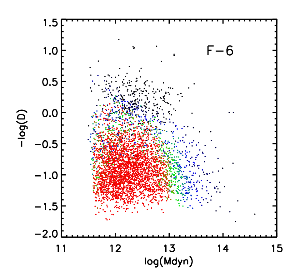
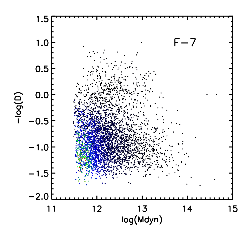
We use the N-body simulation described in the previous section to test the validity of the screening criteria of Eq. 6. We use dynamical mass from the simulation as it is the quantity that we can get easily from observations. The virial radius will also be obtained from . In Fig. 2 we show the screened and unscreened galaxies in the – plane. The points are colored according to the degree of screening (). The figure shows that we can classify objects as screened (blue) and unscreened (red) using simply defined boundaries set by . The minimum non-zero is given by galaxies with just one low-mass neighbor (limited by the simulation resolution of ) at a distance equal to . For the model the self-screening condition is satisfied for nearly all resolved halos. So we are not able to study the impact of environmental screening via the external potential for this model.
As an alternate criterion for environmental screening we study the parameter introduced by Haas et al (2011). For a test galaxy, it is defined in terms of its neighbors as:
| (9) |
where is the distance to the -th nearest neighbor with mass times higher than the test galaxy, and the virial radius of the neighbor galaxy. Previous studies, Haas et al (2011), show that (, hereafter) is a good estimator for environmental screening. The values of are set by the threshold on ; for the model, it is about 10 for a Milky Way sized galaxy with the threshold . See Fig. 3 for the distribution of in the - plane. Note how () and () are inversely correlated. However, the anti-correlation is not exact, since the weight in both estimators is different and uses information from multiple neighbors. From Fig. 2 and Fig. 3, we see that either or along with an estimate of is a good proxy for screening. The combination of both estimators does not provide significant extra information. We find below that the contamination is lower when using .
However, this simple analysis may have limitations when one uses real data. In order to evaluate the performance for survey data, we consider three cases below:
-
1.
The ideal case, i.e., without systematics. This allows us to study the intrinsic scatter around our cuts in or and .
-
2.
Consider the contamination due to each type of systematics one by one.
-
3.
Consider the realistic case, i.e., all three sources of uncertainties together.
3.3 Tests of Screening Without Systematic Errors
Using simulations we can learn how to separate screened/unscreened galaxies using observables. We will describe screening using cuts in , Eq. 6, or and (equivalent to ). We have considered more sophisticated classification methods but the systematics in the observables limit us to simple approximations at this time. We focus our study on the model, since the number of screened and unscreened galaxies is comparable there, and it is probably the most interesting case in terms of current limits. Towards the end, we will check how well our conclusions apply to other models.
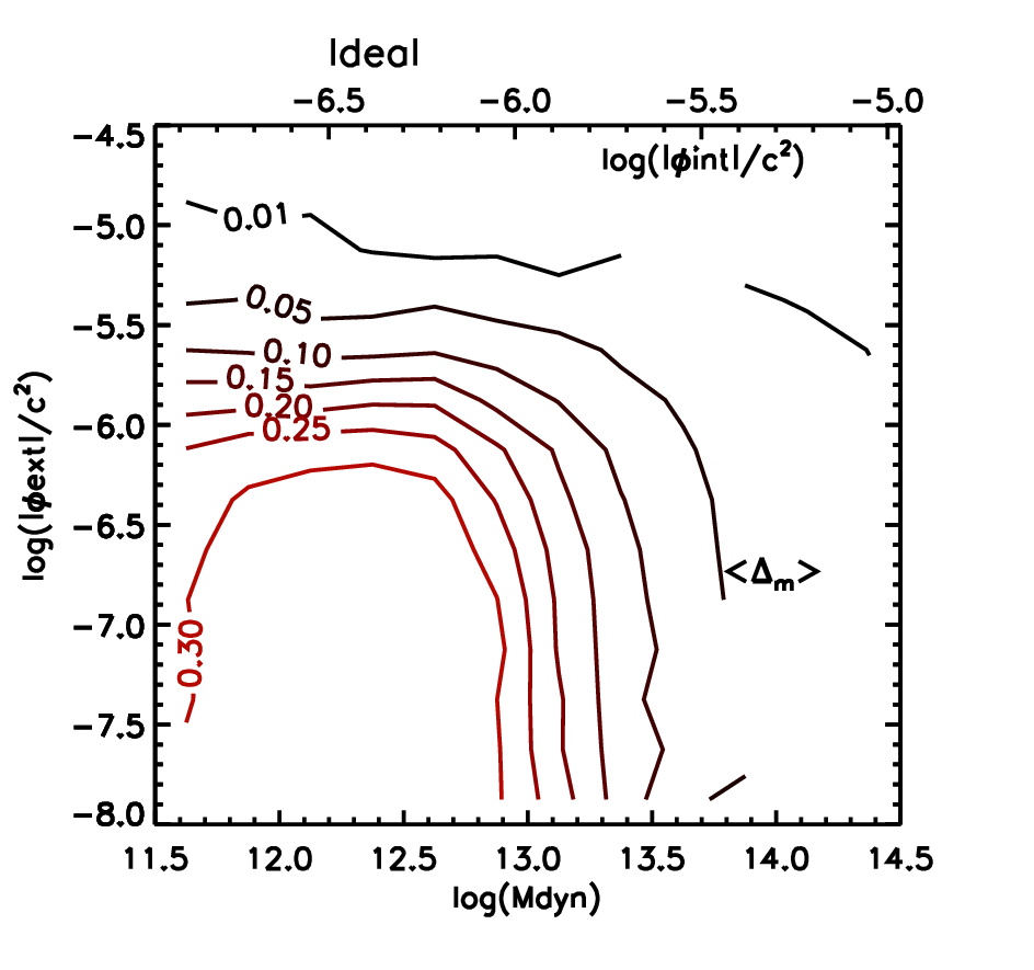
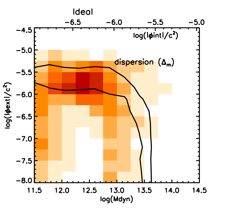
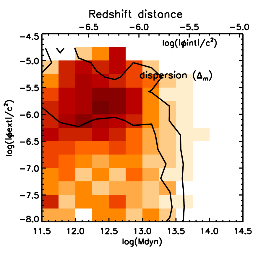
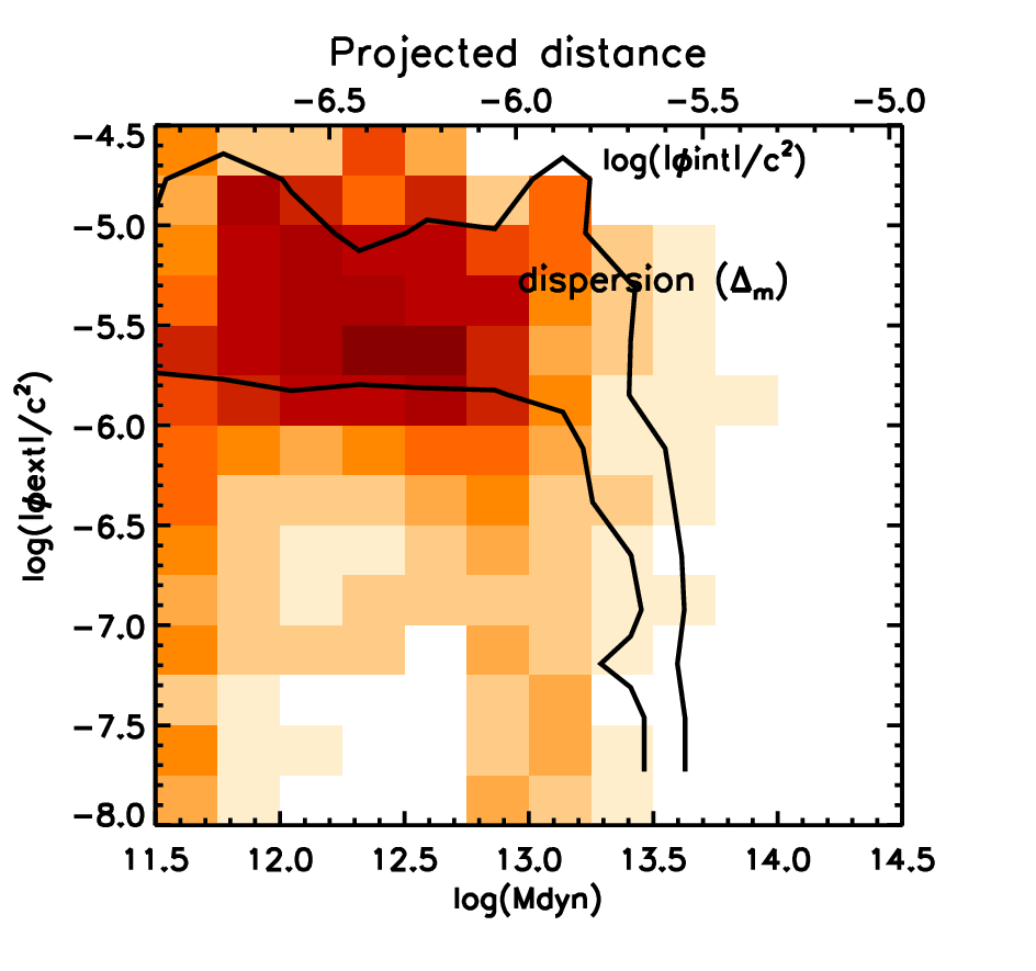
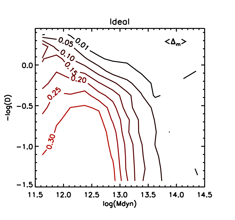
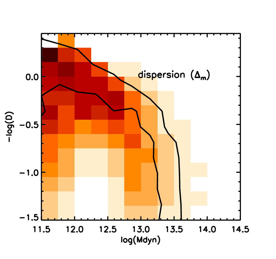
In Fig. 4 we show the contours of average in the – plane. We use bins of 0.25 in and . We can see that increases towards low mass halos in low density environments (smaller ). We see in the figure that it is possible to make a division between screened and unscreened halos based on a fiducial value of . It should also be noted that for any fiducial threshold value of the boundary looks mostly like a square defined by on the x-axis and on the y-axis. In this paper we set as the threshold value. Some part of the contamination evident in Fig. 2 comes from the dispersion of in the – plane. The top left panel of Fig. 5 shows this dispersion for the ideal case. It can be seen that the dispersion is larger () near the boundary defined by the environmental potential, where the classification is not so clean. We study below how this dispersion changes with different systematics. The overplotted contour lines in Fig. 5 demarcate 20% (lower line) and 80% (higher line) of screened galaxies (in each pixel).
At the end, the best cut will depend on the number of total galaxies. For the model , there are fewer screened galaxies than unscreened, hence the transition zone (where there is more contamination) will affect more the total contamination of screened galaxies. We go one step further and calculate the best cuts using the F-score test, a common algorithm used in machine learning in order to classify objects. This algorithm takes into account that both samples might have different number of galaxies and also minimizes the contamination in both directions. This can be done by maximizing the F-score estimator, which is defined as:
| (10) |
where is precision in screened galaxies and is recall, defined as follows. True positives (TP) are the screened galaxies that are tagged screened. False positives (FP) are the unscreened galaxies that are tagged screened. False negatives (FN) are the screened galaxies that are tagged unscreened. and are then defined as: and .
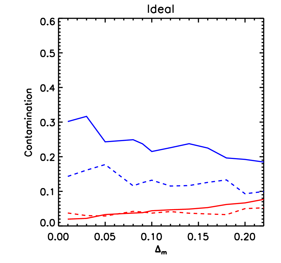
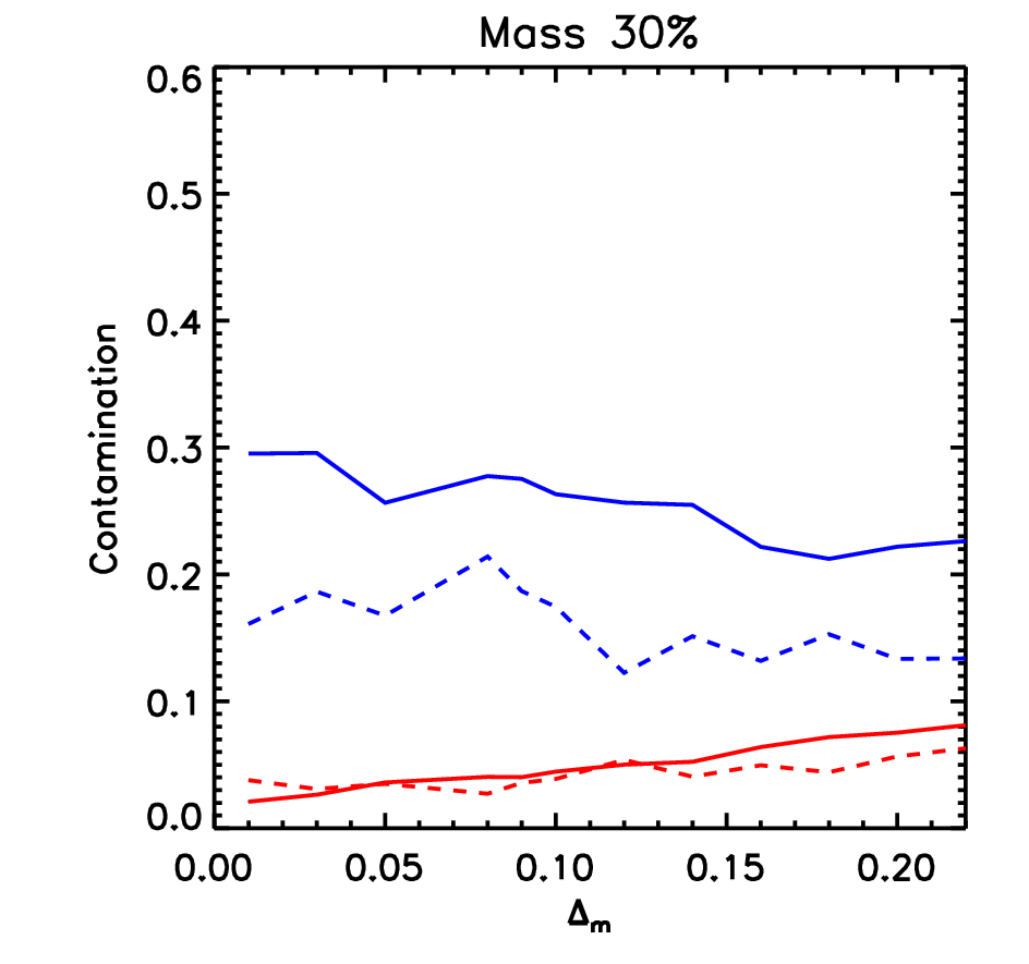
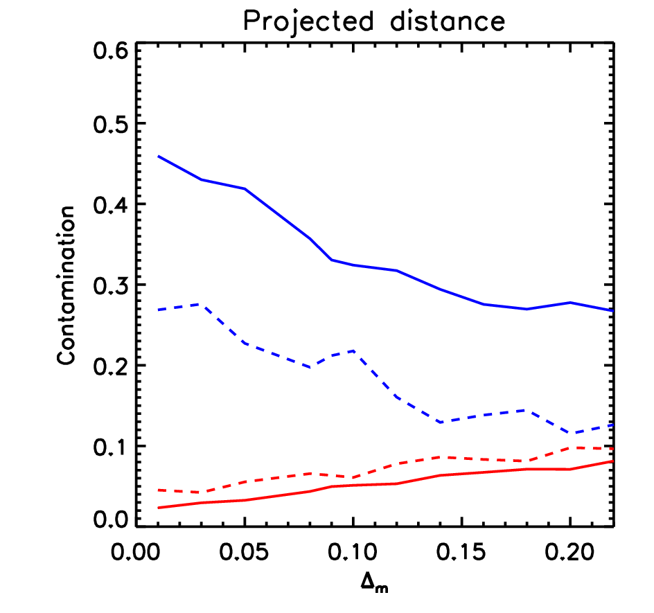
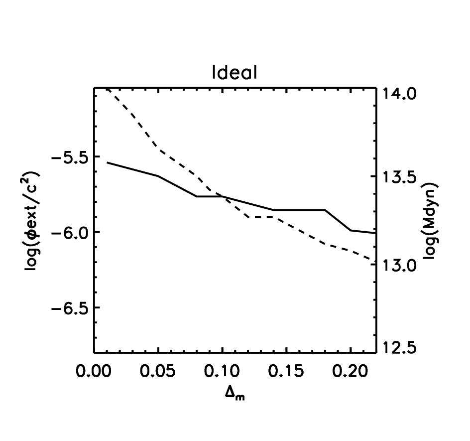
We plot the intrinsic contamination levels for screened (blue) and unscreened (red) galaxies for the - method (dashed) or the - method (solid) in Fig. 7 (top-left). The first method gives lower contamination for screened galaxies (blue) in the range 10-15% for . The contamination for unscreened galaxies is lower than 10% always, and consistent for both methods. In Fig. 8 we show the best cuts in (left axis, solid line) and (right axis, dashed line). The F-score is consistently around 0.8, which means that our suggested classification is robust.
We have performed the same analysis using - and we see in Fig. 6, top-left, that the cut is not as squared as in Fig. 4 so a sharp cut in and would not be accurate. This is the main reason why a cut in - does not work as good as - . In addition the dispersion, hence the contamination, is also higher. Note how contour plots in Fig. 4 give a cut in - similar to the one obtained when using the F-score (Fig. 8), which is a good consistency check.
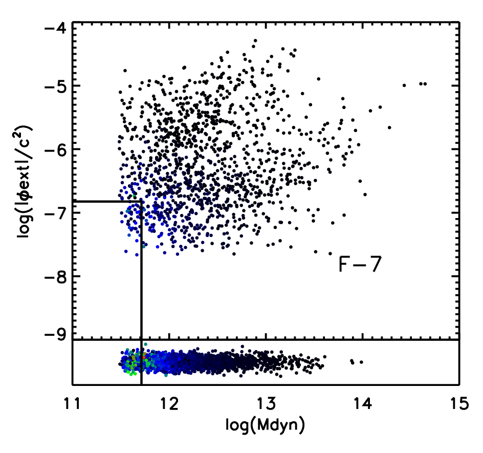
Now we extend our conclusions to other models. For , most of the galaxies are unscreened, only galaxies that reside near big clusters () will be screened. We see in Fig. 2 that the proposed cut is valid. As for , these simulations are not precise enough to study our proposed cut in detail, since we would need about one order of magnitude less massive galaxies to be confident of our tests.
3.4 Tests of Screening with Systematic Errors
In this section we study how systematic errors and other limitations in real surveys impact the screening methodology described above. There are three main sources of systematic errors in currently available data (in this paper we primarily use the SDSS galaxy catalog). These are:
-
1.
Uncertainty in mass estimate. For the current sample, the mass measurement is subject to 30% uncertainty.
-
2.
Uncertainty in the distance estimate. The distance measurement is subject to 3-10 Mpc/ (300-1000 km/s) uncertainty between galaxies in SDSS as the distances are derived from redshift measurements, which include peculiar velocities.
-
3.
Incompleteness. Somewhere between 5-20% of the neighboring galaxies for a typical test galaxy may be missing in our sample.
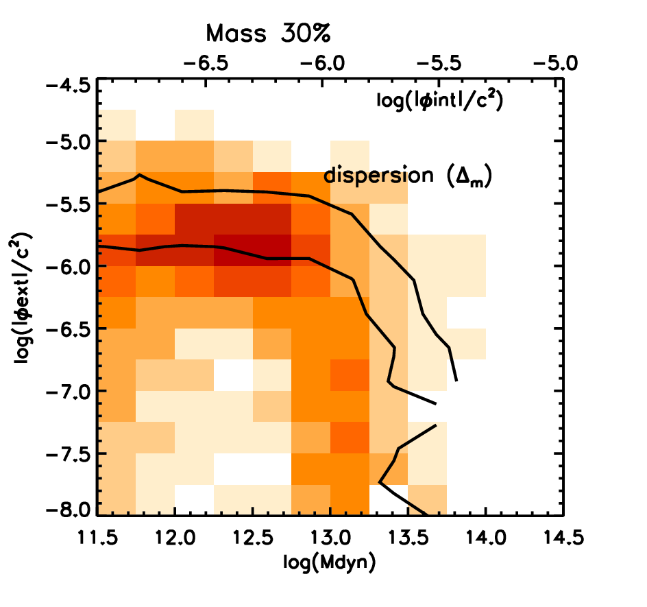
In order to study the uncertainty in galaxy halo mass, we add a 30% gaussian error to the dynamical mass in the simulations, both for test masses (the halo under classification) and neighbors. The virial radius is recalculated given the new estimated mass. See top-center plot in Fig. 5 and Fig. 7 to see the effect of mass uncertainty in the screening. The dispersion increases along the mass direction (Fig. 5). This implies that the contamination due to self-screening condition is larger than the contamination due to environmental screening condition. The best cuts in and are similar to the ideal case. However, the contamination increases up to 5% (for screened galaxies) with respect to the ideal case (Fig. 7).
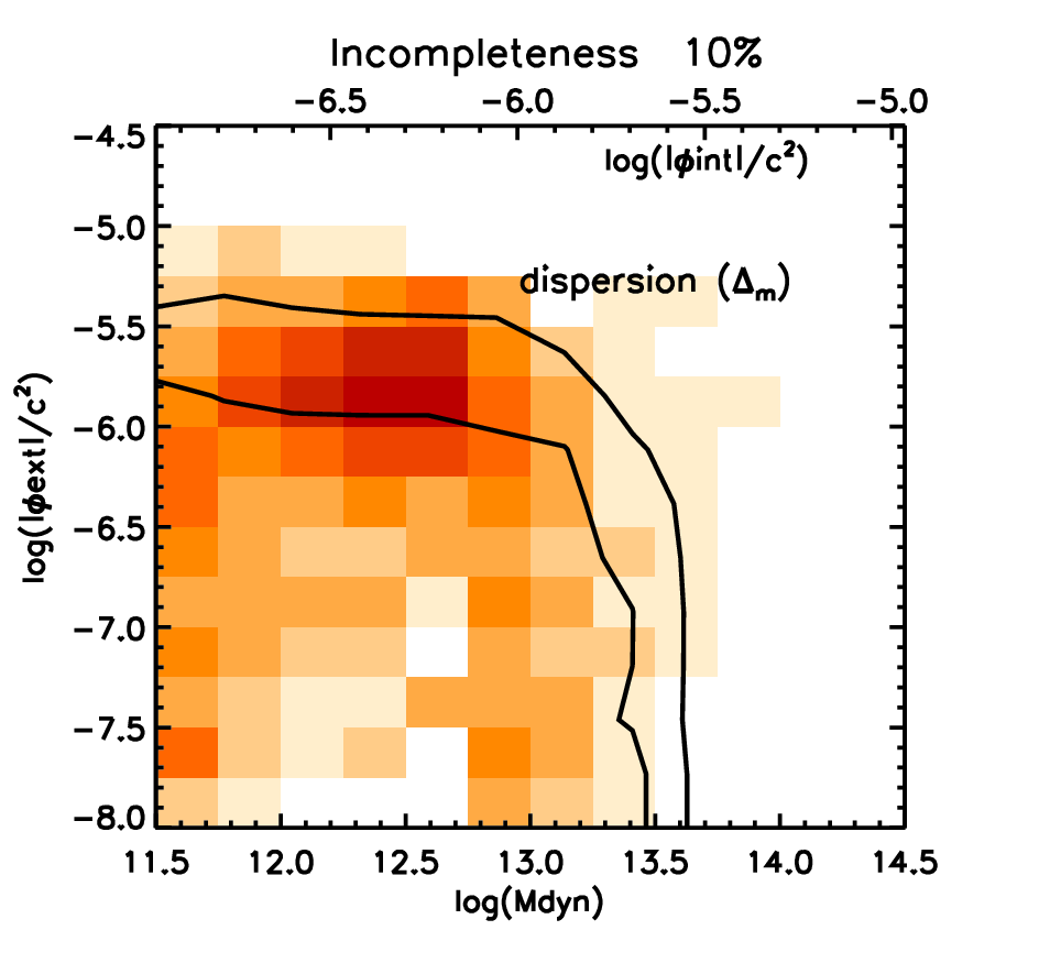
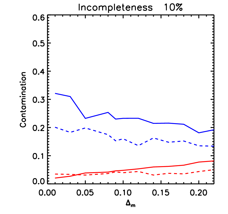
Next, we study the completeness in the catalog. The incompleteness can arise in survey catalogues due to masking or by edge effects. To mimic these effects we randomly reduce the number of neighbors by 10%. This incompleteness is independent of the mass. However, since there are more low mass galaxies in the universe, most of the randomly selected galaxies are low-mass. The effects due to incompleteness can be seen on the top-right plots (Fig. 5 and Fig. 7). In Fig. 5, we see that this systematic affects mainly low massive galaxies. The contamination in screened galaxies increases by around 5% (Fig. 7).
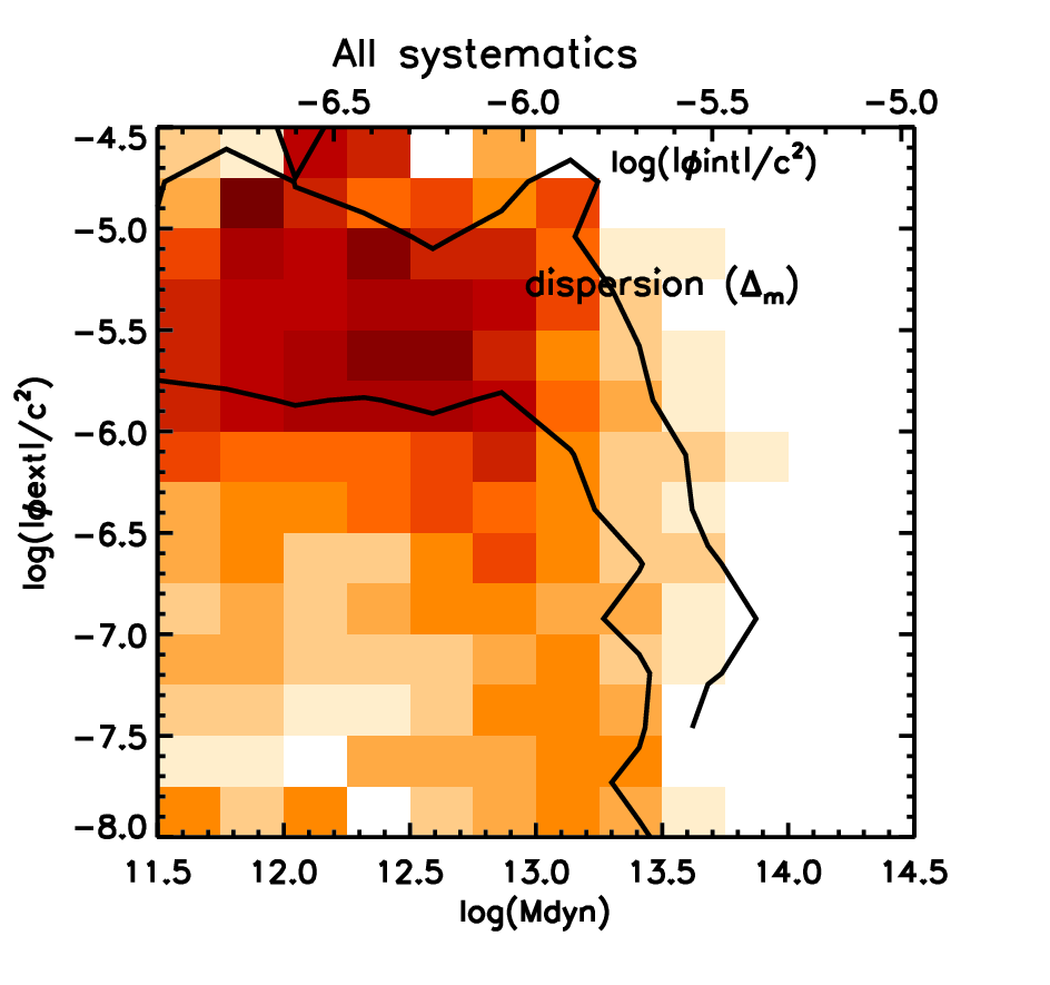
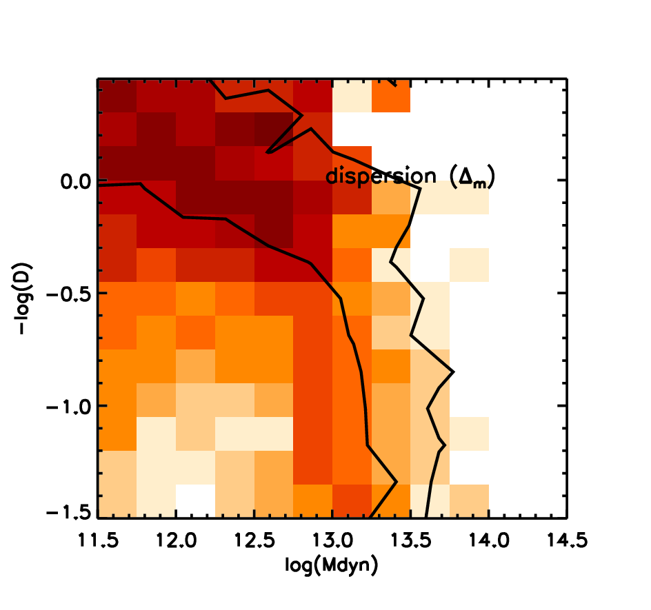
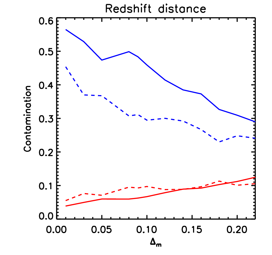
We also study the effect of uncertainties in distance on the classification. The distance uncertainty mainly originates from the use of redshift to estimate distances – which is affected by the peculiar velocities of the galaxies. In order to introduce this systematic in the simulation, we add the peculiar velocity distortion to the direction as . This systematic affects , since it changes the distance. It is a very large source of systematics as we can see in Fig. 5, bottom-left, and Fig. 7. We can reduce this systematic by estimating the distance using only the 2-D projected distance for suitably selected neighbors, and assuming spherical symmetry. We use neighbor galaxies within a line-of-sight distance of 5Mpc/h around the test galaxy (or equivalently 500km/s in the measured velocity). This is the velocity dispersion of an intermediate cluster. The improved results are on the bottom-center plot. We also checked the result using neighbors within a line-of-sight distance of 10 and 20 Mpc/h and found that the results remain the same. See bottom-left plot in Fig. 5 for a summary of all the systematics together.
We also tested what happens when there is incompleteness specifically in low mass neighbor galaxies used to determine . Not surprisingly we find that completeness is important for halo masses just below the self-screening threshold. We tested this with the simulations, and we expect that for the model this will be the principal limitation in our simulations.
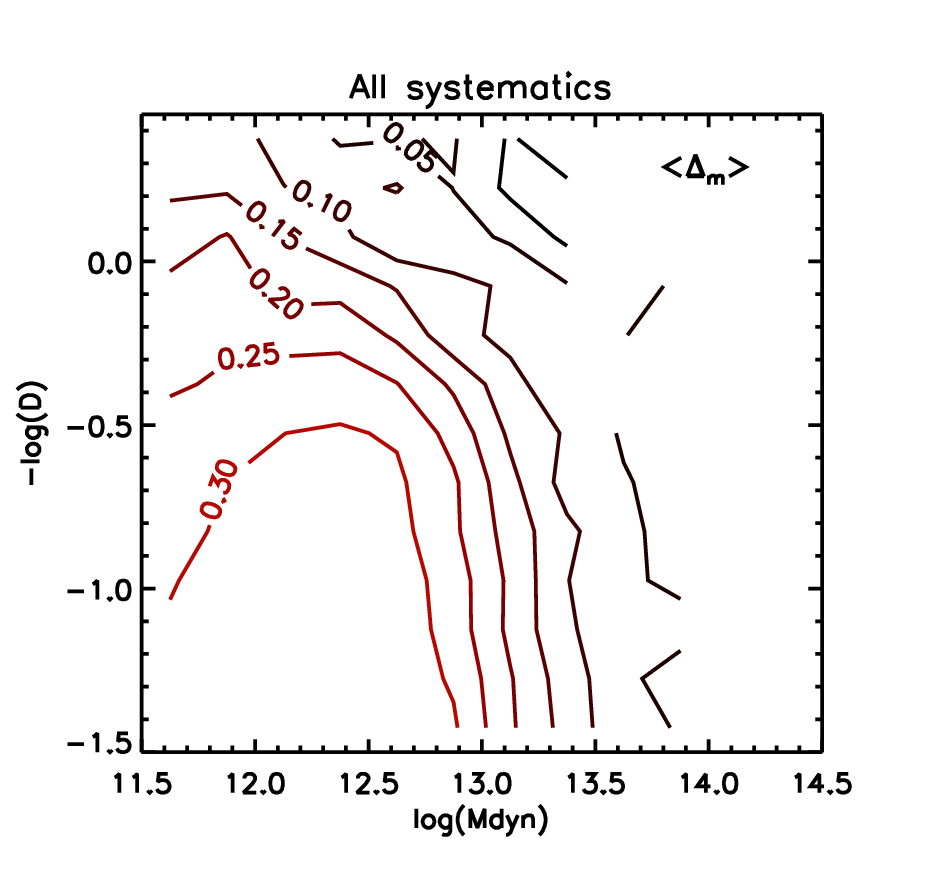
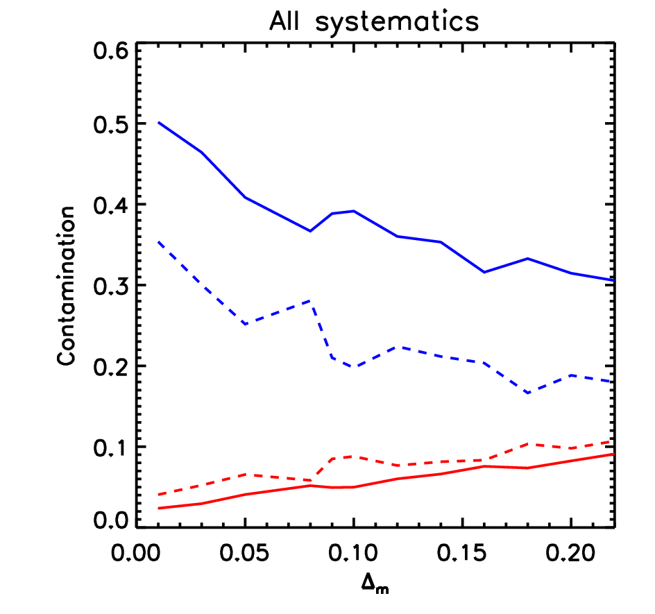
In conclusion, once we add systematics, the best cuts in and remain nearly the same as in the ideal case. However, the overall contamination nearly doubles compared to the ideal case. We did the same analysis for the second classification scheme based on -. The results are shown in Fig. 6. In the upper left panel we plot the contours of mean for the ideal case and in the upper right panel we show the contours with all systematics together. The bottom panels show the dispersion in for these two cases. We see that when adding the systematics the separator between screened and unscreened sample changes significantly from the ideal case. This makes these parameters harder to calibrate to reliably classify screened and unscreened galaxies. Also, the contamination is much larger than when using . Thus in the presence of systematics the – is preferred.
4 Screening Map for the SDSS Region
Tests of gravity with a sample of galaxies requires a screening map: given the coordinates of a test galaxy, such a map would allow one to determine the level of environmental screening. We have created a screening map over about 10,000 square degrees out to a distance of 210 Mpc using the SDSS group catalog created by Yang et al (2007) (DR7 version) and other surveys of galaxies and clusters.
The group catalog from the SDSS covers the redshift range 0.01-0.2 and includes close to 400,000 galaxies. We restrict our screening map to . Yang et al find group members using the friends-of-friends algorithm and calculate the group luminosity from member galaxies brighter than a certain threshold. The group luminosity is then converted to halo mass using an interative procedure that has been carefully tested with simulations. The mass of the groups ranges from to . They estimated the scatter in the estimated mass using mock catalogs and found that it is less than dex.
In the SDSS region, most of the contribution in our environmental screening map comes from the Yang et al (2007) groups, but we include other galaxy and cluster catalogs to determine 111NED provides a catalog of all the known extra galactic objects. We do not use this as many of the objects do not have absolute magnitudes which are required to estimate their masses. We do recommend supplementing the catalogs described here with NED-based data on neighboring galaxies for tests with a small enough sample of galaxies (so that case by case inspection is feasible). . We use the group catalog from 2M++ all sky survey (Lavaux and Hudson, 2011). There are 3984 2M++ groups of galaxies in our catalog. For local galaxies within 10 Mpc we use the galaxy catalog of Karachentsev et al (2004). These two catalogs improve our completeness for lower mass halos but not uniformly with distance.
We compiled a catalog of clusters with known redshifts using archival data. Our catalog mainly consists of Abell (Abell, Corwin and Olowin, 1989) and ROSAT (Ebeling et al, 1996) bright clusters. We ignore many clusters from the Abell catalog as they lack spectroscopic redshifts or lie beyond . Our catalog has a total of 675 clusters of galaxies.
A direct estimate of the masses of clusters and groups of galaxies can be found either by X-ray observation or by lensing observations. However, many of our clusters and groups do not have such an estimate. So we used established scaling relations to estimate the mass of clusters and groups. We use either the mass-luminosity relation given by Reiprich and Böhringer (2002) or the mass-velocity dispersion relation given by Evrard et al (2008) to determine the mass. For the galaxies within 10 Mpc we use the mass estimates given by Karachentsev et al (2004), which covers 313 out of 451 galaxies.
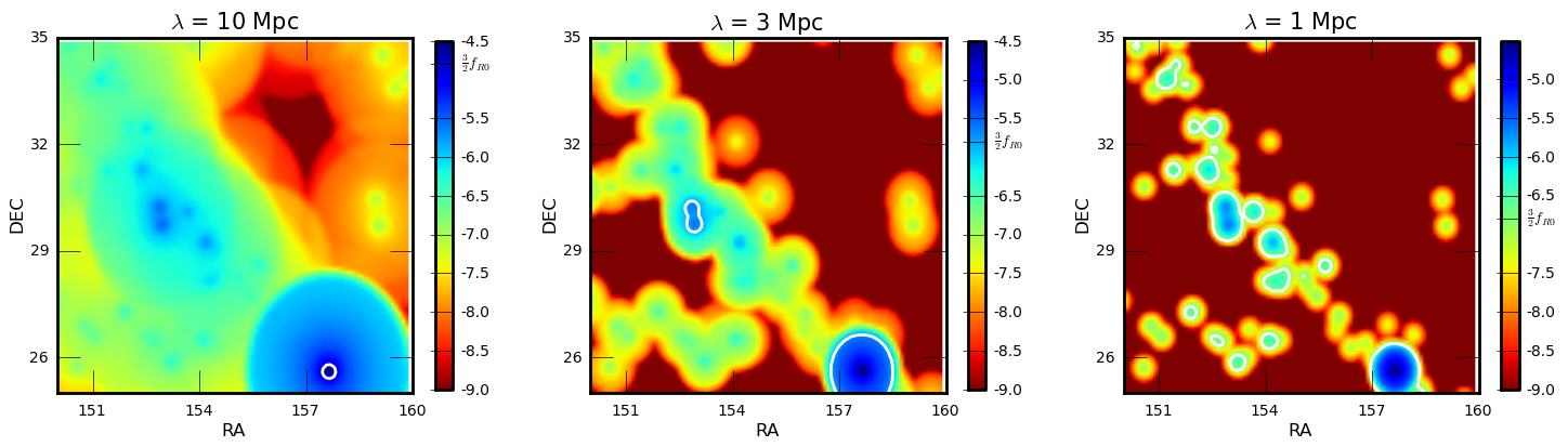
We chose a volume that extends to redshift , which is at a comoving distance of 210 Mpc and has an angular size of 10,000 square degrees. A 10 10 degrees (38 38 Mpc) patch of our map is shown in Fig. 9. The map is generated for different values of background Compton length (1 to 10 Mpc); each one corresponds to models with different parameter. Fig. 9 shows the result for the and models. Almost the entire volume is unscreened under a model – with the exception of massive and rare galaxy clusters, deep enough potential wells do not exist. While most of the volume also appears unscreened in the and models, galaxies reside preferentially in or near the screened regions so one has to be careful – for a specific galaxy sample, the fraction of screened galaxies depends on their mass distribution since the locations of galaxies (field vs. group) correlate with mass. The screening map and catalogs we make available allow one to determine the screening level for a galaxy at any location within the volume covered.
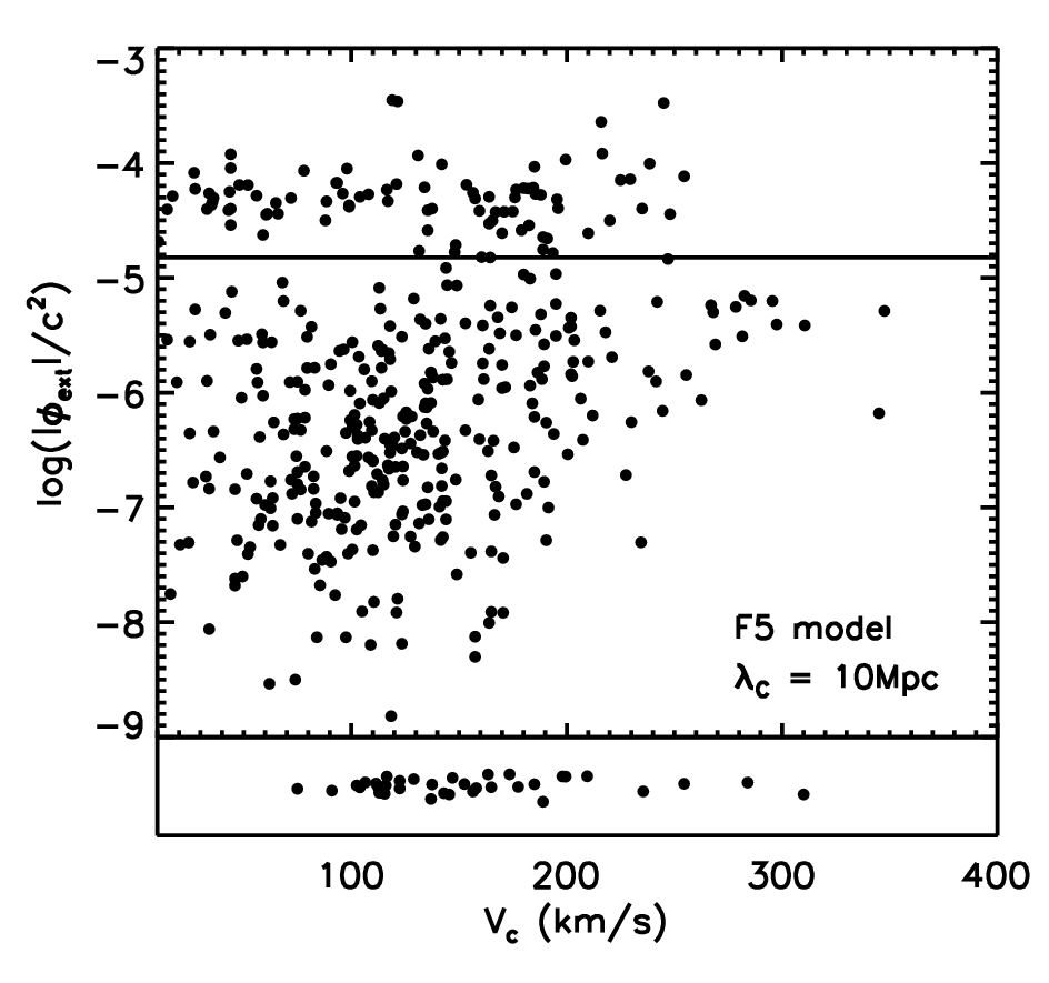
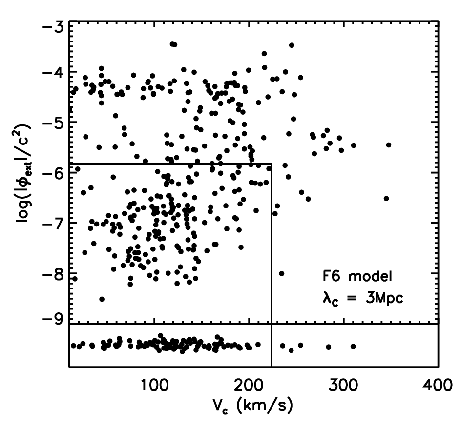
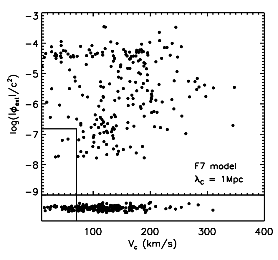
As an example, we study the scatter in for a set of nearly edge-on, rotationally supported galaxies selected to study warps as a probe for modified gravity following Jain and VanderPlas (2011). The details of the test will be presented elsewhere. These galaxies are selected inside the SDSS footprint. In Fig. 8 we plot for these galaxies for models (left), (middle) and (right). The peak circular velocity is used a proxy for . We overplot the limits for unscreened/screened following Eq. 6 using the conversion
| (11) |
Note how Fig. 10 and Fig. 2 are similar in range since the halo mass limit is similar in data and simulations (). In the model, we suffer from the small number of screened galaxies, but the classification should still be accurate. The model is the most complete while the model is likely to have incompleteness issues at larger distances.
For care must be exercised in using our map. Over the full 200 Mpc line of sight distance we do not have completeness for galaxies with halo mass below . Within 10 Mpc we do have information on galaxies with masses well below this limit. At distances beyond that, the mass limit of the combined dataset we have used must be evaluated with care. In particular, the catalogs described above are incomplete over the distance range 10-50 Mpc where the SDSS galaxy catalog should be used directly. In the tests we have carried out, we supplemented the catalogs described here with NED-based investigations of galaxy neighbors.
5 Conclusions
In order to test modified gravity theories with screening mechanisms, we need a criterion to separate screened from unscreened galaxies that is applicable to galaxy catalogs. We have tested two simple criteria for chameleon theories with simulations of gravity. While the criteria use simplified approximations to test for screening, we find they are successful at obtaining screened and unscreened subsamples that are robust to systematics.
For the criterion based on estimation of the external Newtonian potential, given in Eq. 6, we find that the intrinsic contamination is around 10%. We model the main expected systematics – mass uncertainty, incompleteness, and distance errors – and study how the contamination in the method degrades. For pessimistic assumptions, the contamination increases to about 20%. We are able to test the models and with catalogs from simulations. Our tests of the model are limited by the mass resolution of our simulations but we expect the criteria to scale simply to any relevant value of the background fields.
We applied our method to a catalog of galaxies in the SDSS region and constructed a screening map. For three discrete choices of the background field value we have shown examples of screening maps and samples of screened and unscreened galaxies. We have used our screening results in two companion studies of gravity tests with cepheids and with late-type dwarf galaxies (Jain et al 2012; Vikram et al 2012). We have also made available our compilation of input catalogs and code to evaluate screening222http://www.sas.upenn.edu/~vinu/screening/.
There are several caveats and possible improvements for future work. We have used approximate screening criteria, but for a given mass distribution the scalar field equations can be solved numerically to obtain more accurate screening maps. The contamination in the presence of systematics can be tested and controlled by discarding galaxies that are expected to be partially screened. Further, for a given screening level the thin shell condition allows for a quantitative estimate of partial screening. Finally, while our results are tested only with simulations, extension to other chameleon theories and symmetron or environmental dilaton based screening are feasible – see e.g. the discussion in Jain et al (2012).
6 Acknowledgements
We are very grateful to Baojiu Li for allowing us to use the halo catalog for the F4, F5 and F6 models, and for his help on obtaining the catalog for the F7 model. We also thank Xiaohu Yang for sharing the SDSS DR7 group catalogs. We acknowledge helpful discussions with Lam Hui, Mike Jarvis and Fabian Schmidt. AC and BJ are partially supported by NSF grant AST-0908027. GBZ and KK are supported by STFC grant ST/H002774/1. KK is also supported by the ERC and Leverhulme trust.
References
- Abell, Corwin and Olowin (1989) G. O. Abell, Jr. H. G. Corwin and R. P. Olowin, ApJs, 70, 1-138 (1989)
- Brax et al (2010) P. Brax, C. van de Bruck, A. C. Davis and D. Shaw, Phys. Rev. D82, 063519 (2010)
- De Felice and Tsujikawa (2010) A. De Felice, S. Tsujikawa, Living Rev. Rel. 13, 3 (2010)
- Davis et al (2011) A. C. Davis, E. A. Lim, J. Sakstein and D. Shaw arXiv:1102.5278 [astro-ph.CO] (2011)
- Ebeling et al (1996) H. Ebeling, W. Voges, H. Bohringer, A. C. Edge, J. P. Huchra and U. G. Briel, MNRAS, 281, 799-829 (1996)
- Evrard et al (2008) A. E. Evrard et al, ApJ, 672, 122-137 (2008)
- Haas et al (2011) M. R. Haas, J. Schaye and A. Jeeson-Daniel, MNRAS, 419, 2133-2146 (2012)
- Hinterbichler and Khoury (2010) K. Hinterbichler and J. Khoury, Phys. Rev. Let., 104, 231301 (2010)
- Hu and Sawicki (2007) W. Hu, I. Sawicki, Phys. Rev. D76, 064004 (2007)
- Hui, Nicolis and Stubbs (2009) L. Hui, A. Nicolis, C. Stubbs, Phys. Rev. D80, 104002 (2009)
- Jain and Khoury (2010) B. Jain, J. Khoury, Annals Phys. 325, 1479-1516 (2010)
- Jain (2011) B. Jain, Royal Society of London Philosophical Transactions Series A, 369, 5081-5089 (2011)
- Jain and VanderPlas (2011) B. Jain and J. VanderPlas, JCAP, 10, 32 (2011)
- Jain, Vikram and Sakstein (2012) B. Jain, V. Vikram and J. Sakstein, to be submitted
- Karachentsev et al (2004) I. D. Karachentsev, V. E. Karachentseva, W. K. Huchtmeier and D. I. Makarov AJ, 127, 2031-2068 (2004)
- Khoury and Weltman (2004) J. Khoury and A. Weltman, Phys. Rev. D69, 044026 (2004)
- Lavaux and Hudson (2011) G. Lavaux and M. J. Hudson, MNRAS, 416, 2840-2856 (2011)
- Li and Barrow (2007) B. Li and J. D. Barrow, Phys. Rev. D75, 084010 (2007)
- Li and Zhao (2009) B. Li and H. Zhao, Phys. Rev. D80, 044027 (2009)
- Li and Zhao (2010) B. Li and H. Zhao, Phys. Rev. D81, 104047 (2010)
- Li and Barrow (2011) B. Li and J. D. Barrow, Phys. Rev. D83, 024007 (2011)
- Lombriser et al (2010) L. Lombriser, A. Slosar, U. Seljak and W. Hu, arXiv:1003.3009 [astro-ph.CO] (2010)
- Reiprich and Böhringer (2002) T. H. Reiprich and H. Böhringer, ApJ, 567, 716-740 (2002)
- Schmidt et al (2009) F. Schmidt, M. V. Lima, H. Oyaizu, W. Hu, Phys. Rev. D79, 083518 (2009)
- Schmidt, Vikhlinin and Hu (2009) F. Schmidt, A. Vikhlinin and W. Hu, Phys. Rev. D80, 8, 083505 (2009)
- Schmidt (2010) F. Schmidt, Phys. Rev. D81, 103002 (2010)
- Silvestri and Trodden (2009) A. Silvestri and M. J. Trodden, Rept. Prog. Phys., 72, 096901 (2009)
- Smith (2009) T. L. Smith, arXiv:0907.4829 [astro-ph.CO] (2009)
- Song and Koyama (2009) Y. -S. Song, K. Koyama, JCAP 0901, 048 (2009)
- Sotiriou and Faraoni (2010) T. P. Sotiriou, V. Faraoni, Rev. Mod. Phys. 82, 451-497 (2010)
- Starobinsky (2007) A. A. Starobinsky, Soviet Journal of Experimental and Theoretical Physics Letters, 86, 157-163 (2007)
- Vainshtein (1972) A. I. Vainshtein, Phys. Lett. B39, 393-394 (1972)
- Vikram et al (2012) V. Vikram, A. Cabré, B. Jain and J. VanderPlas, in preparation.
- Will (2006) C. M. Will, Living Reviews in Relativity, 9, 3 (2006)
- Yang et al (2005) X. Yang, H. J. Mo, F. C. van den Bosch and Y. P. Jing MNRAS, 256, 1293 (2005)
- Yang et al (2007) X. Yang, H. J. Mo, F. C. van den Bosch, A. Pasquali, C. Li and M. Barden ApJ, 671, 153 (2007)
- Zhao et al (2011a) G. B. Zhao, B. Li and K. Koyama, Phys. Rev. D83, 044007 (2011a)
- Zhao et al (2011b) G. B. Zhao, B. Li and K. Koyama, Phys. Rev. Lett. 107, 071303 (2011b)