The Resolved Stellar Population in 50 Regions of M83 from HST/WFC3 Early Release Science Observations

Abstract

We present a multi-wavelength photometric study of $\sim$15,000 resolved stars in the nearby spiral galaxy M83 (NGC 5236, $D$ $=$ $4.61$ Mpc) based on $Hubble$ $Space$ $Telescope$ Wide Field Camera 3 observations using four filters: F336W, F438W, F555W, and F814W. We select 50 regions (an average size of 260 pc by 280 pc) in the spiral arm and inter-arm areas of M83, and determine the age distribution of the luminous stellar populations in each region. This is accomplished by correcting for extinction towards each individual star by comparing its colors with predictions from stellar isochrones. We compare the resulting luminosity weighted mean ages of the luminous stars in the 50 regions with those determined from several independent methods, including the number ratio of red-to-blue supergiants, morphological appearance of the regions, surface brightness fluctuations, and the ages of clusters in the regions. We find reasonably good agreement between these methods. We also find that young stars are much more likely to be found in concentrated aggregates along spiral arms, while older stars are more dispersed. These results are consistent with the scenario that star formation is associated with the spiral arms, and stars form primarily in star clusters and then disperse on short timescales to form the field population. The locations of Wolf-Rayet stars are found to correlate with the positions of many of the youngest regions, providing additional support for our ability to accurately estimate ages. We address the effects of spatial resolution on the measured colors, magnitudes, and age estimates. While individual stars can occasionally show measurable differences in the colors and magnitudes, the age estimates for entire regions are only slightly affected.

1. Introduction

Understanding the properties of stars and the history of star formation in galaxies remains one of the most fundamental subjects in astrophysics. The Hubble Space Telescope ($HST$) provides an important tool for this endeavor, since it enables the detailed study of stars and star clusters, not only in the Milky Way and its nearest neighbors, but in galaxies well beyond the Local Group. The Wide Field Camera 3 (WFC3) provides a particularly valuable new panchromatic imaging capability, with spectral coverage from the near-UV to the near-IR. This capability is especially useful for studying the stellar populations in nearby galaxies where individual stars are resolved.

A good example of a multi-wavelength survey of nearby galaxies which employs resolved stars and star clusters is the ACS Nearby Galaxy Treasury (ANGST) program (Dalcanton et al., 2009). This study includes $\sim$65 galaxies out to $\sim$3.5 Mpc, and provides uniform multi-color ($BVI$) catalogs of tens of thousands of individual stars in each galaxy. Although the ANGST program provides an excellent survey for a wide range of studies, it does not provide observations in the $U$-band since the observations were obtained before WFC3 was installed on $HST$. The $U$-band is particularly useful for age-dating populations of young stars, which is the focus of the current paper. PHAT (Panchromatic Hubble Andromeda Treasury) is a related study that does take advantage of the new $U$-band capability on WFC3. While nowhere as extensive as the Multiple Cycle Treasury Program PHAT survey, the current study of M83 is complementary in the sense that it provides similar observations of the resolved stellar component of a nearby spiral galaxy, and uses quite different analysis techniques, as will be discussed in Sections 2 and 3. Future observations of M83 (ID:12513, PI: William Blair) will expand the WFC3 dataset available for M83 from 2 to 7 fields.

M83 (NGC 5236), also known as the “Southern Pinwheel” galaxy, is a slightly barred spiral galaxy with a starbursting nucleus located at a distance of $4.61$ Mpc, i.e., $(m-M)_{0}=28.32\pm 0.13$ (Saha et al., 2006). The H$\alpha$ emission can be used to pinpoint regions of recently formed massive stars along the spiral arms, while red supergiants can be found throughout the galaxy. The color-magnitude diagram (CMD) of resolved stars is a powerful diagnostic tool for understanding the stellar evolution and history of star formation of galaxies in detail. By comparing stellar evolution models to observed CMDs, we are able to determine the ages of the stellar populations in galaxies. However, in active star-forming regions, the stars are often partially obscured by dust. Applying a single extinction correction value for the whole galaxy often results in over- or under-estimates of the ages of individual stars. If the CMD is the only tool used to determine the ages, the spatial variations of dust extinction in galaxies and their effects on the determined ages are not readily apparent. The additional information available from the color-color diagram can remedy this problem. By using techniques developed in this paper, we can constrain the variations of dust extinction across M83, and make corrections for individual stars. We also focus on spatial variations in the stellar properties throughout the galaxy.

The $HST$ WFC3 observations of M83 were performed in August 2009 as part of the WFC3 Science Oversight Committee (SOC) Early Release Science (ERS) program (ID:11360, PI: Robert O’Connell). The central region (3.2 kpc$\times$3.2 kpc) of M83 was observed in August, 2009. A second adjacent field to the NNW was observed in March 2010, and will be included in future publications. Details of the WFC3 ERS data calibration and processing are given by Chandar et al. (2010) and Windhorst et al. (2011).

In this paper we present $UBVI$ photometry of resolved stars in M83 and the resulting color-color and color-magnitude diagrams. We use $(F336W\!-\!F438W)$ vs. $(F555W\!-\!F814W)$ color-color diagrams to constrain the variation of dust extinction along the line-of-sight of each individual star, and correct $F814W$ vs. $(F555W\!-\!F814W)$ CMDs for the extinction of individual stars to determine their ages. The high sensitivity and the superb resolving power in the WFC3 F336W-band plays a key role in allowing us to develop our extinction correction techniques, and demonstrate the performance of the newly installed WFC3. This results in improved stellar age estimates, and a better understanding of the recent star-formation history of M83.

Our investigations are focused on the followings:

1. Do we see spatial variations of stellar ages in M83? If so, can we use these variations to learn more about the evolution of the galaxy and what triggers star formation?

2. How well do various age estimates correlate (i.e., resolved stars, integrated light, clusters, number ratio of red-to-blue stars, H$\alpha$ morphology, stellar surface brightness fluctuations, presence of Wolf-Rayet stars)?

This paper is organized as follows. In §2, we describe the observations, photometric analysis, and the extinction correction method. CMDs and color-color diagrams of the 50 selected regions are then used to provide stellar age estimates, as described in §3. Comparisons with other age estimates (i.e., integrated light and star clusters) are also made. In §4, we compare the stellar ages to a variety of other parameters that correlate with age, including red-to-blue star ratios, $H\alpha$ morphology, and surface brightness fluctuations. Section 5 includes a discussion of how these comparisons can be used as diagnostics, with special attention paid to the question of what spatial variations can tell us about the star formation history in M83, and on the question of how star clusters might dissolve and populate the field. A summary of our primary results is provided in §6. In Appendix A, we investigate the locations of sources of Wolf-Rayet stars in our M83 field and discuss the correlation with the positions of young regions. In Appendix B, we describe how the spatial resolution affects our measured colors and magnitudes, and our age estimates of stars in our M83 field.

2. HST WFC3 Observations

2.1. The WFC3/UVIS Data

The data were obtained in seven broad- and seven narrow-band filters in the WFC3 UVIS and IR channels. Details are described in Dopita et al. (2010) and Chandar et al. (2010). In the current paper we use four broad-band images. The filters and exposure times are F336W (1890 sec), F438W (1880 sec), F555W (1203 sec), and F814W (1203 sec). Although we do not make transformations to the Johnson-Kron-Cousins $UBVI$ system, we will refer to these filters as $U$, $B$, $V$, and $I$ for convenience. Three exposures were taken in each filter at different dithered positions to remove cosmic rays, the intrachip gap, and to partially compensate for the undersampled point-spread function (PSF) of the WFC3/UVIS channel. The raw data were processed using the MULTIDRIZZLE software (Koekemoer et al., 2002) with an effective pixel size of 0$\farcs$0396, which corresponds to 0.885 pc per pixel at the distance of 4.61 Mpc (Saha et al., 2006). The resulting multidrizzled images are combined, cosmic-ray removed, and distortion-corrected. A color composite of the F336W, F555W, F814W (broad bands) and F502N, F657N (narrow bands) images is shown in Figure 1. It covers the nuclear region of M83, part of its eastern spiral arm, and the inter-arm region. Stars in the cores of compact star clusters are not resolved at this resolution, but the brighter stars in the outskirts of the star clusters and in the field are generally resolved into individual stars. Details of the effects of spatial resolution are discussed in Appendix B. Since we are interested in spatial variations of stellar ages in M83, we selected 50 regions in the spiral arm and inter-arm areas. Boxes outlined in blue (very young – age $\lesssim$ 10 Myr, see §3), yellow (young – 10 $\lesssim$ age $\lesssim$ 20 Myr), and red (intermediate-aged – age $\gtrsim$ 20 Myr) in Figure 1 show the 50 regions selected for detailed study in this paper.

2.2. Photometry and Artificial Star Tests

Photometric analysis of the WFC3 M83 data was performed on the $U$, $B$, $V$, and $I$ images using the DoPHOT package (Schechter et al., 1993) with modifications made by A. Saha. Additional routines to derive parameters for the kurtosis of the analytic PSFs used by DoPHOT, and for post-processing DoPHOT output to obtain calibrated aperture-corrected photometry, were performed using customized IDL code written by Saha. A more detailed description of these procedures can be found in Saha et al. (2010). The kurtosis terms were derived by fitting the functional form of the DoPHOT analytic PSF to 20 relatively bright and isolated stars. The remaining shape parameters ($\sigma_{x}$, $\sigma_{y}$, and $\sigma_{xy}$) are dynamically optimized within DoPHOT.

The difference between the shape parameters for an individual object and those for a typical star was calculated and used to classify the object as a star, a galaxy, or a double-star. The shape parameters were determined separately for each image. The numbers of objects classified as stars are approximately 20,000 in $U$ and $B$, 17,000 in $V$, and 15,000 in $I$ band images, respectively. The calculated Full Width at Half Maximum (FWHMs) are $U$ = 0$\farcs$096 (2.42 pixel), $B$ = 0$\farcs$093 (2.34 pixel), $V$ = 0$\farcs$091 (2.29 pixel), and $I$ = 0$\farcs$113 (2.85 pixel). All magnitudes are in the WFC3-UVIS VEGAMAG magnitude system, calculated using equation (4) in Sirianni et al. (2005) and the latest zeropoint magnitudes: $U$ = 23.46, $B$ = 24.98, $V$ = 25.81, and $I$ = 24.67 mag, provided by STScI at the $HST$/WFC3 website.

A multi-wavelength $UBVI$ catalog was then constructed by matching the individual objects in each catalog between these filters. Interestingly, we found that the extreme image crowding in these images, combined with the excellent panchromatic sensitivity and unprecedented spatial resolution provided by the newly installed WFC3, introduced a new challenge during this matching step, with large numbers of “pseudo” matches occurring if too-large a match radius was used. We discuss the effects of spatial resolution in Appendix B.

Figure 2 demonstrates this problem by showing the $F555W$ and color composite image cut-outs near Regions # 26 and # 27. In the middle panel of Figure 2, stars circled in red are objects with $(V\!-\!I)$ colors that are very red ($(V-I)>1.2$ mag), but have $(U\!-\!B)$ values that are fairly blue ($-0.4<(U-B)<-1.7$ mag). These can be seen as the spray of points in the upper right parts of the top right panels of Figures 3 and 4, which will be discussed below. As shown by the postage stamp images in Figure 2, about half of these are likely to be blue stars with very high values of reddening (i.e., the bottom panel and the small postage stamps on the right show that they are in dusty regions), while the other half are very close superpositions of at least one red and one blue star, which we will call “pseudo” matches (i.e., the panels on the left show a strong blue and red gradient across many of the objects).

We found that using a very small matching radius of 0.5 pixels was needed to minimize “pseudo” matches in our catalog. Earlier attempts using a matching radius of 3 pixels resulted in $\sim$10 % pseudo matches. Accurate matching also requires precise geometric distortion corrections in all filters. However, even when these conditions are met, there is a finite chance that two different stars will fall within the same aperture. This is most easily seen by blinking the $U$- and $I$-band images. While the single stars stay in the same position, the pseudo match stars move slightly, showing they are two different stars with different colors.

The final stellar catalog contains $\sim$15,000 objects. We find that our procedure results in only a few percent of pseudo matches, as will be discussed in §2.4 (i.e., the upper right panel of Figure 4).

To measure the photometric completeness, we performed artificial star tests with the same detection and photometry procedure as applied to the actual stars. We inserted 1000 artificial stars with Gaussian PSFs and FWHMs appropriate for these stars at random positions into all four images. The magnitude of the inserted stars varied from 22 to 28 mag in steps of 0.25 mag. The 50% completeness levels at 5 $\sigma$ detection thresholds for a typical region are reached at recovery magnitudes of approximately 24.3, 25.1, 25.3, and 24.8 mag for the $U$, $B$, $V$, and $I$ images, respectively. These limits can vary by about a magnitude, depending on the brightness of the background in a given region. The exception is Region # 48, which includes the nucleus. The completeness thresholds are two or more magnitudes brighter in this region due to the very high background. This region has therefore been excluded from the rest of the discussion, but is included in Table LABEL:tab:50reg for reference.

2.3. CMDs and Color-color Diagrams in M83

The top panels of Figure 3 show the $I$ vs. ($V-I$) CMD (left) and the $(U\!-\!B)$  vs. $(V\!-\!I)$  color-color diagram (right) of resolved stars extracted from the cross-matched catalog. The CMD shows the presence of young main-sequence (MS) stars, transition or He-burning “blue loop” stars, red giant stars (hydrogen shell-burning and hydrogen$+$helium shell-burning stars), and a relatively small number of low-mass red-giant branch (RGB) stars. This is because the tip of the low-mass RGB stars is at $I$ = 24.7 mag (Karachentsev et al., 2007), which is roughly the same as our completeness threshold. The ages of these stars range from $\approx$ 1 to $\approx$ 100 Myr. The Padova isochrones (Marigo et al., 2008) ranging in age from log $\tau$ (age/yr) = 6.55 (3.5 Myr) to log $\tau$ (age/yr) = 8.0 (100 Myr) are included in Figure 3 for reference. We note that the younger isochrones (e.g., 1 Myr) fall nearly on top of the 3.5  Myr isochrone, and hence are not included in the diagram.

The arrows in both panels show $A_{V}\!=\!1$ reddening vectors for M83 using the $R_{V}=3.1$ extinction curve of Cardelli et al. (1989). Corrections have been made for foreground Galactic extinction (Schlegel et al., 1998) using $A_{F336W}=0.361$, $A_{F438W}=0.290$, $A_{F555W}=0.229$, and $A_{F814W}=0.133$ mag, respectively. In Figure 3, we only plot stars with photometric errors less than 0.25 mag in the filters used for each diagram. The numbers of objects plotted in the CMD and the color-color diagram are about 12,000 and 8,500 stars, respectively. Since approximately 30% of the stars are not detected in one or more of the $U$, $B$, or $I$ filters, due to either reddening or intrinsically red or blue colors, fewer stars are plotted in the color-color diagram.

We adopt a value of 1.5 times solar metallicity (Z=0.03), the highest metallicity isochrones available from the Padova database, for M83 based on Bresolin & Kennicutt (2002). A test using solar metallicity (Z=0.019) isochrones showed that the ages for a typical region would be $\approx$ 2 Myr older if the lower metallicity is adopted. This agrees with the study by Larsen et al. (2011), who found that the simulated CMDs of young massive clusters in M83 with solar and super-solar metallicity isochrones would not look much different. Theoretical isochrones calculated for the WFC3 filters and Z=0.03 (1.5 Z_☉) from the Padova database (Marigo et al., 2008) are overlaid on both panels in Figure 3. The dashed line in cyan shows the 50% completeness level in $I$ and $(V\!-\!I)$, using the completeness threshold numbers from the artificial star test in §2.2.

The bottom panels of Figures 3 and 4 show the histograms of ages and masses for the same stars plotted in the CMD and color-color diagram. The ages and masses of stars were estimated by finding the closest match between the $I$ and $(V\!-\!I)$ values for each star, using a fine mesh of the stellar isochrones plotted in the CMD and color-color diagram in Figures 3 and 4. More details about the stellar age-dating from the CMDs and the stellar isochrones are given in §3.1.

2.4. Extinction Corrections

Since M83 has an intricate structure of dust lanes associated with active star forming regions in the spiral arms and thin layers of dust in the inter-arm area in Figure 1, we cannot use a single value of internal extinction and apply it to correct for the extinction of all stars in a given region. In the color-color diagram in Figure 3, we notice that while the bluest stars match the model isochrones quite well after we correct for Galactic foreground extinction, the majority of stars are found redward of the models, implying a typical extinction of $A_{V}\!\simeq\!0.5$ mag (for the densest part of the data “swarm”). As described below, we can determine the reddening of these stars if we assume that they are intrinsically blue stars that belong on the Padova models (i.e., with $(V-I)\simeq-0.3$ mag). A visual inspection supports this interpretation. Stars with observed values of $(V-I)\approx-0.3$ mag are found in areas with no obvious dust features surrounding them while stars with $(V-I)>0.5$ mag are near dust filaments.

Our basic approach to correct the colors (and luminosities) of individual stars for the effects of extinction is to backtrack the position along the reddening vector for each data point, until we hit the stellar isochrones in the color-color diagram. What makes this method work is the fact that all the isochrones are nearly on top of each other in the range $(U\!-\!B)\!<\!0.0$ mag. The way we apply this in practice is to match the observed and predicted values of the reddening free $Q$ parameter defined by:

$$Q_{UBVI}=(U-B)-\frac{E(U-B)}{E(V-I)}\times(V-I)$$ (1)

(Mihalas & Binney, 1981). Using observed values of $UBVI$, we compute the observed $Q_{UBVI}$ values by using the standard slope of $E(U\!-\!B)/E(V\!-\!I)=0.58$ (Mihalas & Binney, 1981; Whitmore et al., 1999), which corresponds to $R_{V}=3.1$. The predicted $Q$ values are calculated using the 1.5 Z_⊙ Padova isochrones. A complication is that we cannot simply use the matched $Q$ values to determine corrected values of $(U\!-\!B)$ and $(V\!-\!I)$, since they would, by definition, fall precisely on the isochrones (i.e., we would be using circular reasoning). Instead, we solve for the extinction in $(U\!-\!I)$, which is partly independent and uses the longest wavelength baseline. We then calculate the extinction values in $UBVI$ and the color excess values in $(U\!-\!B)$ and $(V\!-\!I)$. The averages of the corrected internal extinction and color excess values by our star-by-star correction method are $A_{F336W}=$ 0.696, $A_{F438W}=$ 0.559, $A_{F555W}=$ 0.441, $A_{F814W}=$ 0.256 mag, and $E(U\!-\!B)=$ 0.137 and $E(V\!-\!I)=$ 0.185 mag. This is similar to the average internal extinction ($A_{F555W}=0.425$ mag) estimated from the cluster SED fitting by Bastian et al. (2011). However, our results differ from the average extinction ($A_{V}=0.671$ mag) of 45 clusters in the nucleus ($\sim 20\arcsec$ in diameter) of M83, determined from $H\alpha/H\beta$ ratios by Harris et al. (2001). This is consistent with the finding of larger extinction in the nuclear region by Chandar et al. (2010).

In the color-color diagram (top right panel) of Figure 3, we note that while most of the data points are consistent with the standard reddening vector, the stars located in the green triangle appear to follow a flatter reddening vector. Whether this is actually due to a different reddening law in M83 (e.g., as has been suggested for heavily extincted regions such as # 4, # 12, and # 20), or is some sort of artifact (e.g. due to photometric uncertainties, unresolved star clusters, or the “pseudo” matching problem discussed above) is difficult to determine from our present dataset. However, for our specific needs the precise answer to this question is not critical. Our approach will be to correct the data points in the triangle back to a position near the top of the isochrones, as shown by the intersection of the red dotted line and the isochrones in Figure 4. This is equivalent to using a range in $R_{V}$ between 3.1 and 5.7 (the value represented by the red dotted line).

The upper panels of Figure 4 show the CMD and color-color diagram corrected for the internal extinction in M83. The arrows in both panels are the reddening vectors. We do not apply an extinction correction for stars with $(V-I)\geq 1.2$ mag, or above an extrapolation of the flatter extinction vector from the bluest possible isochrones (see the red dotted lines in the upper right panel of Figure 4), since we believe that the colors of many of these sources are incorrect (i.e., roughly half are likely to be pseudo matches, as discussed in §2.2 and shown in Figure 2). We note that only about 4 % of the stars fall in this part of the diagram. These stars are removed from the subsequent analysis. If we include these stars, our age estimates typically increase by about 1 Myr.

Also, stars below the blue dotted line in Figure 4 are not corrected for extinction, since these are main sequence turnoff stars (i.e., blue loop or transition stars in general), and hence, do not have unique $UBVI$ colors for the stars along a given reddening line, unlike the main sequence stars with $(U\!-\!B)\!<\!0.0$ mag.

Based on the extinction corrected CMD in Figure 4, we note that: (1) the corrected data now shows a relatively narrow distribution of points along the left side of the CMD in agreement with ages of $\sim$3 Myr, and (2) while the data now aligns with the model isochrones much better, there is still a fair amount of scatter (especially for $I$ $<$ 24), primarily due to observational uncertainties from the fainter stars.

The bottom panels of Figure 4 show the distribution of ages and masses of stars after we apply our extinction correction technique. Based on the automatic method described in §3.1, we note that the luminosity weighted mean ages determined from the corrected colors and luminosities are significantly younger ($\sim$14 Myr; Figure 4) than the mean ages determined from the uncorrected colors and luminosities ($\sim$27 Myr; Figure 3), as we expected.

3. Age-Dating Populations in M83

In this section we discuss several different methods of age-dating stellar populations in M83, using both individual stars and star clusters, and then intercompare the results. We do not necessarily expect field star and cluster ages to agree, since the dissolution of clusters may bias the observed cluster population towards younger ages than the surrounding field stars.

3.1. Age-Dating the Resolved Stellar Population using Color Magnitude Diagrams

As shown in Figure 1, we selected 50 regions that cover spiral arm and inter-arm areas in order to study the recent star-formation history of M83. Figures 5 and 6 show cutouts of Regions # 12, # 7, # 29, and # 2. These figures include color-color diagrams of the stars in these regions, as well as CMDs that are uncorrected (upper) and corrected (lower) for extinction. These four regions highlight the range in age of the dominant stellar population, from very young to intermediate ages: i.e., Region # 12 with very strong H$\alpha$ emission superposed on the cluster stars; Region # 7 with a large bubble of H$\alpha$ emission surrounding the stars and clusters; Region # 29 with no H$\alpha$ emission, but large numbers of bright red and blue stars; Region # 2 with no H$\alpha$ emission and fainter stars.

A cursory glance at the CMDs of these four regions (Figures 5 and 6) show clear differences. The primary differences are, as predicted by the isochrones, that younger regions contain: (1) bluer main sequence stars; (2) larger numbers of upper main sequence stars; and (3) larger ratios of blue to red stars. Our regions do not, however, contain only stars of a single age. Even these four regions, which were chosen to include a single dominant stellar population, contain a mix of young and old stars. In this paper, we are primarily interested in the ages of the bright young stars in these regions, which dominate CMDs in luminosity-limited samples.

In practice, this focus on the younger population is carried out by imposing a magnitude cutoff of $M_{I}=-5.5$ mag (i.e., $I=22.82$ mag which corresponds to the age cutoff of $\sim$60 Myr in the CMD) for the stars used to estimate ages (i.e., the magenta dashed line in Figure 4). This luminosity limit allows us to stay above the completeness limit for all but the very reddest stars (see Figure 3), while also focusing on evolved stars and those on the upper main sequence, which are most sensitive to the age of a stellar population. Our primary goal is to obtain reliable “relative” estimates for the 50 regions (rather than absolute ages), and our magnitude limit is sufficiently deep to accomplish this goal.

We compare the extinction corrected colors and magnitudes of stars with the Padova stellar isochrones in two ways to estimate the age of the dominant stellar population in each region. First, two of the authors (HK and BCW) independently estimated ages based on a visual comparison of the CMDs and isochrones. We focused on features such as the color of the main sequence stars, the number of stars in the upper main sequence, and the number ratio of blue to red stars. The left panel of Figure 7 shows that the independent, visually determined age estimates are in good agreement with a 7.9 $\sigma$ (slope/uncertainty of the best linear fit) correlation and a slope within 1 $\sigma$ of the unity value. The average ages of these two independent (manual) estimates are listed in column $Age_{CMD}$_man in Table LABEL:tab:50reg.

Next, we estimated the ages automatically, finding the closest match in both age and mass for each star by comparing the extinction corrected $I$ magnitude and $(V\!-\!I)$ color with a fine mesh of stellar isochrones generated from the Padova models (log$\tau$ (age/yr) ranging from 6.05 to 8.35 in steps of 0.05). We then calculate a luminosity-weighted age from the distribution of individual stellar ages in each region. The result of the automatic age estimate is listed in column $Age_{CMD}$_auto in Table LABEL:tab:50reg.

To assess the uncertainties in our age and mass determinations for each star, we ran a test for four different cases by adding and subtracting the photometric errors in the $(V\!-\!I)$ color and $I$-band magnitude. This moves each object on the CMD to the right ($+(V\!-\!I)_{error}$), left ($-(V\!-\!I)_{error}$), down ($+m_{I_{error}}$), and up ($-m_{I_{error}}$). We then estimated the ages for these four cases in the same way as we did to get $Age_{CMD}$_auto. The results of this test are summarized in column $\Delta$$Age_{CMD}$_auto in Table LABEL:tab:50reg. As shown in the $\Delta$$Age_{CMD}$_auto column in Table LABEL:tab:50reg, the variation in the age estimates are typically only a few Myr (i.e., $\lesssim$10%).

Figure 8 shows the age and mass histograms of individual stars in the four regions shown in Figure 5 and 6. Luminosity-weighted mean values of the stellar ages are shown in the upper right of the left panels. The age sequence of these regions is as expected, from the youngest in Region # 12 to the oldest in Region # 2.

One unexpected result was that while Region # 2 was selected to be representative of an older field population, it also contains a fair number of bright young stars. This suggests that young individual stars may form in the field in low numbers. Another possibility is that many of these are “runaway” stars, i.e., young stars that have been dynamically ejected from their birth-sites within young star clusters due to interactions with other stars. Whitmore et al. (2011) also suggested this as a possible explanation for isolated HII regions ionized by a single, massive star, i.e., “Single-Star” HII (SSHII) regions (see Figure 3 from Whitmore 2011). Either explanation would be interesting, and should be investigated in a future study. Figure 9 shows a similar “field” Region # 9 with primarily old red giant stars (barely discernible), but which also includes a small population of isolated young blue stars and four compact clusters ranging in age from intermediate to old.

The right panel of Figure 7 compares the $Age_{CMD}$_man and $Age_{CMD}$_auto estimates for the different regions. A unity line is included for comparison, and shows that there is good agreement (7.6 $\sigma$ correlation) between the two methods which varies from the unity line by only 1 $\sigma$. We use the objective luminosity-weighted age estimates ($Age_{CMD}$_auto) as our preferred method for estimating ages of the resolved stellar populations in the remainder of this paper.

3.2. Comparison With Previous Age Estimates

Larsen et al. (2011) recently estimated the ages of two star clusters in M83 by comparing photometry of individual stars in the outskirts of the clusters with isochrones. These clusters are within Regions # 3 and # 11 here. Larsen et al. (2011) used a more sophisticated method, comparing observed and predicted magnitude distributions for red and blue stars using Hess diagrams. They did not however, correct the magnitudes or colors of their stars for the effects of spatial variation of extinction, but since these are intermediate age clusters with minimal internal extinction, this is not a large effect in these particular cases. They find log $\tau$ of 7.44 (27.5 Myr) and 7.45 (28.2 Myr) for the clusters in Regions # 3 and # 11. We find similar ages of 21.9 Myr (Region # 3) and 26.7 Myr (Region # 11) for the dominant luminous stellar populations, despite the fact that our photometry includes a significantly larger area around each cluster. Hence we find good agreement between our age estimates and those of Larsen et al. (2011).

Each method has its own strengths and weaknesses. Our approach has the advantage of correcting the photometry of individual stars for the effects of extinction to improve our age estimates, but the disadvantage that this requires imaging in more than three optical bands with a crucial need for the $U$-band observation. The Larsen et al. (2011) method does not correct for the effects of extinction, but allows for a better determination of the star formation history over a wider age range (i.e., out to $\sim$1 Gyr).

3.3. Comparison between $Age_{CMD}$_auto and Compact Cluster Ages

Much of our recent work has involved age-dating star clusters using the integrated light ($UBVI$ and H$\alpha$ emission) from the cluster and model spectral energy distribution (SED) fitting. To compare the age of star clusters in each region to the age determined from individual stars in each region, we adopt the ages and luminosities of compact clusters identified in our previous work (Chandar et al., 2010). Details of the cluster age-dating method can be found in that paper.

We note that the regions sampled in this study are large (i.e., several hundred pc²) and may include stars and star clusters spanning a wide range of ages. This requires making the comparison between the ages of field stars and star clusters with caution. Only the largest star forming complexes within spiral galaxies have such dimensions (e.g., the giant HII region NGC 604 in M33; Freedman et al. 2001). More typical regions are much smaller, and hence would not dominate the entire field. This will tend to weaken our correlations, especially when comparing resolved stellar ages with cluster ages.

Using the ages of star clusters determined from the SED fitting, we compute the luminosity-weighted mean age of each region, as we did for stars in the same region. The ages of 50 regions are listed in column $Age_{Cl}$ in Table LABEL:tab:50reg. The upper panel of Figure 10 shows a comparison between the luminosity-weighted mean age ($Age_{Cl}$) of the compact clusters in a given region and our stellar age ($Age_{CMD}$_auto) estimates based on the CMDs of all the resolved stars in the region (as discussed in §3.1). The correlation between these two ages is fair (5.4 $\sigma$ correlation). We note that while the midpoints for the two methods are similar, the slope is steeper, as discussed in more details in the next section.

3.4. Comparison between $Age_{CMD}$_auto and Age Estimates from Integrated Light from the Entire Regions

We obtain an independent estimate of the age of each region by measuring the colors of the entire region, and perform a simple SED fit, in the same way as we did for star clusters (i.e., Chandar et al., 2010). The lower panel of Figure 10 shows a comparison between our age estimates for the resolved stellar populations using CMDs ($Age_{CMD}$_auto) and from the integrated light ($Age_{Reg}$) in each region.

While there is a fair correlation (4.6 $\sigma$) between the CMD and integrated photometric age estimates, there is also a fair amount of scatter and an apparent gap in the region ages in the range 6.8 $<$ log (age/yr) $<$ 7.2. This gap is similar to the well known artifact for cluster age estimates which is due to the looping of predicted cluster colors in this age range (see Chandar et al. 2010). We also note that the slope of the relation is steeper than the unity vector, with integrated light ages ranging to much lower ages than the CMD ages. This is similar to the comparison with $Age_{Cl}$, as discussed above. This is probably caused by a variety of effects including: 1) the integrated age estimates take into account H$\alpha$ emission (which is very sensitive to massive young stars) while the CMD estimates do not; 2) the 1 Myr isochrones are essentially on top of the 3 Myr isochrones, making it rare that the minimum age ever gets selected by the software that does the matching with the isochrones; and 3) the adoption of a $M_{V}=-5.5$ mag cutoff removes all stars with ages $\gtrsim$100 Myr from the $Age_{CMD}$_auto estimates, while the light from older stars is still included in the integrated light used for the $Age_{Reg}$ estimate (hence, the $Age_{CMD}$_auto estimate can never be $\gtrsim$50 Myr, while the $Age_{Reg}$ can be older).

This difference in slope in Figure 10 highlights the fact that each age-dating method has its own idiosyncrasies. By comparing a number of different methods, we begin to understand these artifacts better, and learn how large the true systematic uncertainties can be.

4. Comparison between $Age_{CMD}$_auto and Other Parameters that Correlate with Age

We are now ready to compare our age estimates for the resolved stellar components in 50 regions to other observables that correlate with age. These include: (1) number ratio of red-to-blue stas (e.g., Larsen et al., 2011); (2) morphological categories (Whitmore et al., 2011); and (3) stellar surface brightness fluctuations (Whitmore et al., 2011).

4.1. Comparison between $Age_{CMD}$_auto and Number Ratio of Red-to-Blue Stars

One property that is expected to correlate with age is the number ratio of red-to-blue stars. At very young age, all stars are blue. As the population ages, the number of red giant stars (H-shell burning and H$+$He-shell burning stars) increases. This effect can be seen by noting that nearly all of the stars in Region # 12 (Figure 5) are blue, while there are large numbers of red stars in Regions # 29 and # 2 (Figure 6).

The number ratio of red-to-blue stars (column Red-to-Blue Ratio in Table LABEL:tab:50reg) is calculated by using a criteria that $(V\!-\!I)$ be redder than 0.8 mag for red stars. The top panel of Figure 11 shows a fairly good correlation (7.2 $\sigma$) between $Age_{CMD}$_auto and the Red-to-Blue Ratio.

4.2. Comparison between $Age_{CMD}$_auto and Morphological Category

The middle panel of Figure 11 shows the correlation between our automatic CMD age estimates and the morphological classification for a given region, as defined in Whitmore et al. (2011). Briefly, regions with H$\alpha$ emission superposed on top of the stellar component are type 3 (emerging star clusters), regions with small H$\alpha$ bubbles are category 4a (very young), regions with large H$\alpha$ bubbles are category 4b (young) , and regions with no H$\alpha$ bubbles are category 5 (intermediate age). Based on this criteria, the regions displayed in Figures 5 and 6 are classified as categories 4a (Region # 12), 4b (Region # 7), 5a (Region # 29), and 5a/5b (Region # 2), respectively. Each region was classified independently by two authors (HK and BCW). The mean of the two determinations is used in what follows, and is listed in column “$H\alpha$ Morphology” of Table LABEL:tab:50reg.

The middle panel of Figure 11 shows that stellar CMD age estimates ($Age_{CMD}$_auto) and morphological categories (H$\alpha$ morphology) show a fair correlation (5.8 $\sigma$), but not as good as the strong correlations (9 $\sigma$ for log $\tau<7$ and 5 $\sigma$ for log $\tau>7$) found with ages for compact clusters in Whitmore et al. (2011). This is probably due to the fact that most of the regions are not dominated by a single age stellar population, making the morphological classification for an entire region problematic (i.e., there is strong H$\alpha$ emission in part of the region but none in other parts).

4.3. Comparison between $Age_{CMD}$_auto and Stellar Surface Brightness Fluctuations

In Whitmore et al. (2011), we developed a method to age-date star clusters based on an observed relation between pixel-to-pixel flux variations (RMS) within star clusters and their ages. This method relies on the fact that the young clusters with bright stars have higher pixel-to-pixel flux variations, while the old clusters with smoother appearance have small variations. This is because the brightest stars in a 100 Myr population have $M_{I}\approx-3$ mag, which is below our 50 % photometric completeness limit ($M_{I}=-3.6$ mag) and well below our magnitude cutoff of $M_{I}=-5.5$ mag used in our stellar age-dating method described in § 3.1.

The bottom panel of Figure 11 shows the correlation between the resolved stellar ages ($Age_{CMD}$_auto) and the surface brightness fluctuations (Pixel-to-Pixel RMS) measured in the 50 selected regions. We find little or no correlation (1.1 $\sigma$) with a relatively large amount of scatter, especially for the younger clusters. Part of this scatter may be caused by the two-valued nature of the effect as discussed in Whitmore et al. (2011), with a maximum value of the surface brightness fluctuations around 10 Myr, and lower values for both smaller and larger ages. Another reason for the scatter is the fact that many of the regions have mixed populations, rather than single age populations.

5. Insights into the Star Formation History in M83 Based on Spatial Variations for 50 regions

We first examine how the ages for the 50 regions are distributed in Figure 1. The boxes in this figure are color-coded as follows: blue (very young with ages less than about 10 Myr), yellow (young with ages between about 10 and 20 Myr), and red (intermediate aged with ages greater than about 20 Myr). As expected, we find that the very young regions are primarily associated with the spiral arms, the young ryoungs tend to be “downstream” from the spiral structure (i.e., on the clockwise side away from the dust lanes), while the intermediate aged regions are found on both sides of the spiral arms in the interarm regions.

A similar, more detailed analysis is being done by Chandar and Chien using the cluster ages in M51 (2012, in preparation) and M83 (2012, in preparation). They compare the age gradients they find with models developed by Dobbs & Pringle (2010), assuming a variety of different triggering mechanisms (i.e., spiral arms, bars, stochasticity, and tidal disturbances).

We can perform a similar experiment here, since we have age estimates for each individual star. The three panels in Figure 12 show the distribution of stars with ages in the ranges 1–10, 15–35, and 40–100 Myr, respectively. The top panel is the youngest group of stars, clearly showing that the stars in these regions are mostly distributed along the active star-forming region (i.e., associated with strong H$\alpha$ emission) in the spiral arms. The stars in the middle panel tend to be found slightly downstream of the spiral arms, while the older stars are still farther out in the inter-arm regions, as expected.

These diagrams can also be used to examine whether there is evidence that most of the young stars form in clusters and clustered regions and then dissolve into the field. Pellerin et al. (2007) made a similar set of diagrams for the galaxy NGC 1313, which supported this interpretation. We find that the young star samples show strong clustering, while the older star samples are progressively more uniform. Hence, these distribution maps of stars in the different age group support the idea that the stars form in clusters in spiral arms, and then most of the clusters dissolve, populating the field with stars (Lada & Lada, 2003). Chandar et al. (2012, in preparation) will examine this subject more quantitatively in the future.

6. Summary

Color-magnitude diagrams and color-color diagrams of resolved stars from the multi-band $HST$/WFC3 ERS observations of M83 have been used to measure the ages of stellar populations in 50 regions of this well known face-on spiral galaxy. The diagrams show the presence of multiple stellar features, including recently formed MS, He-burning blue-loop stars, and shell-burning red giant stars. Comparisons between our stellar age estimates, and a wide variety of other age estimators, allow us to investigate a number of interesting topics. The primary new results from this study are as follows:

(1) An innovative new technique using a combination of CMD and color-color diagrams has been developed in order to correct for the extinction towards each individual star and to age-date the stellar population. The mean extinction values for the 50 regions studied in this galaxy are 0.696 ($A_{F336W}$), 0.559 ($A_{F438W}$), 0.441 ($A_{F555W}$), 0.256 ($A_{F814W}$) mag, respectively.

(2) The various age estimators (stellar, integrated light, clusters within the region) show fair correlations (i.e., between 4.6 $\sigma$ and 5.4 $\sigma$). This is expected, since many of the regions have a mixture of different-aged populations within them, and each technique uses light from a different subset of the stars (e.g., the stellar age estimates use only bright stars, while integrated light includes all the light). A comparison with previous age estimates by Larsen et al. (2011) shows a good agreement (see §3.2 for details).

(3) Comparisons between the stellar ages and other parameters that are known to correlate with age show a range from very good correlations (e.g., with red-to-blue ratios: i.e., 7.2 $\sigma$) and fair correlations (e.g., H$\alpha$ morphology with 5.8 $\sigma$) to little or no correlation (e.g., pixel-pixel RMS from Whitmore et al., 2011). This is expected for reasons similar to the ones discussed above.

(4) The regions with ages younger than 10 Myr are generally located along the active star-forming regions in the spiral arm. The intermediate age stars tend to be found “downstream” (i.e., on the opposite side from the dust lane) of the spiral arms, as expected based on density wave models. A more detailed comparison with models with various other triggering mechanisms (e.g., bars, density waves, tidal disturbance, and stochasticity; see Dobbs & Pringle, 2010) is in process by Chandar and Chien for M51 and M83 (2012, in preparation).

(5) As discussed in the Appendix A, the locations of Wolf-Rayet sources from Hadfield et al. (2005) are in broad agreement with the age estimates discussed in the current paper. The much better spatial resolution from $HST$ shows that many of the Wolf-Rayet “stars” from ground-based observations are actually young star clusters.

(6) Effects of spatial resolution on the measured colors, magnitudes, and the derived ages of stars in our M83 images are described in the Appendix B. Based on a numerical experiment using a star cluster NGC 2108 in the LMC, we found that while individual stars can occasionally show measurable differences in the colors and magnitudes, the age estimates for entire regions are only slightly affected.

We thank Zolt Levay for making the color images used in Figure 1. We also thank the anonymous referee for helpful comments. This project is based on Early Release Science observations made by the WFC3 Science Oversight Committee. We are grateful to the Director of the Space Telescope Science Institute for awarding Director’s Discretionary time for this program. Support for program # 11360 was provided by NASA through a grant from Space Telescope Science Institute, which is operated by the Association of Universities for Research in Astronomy, Inc., under NASA contract NAS 5-26555.

Facilities: $HST$ (WFC3)

Appendix A. Using Wolf-Rayet Stars to Check for Consistency with Our Age Estimates

In this paper we compared the ages resulting from a variety of age-dating methods for different star-forming regions in M83. Here, we extend our analysis by considering previously identified Wolf-Rayet stars in M83, which are $\sim$1–4 Myr old (Crowther, 2007), as another independent age estimate.

Hadfield et al. (2005) identified 283 Wolf-Rayet sources in M83 from narrow-band imaging centered on the He II $\lambda$4686 emission line, plus spectroscopic follow-up. Seventeen of these Wolf-Rayet sources fall in our WFC3 field-of-view. Figure 13 shows their locations in the $HST$ image, and Table 2 lists the coordinates of these sources, as well as the region in which they are located.

The lower resolution of the ground-based Hadfield et al. (2005) study makes it difficult (in many cases) to uniquely identify the Wolf-Rayet sources in the $HST$ image, although we can easily determine whether such a source is located within one of our 50 regions. Figure 13 shows a color image of M83 (center panel) with five regions, labeled A through E, that contain all 17 Wolf-Rayet sources. Here, the H$\alpha$ and F814W images are shown in red, F555W in green, and F336W in blue. Black and white images are the image cutouts in the F814W and the H$\alpha$ filters of regions A–E, as outlined in green in the central panel. The original finding chart of the region A taken from Hadfield et al. (2005) is shown in the top right panel in Figure 13. In the H$\alpha$ image, the stellar continuum has been subtracted from the H$\alpha$ image, leaving just the ionized gas. We matched the coordinates of the Wolf-Rayet sources and the $HST$ images, by assuming that the Wolf-Rayet source # 99 is perfectly centered on a relatively isolated, compact H$\alpha$ knot. We also compared the locations of the 17 matched Wolf-Rayet sources in the M83 $HST$ images with the finding charts from Hadfield et al. (2005) to verify our source matching.

The excellent spatial resolution of the $HST$ image also makes it possible to check whether any of the Wolf-Rayet sources are actually compact star clusters. While the majority do appear to be individual stars, or a dominant star with a little “fuzz” which is likely a faint companion star, there are at least three cases where the counterpart appears to be a bright compact cluster (i.e., # 74, 86, 105: circled objects in Figure 14). These three objects are brighter than $M_{V}=-9$ mag with the concentration index (CI) larger than 2.3, consistent with the cluster CI used in Chandar et al. (2010). There are several more cases where the counterpart is in a looser association of stars (e.g., # 78, 102, 103).

All the Wolf-Rayet sources, except the sources in cutout E and # 108 in cutout D, are located in the spiral arms. This is expected, since these are the sites of most recent star formation. Nine of the 17 are in regions of strong H$\alpha$ emission, seven more are in regions of faint H$\alpha$ emission, and only one source (# 107 in cutout D) appears to have no H$\alpha$ associated with it.

Our primary question is whether the Wolf-Rayet sources tend to be found in regions that we estimated to have young ages. In Table 2 we match the Wolf-Rayet sources with the region where they are found in and find that their ages range from 1.1 Myr (Region # 35) to 50.1 Myr (Region # 41). This shows that such a correlation does exist, with 6/8 (75 %) of Wolf-Rayet sources in regions having $Age_{Reg}$$<$4.6 Myr. Similarly, Hadfield et al. (2005) found that five of their Wolf-Rayet sources are included in a compact star cluster catalog developed by Larsen (2004), and three of these five clusters (# 193, 179, 179) have estimated ages in the range 1.5 – 6 Myr, consistent with ages expected for Wolf-Rayet stars.

Figure 14 shows the CMD and color-color diagram of the measured colors from our $HST$ observations of the object that best matches the Wolf-Rayet sources from Hadfield et al. (2005). We find that most of these sources are in the top left of the two-color diagram. We conclude that there is a strong tendency for Wolf-Rayet sources to be associated with the youngest regions of star formation. The good correlation provides general support for the accuracy of our CMD age estimates.

Appendix B. Effect of Spatial Resolution

Spatial resolution affects virtually all studies of individual stars in nearby galaxies. As is typical, in this paper we have assumed that the point sources identified in Section 2 are individual stars, although we also discovered a small fraction of pairs of nearly aligned stars, one red and one blue, that can be identified from their anomalous colors (e.g., “pseudo-match” Figures 2 and 4). Here, we address more generally how spatial resolution affects the measured colors and magnitudes, and hence the derived ages, of stars in our M83 regions.

We begin by answering a simple question: “What would the Orion Nebula look like at the distance of M83? Would we be able to distinguish the four central stars that make up the Trapezium or would they appear as a single star?” The separation between the four stars in the Trapezium ($10\arcsec$ at D $\approx 0.5$ kpc) would be roughly $0.001\arcsec$ at the distance of M83, approximately a factor of 40 smaller than a single pixel in our image, and hence these would appear as one point-like source. However, we note that the vast majority of the remaining bright stars in the Orion nebula are much more widely separated, and would not suffer from this problem. We also note that our selection criteria are designed to avoid including stars in the crowded central regions of star clusters and associations, which also minimizes the problem.

We perform a more quantitative analysis by degrading $HST$/ACS images of the compact star cluster NGC 2108 in the Large Magellanic Cloud (LMC) (ID:10595; PI: Goudfrooij, see Goudfrooij et al., 2011), which is at a distance of $\sim 50$ kpc, by a factor of 100 (i.e., equivalent with the distance of $\approx 5$ Mpc), as roughly appropriate for M83. The degraded images, created from a combination of rebinning and Gaussian smoothing to approximately mimic the point spread function of ACS, are then run through our normal object-finding software described in Section 2. The numbers of objects found in the degraded NGC 2108 images are $\sim$20 in the F555W and F814W ACS images. Figure 15 shows the F555W ACS image of NGC 2108, along with the degraded images and a color image (i.e., a color composite of F435W, F555W, and F814W ACS images).

Additionally, we then perform aperture photometry on the detected source positions in the non-degraded ACS images using a radius 300 pixels to collect light from all stars that would fall within our aperture if NGC 2108 was located at a distance of 5 Mpc (i.e., M83). Objects along the edge and within 1000 pixels of the center of the cluster in NGC 2108 are discarded, as would be the case for the corresponding photometry in M83. Figure 16 shows the extent of the 300 pixel aperture for several sources in yellow, as well as the nearest dominant star in red. The magnitude of the dominant stars (using a 3 pixel aperture and the appropriate aperture correction) is considered the “truth” measurement while the magnitude in the corresponding 300 pixel aperture is the value that would be determined at the distance of M83. We calculate the magnitude and color offsets, i.e., $\Delta I$ and $\Delta(V\!-\!I)$ mag of the dominant stars, by taking the difference between the 3 pixel and 300 pixel aperture magnitudes.

One complication is that our default sky subtraction method would remove the vast majority of faint and moderate brightness stars in the background annulus in the NGC 2108 image, but these stars would not be detected individually at the distance of M83 and hence would be included in the sky measurement. We therefore adjusted the “clipping” parameters in the sky subtraction algorithm to remove only the bright stars in NGC 2108, thereby mimicking the case for M83 to the degree possible.

In Figure 17 we show the original CMD for Region 3 in M83 (solid points), compared with a version where the magnitudes and colors have been ‘perturbed’ by an amount $\Delta I$ and $\Delta(V\!-\!I)$ determined by matching to the closest values of $(V\!-\!I)$  from the NGC 2108 data experiment (open points). As expected, corrections for the degraded spatial resolution in M83 tend to make the corrected magnitudes slightly fainter and redder, as can be seen in Figure 17. The mean difference in $V$ is $-0.24\pm 0.30$ mag with a range from $+0.20$ to $-0.65$ mag. In $I$, the mean difference is $-0.40\pm 0.39$ mag with a range from $+0.07$ to $-1.18$ mag. We note that the largest difference is seen for object 10, as shown in Figure 16, where several relatively bright red stars in the 300 pixel aperture cause the largest correction (i.e., $-1.18$ mag in $I$ and redward by 0.63 mag in $(V\!-\!I)$). Object 40, dominated by a single very bright star, shows the opposite extreme, with a change of $-0.02$ mag in $V$ and $-0.01$ mag in $I$. We also note that object 31 does not make it into our sample since the two bright stars are far enough apart that it is clear from the degraded image in Figure 15 that this is not a single star. This object gets removed in the DoPHOT photometry as described in § 2, and hence is not used in the experiment described above.

We then rerun our age-dating software on the corrected CMD in Figure 17. We find a mean age of 23.8 Myr compared to the original value of 21.9 Myr. Hence, while a specific “star” may be affected by a sizeable amount, the overall effects of degraded spatial resolution are relatively minor for our study.

To summarize, we have performed a numerical experiment using observations of an intermediate-age star cluster in the LMC (NGC 2108) for our “truth” image. Using a factor of 100 in spatial degradation, roughly appropriate for our measurements in M83, we find that the typical corrections to our photometry are on the order of a few tenths of a magnitude, although much larger values are possible in specific cases. We conclude that while spatial resolution can result in measurable differences in the luminosities and colors of bright stars at the distance of M83, it does not strongly affect the age estimates for the 50 regions studied in this paper.

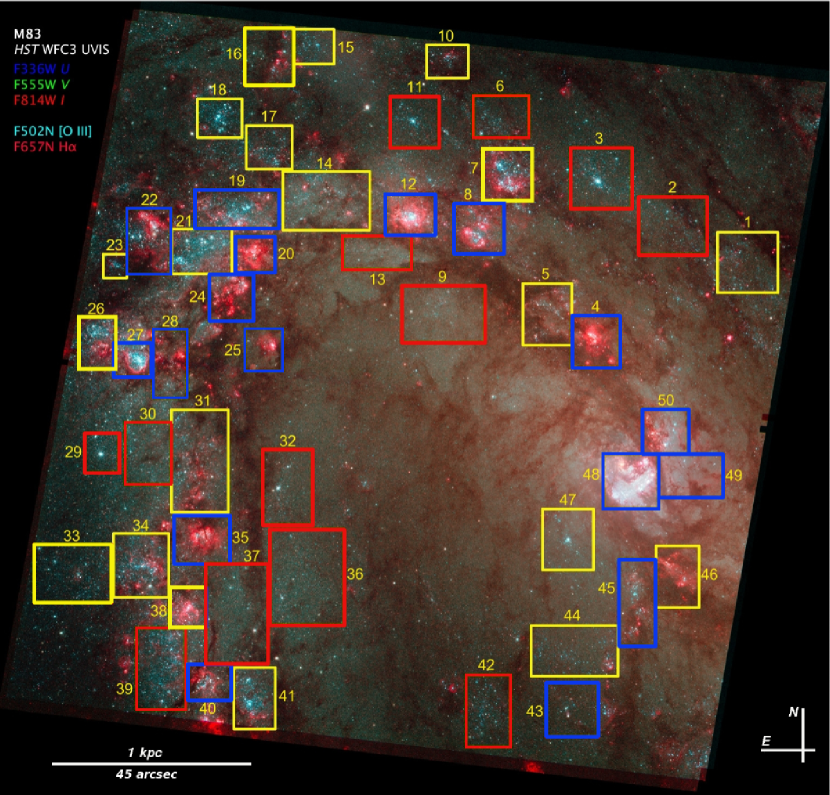
Figure 1.— A color composite of the M83 WFC3 images [Image Credit: Zolt Levay (STScI)]. The F336W image is shown in blue, the F502N ([O III]) image in cyan, the F555W image in green, and the combined F814W and F657N ($H\alpha$) image in red. The 50 selected regions are outlined in boxes of three different colors based on the values of $Age_{CMD}$_auto determined in this paper (see §3.1 for details). The regions with ages in the range 1–10 Myr are outlined in blue, ages of 10–20 Myr in yellow, and ages greater than 20 Myr in red.

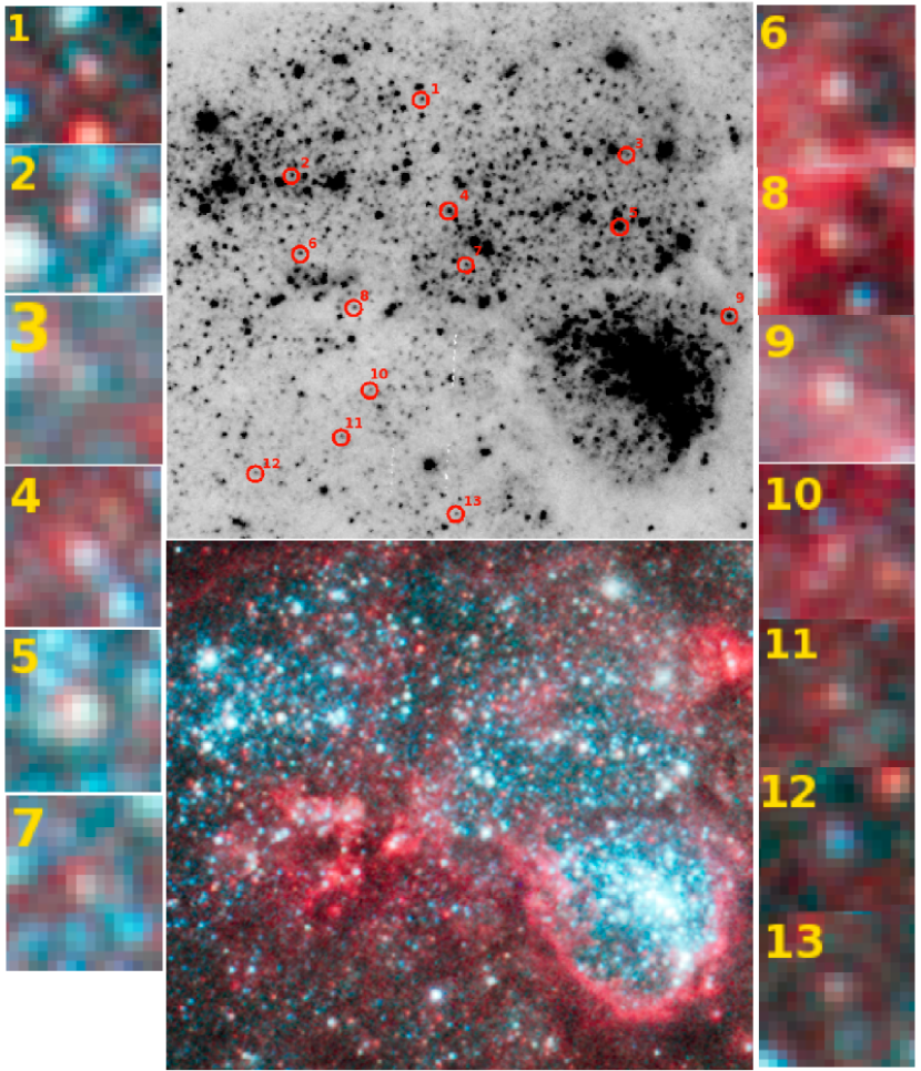
Figure 2.— Image cut-outs (15$\farcs$2$\times$13$\farcs$9, 340 pc$\times$310 pc) of Regions # 26 and # 27 in the F555W ($top$) and the color-composite images ($bottom$). Stars circled in red have $(V-I)>$0.8 mag. The “postage stamp” images on the left are“pseudo” matched candidates, while the images on the right appear to be heavily reddened (see §2.2 for details).

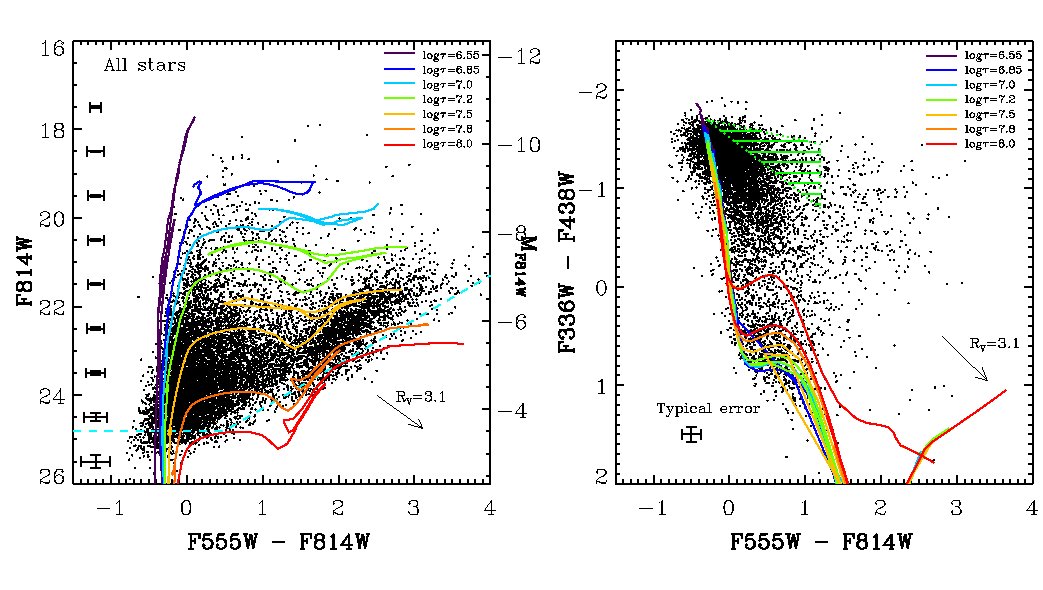
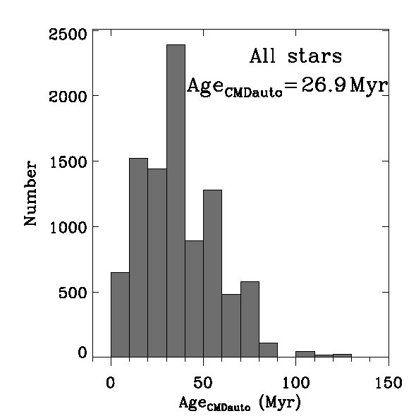
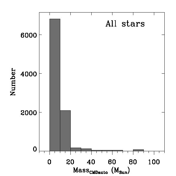
Figure 3.— Top: The color-magnitude diagram (CMD) and color-color diagram of all stars in our M83 image corrected for Galactic foreground extinction but not for internal extinction. Padova isochrones of log$\tau$ (age/yr) = 6.55, 6.85, 7.0, 7.2, 7.5, 7.8, and 8.0 for a metallicity of Z=0.03 (1.5 Z_⊙) are overlaid in both panels. The dashed line in cyan represents the 50% photometric completeness level. The arrow in each panel indicates the direction of the reddening vector with $R_{V}=3.1$. Magnitudes are on the Vega scale. The distance modulus $(m-M)_{0}=28.32$ mag is used to calculate the absolute magnitude $M_{F814W}$. Bottom: Histograms of the distribution of ages and masses, as determined from the CMD (see §3.1 for details). The age quoted in the bottom left panel is the luminosity-weighted mean age.

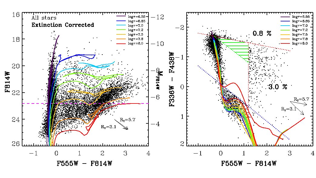
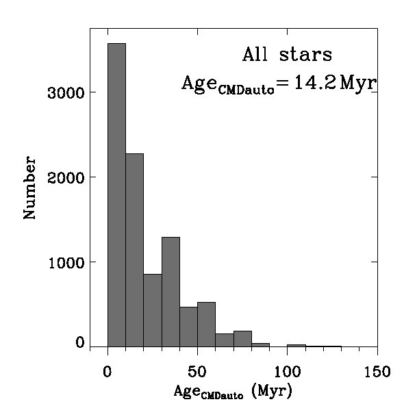
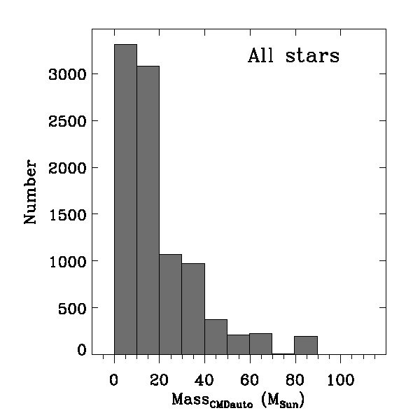
Figure 4.— Top: The CMD and color-color diagram of all stars corrected for the internal extinction determined for each individual star. The blue and two red dotted lines indicate boundaries for the locations of stars in the color-color diagram uncorrected for internal extinction (see §2.4 for discussion). Two arrows in the color-color diagram show reddening vectors: one with the standard reddening vector ($R_{V}=3.1$) and the other with the flatter reddening vector ($R_{V}=5.7$) which appears to be more appropriate for some of the data in the green triangle (see §2.4 for discussion). The dashed line in magenta shows the $M_{I}$$<$$-5.5$ magnitude cutoff used for the $Age_{CMDauto}$ estimate. Bottom: Same as described in Fig. 3.

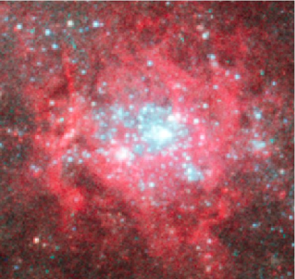
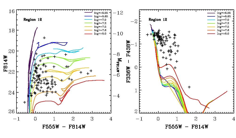
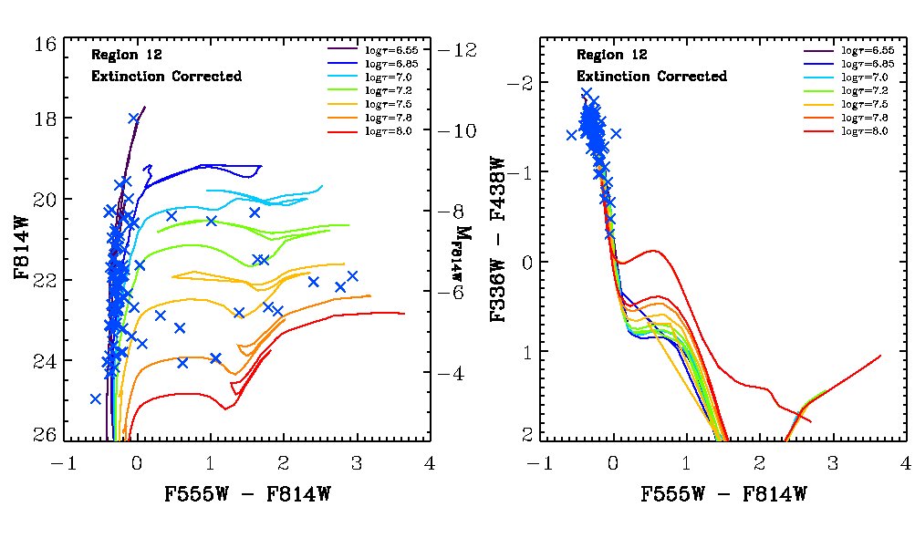
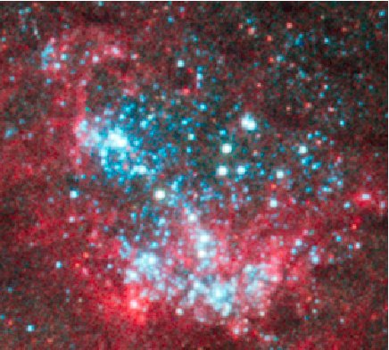
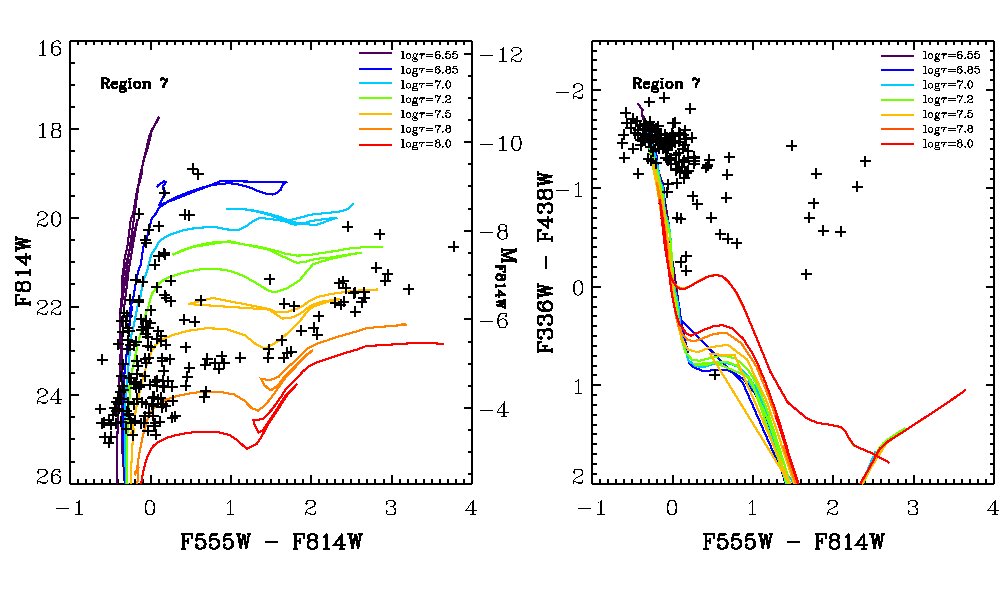
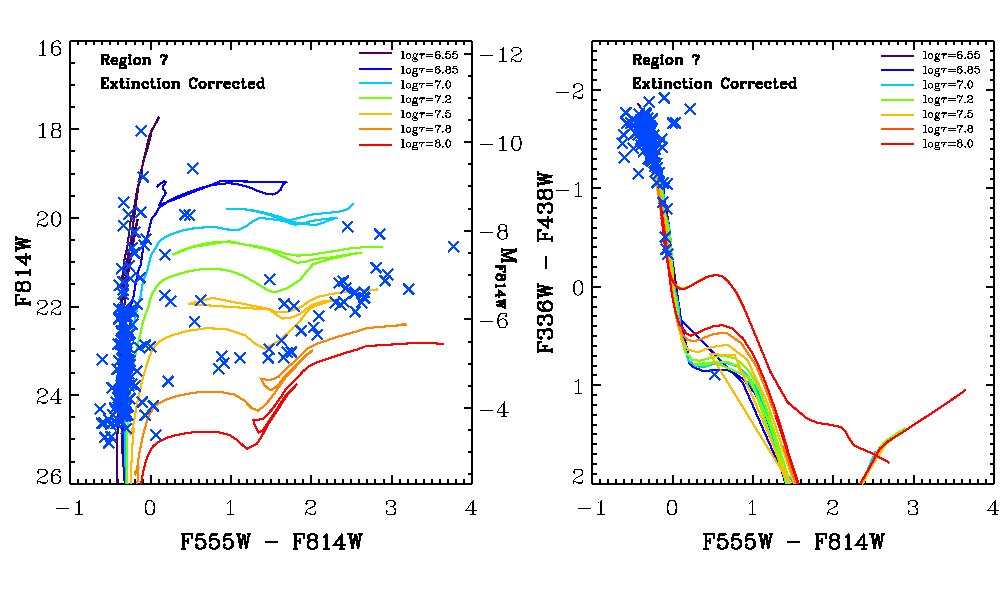
Figure 5.— The CMDs, color-color diagrams and the image cut-outs of Regions # 12 and # 7. Data points before and after the individual extinction correction are plotted as black crosses (upper: uncorrected) and blue Xs (lower: corrected). The Padova isochrones in these diagrams are the same as the ones plotted in Figure 3. See §2.4 for details.

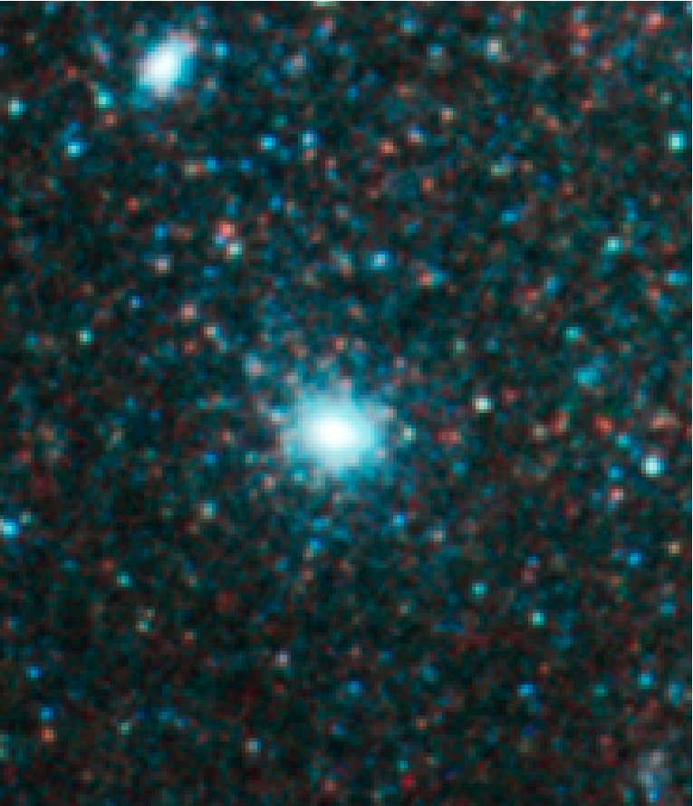
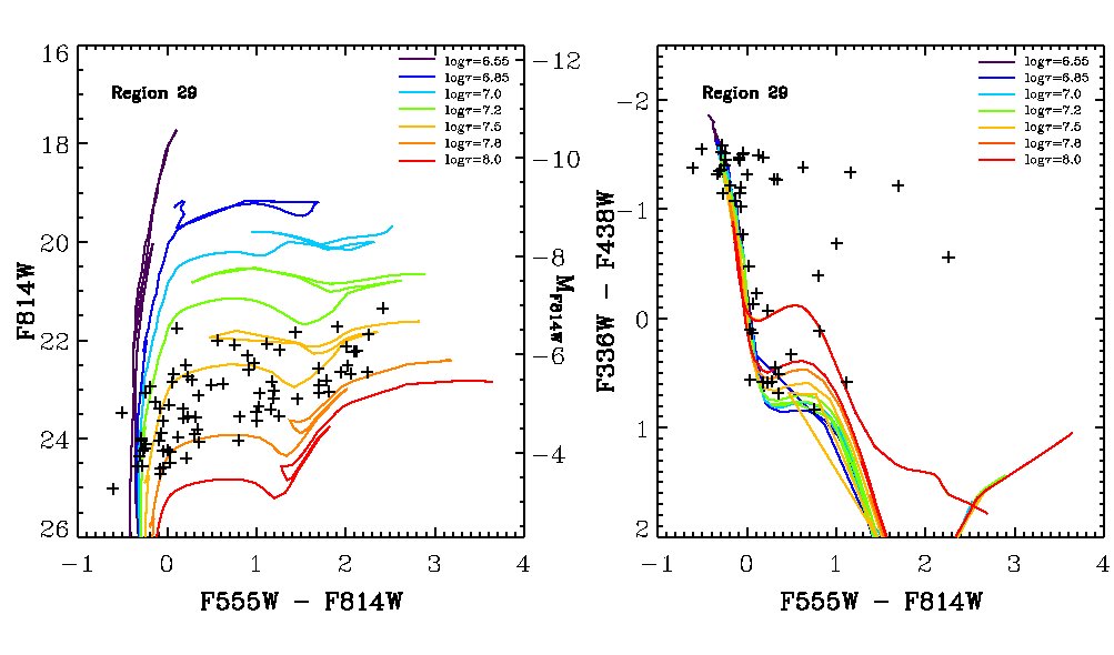
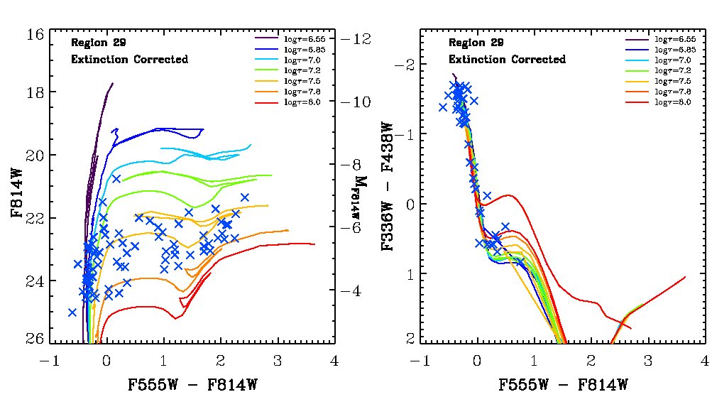
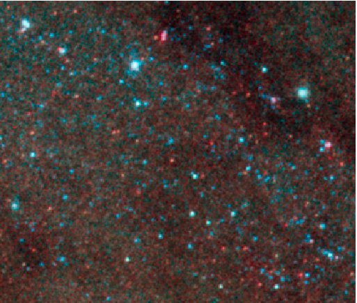
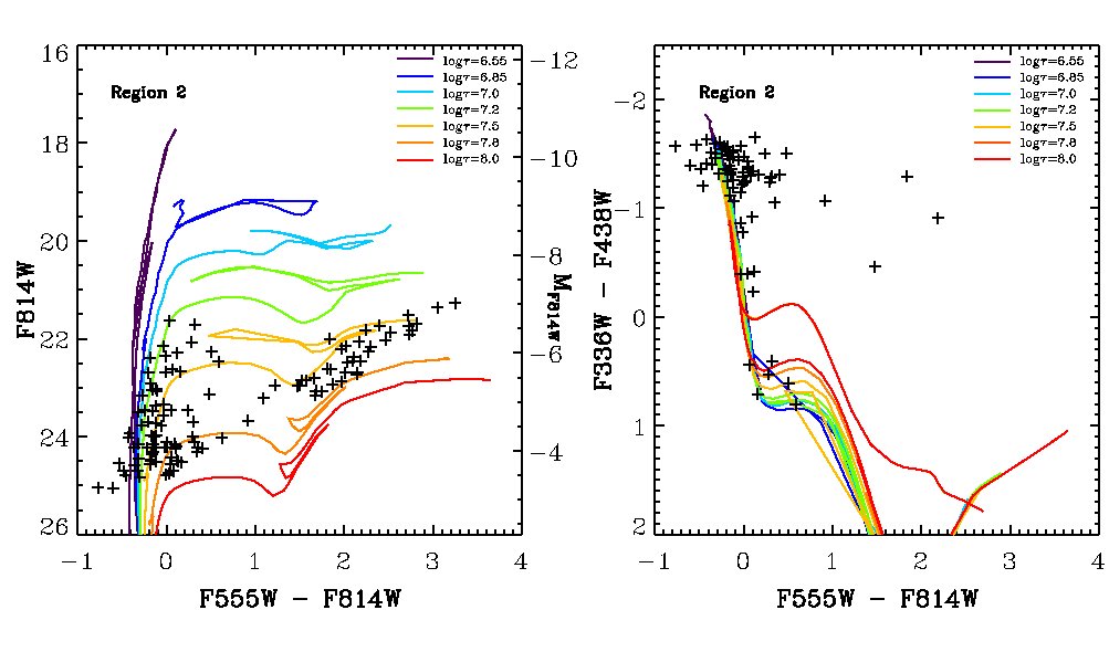
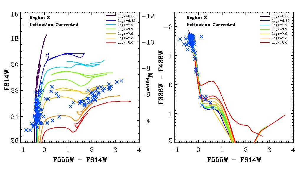
Figure 6.— Same as Figure 5 for Regions # 29 and # 2.

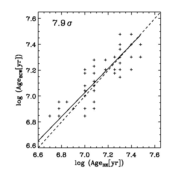
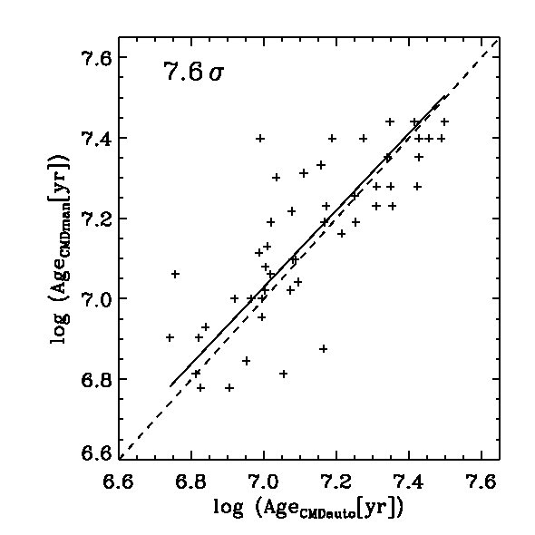
Figure 7.— Correlation plots between the ages of the stellar populations in the 50 regions from CMD isochrone fitting. $(Left)$: Correlation between the manual ages determined by HK and BCW. $(Right)$: Correlation between the average of manual ages and automatic ages (see §3.1 for details). The best linear fits are shown in black with the significance of the correlation in unit of $\sigma$ (i.e., slope/uncertainty) in the top left of each panel. The dashed line is the unity line.

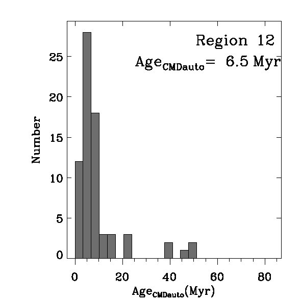
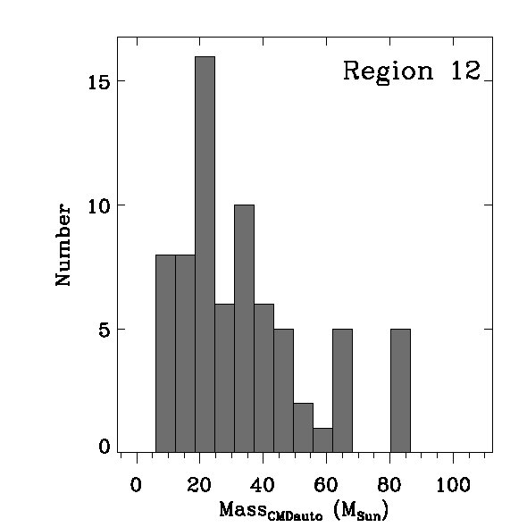
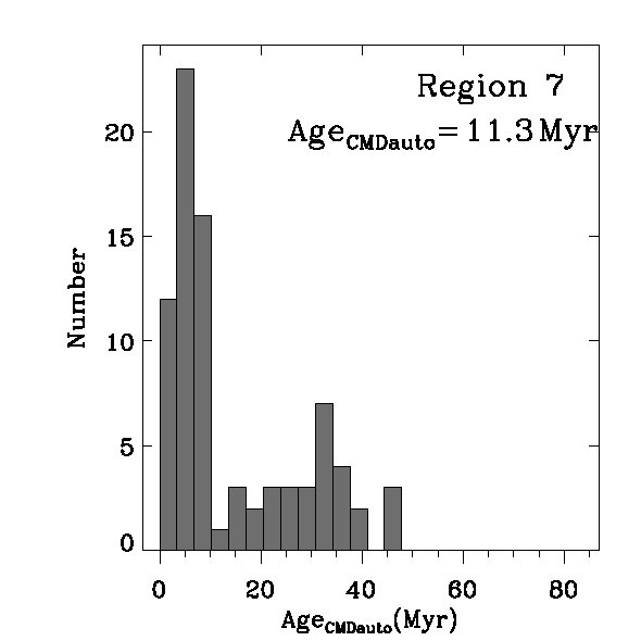
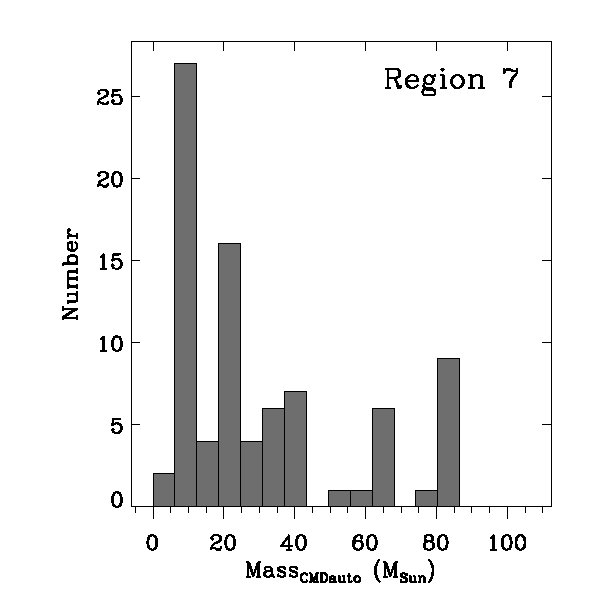
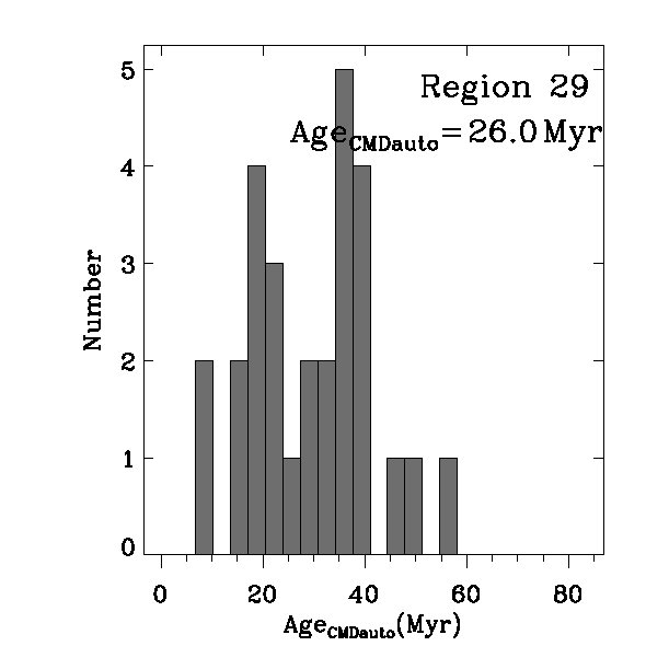
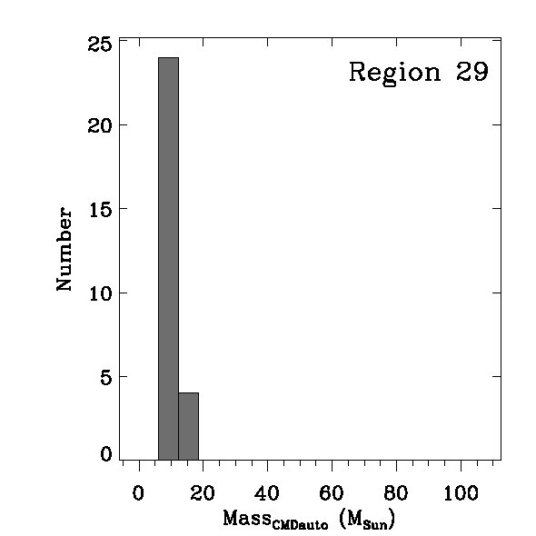
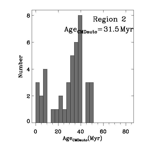
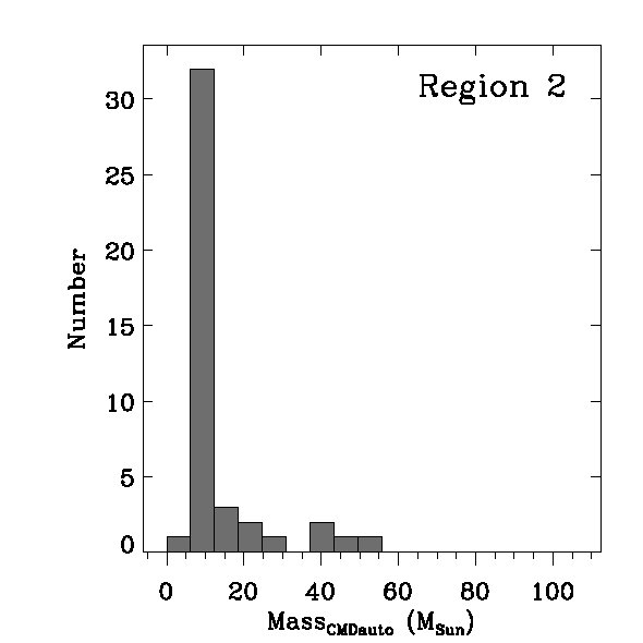
Figure 8.— Histograms of the distribution of ages and masses of the individual stars in Regions # 12, # 7, # 29, and # 2, as determined by the automated isochrone fitting technique (see §3.1). The age indicated at the top right in each age histogram is the luminosity-weighted mean age of all stars with $M_{I}$$<$$-5.5$ in each region.

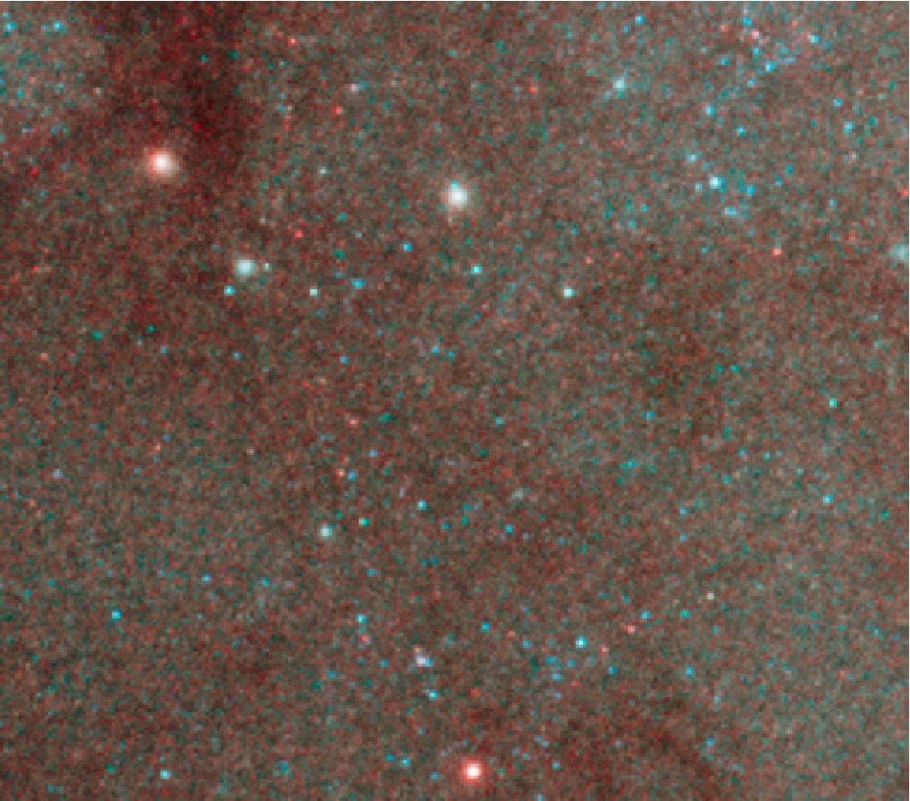
Figure 9.— Image cutout (18$\farcs$3$\times$16$\farcs$9, 410 pc$\times$380 pc) of the area near Region 9 as an example of a “field” region with old red giant stars, and a small population of isolated young blue stars. See §3.1 for for detail.

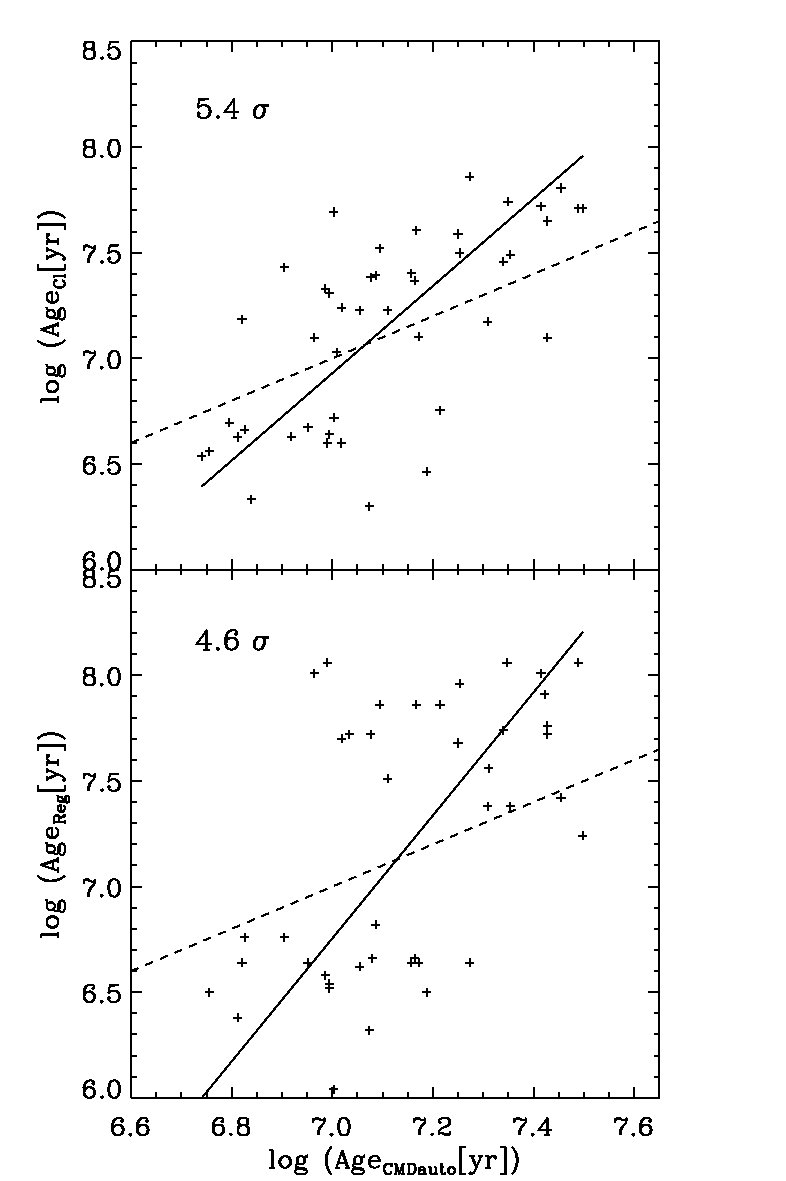
Figure 10.— ($Top$): Correlations between the ages of stars ($Age_{CMD}$_auto) and clusters ($Age_{Cl}$). ($Bottom$): Correlation between the ages of stars determined by $Age_{CMD}$_auto and the integrated light within the region ($Age_{Reg}$). See §3.4 for details. The best linear fits are shown in black solid line with 5.4 $\sigma$ $(top)$ and 4.6 $\sigma$ $(bottom)$ correlations. The dashed line is the unity line.

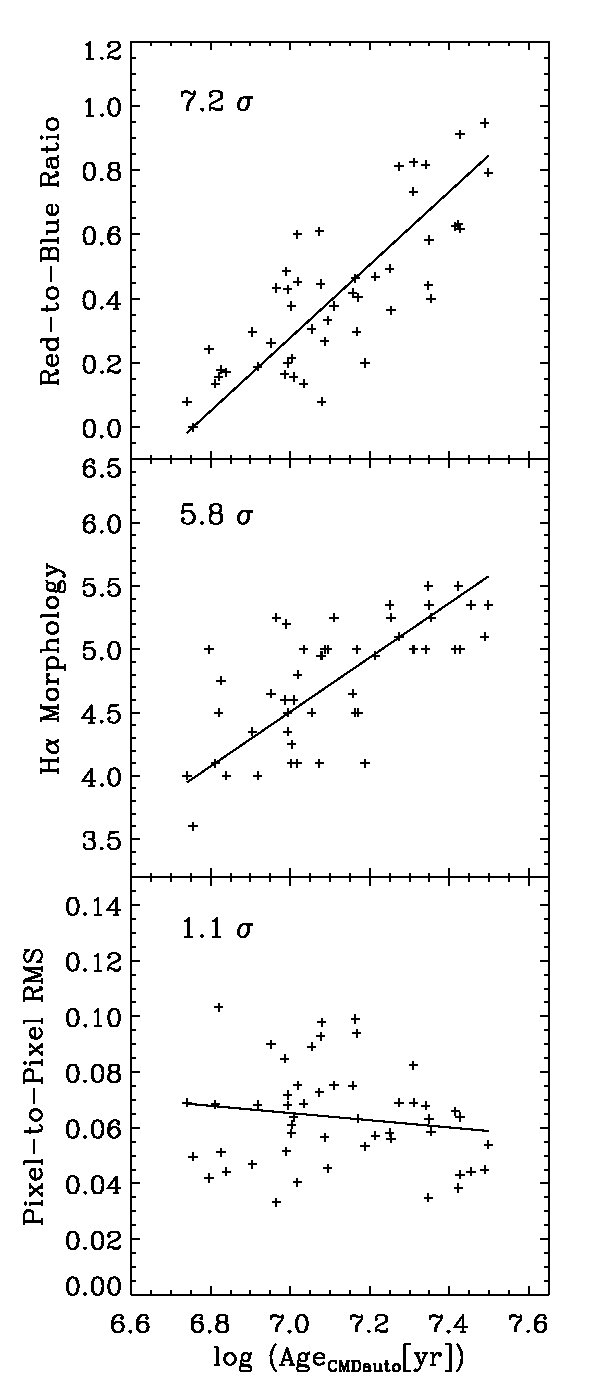
Figure 11.— Correlations between the stellar ages ($Age_{CMD}$_auto) and the number ratio of red-to-blue stars $(top)$, H$\alpha$ morphology $(middle)$, and pixel-to-pixel fluctuations $(bottom)$ for the 50 selected regions. See §4 for details. The best linear fits are indicated in solid black line with 7.2 $\sigma$ $(top)$, 5.8 $\sigma$ $(middle)$, and 1.1 $\sigma$ $(bottom)$ correlations.

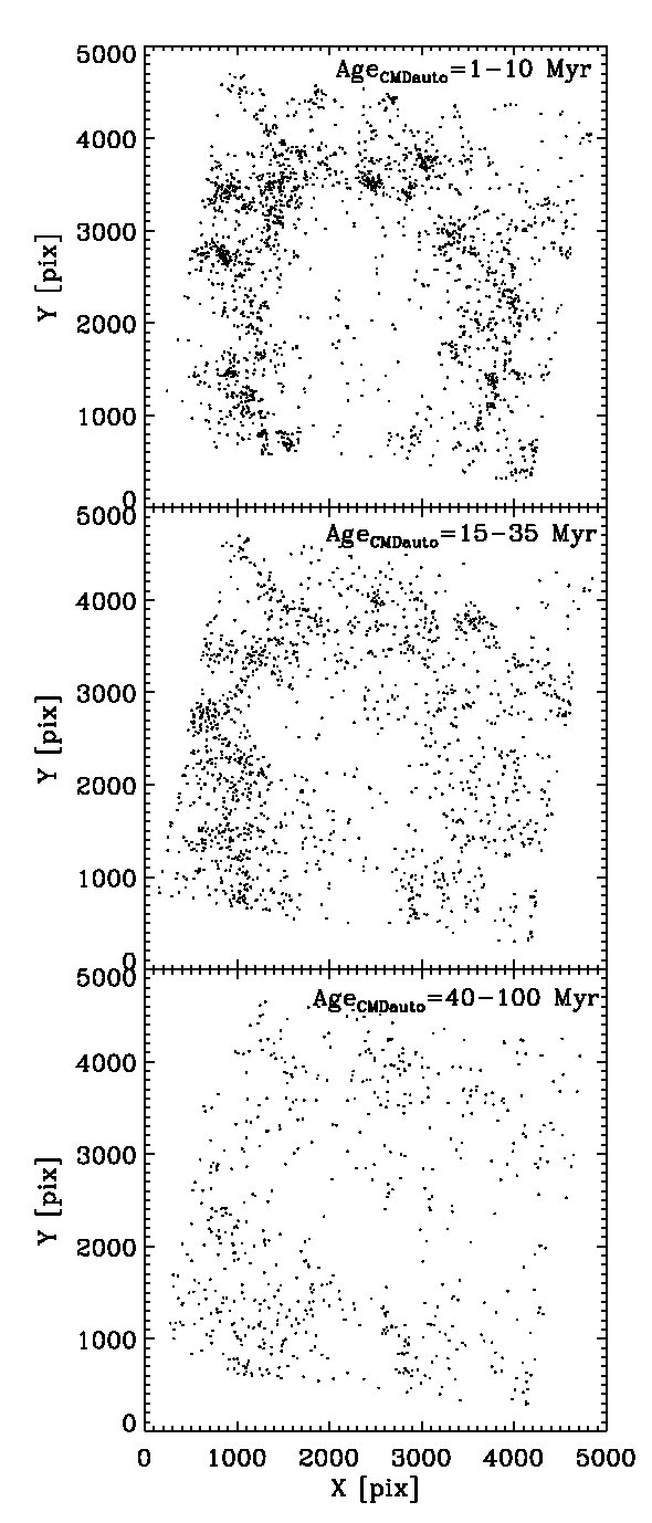
Figure 12.— Spatial distribution of stars with ages of 1–10, 15–35, and 40–100 Myr determined in this study. Each panel has the same orientation and scale as Figure 1. The top panel is the youngest group of stars, clearly showing that the stars in these regions are mostly distributed along the active star-forming region (i.e., associated with the strong H$\alpha$ emission) in the spiral arms. The stars in the middle panel tend to be found slightly downstream of the spiral arms while the older stars are still farther out in the inter-arm regions, as expected. See §5 for details.

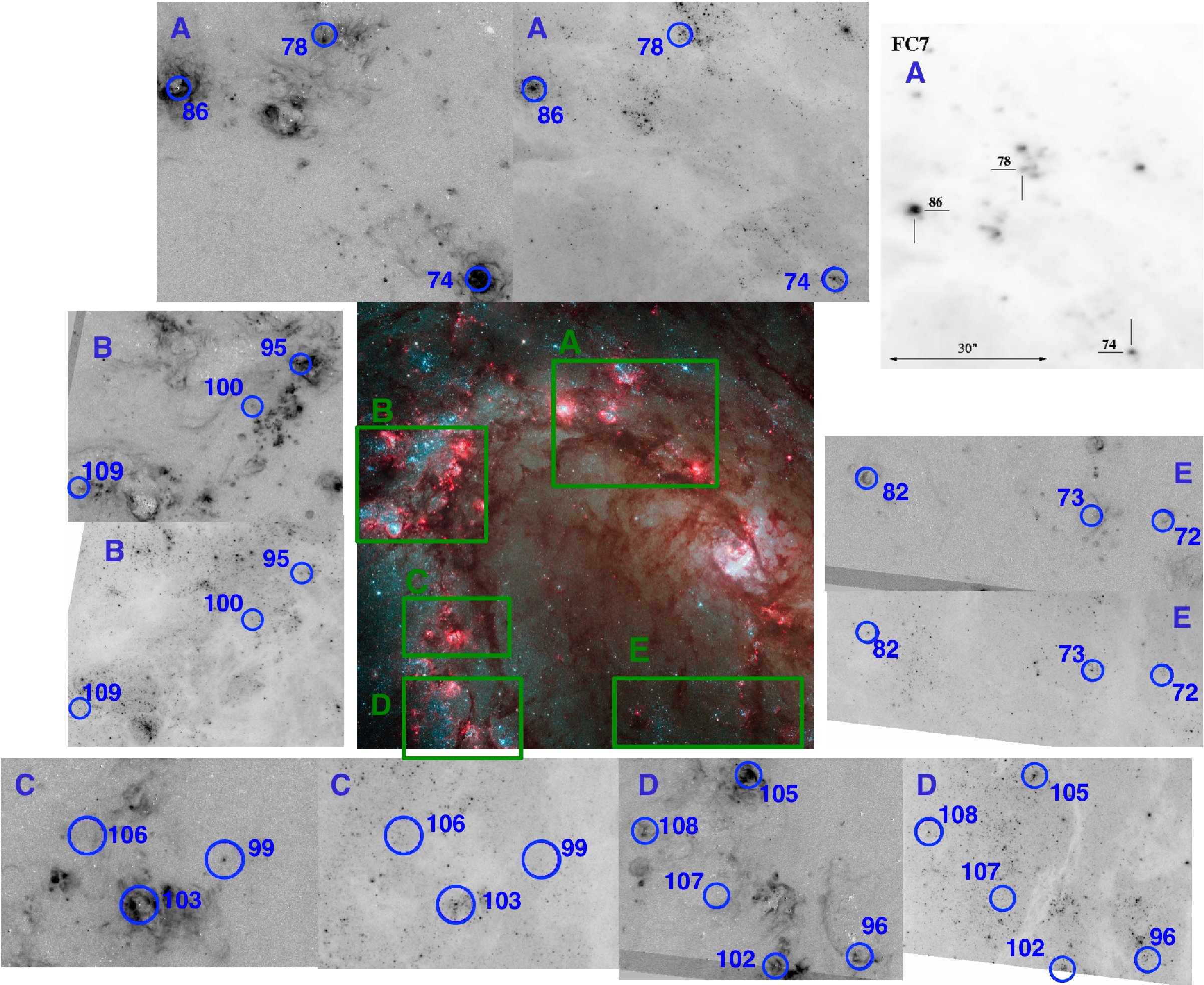
Figure 13.— Distribution of Wolf-Rayet sources in our $HST$ WFC3 M83 images. The color image at the center is the $UBVIH\alpha$ composite and the image cut-outs are the H$\alpha$ ($left$ or $top$) and F814W ($right$ or $bottom$) images for regions A–E. The top right panel is an original finding chart (Hadfield et al., 2005, $\lambda$4684 narrow-band FORS2 image) for the region A. Numbers in blue are the IDs of Wolf-Rayet sources identified by Hadfield et al. (2005).

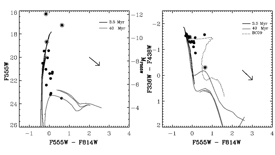
Figure 14.— The CMD and color-color diagram of Wolf-Rayet sources in M83 marked in Figure 13. Three sources (# 78, 86, 105) circled in both diagrams are identified as clusters in our M83 WFC3 images. A twice solar metallicity BC09 cluster model (Bruzual & Charlot 2009, private communication; see also Bruzual & Charlot 2003) is shown in the right panel (dots), and Padova stellar models (Marigo et al., 2008) are shown in both panels. No correction has been made for internal reddening, which appears to be minimal for all but one object. The arrow indicates the Galactic reddening vector.

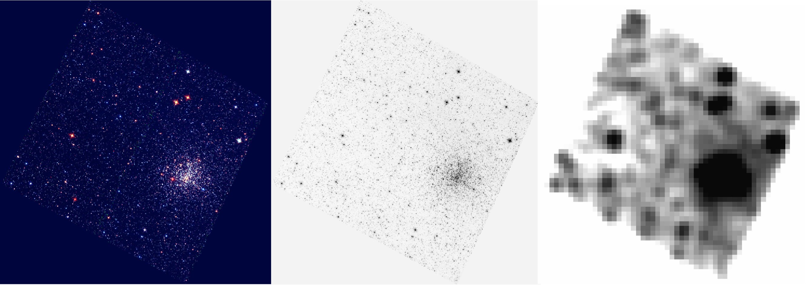
Figure 15.— $HST$/ACS images (290$\arcsec\times$290$\arcsec$, 68 pc$\times$68 pc) of the compact star cluster NGC 2108 in the LMC: a color composite of the F435W, F555W, and F814W ACS images ($left$), the F555W ACS image ($middle$), and the degraded F555W ACS image ($right$) by a factor of 100 (from a distance of $\sim$50 kpc to a distance of $\sim$5 Mpc). See Appendix B for details.

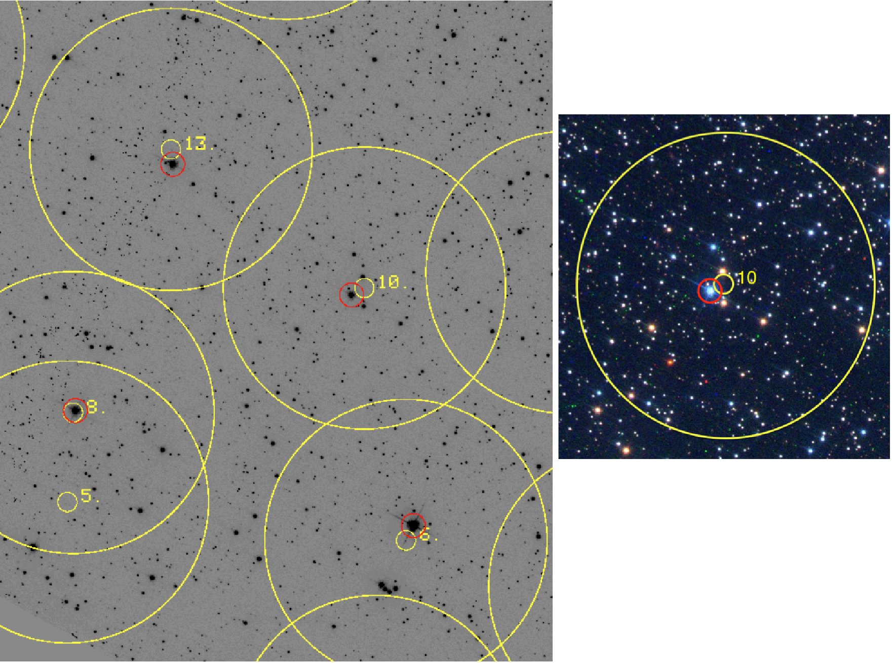
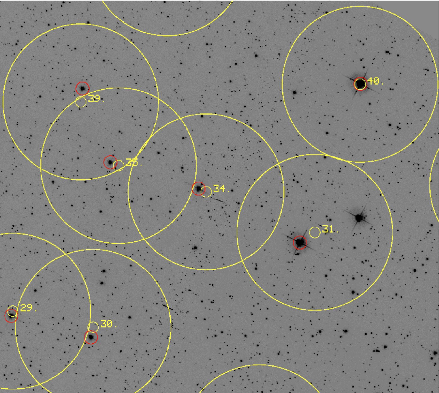
Figure 16.— Image cutouts of $HST$/ACS F555W image of NGC 2108. The large circles in yellow show the 300-pixel aperture (corresponding to a $\sim$3 pixel aperture at the distance of M83) centered at the location determined from the degraded image in Figure 15. The location of the dominant star (used to determine the “truth” value) is shown in red. See Appendix B for details.

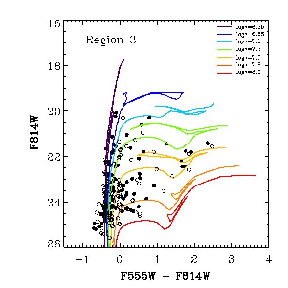
Figure 17.— The original CMD of Region 3 in M83 (solid points) with the effect of simulation representing a factor of 100 degration in spatial resolution (open points). The $Age_{CMD}$_auto of this region changes from 21.9 Myr (determined from the solid points) to 23.8 Myr (from the open points). The difference in the age estimates is within $\sim 1\,\sigma$ error listed in Table 1. See Appendix B for details.

Table 1. Properties of the 50 regions
Region	R.A.(J200)	Dec.(J2000)	Region Size	$Age_{CMD}$man	$Age_{CMD}$auto	$\Delta$$Age^{a}$	$Age_{Reg}^{b}$	$Age_{Cl}^{c}$	Pixel-to-Pixel	Red-to-blue	$H\alpha$	$A_{V}^{d}$	NStar	NCl
	(hh:mm:sec)	(°:’:”)	(pc$\times$pc)	(Myr)	(Myr)	(Myr)	(Myr)	(Myr)	RMS	Ratio	Morphology	(Mag)
1	13:36:59.78	-29:52:30.19	310$\times$310	18.0	17.8	1.8	47.9	38.8	0.0582	0.493	5.35	0.288	206	3
2	13:37:01.11	-29:52:21.60	350$\times$290	27.5	31.5	2.2	17.4	51.3	0.0539	0.792	5.35	0.214	231	2
3	13:37:02.40	-29:52:10.72	310$\times$310	22.5	21.9	1.7	28.7	28.7	0.0679	0.817	5.00	0.161	311	5
4	13:37:02.48	-29:52:48.35	250$\times$260	8.5	6.9	0.5	—	2.2	0.0442	0.171	4.00	0.858	67	4
5	13:37:03.35	-29:52:42.20	240$\times$290	12.5	12.2	1.0	6.6	24.8	0.0566	0.267	5.00	0.677	174	2
6	13:37:04.18	-29:51:56.32	280$\times$210	17.0	22.6	1.1	24.0	30.9	0.0585	0.400	5.25	0.289	132	1
7	13:37:04.07	-29:52:09.72	250$\times$250	6.5	11.3	1.2	4.2	16.9	0.0891	0.306	4.50	0.305	261	9
8	13:37:04.58	-29:52:22.24	250$\times$260	9.0	9.9	0.5	3.5	20.3	0.0718	0.200	4.35	0.369	198	7
9	13:37:05.22	-29:52:41.88	420$\times$280	27.5	22.3	2.9	114.8	—	0.0349	0.442	5.50	0.542	121	0
10	13:37:05.15	-29:51:43.48	210$\times$170	13.5	10.2	2.6	—	10.7	0.0638	0.156	4.60	0.726	74	3
11	13:37:05.72	-29:51:57.44	240$\times$250	25.0	26.7	1.0	52.5	12.6	0.0639	0.911	5.00	0.186	174	2
12	13:37:05.80	-29:52:18.88	250$\times$200	6.5	6.5	0.3	2.4	4.2	0.0684	0.136	4.10	0.758	133	4
13	13:37:06.42	-29:52:27.48	340$\times$180	19.0	26.5	1.8	81.2	—	0.0383	0.632	5.50	0.378	79	0
14	13:37:07.31	-29:52:15.96	440$\times$310	15.5	17.9	0.9	91.2	31.6	0.0562	0.364	5.25	0.475	323	5
15	13:37:07.53	-29:51:40.04	200$\times$180	20.0	10.8	0.5	52.5	—	0.0686	0.135	5.00	0.322	93	0
16	13:37:08.32	-29:51:42.44	240$\times$300	25.0	15.4	0.6	3.2	2.9	0.0534	0.200	4.10	0.408	108	2
17	13:37:08.31	-29:52:03.56	230$\times$230	20.5	12.9	2.0	32.4	16.9	0.0752	0.377	5.25	0.439	180	4
18	13:37:09.21	-29:51:56.48	230$\times$190	16.5	11.9	0.3	52.5	24.2	0.0928	0.446	4.95	0.204	176	6
19	13:37:08.91	-29:52:17.48	430$\times$180	7.0	8.9	0.5	4.4	4.7	0.0900	0.262	4.65	0.392	288	5
20	13:37:08.62	-29:52:27.07	180$\times$180	10.0	8.3	0.4	0.8	4.3	0.0682	0.188	4.00	0.862	97	2
21	13:37:09.55	-29:52:26.87	320$\times$230	15.5	14.7	0.5	72.4	40.4	0.0939	0.297	5.00	0.303	326	7
22	13:37:10.49	-29:52:24.87	220$\times$320	13.0	9.7	0.6	3.8	21.4	0.0848	0.165	4.60	0.801	248	10
23	13:37:11.07	-29:52:30.76	110$\times$110	12.5	12.0	0.8	4.6	—	0.0979	0.080	4.95	0.510	49	0
24	13:37:09.01	-29:52:37.80	190$\times$250	8.0	5.5	0.5	—	3.4	0.0690	0.079	4.00	0.826	108	3
25	13:37:08.42	-29:52:50.52	180$\times$190	11.5	5.7	1.0	3.2	3.6	0.0497	0.000	3.60	0.627	35	1
26	13:37:11.38	-29:52:48.67	180$\times$260	7.5	14.6	1.1	4.6	23.3	0.0991	0.463	4.50	0.342	224	7
27	13:37:10.73	-29:52:52.56	190$\times$160	8.0	6.6	0.4	4.4	15.3	0.1032	0.157	4.50	0.577	117	6
28	13:37:10.09	-29:52:53.76	160$\times$330	12.0	10.1	0.6	—	5.2	0.0612	0.214	4.25	1.017	126	1
29	13:37:11.31	-29:53:14.47	180$\times$200	27.5	26.0	1.1	102.3	52.5	0.0659	0.625	5.00	0.243	153	1
30	13:37:10.48	-29:53:14.32	240$\times$310	19.0	22.3	0.8	—	55.1	0.0632	0.583	5.35	0.317	253	2
31	13:37:09.57	-29:53:16.20	270$\times$510	17.0	14.8	1.2	4.4	12.7	0.0632	0.404	4.50	0.487	401	4
32	13:37:08.02	-29:53:22.28	240$\times$380	22.5	26.7	3.3	57.5	44.7	0.0432	0.618	5.00	0.306	148	3
33	13:37:11.87	-29:53:41.79	370$\times$270	25.0	18.8	0.9	4.4	72.4	0.0690	0.812	5.10	0.217	375	2
34	13:37:10.65	-29:53:40.31	300$\times$330	21.5	14.4	0.3	4.4	25.2	0.0750	0.418	4.65	0.393	425	6
35	13:37:09.54	-29:53:34.48	260$\times$230	10.5	10.1	0.3	1.1	49.3	0.0576	0.377	4.10	0.782	147	2
36	13:37:07.68	-29:53:43.08	390$\times$490	25.0	30.8	4.4	114.8	51.3	0.0450	0.947	5.10	0.286	309	2
37	13:37:08.93	-29:53:51.84	310$\times$510	25.0	28.5	2.2	26.3	64.1	0.0443	1.865	5.35	0.242	287	4
38	13:37:09.80	-29:53:50.39	180$\times$210	10.5	11.8	1.0	2.1	2.0	0.0727	0.610	4.10	0.520	127	1
39	13:37:10.29	-29:54:04.48	260$\times$410	17.0	20.4	1.0	24.0	14.9	0.0825	0.733	5.00	0.174	440	6
40	13:37:09.39	-29:54:07.59	220$\times$180	10.0	9.9	0.6	3.3	4.4	0.0681	0.429	4.50	0.472	124	1
41	13:37:08.60	-29:54:11.04	200$\times$300	15.5	10.4	0.6	50.1	17.4	0.0752	0.453	4.80	0.449	183	1
42	13:37:04.41	-29:54:14.20	230$\times$370	19.0	20.4	1.5	36.3	—	0.0690	0.825	5.00	0.232	196	0
43	13:37:02.92	-29:54:13.92	250$\times$270	25.0	9.8	0.3	114.8	4.0	0.0516	0.485	5.20	0.300	97	1
44	13:37:02.87	-29:54:00.80	440$\times$260	14.5	16.4	1.0	72.4	5.7	0.0571	0.469	4.95	0.245	224	5
45	13:37:01.77	-29:53:49.24	190$\times$440	6.0	6.7	0.5	5.8	4.6	0.0512	0.179	4.75	0.899	130	6
46	13:37:01.04	-29:53:42.56	220$\times$290	11.5	10.4	0.5	—	4.0	0.0404	0.600	4.10	0.846	82	1
47	13:37:02.99	-29:53:34.17	250$\times$310	11.0	12.4	1.2	72.4	33.1	0.0455	0.333	5.00	0.427	120	2
48e	13:37:01.86	-29:53:20.83	270$\times$290	—	6.2	0.5	—	5.0	0.0419	0.242	5.00	0.406	38	83
49	13:37:00.79	-29:53:19.27	330$\times$220	10.0	9.2	0.2	102.3	12.6	0.0333	0.433	5.25	0.507	55	10
50	13:37:01.24	-29:53:09.23	220$\times$220	6.0	8.0	0.5	5.8	27.0	0.0469	0.296	4.35	0.652	72	12
a$\Delta$$Age_{CMD}$auto is the mean value of the uncertainties in our age determination. See §3.1 for details.
b$Age_{Reg}$ is the region age determined by measuring the colors of the entire regions, and fitting SED. See §3.4 for details.
cThe luminosity-weighted mean age of clusters in each region. Age of each cluster is determined by SED fitting. See §3.3 for details.
d Average value of the extinctions ($A_{V}$) measured from the resolved stars in each region.
eRegion # 48 is the nucleus of M83. It is not included in the analysis since the bright background results in a completeness limit that is more than two magnitudes
brighter than other regions.

Table 2. Wolf-Rayet Star Candidates in M83
RA DEC $ID_{Hadfield}$ Reg# $Age_{Reg}(Myr)$ X Y Comments 13:37:00.41 -29:52:54.1 72 — — 3874 606 faint H$\alpha$ 13:37:01.18 -29:52:53.9 73 — — 3618 609 faint H$\alpha$ 13:37:01.42 -29:51:25.8 74 4 — 3512 2821 strong H$\alpha$ 13:37:03.06 -29:50:49.5 78 7 4.2 2982 3698 faint H$\alpha$ 13:37:04.65 -29:52:47.5 82 — — 2710 772 strong H$\alpha$ 13:37:04.65 -29:50:58.4 86 12 2.4 2477 3505 strong H$\alpha$ 13:37:07.35 -29:49:39.2 95 20 0.8 1513 3306 strong H$\alpha$ 13:37:07.54 -29:52:53.6 96 41 50.1 1552 620 strong H$\alpha$ 13:37:07.96 -29:52:07.9 99 — — 1418 1762 faint H$\alpha$ 13:37:08.25 -29:51:13.6 100 24 — 1311 3116 faint H$\alpha$ 13:37:08.40 -29:52:54.9 102 — — 1266 588 strong H$\alpha$ 13:37:08.53 -29:52:12.0 103 35 1.1 1224 1659 strong H$\alpha$ 13:37:08.70 -29:52:28.9 105 38 2.1 1173 1239 strong H$\alpha$ 13:37:08.91 -29:52:05.7 106 31 4.4 1101 1818 faint H$\alpha$ 13:37:09.02 -29:52:45.2 107 39 24.0 1067 825 no H$\alpha$ 13:37:09.80 -29:52:36.2 108 — — 820 1049 strong H$\alpha$ 13:37:10.42 -29:51:28.0 109 26 4.6 610 2756 faint H$\alpha$

References

- Bastian et al. (2011) Bastian, N., et al. 2011, MNRAS, 417, L6
- Bresolin & Kennicutt (2002) Bresolin, F., & Kennicutt, R. C. 2002, ApJ, 572, 838
- Cardelli et al. (1989) Cardelli, J. A., Clayton, G. C., & Mathis, J. S. 1989, AJ, 345, 245
- Chandar et al. (2010) Chandar, R., et al. 2010, ApJ, 719, 966
- Crowther (2007) Crowther, P. A. 2007, ARA&A, 45, 177
- Dalcanton et al. (2009) Dalcanton, J. J., et al. 2009, ApJS, 183, 67
- Dobbs & Pringle (2010) Dobbs, C. L., & Pringle, J. E. 2010, MNRAS, 409, 396
- Dopita et al. (2010) Dopita, M. A., et al. 2010, ApJ, 710, 964
- Fariña et al. (2012) Fariña, C., Bosch, G. L., & Barbá, R. H. 2012, AJ, 143, 43
- Freedman et al. (2001) Freedman, W. L., et al. 2001, ApJ, 553, 47
- Goudfrooij et al. (2011) Goudfrooij, P., Puzia, T. H., Kozhuria-Platais, V., & Chandar, R. 2011, ApJ, 737, 3
- Hadfield et al. (2005) Hadfield, L. J., Crowther, P. A., Schild, H., & Schmutz, W. 2005, A&A, 439, 265
- Harris et al. (2001) Harris, J., Calzetti, D., Gallagher, J. S., Conselice, C. J., & Smith, D. A. 2001, AJ, 122, 3046
- Karachentsev et al. (2007) Karachentsev, I. D., et al. 2007, AJ, 133, 504
- Koekemoer et al. (2002) Koekemoer, A. M., Fruchter, A. S., Hook, R. N., & Hack, W. 2002, in The 2002 Calibration Workshop: Hubble after the Installation of the ACS and the NICMOS Cooling System, ed. S. Arribas, A. Koekemoer, & B. Whitmore (Baltimore, MD: STScI), 337
- Lada & Lada (2003) Lada, C. J., & Lada, E. A. 2003, ARA&A, 41, 57
- Larsen (2004) Larsen, S. S. 2004, A&A, 416, 537
- Larsen et al. (2011) Larsen, S. S., et al. 2011, A&A, 532, A147
- Marigo et al. (2008) Marigo, P., Girardi, L., Bressan, A., Groenewegen, M. A. T., Silva, L., & Granato, G. L. 2008, A&A, 482, 883
- Mihalas & Binney (1981) Mihalas, D., & Binney, J. 1981, Galactic Astronomy (San Francisco: Freeman), 187
- Pellerin et al. (2007) Pellerin, A., Meyer, M., Harris, J., & Calzetti, D. 2007, ApJ, 658, L87
- Saha et al. (2006) Saha, A., Thim, F., Tammann, G. A., Reindl, B., & Sandage, A. 2006, ApJS, 165, 108
- Saha et al. (2010) Saha, A., et al. 2010, AJ, 140, 1719
- Schechter et al. (1993) Schechter, P. L., Mateo, M., & Saha, A. 1993, PASP, 105, 1342
- Schlegel et al. (1998) Schlegel, D. J., Finkbeiner, D. P., & Davis, M. 1998, ApJ, 500, 525
- Sirianni et al. (2005) Sirianni, M., et al. 2005, PASP, 117, 1049
- Whitmore et al. (1999) Whitmore, B. C., Zhang, W., Leitherer, C., Fall, S. M., Schweizer, F., & Miller, B. W. 1999, AJ, 118, 1551
- Whitmore et al. (2011) Whitmore, B. C., et al. 2011, ApJ, 729, 14
- Whitmore (2011) Whitmore, B. C. & the WFC3 SOC Team 2011, in ASP Conf. Ser. 440, UP2010: Have Observations Revealed a Variable Upper End of the Initial Mass Function?, ed. M. Treyer, T. K. Wyder, J. D. Neill, M. Seibert, and J. C. Lee (San Francisco, CA: ASP), 161
- Windhorst et al. (2011) Windhorst, R. A., et al. 2011, ApJS, 193, 27