2D Radiative MHD Simulations of the Importance of Partial Ionization in the Chromosphere

Abstract

The bulk of the solar chromosphere is weakly ionized and interactions between ionized particles and neutral particles likely have significant consequences for the thermodynamics of the chromospheric plasma. We investigate the importance of introducing neutral particles into the MHD equations using numerical 2.5D radiative MHD simulations obtained with the Bifrost code. The models span the solar atmosphere from the upper layers of the convection zone to the low corona, and solve the full MHD equations with non-grey and non-LTE radiative transfer, and thermal conduction along the magnetic field. The effects of partial ionization are implemented using the generalized Ohm’s law, i.e., we consider the effects of the Hall term and ambipolar diffusion in the induction equation. The approximations required in going from three fluids to the generalized Ohm’s law are tested in our simulations. The Ohmic diffusion, the Hall term, and ambipolar diffusion show strong variations in the chromosphere. These strong variations of the various magnetic diffusivities are absent or significantly underestimated when, as has been common for these types of studies, using the semi-empirical VAL-C model as a basis for estimates. In addition, we find that differences in estimating the magnitude of ambipolar diffusion arise depending on which method is used to calculate the ion-neutral collision frequency. These differences cause uncertainties in the different magnetic diffusivity terms. In the chromosphere, we find that the ambipolar diffusion is of the same order of magnitude or even larger than the numerical diffusion used to stabilize our code. As a consequence, ambipolar diffusion produces a strong impact on the modeled atmosphere. Perhaps more importantly, it suggests that at least in the chromospheric domain, self-consistent simulations of the solar atmosphere driven by magneto-convection can accurately describe the impact of the dominant form of resistivity, i.e., ambipolar diffusion. This suggests that such simulations may be more realistic in their approach to the lower solar atmosphere (which directly drives the coronal volume) than previously assumed.

1 Introduction

Most of the models and simulations of the solar atmosphere solve the magnetohydrodynamics (MHD) equations, implicitly assuming that the plasma is magnetized, i.e., fully ionized or with the ion-neutral collision frequency lower than the ion gyrofrequency (Schaffenberger et al., 2005; Vögler et al., 2005; Stein & Nordlund, 2006; Gudiksen et al., 2011, among others). However, since the photosphere and parts of the chromosphere are unmagnetized, i.e., the ions are not necessarily tied to the field lines, we expect that neutral particles can have a significant impact on the dynamics of this region (Vernazza et al., 1981; Fontenla et al., 1990, 1993). Therefore, it is likely that, under some conditions, the photosphere and chromosphere should be treated as a three component fluid, where the dynamics of the neutrals, ions, and electrons are treated separately. Under the assumption of a weakly ionized plasma, one can return to a one-component fluid. However, new terms known as the Hall term and ambipolar diffusion appear in the induction equation (Parker, 1963, 2007; Pandey & Wardle, 2008). The latter term is a consequence of the ion-neutral dissipation which can be derived from the Cowling resistivity (Khodachenko et al., 2004, 2006; Leake & Arber, 2006). This form of the induction equation is known as the generalized Ohm’s law (Cowling, 1957).

A large number of papers in recent years have investigated the effects of the ion-neutral interactions on single fluid MHD. Leake & Arber (2006) simulated 2.5D simulations of flux emergence and observed that the ambipolar diffusion leads to an increase of the rates of magnetic field emergence and a resultant magnetic field that is much more diffuse than the case with only Ohmic diffusivity. In addition, the magnetic field that emerges into the corona is found to be more force-free, since currents are aligned to the field. This is because ambipolar diffusion acts on the currents perpendicular to the magnetic field. Arber et al. (2007) extended this simulation to 3D where the previous results were confirmed, and in addition found that, as a result of including neutrals, flux emergence lifts less chromospheric material to great heights. This effect suppresses the Rayleigh-Taylor instability between the emerging flux and the corona.

The interaction between ions and neutrals can also dissipate Alfvén waves as result of the small but finite coupling time between ions and neutrals. This type of damping can heat and accelerate the plasma in the upper chromosphere and in spicules (De Pontieu & Haerendel, 1998; De Pontieu, 1999; James & Erdélyi, 2002; James et al., 2003; Erdélyi & James, 2004) and incur wave energy leakage at the footpoints of coronal loops (De Pontieu et al., 2001) and in the network (Goodman, 2000). Khodachenko et al. (2004), using the temperature and density structure from the 1D VAL-C model, concluded that the collisional friction damping of MHD waves is often more important than the viscous damping for waves propagating in the partially ionized plasmas of the solar photosphere, chromosphere and prominences. Estimates of the efficiency of the damping of waves were made by Leake et al. (2005) as well as by the previous authors.

Pandey & Wardle (2008) determine that waves can be affected by the Hall term at both low and high fractional ionization, because the Hall regime wave damping is inversely proportional to the fractional ionization. Thus Hall term may also be important at high fractional ionization in contrast to ambipolar diffusion which is important only at low fractional ionization.

Khomenko & Collados (2012) performed various simplified scenarios where they studied the impact of the ambipolar diffusion in the chromosphere. They conclude that current dissipation enhanced by the action of ambipolar diffusion is an important process that is able to provide a significant energy input into the chromosphere. Heating from ambipolar diffusion leads to thermodynamic evolution in the chromosphere on timescales of about 10–100 seconds.

All the models above, even the 2D and 3D models, are based on a 1D semi-empirical atmosphere (e.g., VAL-C), and/or a simplified approach to the energy balance in the chromosphere (adiabatic or Newtonian cooling). In addition, none of the partial ionization effects have been considered in full magneto-convection simulations. Cheung & Cameron (2012) have made progress in this direction and performed full magneto-convection simulations of an umbra taking into account partial-ionization effects. However, their simulations only extend up to the upper photosphere.

In this paper, we use the Bifrost code (Gudiksen et al., 2011) to create a self-consistent and fully dynamic model atmosphere of the sun, from the convection zone to the corona, to consider the importance of the Hall term and ambipolar diffusion relative to the Ohmic and artificial diffusion. Unlike other models, Bifrost includes an advanced treatment of radiative losses in the chromosphere based on recipes derived from dynamic non-LTE radiative 1D hydrodynamic simulations. Such a treatment is crucial for a consideration of the effects of partial ionization, as shown in what follows. The code and the implementation of the generalized Ohm’s law are described in Section 2. The tests performed for the code validation are discussed in Section 2.2. We describe the different forms of diffusion in 2D MHD simulations in Section 3.1. Finally, the various simplifications made in order to obtain the generalized Ohm’s law following Pandey & Wardle (2008) have been investigated and tested for the 2D MHD simulations in Section 3.2. The paper finishes by addressing the conclusions and discussion.

2 Equations and numerical method

The magnetic upper-photosphere and chromosphere is weakly ionized and the interaction between ionized particles and neutral particles potentially has important consequences for the thermodynamics (Fontenla et al., 1993) of this region. We investigate these consequences in the solar atmosphere. In order to model the solar atmosphere we solve the MHD equations in $2.5$D. The model spans from the upper layers of the convection zone to the low corona. We have implemented the effects of partial ionization into the induction equation through the Hall and ambipolar diffusion terms as described below.

The Bifrost (Gudiksen et al., 2011) code is a staggered mesh, explicit code that solves the MHD partial differential equations, including non-LTE and non-grey radiative transfer with scattering, and conduction along the magnetic field lines. A lookup table, based on LTE, is used to compute the temperature, pressure, opacities and other radiation quantities, and ionization state, given the pressure and the internal energy of the plasma. Spatial derivatives and the interpolation of variables are done using high order polynomials. The equations are stepped forward in time using the explicit third order predictor-corrector procedure described by Hyman et al. (1979). In order to suppress numerical noise, high-order artificial diffusion is added both in the forms of a viscosity and in the form of a magnetic diffusivity (see Gudiksen et al., 2011, for details).

The Bifrost code includes an advanced treatment of the effects of radiation on the local energy balance, which is crucial if one wants to accurately determine the ionization degree. The radiative flux divergence from the photosphere and lower chromosphere is obtained by angle and wavelength integration of the transport equation assuming isotropic opacities and emissivities. The transport equation assumes that opacities are in LTE using four group mean opacities to cover the entire spectrum (Nordlund, 1982). This is done by formulating the transfer equation for each of the four bins, calculating a mean source function in each bin. These source functions contain an approximate coherent scattering term and an exact contribution from thermal emissivity. The resulting 3D scattering problems are solved by iteration, based on one-ray approximation in the angle integral for the mean intensity, a method developed by Skartlien (2000).

In the mid and upper chromosphere, the Bifrost code includes non-LTE radiative losses from tabulated hydrogen continua, hydrogen lines, and lines from singly ionized calcium as functions of temperature and column mass (Carlsson & Leenaarts, 2012). These radiative losses depend on the computed non-LTE escape probability as a function of column mass and are based on a 1D dynamical chromospheric model in which the radiative losses are computed in detail (Carlsson & Stein, 1992, 1994, 1997, 2002).

The energy dissipated by Joule heating is given by $Q_{Joule}={\bf E\cdot J}$ where the electric field ${\bf E}$ is calculated from the current ${\bf J}$, taking into account high-order artificial resistivity. The resistivity is computed using a hyper-diffusion operator (Gudiksen et al., 2011). This entails that the Joule heating due artificial diffusion is set proportional to the current squared times a factor that becomes large (of order 10) when magnetic field gradients are large, and is unity otherwise.

2.1 Generalized Ohm’s Law theory

2.1.1 Multi-fluid

Most codes treat the solar atmosphere as a single fluid where collisional frequencies are considered sufficient to ensure that all species are well coupled and that the momentum and energy equations can be added without the introduction of frictional terms or similar. However, as chromospheric temperatures are likely to drop to a few $10^{3}$ K or even lower (Leenaarts et al., 2011), there is a high probability that plasma is only partially ionized and that “slippage” effects could become important. In this case the MHD equations should be treated by considering the plasma to consist of three fluids: ions, electrons and neutral particles. The mass density for each type of particle is governed by the continuity equation applied to each species separately:

$$\frac{\partial\rho_{j}}{\partial t}+\nabla\cdot\rho_{j}{\bf u_{j}}=0$$ (1)

where $\rho_{j}=m_{j}n_{j}$, ${\bf u_{j}}$, $n_{j}$ and $m_{j}$ are the mass density, velocity, number density and particle mass of the ion, electron, and neutral species, i.e., $j=\mathrm{i,e,n}$ respectively. The mass transfer term as result of ionization and recombination has been neglected. This approximation is valid for a one-fluid approach if the system is in ionization balance, and there is no decoupling of ions and neutrals.

The momentum equation, written in SI units, for each species, is as follows:

$$\rho_{i}\left(\frac{\partial}{\partial t}+{\bf u_{i}}\cdot\nabla\right){\bf u_{i}}=-\nabla P_{i}+n_{i}Zq_{e}\left({\bf E}+{\bf u_{i}}\times{\bf B}\right)-\rho_{i}\sum_{j=e,n}\nu_{ij}({\bf u_{i}-u_{j}})$$ (2)

$$\rho_{e}\left(\frac{\partial}{\partial t}+{\bf u_{e}}\cdot\nabla\right){\bf u_{e}}=-\nabla P_{e}-n_{i}q_{e}\left({\bf E}+{\bf u_{e}}\times{\bf B}\right)-\rho_{e}\sum_{j=i,n}\nu_{ej}({\bf u_{e}-u_{j}})$$ (3)

$$\rho_{n}\left(\frac{\partial}{\partial t}+{\bf u_{n}}\cdot\nabla\right){\bf u_{n}}=-\nabla P_{n}-\rho_{n}\sum_{j=e,i}\nu_{nj}({\bf u_{n}-u_{j}})$$ (4)

where $q_{e}$ and $Z$ are respectively the electron charge and ion charge. ${\bf E}$ and ${\bf B}$ are the electric and magnetic field and $P_{j}=n_{i}kT_{i}$ is the partial pressure of the $j$th species, $k$ is Boltzmann’s constant, and $\nu_{ij}$ is the collision frequency for species $i$ with species $j$. We assume that collisions are sufficiently numerous that the ion and electron temperature can be considered the same ($T_{i}=T_{e}$). All three equations are linked through the last term, i.e., the exchange of momentum between the particles, where we have ignored the thermal force. In a similar manner as for the continuity equation, the momentum transfer term as result of ionization and recombination has been neglected.

The number of equations thus increases considerably compared with single fluid MHD, but by considering some simplifications, as described by Cowling (1957); Parker (2007); Pandey & Wardle (2008), one can easily generalize the MHD equations for each species to a single fluid (see below too). Therefore, the mass density is governed by the continuity equation for the bulk fluid as follows:

$$\frac{\partial\rho}{\partial t}+\nabla\cdot\rho{\bf u}=0$$ (5)

where the density for the bulk fluid is the sum of the different particle densities ($\rho=\rho_{i}+\rho_{e}+\rho_{n}$), and considering $\rho_{i}/\rho>>\rho_{e}/\rho$, then $\rho\approx\rho_{i}+\rho_{n}$. In a similar manner, the velocity of the bulk fluid is ${\bf u}\approx(\rho_{i}{\bf u_{i}}+\rho_{n}{\bf u_{n}})/\rho$, where the electron inertia is implicitly neglected in the definition of the bulk velocity. If we define the neutral density fraction ($D=\rho_{n}/\rho$), then ${\bf u}\approx(1-D){\bf u_{i}}+D{\bf u_{n}}$. Finally, the current density is given by ${\bf J}=n_{e}q_{e}({\bf u_{i}-u_{e}})$ (assuming singly charged ions). Since Equation 5 is the same as for the single fluid formulation, the continuity equation does not need any modification in the Bifrost code.

Following Pandey & Wardle (2008), the single fluid momentum equation can be recovered if we neglect the effects of the electron inertia. Because it is implicitly neglected in the definition of the bulk velocity, it can also be neglected in the continuity and momentum equations. For simplicity, the ions are assumed to be singly charged, and we adopt charge neutrality ($n_{i}=n_{e}$). In addition, the drift momentum is assumed to be considerably smaller than the fast momentum ($\rho\sqrt{v_{a}^{2}+c_{s}^{2}}$) so that:

$$\rho_{i}\rho_{n}u_{D}^{2}<<\rho^{2}(v_{a}^{2}+c_{s}^{2}),$$ (6)

where ${\bf u_{D}}={\bf u_{i}}-{\bf u_{n}}$, $v_{a}=B/\sqrt{\mu_{o}\rho}$, and $c_{s}=\sqrt{\gamma P/\rho}$ are respectively the drift, Alfvén and sound velocities in the bulk fluid; $\mu_{o}$ is the vacuum permeability, and $\gamma$ is the ratio of specific heats. When the plasma does not fulfill Equation 6, the fluids are strongly decoupled. This happens when the ion-neutral collision frequency is low. When the drift momentum is low, the drift momentum can be neglected for small dynamical frequencies (i.e., changes of the plasma properties on timescales commensurate with such frequencies):

$$\omega\leq\frac{\rho}{\sqrt{\rho_{i}\rho_{n}}}\left(\frac{D\beta_{e}}{1+D\beta_{e}}\right)\nu_{ni}$$ (7)

where $\beta_{\rm e}=\frac{\omega_{c\mathrm{e}}}{\nu_{\rm e}}$, the ratio of the cyclotron frequency and the collisional frequency. With these assumptions we recover the single fluid momentum equation as it is implemented in the Bifrost code (see Pandey & Wardle, 2008, for details):

$$\rho\left(\frac{\partial}{\partial t}+{\bf u}\cdot\nabla\right){\bf u}=-\nabla P+{\bf J}\times{\bf B}$$ (8)

2.1.2 Induction equation

The Ohmic diffusion, Hall term, and ambipolar diffusion are given by

$$\eta_{ohm}=\frac{1}{\sigma}$$ (9)

$$\eta_{hall}=\frac{|B|}{q_{e}n_{e}}$$ (10)

$$\eta_{amb}=\frac{(|B|\rho_{n}/\rho)^{2}}{\rho_{i}\nu_{in}}=\frac{(|B|\rho_{n}/\rho)^{2}}{\rho_{n}\nu_{ni}}$$ (11)

The electrical conductivity ($\sigma$) in the absence of a magnetic field is

$$\sigma=\frac{q_{e}^{2}n_{e}}{m_{e}\nu_{e}}$$ (12)

where the sums of the collision frequencies are written

$$\nu_{e}=\nu_{en}+\nu_{ei}$$ (13)

$$\nu_{i}=\nu_{in}+\nu_{ie}$$ (14)

In order to obtain the induction equation the following assumptions are made:

• First, the electric field

  $${\bf E}+{\bf u_{i}}\times{\bf B}=-\frac{\nabla P_{e}}{n_{e}q_{e}}+\frac{{\bf J}}{\sigma}+\frac{\bf J\times B}{q_{e}n_{e}}-\frac{m_{e}\nu_{en}}{q_{e}}{\bf u_{D}}$$ (15)

  is deduced from the electron momentum equation assuming zero electron inertia and is expressed in the ion’s rest frame.

• The plasma obeys

  $$\rho_{e}\nu_{en}<<\rho_{i}\nu_{in}.$$ (16)

• The term

  $$\frac{\rho_{i}\rho_{n}}{\rho}\left[\frac{d{\bf u_{D}}}{dt}-({\bf u_{D}}\cdot\nabla){\bf u_{i}}-({\bf u_{i}}\cdot\nabla){\bf u_{D}}\right]$$ (17)

  can be neglected when the dynamical frequency of the plasma is small

  $$\omega\leq\nu_{ni}\rho/\rho_{i}$$ (18)

• Biermann’s battery contribution, from the $\nabla P_{e}/q_{e}n_{e}$ term in Equation 15, is neglected.

• The term $D\beta_{\mathrm{i}}/\beta_{\mathrm{e}}$ is small and of order $\leq 10^{-3}$, so it is also neglected, where $\beta_{j}=\omega_{cj}/\nu_{j}$ is the ratio of the cyclotron frequency to the sum of the $j$th particle collision frequency.

• Finally, terms due to the pressure gradient $\nabla P\times{\bf B}$ are negligible compared to the induction term ${\bf u\times B}$ when the dynamical frequency is small:

  $$\omega\leq\left(\frac{v_{a}^{2}}{c_{s}^{2}}\right)\frac{\rho^{2}}{\rho_{i}\rho_{n}}\nu_{ni}$$ (19)

Under these assumptions the electric field is defined as

$${\bf E}=\frac{{\bf J}}{\sigma}+\frac{\bf J\times B}{q_{e}n_{e}}-D^{2}\frac{{\bf J\times B\times B}}{\rho_{i}\nu_{in}},$$ (20)

and the magnetic field evolution is governed by the induction equation, derived from the Maxwell equations, and under the considerations listed above (see Parker, 2007; Pandey & Wardle, 2008, for details).

$$\frac{\partial{\bf B}}{\partial t}=\nabla\times\left[{\bf u\times B}-\eta{\bf J}-\frac{\eta_{hall}}{|B|}{\bf J\times B}+\frac{\eta_{amb}}{B^{2}}({\bf J\times B})\times{\bf B}\right]$$ (21)

The right hand side of the induction equation has the convective, Ohmic, Hall, and ambipolar terms, from left to right respectively. Note that for simplicity we are referring to the Ohmic and ambipolar terms as diffusion terms, but strictly speaking none of them can be cast in the form of a diffusion equation (Parker, 1963, already used ambipolar diffusion terminology). The two new terms (Hall and ambipolar) are implemented in the Bifrost code in the induction equation and in the electric field.

Note that from Equation 21, the Hall and ambipolar terms can be considered as advection terms:

$$\frac{\partial{\bf B}}{\partial t}=\nabla\times\left[{\bf u\times B}-\eta{\bf J}-{\bf u_{H}\times B}+{\bf u_{A}\times B}\right]$$ (22)

where the Hall velocity is ${\bf u_{H}}=(\eta_{hall}{\bf J})/|B|$ and the ambipolar velocity is ${\bf u_{A}}=(\eta_{amb}{\bf J\times B})/B^{2}$.

The generalized Ohm’s law is implemented in the code using the same scheme as used for the MHD equations, i.e., a 6th order explicit method (Gudiksen et al., 2011). From the expression 22 it is clear that the Hall term and ambipolar diffusivity give rise to two new constraints on the CFL condition which restrict the timestep interval (Courant et al., 1928) ($\Delta t_{H}=\Delta x/{\bf u_{H}}$ and $\Delta t_{A}=\Delta x/{\bf u_{A}}$). Both velocities are a function of the current ($\nabla\times\mathbf{B}$), i.e., both CFL conditions are quadratic functions in $\Delta x$, and the timestep will decrease quadratically with increasing spatial resolution. We note that for the simulation with mean magnetic field strength in the photosphere of the order of 100 G, the ambipolar and Hall velocities are maximal in the cold regions in the chromosphere with, respectively, $u_{A}\approx 100$ km s^-1 and $u_{H}\approx 1$ km s^-1. As result of this, the CFL criteria are approximately $\Delta t_{A}\approx 0.3$ s and $\Delta t_{H}\approx 20$ s with $\Delta x\approx 32$ km, compared with the strictest CFL condition in the simulation of $\Delta t\approx 3\,10^{-3}$ s. Therefore, as long as we do not increase the magnetic field and/or the spatial resolution too much, we do not need to change to an implicit implementation of our equations.

2.1.3 The energy equation

As mentioned above, the energy dissipated by Joule heating is given by $Q_{Joule}={\bf E}\cdot{\bf J}$. In the previous section, the Hall term and ambipolar diffusivity were shown to lead to changes in the electric field. These changes need to be taken into account when computing the energy due to the dissipation of the magnetic field. Note however, that because the Hall term in the electric field is a function of ${\bf J}\times{\bf B}$, then $({\bf J}\times{\bf B})\cdot{\bf J}$ is zero, i.e., the Hall term does not produce any energy dissipation at all. The only terms which directly dissipate electromagnetic energy by dissipation are by Ohmic and by ambipolar diffusion. In the Bifrost code the former is negligible compared to the artificial diffusion needed to stabilize the code at numerically resolvable scales and is therefore set to zero.

In contrast to the artificial resistivity present in the code, the Hall term and ambipolar diffusion are calculated as a function of the electron density and, for the latter, of the collision frequency between the different species in the solar atmosphere. In order to avoid instabilities from rapid heating processes due to the new terms, it is sometimes necessary to further limit the time steps (beyond the CFL condition) because the timescales of the energy dissipation of the ambipolar diffusion are short. As a result, the energy distribution in the chromosphere changes rapidly and the source and sink terms in the energy equation, such as radiative processes, need to be updated more often than is the case without ambipolar diffusion.

2.1.4 Collision frequencies

The collision frequency between electrons and ions can be found in e.g. Priest (1982) and is given by

$$\nu_{ei}=3.759\,10^{-6}n_{e}T^{-{3/2}}\ln\Lambda$$ (23)

and

$$\frac{\nu_{en}}{\nu_{ei}}=5.2\,10^{-11}\frac{n_{n}}{n_{e}}\frac{T^{2}}{\ln\Lambda}$$ (24)

where $\ln\Lambda$ is the Coulomb logarithm (all in SI units).

As in De Pontieu et al. (2001), we follow three different approximations in computing the collision frequency between ions and neutral particles: as described by Osterbrock (1961); De Pontieu & Haerendel (1998) (hereafter case A), as described by von Steiger & Geiss (1989) (hereafter case B) and as described by Fontenla et al. (1993) (hereafter case C), (see Appendix A). Table 1 lists the 2D simulations for which we investigate the effects of these different methods to calculate $\nu_{in}$. We note that the appendix of (De Pontieu et al., 2001) contains two typos: their formula A6 should be divided by 2 to provide the correct expression for the collision frequency between neutral hydrogen and protons, and formula A12 should be replaced by our formula . Our formula provides the correct equation for the collision frequency between neutral hydrogen and protons, according to the recipe derived by De Pontieu & Haerendel (1998) and Osterbrock (1961).

Throughout the paper we will focus on the results of case B since it is more recent, and the most extensive.

In order to calculate the various collision frequencies, the ion and neutral fractions are calculated from the Saha-Boltzman equation. The electron density is also computed on the basis of LTE, in practice this is done via a table lookup in the Bifrost code. In the pre-computed table, the 16 most important atomic species in the solar atmosphere are taken into account. Table 2 lists the atomic species, abundances and ionization fraction ($X_{i}$).

2.2 Tests

One of the main objectives of this work is to study the importance and validity of the generalized Ohm’s law in a “realistic” 2.5D simulation of the solar atmosphere. We describe three different tests done for the implementation of the generalized Ohm’s law, which also illustrate the role and importance of each form of diffusivity. For two of the tests, we imposed a velocity equal to zero at all times in the full domain. We also run separate tests using only the Hall term or ambipolar diffusion.

2.2.1 1D Hall test

First, we test that our code correctly includes the Hall term. In this test case, we set the velocities and ambipolar diffusion to zero and consider the induction equation in 1D

$$\frac{\partial B_{y}}{\partial t}=-\eta_{hall}B_{x}\frac{\partial^{2}B_{z}}{\partial x^{2}}$$ (25)

$$\frac{\partial B_{z}}{\partial t}=\eta_{hall}B_{x}\frac{\partial^{2}B_{y}}{\partial x^{2}}$$ (26)

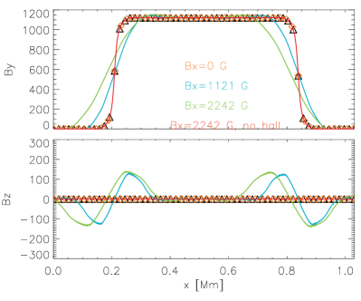
Figure 1: $B_{y}$ (top panel) and $B_{z}$ (bottom panel) as a function of $x$ are shown for the different 1D simulations with constant Hall term at time $t=20$ s. The initial condition is the same for all simulations (shown with black triangles). The runs have different constant $B_{x}$ values: $B_{x}=0$ G (orange diamonds), $B_{x}=1121$ G (blue line), $B_{x}=2242$ G with the Hall term (green line), and $B_{x}=2242$ G without the Hall term (red line). Note that the orange diamonds, red line, and black triangles overlap.

For this test, we set $B_{x}$ constant ($B_{x}=0,1121,2242$ G are shown with orange diamond symbols, and blue and green lines in Figure 1). With higher $B_{x}$, the rate at which $B_{y}$ and $B_{z}$ change with time increases. However, the total magnetic flux should remain the same at all times, since the Hall term cannot convert the magnetic flux into thermal or kinetic energy. Note also that the Hall term will give rise to a non-zero $B_{z}$ (and therefore a non-zero $u_{z}$ in a dynamic simulation) even if the field originally has no component in the $z$-direction. Figure 1 shows $B_{y}$ in the top panel and $B_{z}$ at the bottom panel for four different runs. All cases have the same jump in $B_{y}$ (black triangle symbols in the top panel) and a constant Hall term. In the test shown in red line in Figure 1 does not have the Hall term and $B_{x}=2242$ G. All of these tests are shown at the same instant ($t=20$ s).

The rate of change of $B_{y}$ and $B_{z}$ is as expected, i.e., the case with $B_{x}=2242$ G leads to an increase of unsigned total flux of $B_{z}$ (integrated along the x-axis) that is twice as large as the case where $B_{x}=1121$ G. Moreover, the case $B_{x}=0$ G behaves similarly to the case with no Hall term. The magnetic flux is in all cases conserved. This gives us confidence that our implementation of the Hall term in the code is satisfactory.

2.2.2 1D Ambipolar test

In 1D, the induction equation for $B_{y}$ is:

$$\frac{\partial B_{y}}{\partial t}=\eta_{amb}\frac{\partial}{\partial x}\left(B_{y}^{2}\frac{\partial B_{y}}{\partial x}\right)$$ (27)

Apart from the trivial solution, $B_{y}=constant$, it is clear that Equation 27 also permits a steady solution of the form of $B_{y}\propto x^{1/3}$ (see Brandenburg & Zweibel, 1994, for details). In this expression we should keep in mind that the code includes numerical diffusivity in addition to ambipolar diffusion. We consider the evolution of an initially sinusoidal profile of $B_{y}$. This profile evolves, and strong gradients become stronger approaching the form $B_{y}\propto x^{1/3}$ as time progresses. Figure 2 shows the initial condition of $B_{y}$ (solid line) and at $t=50$ s (dashed line) which is close to the steady solution. Observe that where the gradient of $B_{y}$ is large $B_{y}$ closely follows the expression $B_{y}\propto x^{1/3}$ (dash-dotted line).

Ambipolar diffusion converts magnetic energy into thermal energy as discussed above. In this 1D test, we turn off the heating from artificial diffusion and only allow heating from the ambipolar diffusivity. Such heating in this simple simulation must follow the expression

$$\frac{\partial e}{\partial t}=\eta_{amb}J_{z}^{2}B_{y}^{2}.$$ (28)

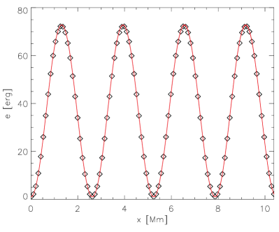
Figure 3: Test of ambipolar diffusion on the energy balance. Energy is shown as a function of $x$ at t=2.1 s. The energy from the model is shown with the black diamonds and the energy extracted from Equation 29 is shown with the red line. Note that the red line is overlapping with the black diamonds.

Figure 3 shows the energy profile with $x$ of this test (black diamonds) at $t=2.1$ s. Calculating the right hand side of this expression using the sinusoidal shape of $B_{y}$ from the initial condition, then deriving $J_{z}$, we calculate the energy to be

$$e=e_{init}+\eta_{amb}J_{z}^{2}B_{y}^{2}\Delta t,$$ (29)

where $\Delta t$ is the time increment. This relationship is shown with the red line in Figure 3. The black diamonds overlaps the red line as would be expected. This indicates we have correctly implemented ambipolar diffusion in the code.

2.2.3 Collision frequencies test: VAL-C model

In order to test whether the absolute values of the diffusion terms are calculated correctly, we use three different sources for the neutral-ion collision frequency ($\nu_{ni}$, see Section 2.1.4). This also allows us to study the uncertainties involved in the various formulas for the collision frequency, as already studied for 1D-static models by De Pontieu et al. (2001). We test our implementation in the Bifrost code by using the densities and temperatures from the VAL-C atmospheric model (Vernazza et al., 1981) which allows us to compare our results with those found in the published literature. Indeed, we correctly obtain the neutral-ion collision frequencies as a function of height as can be seen by comparing our Figure 4 with Figure 2 in De Pontieu et al. (2001). The large dip in the collision frequency at $0.5$ Mm is due to low number of ions (mostly non-hydrogen species) in this region..

2.3 Initial and boundary conditions

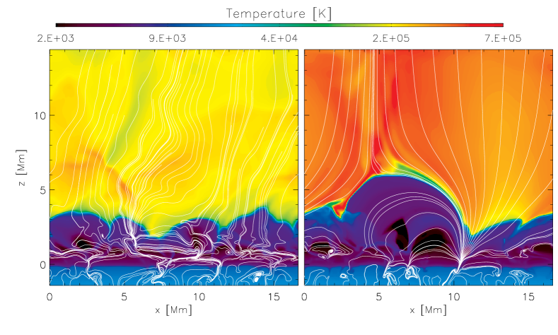
Figure 5: 2D snapshots of the two initial 2.5D MHD models. The initial conditions with weak (simulations labeled WA, WB, and WC) and strong magnetic field (SA, SB, and SC) are shown respectively in the left and right panel. The color scale shows the temperature in logarithmic scale and the magnetic field is shown with white lines.

Let us now consider the importance and validity of the generalized Ohm’s law in a “realistic” 2.5D simulation of the solar atmosphere. The 2.5D computational domain stretches from the upper convection zone to the lower corona and is evaluated on a non-uniform grid of $512\times 325$ points spanning $16\times 16$ Mm². The frame of reference for the model is chosen so that $x$ is the horizontal direction and $z$ is the vertical direction (Figure 5). The grid is non-uniform in the vertical $z$-direction to ensure that the vertical resolution is good enough to resolve the photosphere and the transition region with a grid spacing of $28$ km, while becoming larger at coronal heights where gradients are smaller.

We run two different initial conditions with different values for the unsigned magnetic field strength but with similar field configurations (Figure 5). $B_{y}$ is originally set to zero. The initial model starts with a magnetic field that is inclined some 5 degrees with respect to the vertical axis and the two different setups for the unsigned field strengths in the photosphere are $0.25$ G, the other $90$ G. These two initial conditions are run for the three different formulas that were mentioned above to calculate the collision frequency $\nu_{in}$. The simulations with the initially weak magnetic field using cases A, B or C for the neutral-ion collision frequency are labeled WA, WB or WC, while the strong field simulations using cases A, B, or C for the neutral-ion collision frequency are labeled SA, SB, or SC, respectively. Table 1 list the different simulations.

In the following we will refer in our analysis to simulations WB and SB, unless otherwise noted.

3 Results

The simulations presented include the dynamic processes (including radiative losses) of the photosphere and chromosphere and a self-maintained chromosphere and corona. This is a very different type of model as compared to semi-empirical models such as the VAL-C model, or previous simulations investigating the effects of partial ionization which had a simplified treatment of the energy balance (and ionization degree). It is thus of significant interest to determine how dynamic atmospheres such as from our simulations impact the importance of the ambipolar diffusion and the Hall terms (also assuming different approximations to the collision frequency), and to compare the results with those from the models based on a VAL-C type atmosphere.

The basic structure of our modeled chromospheres are shown in Figure 5. A full description of their properties fall outside the scope of this paper but we will mention the most important as concerns ambipolar diffusion and the Hall term: the basic thermodynamic state of the chromosphere is maintained by the continual injection of acoustic shocks from the photosphere. These perturbations are due to the chaotic generation of waves in the convection zone, of which waves with periods of order $3$ minutes will propagate and steepen in the chromosphere, as is well known and as extensively studied by Carlsson & Stein (1992, 1994). The propagation of waves will be modified in the presence of a magnetic field (Bogdan et al., 2003; De Pontieu et al., 2004; Heggland et al., 2007; McIntosh et al., 2011; Heggland et al., 2011, among others)

but will nevertheless steepen and form strong shocks, with high temperatures in the shock fronts and very low temperatures in the regions behind (Leenaarts et al., 2011). These “cold chromospheric bubbles” can be seen in both panels of Figure 5 which show temperatures as low as $2\,000$ K or lower. In the strong field case the Lorentz force is clearly important, pushing the corona upwards and allowing cool material to exist at great heights, much higher, up to 5 Mm above the photosphere, than that found in semi-empirical models where the maximum chromospheric height is found to be of order 2-2.5 Mm. The distribution of density and temperature with height in dynamical “realistic” simulations is discussed in much greater detail in e.g. Leenaarts et al. (2011).

3.1 Collision frequencies and diffusivities

As mentioned, most studies of the effects of ion-neutral collisions in the chromosphere have been based, in some form, on semi-empirical models (VAL-C or FAL-C models as shown in Figure 4). However, the chromosphere and transition region are clearly highly dynamic, and it is of great importance to know the effects of the neutral-ion interactions in such dynamic atmospheres. First of all, we are interested in studying the relative importance of the different diffusivities in the chromosphere and transition region. Figures 6 and 7 show the Ohmic diffusion, artificial diffusion, Hall term, and ambipolar diffusion from top to bottom and left to right for the simulations WB and SB, respectively.

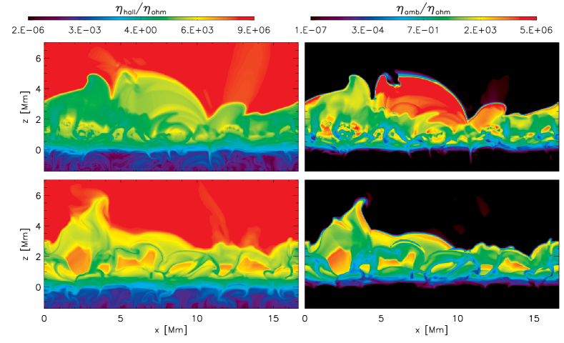
Figure 8: Ratio between the Hall term and Ohmic diffusion (left panels) and ambipolar and Ohmic diffusion (right panels) for the SB simulation (top panels) and WB (bottom panels) at $t=500$ s.

On comparing the different diffusivities, we find that in the entire chromosphere, the Hall term is on average two orders of magnitude larger than Ohmic diffusion. This is true for both simulations WB and SB and is perhaps more easily seen by considering the ratios of the diffusivities plotted in Figure 8. Ambipolar diffusion is roughly four orders of magnitude larger in the weak field (WB) case and fully six orders of magnitude larger than Ohmic diffusion for the strong field SB case. Ambipolar diffusion is considerably larger for SB than for WB because ambipolar diffusion depends quadratically on the magnetic field strength. Note that while Ohmic diffusion has a significant magnitude throughout the atmosphere, ambipolar diffusion is important only in the chromosphere.

Numerical simulations must include some form of artificial diffusion in order to compensate for the fact that they do not have infinite spatial resolution. In the Bifrost code this is done through a so called hyper-diffusivity which in practice means that the diffusion coefficient is increased in regions that require high diffusivity, i.e., where gradients are large. The magnitude of this artificial diffusion is set by the spatial resolution. To some degree this behavior is similar to Ohmic diffusion, but there are also significant differences. Simulations run at the highest possible spatial resolution cannot even come close to the diffusion values found in Ohmic diffusion. This is a well known problem for numerical simulations of the solar atmosphere.

For the simulations reported here, we find an artificial diffusivity in the chromosphere that is three orders of magnitude larger than the Ohmic diffusivity and that is up to five orders of magnitude larger than the Ohmic diffusivity in the corona. By design, the artificial diffusion is largest where the shocks and other high gradient phenomena are located. Moreover, since the grid is non-uniform and the grid resolution decreases with height, artificial diffusion will on average be larger in the corona than in the lower layers. In contrast, the Ohmic diffusion is largest in the upper photosphere and chromosphere. As result of these differences between artificial diffusion and Ohmic diffusion, the magnetic Reynolds number on the Sun and in the simulations is completely different: the magnetic Reynolds number is several orders of magnitude higher in the solar atmosphere than even the highest resolution simulations. Since Ohmic diffusion is negligible compared to artificial diffusion we do not include its effects either in the induction equation nor in the energy equation. In a similar manner, as result of the low resolution of these simulations, the artificial diffusion will mask the Hall term, but here we are interested in describing the stratification of the Hall term and ambipolar diffusion in self-consistent magneto-convection simulations.

One of the most interesting results of our calculations is that, on the other hand, ambipolar diffusion is of the same order or, in some regions, even larger than the artificial diffusion in the chromosphere. This is a perhaps surprising, but crucial property of the chromosphere. It allows us to use our numerical simulations to study the effects of ambipolar diffusion while using the correct physical magnitudes of the coefficients. As a result, the chromosphere may be the only region where simulations are close to reality once all the physics are included in the code, despite the necessarily limited resources of todays computing technology. This has an impact beyond the chromosphere, since it directly affects discussions on whether these self-consistent magneto-convective simulations provide a realistic driver and boundary to the corona. For example, recent simulations by Hansteen et al. (2010) suggest a preponderance of heating in the lower atmosphere (first few Mm above the photosphere), implying that much of the coronal heating occurs towards the footpoints (Martínez-Sykora et al., 2011). The large ambipolar dissipation we find here suggests that such simulations (which only include artificial resistivity) are actually much more realistic than previously thought, including the predictions of heating low down.

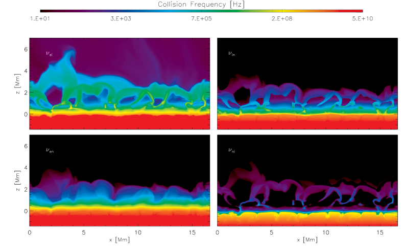
Figure 9: Comparison of the different collision frequencies for the WB simulation at $t=500~{}s$. $\nu_{ei}$, $\nu_{en}$, $\nu_{in}$, and $\nu_{ni}$ are shown from top to bottom and left to right respectively in logarithmic scale.

The Ohmic diffusivity, Hall term, and ambipolar diffusivity depend on the electron density, while the Ohmic and ambipolar diffusivites also depend on collision frequencies which are shown in Figures 9 and 10 for the weak field WB and strong field SB simulations (see Appendix A). (Note that the Ohmic diffusivity is proportional to the collision frequency, while ambipolar diffusivity is inversely proportional to the collision frequency.) On average, the collision frequency between electrons and ions is larger than both the ion-neutral, electron-neutral, and neutral-ion collision frequencies in the chromosphere, in the WB simulation one order of magnitude larger and in the SB simulation two orders of magnitude. This difference in collision frequencies between the WB and SB simulations is mainly because the chromosphere is hotter in the SB simulation as a result of ambipolar heating.

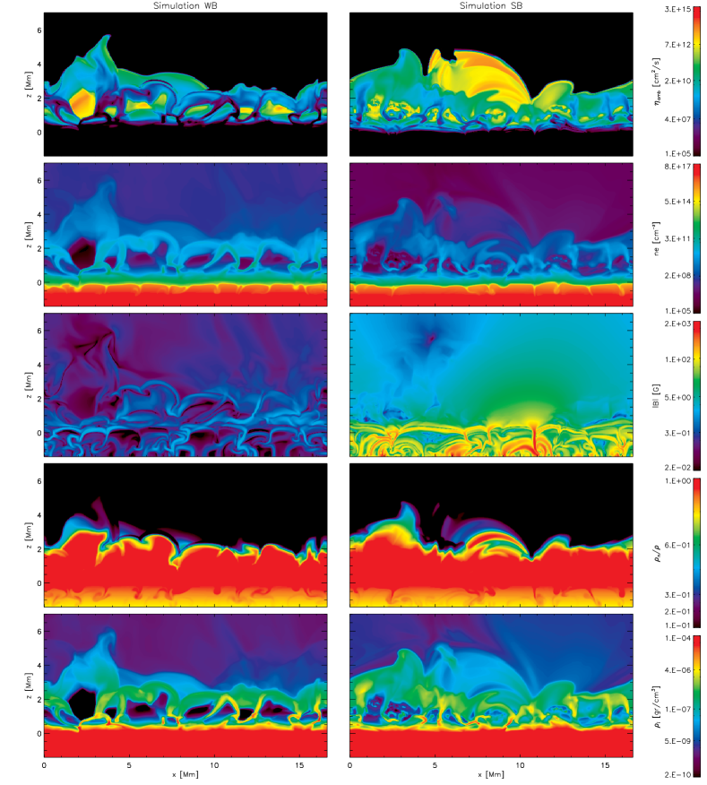
Figure 11: The ambipolar diffusion, electron density, absolute value of the magnetic field, ratio between neutral and total density and ion density are shown from top to bottom for the WB simulation (left panels) and SB (right panels) at $t=500$ s.

The electron-ion collision frequency also shows strong variation throughout the chromosphere, by almost 5 orders of magnitude in both simulations. This variation is due to the electron density variation in the chromosphere (see second row in Figure 11 and Equation 23). As a result, the electron-ion collision frequency is lower inside the cold chromospheric bubbles than in the shock fronts. In the chromosphere, the electron-neutral and ion-neutral collision frequencies are similar in magnitude. However, the ion-neutral collision frequency shows a stronger variation in space in the middle chromosphere than the electron-neutral collision frequency. This is especially true in the cold chromospheric bubbles, where the ion-neutral collision frequency is significantly lower. What causes these differences? First, we note that $\rho_{n}$ shows less variation in horizontal cuts in the lower chromosphere than $\rho_{i}$ because the region is mostly dominated by neutrals. As result of this, the neutral density is almost similar to the total density. In the cold bubbles, hydrogen is mostly neutral, and the only ions are provided by the heavier metals. While both the electron-neutral and ion-neutral collision frequency are dependent on the neutral density (which does not vary much in the lower chromosphere), the dominance of metals in providing ions implies that the average mass per ion increases significantly in the cold bubbles (compared to the rest of the chromosphere). The associated drop of average thermal speed (for the heavy ions compared to protons) is the reason for the sharp drop in ion-neutral collision frequency in the bubbles (compared to the rest of the chromosphere). The neutral-ion collision frequency is even lower than the ion-neutral collision frequency in the bubbles, because there are so few ions available to collide with (bottom panels in Figure 11).

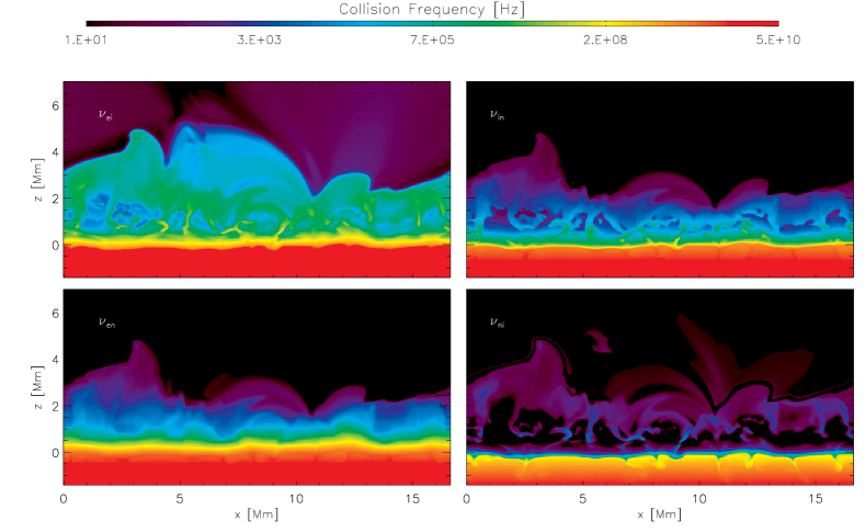
Figure 10: Comparison of the different collision frequencies for the SB simulation at $t=500$ s. The layout is the same as in Figure 9.

We now consider which parameters are responsible for the changes in diffusivities throughout the solar atmosphere. In both simulations (WB and SB), the strongest Ohmic diffusivity is concentrated in the lower-middle chromosphere while it is weaker in the corona and convection zone. In the chromosphere, the Ohmic diffusivity varies over a range of almost four orders of magnitude. This variation in the chromosphere is due to the strong variation of the electron density and collision frequency of electrons with neutrals and ions (Figures 9-11). Ohmic diffusion is large in the expanding cool bubbles and low where temperatures are higher. This is because the Ohmic diffusion variations are dominated by the variations in electron density, which is very low in the cool bubbles, and large in shock fronts. The collision frequency of electrons with ions and neutrals does not drop as precipitously in the cold bubbles since there are plenty of neutrals to collide with in these bubbles.

The Hall term is largest in the lower-middle chromosphere and in the corona (Figure 8). This is because it is inversely proportional to the electron density which is small in both regions. We see that for both simulations, the Hall term is larger than the Ohmic diffusivity in the chromosphere and corona, but not in the photosphere nor in the convection zone. In the cooler regions of the chromosphere, the Hall term is relatively even higher than in the shock fronts, and up to three orders of magnitude greater than the Ohmic diffusivity. Such differences are a bit larger in the WB simulation, since electron density is smaller in the cold chromospheric bubbles in the weak field model. This difference in the electron density between WB and SB is because the cold bubbles have cooler temperatures in WB simulation than in the simulation SB. In the intergranular lanes in the photosphere, the Hall term is the most important diffusion term after the artificial diffusion. Therefore, since the Hall term is proportional to the strength of the magnetic field, this term may be important to consider in magnetoconvective simulations that include strong magnetic fields.

Ambipolar diffusion is important in the region from the upper-photosphere to the upper-chromosphere. In the photosphere, ambipolar diffusion shows some importance in intergranular lanes which have strong concentrations of magnetic field (Figure 11). Therefore, the strong field in the SB simulation shows considerably more diffusivity in intergranules with high magnetic flux concentrations than in the weak field WB simulation. In the chromosphere, ambipolar diffusion dominates almost everywhere except for in the lower chromosphere in shock fronts. The largest difference between ambipolar and Ohmic diffusion is located in the cold chromospheric bubbles and near the upper-chromosphere/lower transition region. Note that for the SB simulation the ratio between ambipolar and Ohmic diffusion is almost four orders of magnitude larger than in the WB simulation due to the quadratic dependence of the ambipolar diffusivity on the magnetic field strength. The ambipolar diffusivity is large in the cold bubbles since the ion density and the ion-neutral collision frequencies are low, but mainly because the ion density is extremely low (5 orders of magnitude lower than in the chromospheric shock fronts). In the upper chromosphere, the ambipolar diffusivity becomes relatively strong due to low densities — which lead to low ion-neutral collision frequencies — but only in those regions where the magnetic field strength is high. In the cold bubbles the ion density is low because of the adiabatic expansion and cooling, whereas in the upper chromosphere, it is because the density drops by 2–3 orders of magnitude compared to the lower chromosphere. As shown in Figure 11, the ambipolar diffusivity depends strongly on the ion and neutral density and thus on the ionization state of the chromospheric plasma. However, it is well known that in the middle and upper chromosphere the ionization and recombination rates are fairly slow for hydrogen which will not be in ionizational equilibrium (Carlsson & Stein, 2002). This suggests that, in order to treat ambipolar diffusion realistically, it is necessary to solve the full time dependent rate equations for hydrogen ionization (Leenaarts et al., 2007).

3.1.1 Comparison with VAL-C model

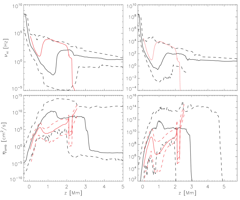
Figure 12: Minimum (dashed line), median (solid line) and maximum (dashed line) of $\nu_{in}$ (top panels) and $\eta_{amb}$ (bottom panels) as function of height are shown for the simulation labeled WB (black in left panels), SB (black in right panels) and for the VAL-C atmosphere (red). The VAL-C ambipolar diffusion is calculated taking into account the maximum, minimum and median magnetic field of the 2D models as a function of height. The minimum, median and maximum are calculated in horizontal planes for the instant $t=500$ s.

The VAL-C model does not provide a good description of the strong temporal and spatial variations found in the physical variables of the chromosphere. In the section above, we have seen that the different collision frequencies and diffusivities show spatial variations of several orders of magnitude at the same height in the chromosphere. The lower-chromosphere changes rapidly due to the shock fronts; these lead to changes in the thermodynamic structure of the lower chromosphere on times-scales shorter than a minute. As a result of this, cold chromospheric bubbles appear and disappear in minutes. Due to the ambipolar diffusion, plasma is heated in the cold bubbles on timescales shorter than those characterizing the shock front. As a result of the spatial and temporal variations, the neutral-ion collision frequency varies by almost eight orders of magnitude in the chromosphere in the 2D simulation, whereas the VAL-C model has a unique value for the collision frequency at every height (Figure 12). In the cold chromospheric bubbles, the collision frequency drops to considerably lower values than those found in the VAL-C model. This is a result of the low ion number density in these areas, which are overestimated in the VAL-C model.

We use the maximum, minimum and median magnetic field of the 2D models (SB and WB) as a function of height in order to calculate the range of ambipolar diffusivities in the semi-empirical VAL-C model. The ambipolar diffusion has a very wide range of values, 8 orders of magnitude in simulation SB and 11 orders of magnitude for simulation WB. These variations are almost 6 or 8 orders of magnitude larger than in the VAL-C model. The ambipolar diffusivity in the 2D simulations is much higher in most of the chromosphere compared to what is found in the VAL-C model. The reason for the large difference of the neutral-ion collision frequency and the ambipolar diffusivity in the VAL-C model (compared to the 2D model) is because the VAL-C model does not capture the thermodynamics of the cold chromospheric bubbles where the neutral-ion collision frequency drops precipitously.

These large differences in both the neutral-ion collision frequency and ambipolar diffusivities, found between the VAL-C model and our simulation should lead to a re-examination of previous results related to the generalized Ohm’s law (see references) using semi-empirical models to define the density and temperature structure. We also reiterate the importance of taking into account the likely dynamic state of hydrogen ionization (Leenaarts et al., 2007).

3.1.2 Other methods to calculate collision frequencies

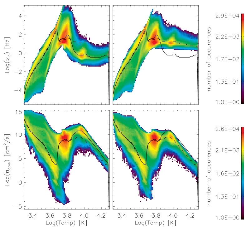
Figure 13: Joint probability distribution function (JPDF) of the temperature against of the ion-neutral collision frequency (top) and ambipolar diffusivity (bottom) for the simulations labeled WB (left) and WC (right). JPDF is calculated integrated over 220 s above the photosphere. The colorbar is in logarithmic scale. The median as a function of temperature for the WB and WC cases are shown in solid, and dashed lines respectively.

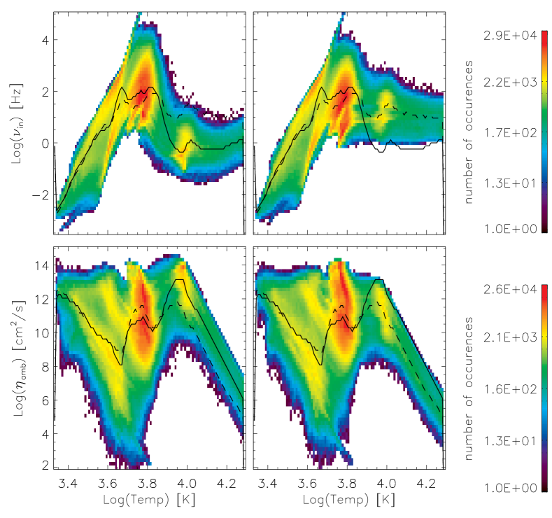
Figure 14: The layout is the same as Figure 13. However, the simulations are SB (left) and SC (right).

We considered three different methods to calculate $\nu_{in}$ (Section 2.1.4), and thus, the ambipolar diffusivity. Do the different methods give similar values of the collision frequency and/or diffusion for the different models? We note that the evolution of the simulations using the different methods to calculate the collision frequency (WA, WB and WC, and SA, SB, and SC) diverge within a few minutes. We therefore integrate the properties of the models in time in order to study the different values of the collision frequency and ambipolar diffusion, and proceed as follows. In Figure 13 we show the joint probability distribution function (JPDF) of the temperature versus the ion-neutral collision frequency (top) and the ambipolar diffusivity (bottom) for the simulations labeled WB (left) and WC (right). In Figure 14 we show the cases SB and SC in a similar manner. We have integrated over 4 minutes. Note that the variation of the $y$-axes are logarithmic and cover more than 10 orders of magnitude. We mostly focus on cases B and C since those are the most recent, and include more advanced calculations of the collision frequencies.

The values for $\nu_{in}$ and $\eta_{amb}$ differ in range and mean values for the different cases in each simulation. These differences are significant in certain temperature ranges. The differences between the different methods to calculate the ion-neutral collision frequency are similar for both atmospheres (weak and strong magnetic field strength). For instance, at $\log(T)\approx 3.7$ ($5000$ K), case B shows ion-neutral collision frequencies that are a factor two larger than for case C. At temperatures larger than $\log(T)\approx 3.7$, the collision frequency for case B is almost two orders of magnitude smaller than in case C. As a result, in certain temperature ranges, the largest values of the ambipolar diffusion for case B are almost 2 orders of magnitude larger than for case C. For temperatures lower than $\log(T)\approx 3.6$ ($4000$ K), the median collision frequency as a function of temperature is roughly similar between cases B and C, but not the distribution, as can be seen: case B reaches collision frequencies smaller than case C.

At temperatures larger than $\log(T)\approx 3.8$ ($6300$ K), the collision frequencies for case C are one order of magnitude larger than for case B. As a result, the median of the ambipolar diffusion for cases WC and SC is one order of magnitude smaller than for WB and SB.

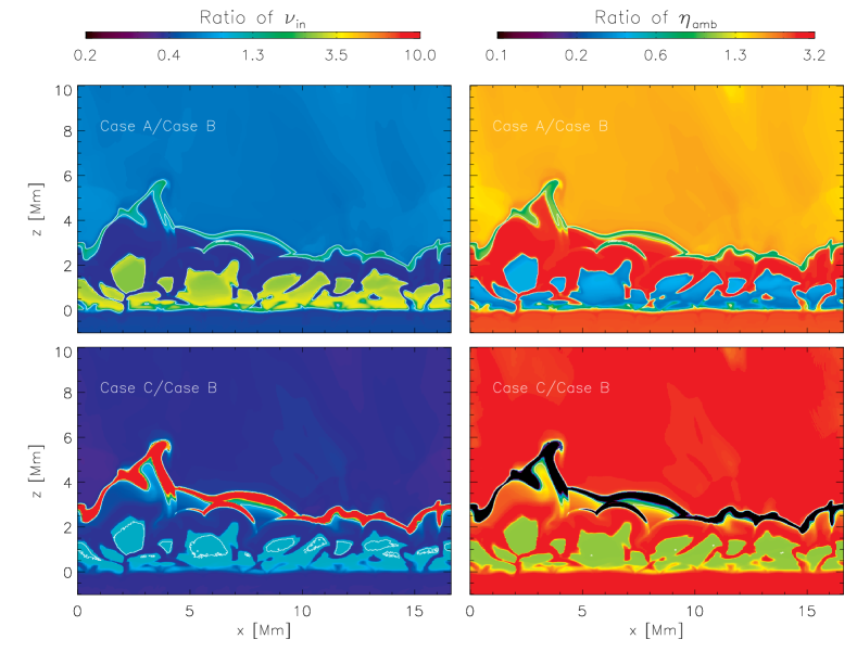
Figure 15: Ratio of the ion-neutral collision frequency (left panels) and ambipolar diffusivity (right panels) between case A to case B (top panels) and case C to case B (bottom panels), for the atmosphere with weak magnetic field strength. The white contours show where these ratios are equal to one. Note that the color scheme is in a logarithmic scale. We used the same atmospheric model for all three cases, i.e., before the simulations diverge with time, but then calculated the collision frequency and ambipolar diffusion using the different formulas of each case.

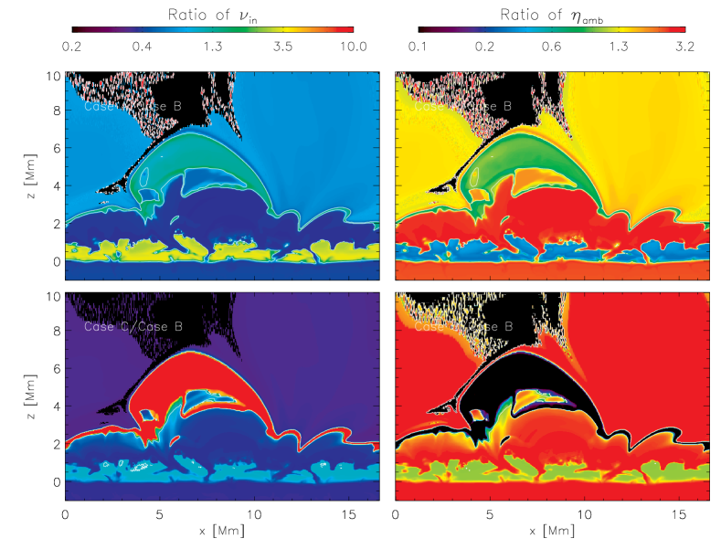
Figure 16: Same as Figure 15 for the atmosphere with strong magnetic field.

In order to have a better impression where in the atmosphere the ion-neutral collision frequency and ambipolar diffusion differ between the different cases, we take the same atmospheric model (simulation WB or SB at $t=2500$ s) and calculate from these two models the collision frequency and ambipolar diffusivity using the different methods (Figures 15-16). It is interesting and important to see that at the precise location where the ambipolar diffusion is really high (in cold chromospheric bubbles and in the upper chromosphere), the different methods differ most. In the cold chromospheric bubbles for both atmospheres (weak and strong magnetic field), the collision frequency using case B is almost 4 times smaller than case A, but similar to case C. As result, the ambipolar diffusivity is more than 2 times smaller using the method of case B than for case A. In the upper chromosphere or shock fronts, the collision frequency using case B is almost two times larger than case A and slightly larger than with case C. As a result, the ambipolar diffusivity using case B is more than 3 times smaller than case A, and almost 3 times smaller than case C. However, in the proximity of the transition region, the collision frequency for case B is a bit smaller than case A, and more than 10 times smaller than case C. As result of this, the ambipolar diffusivity using case B is a bit larger than case A, and more than 10 times larger than case C.

These large differences between each method are due to the different temperature dependences (see Appendix A). As mentioned, these differences lead to rapidly diverging thermodynamic evolution in the various models. Thus, it is important to take into account this uncertainty in calculating the collision frequencies when the generalized Ohm’s law is modeled.

3.2 Approximations to the generalized Ohm’s law

The generalized Ohm’s law is based on several approximations and considerations. In this section we describe where these approximations fail and the implications of this failure. We employ the atmospheres of the WB and SB simulations in this discussion.

3.2.1 Approximations in the momentum equation

Let us establish and validate the different assumptions underlying the generalized Ohm’s law as implemented in the code, and see if they are fulfilled in the fully dynamic self-consistent simulations. One of the first consideration is that the ion density dominates over the electron density ($\rho_{i}/\rho>>\rho_{e}/\rho$). Everywhere in the atmosphere, the values of ion and electron densities remain within the range that fulfill $\rho_{i}/\rho>>\rho_{e}/\rho$ so that electron inertia can be neglected.

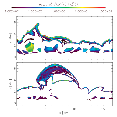
Figure 17: The drift momentum has to be smaller than the fast momentum (Equation 6). The ratio between both terms, i.e., $\rho_{i}\rho_{n}{\bf u_{D}^{2}}$ and $\rho^{2}(v_{a}^{2}+c_{s}^{2})$ is shown for the simulations labeled WB (top panel) and SB (bottom panel) at $t=500$ s. The colorbar is in logarithmic scale and it is the same for both panels.

In order to neglect the effects of drift momentum in the momentum equation, the drift momentum has to be smaller than the fast momentum ($\rho\sqrt{v_{a}^{2}+c_{s}^{2}}$, see Equation 6 and Pandey & Wardle (2008)). This approximation is fulfilled in most of the atmosphere under both strong and weak field conditions. The only exception is in the weak field atmosphere, where some low density areas just below the transition region show a ratio of order 0.1-1 (see Figure 17). This is because the ion-neutral collision frequency drops significantly there, so that the drift between ions and neutrals becomes rather large. As a result, in these small regions the plasma becomes decoupled from the neutrals, and it may be necessary to add the drift momentum to the momentum equation, and/or solve the MHD equations using multiple fluids. In the weak field atmosphere, a few of the cold, expanding bubbles show ratios of order 0.1, so that the fast momentum does stay in excess of the drift momentum. This suggests that the region below the transition region is the only one of concern for this particular condition.

3.2.2 Approximations in the induction equation

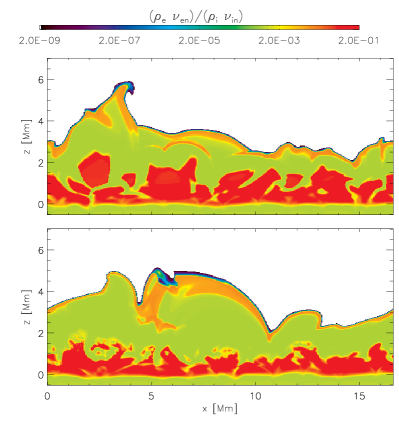
Figure 18: Following the Equation 16, the ratio between $\rho_{e}\nu_{en}$ and $\rho_{i}\nu_{in}$ is shown for the simulations labeled WB (top panel) and SB (bottom panel) at $t=500$ s. The colorbar is the same for both panels and it is in logarithmic scale.

To allow the removal of the time dependence of the drift momentum equation (Pandey & Wardle, 2008), the electron density times the collision frequency of electrons with neutrals has to be smaller than the ion density times the collision frequency of ions with neutrals ( $\rho_{e}\nu_{en}<<\rho_{i}\nu_{in}$). This approximation is fulfilled in most of the atmosphere with the exception of some areas in the upper photosphere and in the cold chromospheric bubbles (Figure 18). In the cold bubbles, the electron-neutral collision frequency is almost similar to the ion-neutral collision frequency. In the upper photosphere, and the collision frequency of electrons with neutrals is relatively large so $\rho_{e}\nu_{en}<<\rho_{i}\nu_{in}$ is not fulfilled. Therefore, in these regions, the proper way to solve the ambipolar term in the induction equation is by calculating the drift velocity using the fully time dependent equation of ${\bf u_{D}}$ (Pandey & Wardle, 2008).

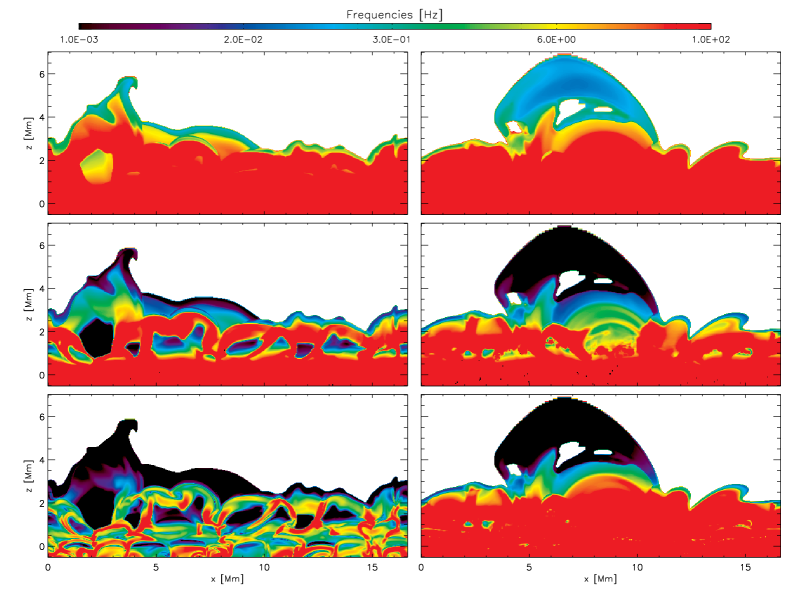
Figure 19: A study of the validity of the assumptions underlying the generalized Ohm’s law. The dynamic frequency of the simulations ($\approx 0.5$ Hz) should remain lower than the frequency limits shown in the different panels for simulations WB (left panels) and SB (right panels) at $t=500~{}s$. The frequencies are following the expressions Equation 18 (top panels), Equation 7 (middle panels) and Equation 19 (bottom panels). The colorbar for each frequency is located at the top side and is in logarithmic scales. The white color is where the temperature is above $3\,10^{4}$K.

Some of the approximations used in deriving the equations require that the dynamical frequency remains smaller than the frequencies shown in Figure 19. The typical timescales on which the simulated atmosphere evolves is of order 10s or longer, i.e., a dynamic frequency of $\approx 0.5$ Hz or lower: if the frequencies shown in Figure 19 are higher than $\approx 0.5$ Hz, the assumptions underlying the generalized Ohm’s law are fulfilled.

The first assumption is that the time derivative of the drift velocity can be neglected. Following Equation 18, this can be done only if the dynamical frequency is smaller than the frequency $(\rho/\rho_{i})\nu_{ni}$ shown in the top panels of Figure 19. The latter frequency is very high in the upper photosphere and the chromosphere, and stay well above the dynamical frequency of our simulations ($\approx 0.5$ Hz). Only in the vicinity of the transition region does $(\rho/\rho_{i})\nu_{ni}$ become small enough that it is of the same order as the dynamical frequency of the simulations. As a result, we may need to take into account the derivative terms shown in Equation 17 only in this small region in the vicinity of the transition region.

A second assumption is that the dyadic product of the drift velocity in the momentum equation can be neglected (Pandey & Wardle, 2008). This term can only be neglected if the dynamic frequency stays well below the frequency defined in Equation 7 and shown in the middle panels in Figure 19. We find that in the cold chromospheric bubbles (in the weak field case) and in the upper chromosphere (in both weak and strong field cases), this assumption sometimes fails. In these regions, we may thus need to take into account the momentum drift term in the momentum equation.

A final assumption is that the terms of the form $\nabla P\times{\bf B}$ in the induction equation can be neglected. This can only be done when the dynamic frequency stays below the frequency defined in Equation 19 and shown in the bottom panels in Figure 19. This bound for the dynamical frequency strongly depends on magnetic field strength of the model. We find that for the weakly magnetic atmosphere case (WB) this limit is low, and the assumption fails in the upper chromosphere and cold bubbles.In the strongly magnetic atmosphere (SB) the assumptions only fails in the upper part of the chromosphere.

In summary, for the weak field atmosphere we cannot neglect the time derivative and dyadic product of the drift velocity, and the $\nabla P\times{\bf B}$ terms (in the momentum and induction equation respectively) in the cold bubbles and just below the transition region. In all other regions in the weak field atmosphere, the assumptions underlying the generalized Ohm’s law are fulfilled.

For the strong field atmosphere, the generalized Ohm’s law works well in most of the chromosphere, except in the region just below the transition region where the time derivative and dyadic product of the drift velocity and the $\nabla P\times{\bf B}$ terms cannot be neglected.

4 Discussion and Conclusions

We have implemented the partial ionization effects in the Bifrost code in the form of the Hall term and ambipolar diffusion. The code has been tested and verified with different tests that are presented in this paper. The code allows the simulation of the solar atmosphere, from the upper convection zone to the lower corona, with a magnetoconvective photosphere, and a fully-dynamic and self-maintained chromosphere and corona. We studied the different diffusivities in two different models, one is weakly magnetic, and the other is rather strongly magnetic. The magnetic field strength of the latter model is similar to that found in the quiet sun, including the network.

In short, the Ohmic diffusion is roughly three orders of magnitude smaller than the Hall term in the chromosphere, and the latter is three orders of magnitude smaller than the artificial diffusion. Unlike Ohmic diffusion, the Hall term depends on the magnetic field, as does ambipolar diffusion which is strongly dependent on the magnetic field strength. As a result of this, the ambipolar diffusivity is clearly different for the two models; in regions with large ambipolar diffusivity we find it is of the same order as the artificial diffusion in the chromosphere for the weakly magnetic model (WB), and more than one order of magnitude larger than the artificial diffusivity for the strongly magnetic model (SB). The fact that the artificial diffusivity is actually smaller than the ambipolar diffusivity under many chromospheric conditions has some very important consequences. It means that these simulations are capable of providing a surprisingly realistic view of the consequences of the ambipolar diffusion in the chromosphere and corona. This has an impact beyond the chromosphere, since it directly affects discussions on whether these self-consistent magneto-convective simulations provide a realistic driver and boundary to the corona. These results will be described in detail in a follow up paper.

Another important result is that both, the Hall term and ambipolar diffusivity, vary by several orders of magnitude in the chromosphere as result of the time varying dynamics and the strong variations in temperature, electron, ion and neutral density, and magnetic field strength in this region. This strong variation is not taken into account in any of the previous studies which use either 1D semi-empirical VAL-C type models, or lack more sophisticated approaches to the radiation, ionization and energy balance. The largest values of the ambipolar diffusivity are located in the cold chromospheric bubbles that have low temperatures due to strong adiabatic expansion, and in the upper chromosphere because the neutral-ion collision frequency is small. However, the ambipolar diffusion is strongly dependent on the ionization degree, and as shown by Leenaarts et al. (2007), time dependent hydrogen will change the ratio between neutrals and ions compared to LTE conditions. The Bifrost code can treat the time-dependent ionization of hydrogen and we plan to run new simulations taking into account both the generalized Ohm’s law and time-dependent hydrogen ionization.

We have compared different methods to calculate the collision frequency between neutrals and ions. Both the ion-neutral collision frequency and ambipolar diffusivity differ considerably as a function of the method used to calculate this collision frequency. Since ambipolar diffusion has a significant impact on the thermodynamic evolution of these models, the simulations rapidly diverge. When comparing each method we find the largest differences are located in regions where the ambipolar diffusivity is large: in the cold chromospheric bubbles and in the upper chromosphere in the vicinity of the transition region. These differences bring a new uncertainty to the results (Section 3.1.2), and highlight the need for a detailed consideration of the relevant collisional processes in the chromosphere.

Finally, we investigated the different approximations underlying the generalized Ohm’s law as described in detail by Pandey & Wardle (2008). In both models, most of the simplifications are applicable with some exceptions. In the upper-chromosphere the collision frequency is too low, as a consequence, the velocity drift can be large. Therefore, we may need to define the velocity drift and add an extra term in the momentum equation related to the momentum drift between ions and neutrals. In the upper photosphere, and in cold chromospheric bubbles the ambipolar term in the induction equation may need to be calculated using the drift velocity. Moreover, the drift velocity should be calculated using the time dependent form (as shown in Pandey & Wardle, 2008). This is necessary because the ion density and the ion-neutrals collision frequency drop in these cold areas as opposed to the electron density and the electron-neutral collision frequency.

5 Acknowledgments

The 2D simulations have been run with the Njord and Stallo cluster from the Notur project, and the Pleiades cluster through computing grants SMD-07-0434, SMD-08-0743, SMD-09-1128, SMD-09-1336, SMD-10-1622, SMD-10-1869, SMD- 11-2312, and SMD-11-2752 from the High End Computing (HEC) division of NASA. We thankfully acknowledge the computer and supercomputer resources of the Research Council of Norway through grant 170935/V30 and through grants of computing time from the Programme for Supercomputing. This work has benefited from discussions at the International Space Science Institute (ISSI) meeting on “Heating of the magnetized chromosphere” from 21-24 February, 2012, where many aspects of this paper were discussed with other colleagues. To analyze the data we have used IDL. B.D.P. was supported through NASA grants NNX08BA99G, NNX08AH45G and NNX11AN98G.

Appendix A Collision frequencies

In order to calculate the collision frequency between ions and neutral particles we use three different approximations (following the approach by De Pontieu et al. 2001): one described by Osterbrock (1961) (hereafter case A), one described by von Steiger & Geiss (1989) (hereafter case B) and one by Fontenla et al. (1993) (hereafter case C).

As a first approach (case A), we take the formulas from Osterbrock (1961) and De Pontieu & Haerendel (1998), where the collision frequency between neutral hydrogen and protons ($\nu_{Hp}$) are given by:

$$\nu_{Hp}=5\,10^{-19}\sqrt{\frac{1}{2}}\sqrt{\frac{8kT}{\pi m_{H}}}n_{p}$$ (A1)

$m_{H}$ is the hydrogen atom mass, and $n_{p}$ is the proton number density. Note that De Pontieu et al. (2001) had a typo with a factor of 2. The collision frequency ($\nu_{Hm}$) of neutral hydrogen with an ionized metal is defined as:

$$\nu_{Hm}=8\,10^{-20}\sqrt{\frac{m_{m}}{m_{m}+1}}\sqrt{\frac{8kT}{\pi m_{H}}}n_{m}$$ (A2)

where $m_{m}$ and $n_{m}$ are the atomic mass number of metals ions and the number density of metals ions of type $m$, respectively. The collisions between neutral helium and ions is given by:

$$\nu_{Hep}=4\,10^{-20}\sqrt{\frac{1}{5}}\sqrt{\frac{8kT}{\pi m_{H}}}n_{p}$$ (A3)

$$\nu_{Hep}=4\,10^{-20}\sqrt{\frac{m_{m}}{m_{m}+1}}\sqrt{\frac{8kT}{\pi m_{H}}}n_{m}$$ (A4)

For the second approach (Case B), following De Pontieu et al. (2001), von Steiger & Geiss (1989) describe the collision rate as follows:

$$\nu_{Hp}=118\sqrt{\frac{T}{10^{4}}}\left(1-0.125\log{\frac{T}{10^{4}}}\right)^{2}\frac{n_{p}}{10^{16}}$$ (A5)

$$\nu_{Hm}=21.05\sqrt{\frac{A_{m}}{A_{m}+1}}Z_{m}\frac{n_{m}}{10^{16}}$$ (A6)

For the helium-proton and helium-metal collision frequency we follow Geiss & Buergi (1986):

$$\nu_{Hep}=2.2\frac{n_{p}/10^{6}}{\sqrt{T/10^{4}}}Z_{m}$$ (A7)

$$\nu_{Hem}=5.84\sqrt{\frac{A_{m}}{A_{m}+1}}Z_{m}\frac{n_{m}}{10^{16}}$$ (A8)

where $Z_{m}$ is the ionization weight and we considered that the ions have only one ionization state, i.e., $Z_{m}=1$. Note that De Pontieu et al. (2001) have a typo where the expression for $\nu_{Hep}$ is missing the square root symbol for the temperature and the constant $2.2$ is also different.

Finally, we find the collision frequencies for the Case C in the appendix of Fontenla et al. (1993).

Using these collision frequencies (Eq. A1-A8), the collision frequency of neutral Hydrogen with all ions is given by:

$$\nu_{Hi} = \nu_{Hp}+\nu_{HC}+\nu_{HN}+\nu_{HO}+\nu_{HNe}+\nu_{HNa}+\nu_{HMg}+\nu_{HAl}$$ (A10)

$$+\nu_{HSi}+\nu_{HS}+\nu_{HK}+\nu_{HCa}+\nu_{HCr}+\nu_{HFe}+\nu_{HNi}$$

and similarly for the collision frequency of neutral Helium with all ions. Finally, the average neutral-ion collision frequency is given by

$$\nu_{ni}=\frac{\rho_{H}}{\rho_{n}}\nu_{Hi}+\frac{\rho_{He}}{\rho_{n}}\nu_{Hei}$$ (A11)

Note that in the main text we often use $\nu_{in}$, which can be derived from $\nu_{ni}$ using momentum conservation ($\rho_{j}\nu_{jk}=\rho_{k}\nu_{kj}$).

Figure 2: From the ambipolar test, $B_{y}$ is shown as a function of $x$ at t=50 s. The initial condition is shown in solid line. The dashed line shows $B_{y}$ at $t=50$ s. The dash dotted line shows a function proportional to $x^{1/3}$ which is what would be expected from the analytical considerations.

Figure 4: Neutral-ion collision frequency as a function of height for the quiet sun model of Vernazza et al. (1981), using different formulas for $\nu_{ni}$: the dotted line is case A, solid line is case B and dashed line is case C.

Figure 6: Comparison of the different diffusivity terms for the simulation WB at $t=500~{}s$. $\eta_{ohm}$, $\eta_{art}$, $\eta_{hall}$, and $\eta_{amb}$ are shown from top to bottom and left to right respectively in logarithmic scale. Note that more than 9 orders of magnitude are shown.

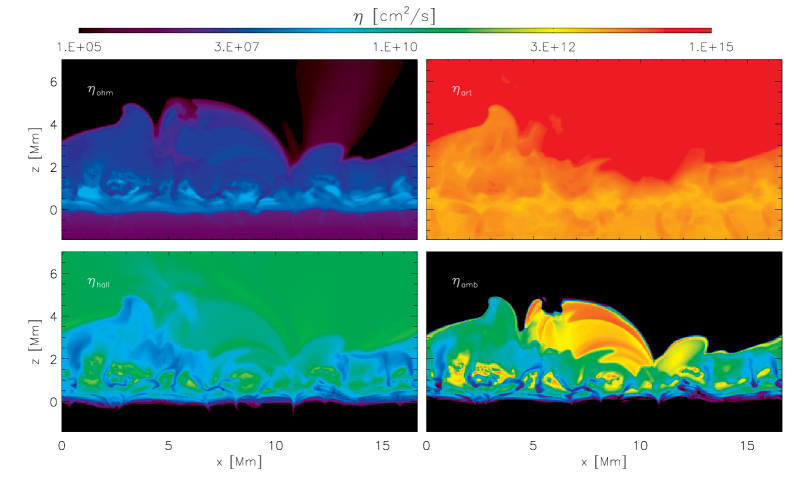
Figure 7: Comparison of the different diffusivities for the simulation SB at $t=500$ s. The layout is the same as in Figure 6.

Table 1: Simulation description

Name	Collision frequency	Min/Mean/Max $|B|$ [G]
WA	Case A	0.003/0.25/3
WB	Case B	0.003/0.25/3
WC	Case C	0.003/0.25/3
SA	Case A	0.1/90/920
SB	Case B	0.1/90/920
SC	Case C	0.1/90/920

Note. — The left column lists the names of the different 2D simulations, middle column lists the method used to calculate the collision frequency between ions and neutrals. The last column shows the minimum, mean and maximum value of the unsigned magnetic field strength in the photosphere.

Table 2: Atomic info

name	H	He	C	N	O	Ne	Na	Mg
abund	12.	11.	8.55	7.93	8.77	8.51	6.18	7.48
mass ion	1.008	4.003	12.01	14.01	16.	20.18	23.	24.32
$X_{i}$	13.595	24.58	11.256	14.529	13.614	21.559	5.138	7.644
name	Al	Si	S	K	Ca	Cr	Fe	Ni
abund	6.4	7.55	7.21	5.05	6.33	5.47	7.5	5.08
mass ion	26.97	28.06	32.06	39.1	40.08	52.01	55.85	58.69
$X_{i}$	5.984	8.149	10.357	4.339	6.111	6.763	7.896	7.633

Note. — The atomic species, abundances ($\log$ of number of atoms per $10^{12}$ Hydrogen atoms), mass ion (uma), and ionization fraction (eV) of the 16 most important atomic species in the solar atmosphere are listed from the top to the bottom row. The various collision frequencies and the electron density are calculated taking into account the atomic species in this table.

References

- Arber et al. (2007) Arber T. D., Haynes M., Leake J. E., 2007, ApJ, 666, 541
- Bogdan et al. (2003) Bogdan T. J., Carlsson M., Hansteen V. H., et al., 2003, ApJ, 599, 626
- Brandenburg & Zweibel (1994) Brandenburg A., Zweibel E. G., 1994, ApJ, 427, L91
- Carlsson & Leenaarts (2012) Carlsson M., Leenaarts J., 2012, ArXiv e-prints, in press in ApJ
- Carlsson & Stein (1992) Carlsson M., Stein R. F., 1992, ApJ, 397, L59
- Carlsson & Stein (1994) Carlsson M., Stein R. F., 1994, Radiation shock dynamics in the solar chromosphere - results of numerical simulations, en Carlsson M. (ed.), Chromospheric Dynamics, p. 47
- Carlsson & Stein (1997) Carlsson M., Stein R. F., 1997, ApJ, 481, 500
- Carlsson & Stein (2002) Carlsson M., Stein R. F., 2002, ApJ, 572, 626
- Cheung & Cameron (2012) Cheung M. C. M., Cameron R. H., 2012, ArXiv e-prints, in press
- Courant et al. (1928) Courant R., Friedrichs K., Lewy H., 1928, Mathematische Annalen, 100, 32, Über die partiellen Differenzengleichungen der mathematischen Physik
- Cowling (1957) Cowling T. G., 1957, Magnetohydrodinamics. Interscience tracts on physics and astronomy
- De Pontieu (1999) De Pontieu B., 1999, A&A, 347, 696
- De Pontieu et al. (2004) De Pontieu B., Erdélyi R., James S. P., 2004, Nature, 430, 536
- De Pontieu & Haerendel (1998) De Pontieu B., Haerendel G., 1998, A&A, 338, 729
- De Pontieu et al. (2001) De Pontieu B., Martens P. C. H., Hudson H. S., 2001, ApJ, 558, 859
- Erdélyi & James (2004) Erdélyi R., James S. P., 2004, A&A, 427, 1055
- Fontenla et al. (1990) Fontenla J. M., Avrett E. H., Loeser R., 1990, ApJ, 355, 700
- Fontenla et al. (1993) Fontenla J. M., Avrett E. H., Loeser R., 1993, ApJ, 406, 319
- Geiss & Buergi (1986) Geiss J., Buergi A., 1986, A&A, 159, 1
- Goodman (2000) Goodman M. L., 2000, ApJ, 533, 501
- Gudiksen et al. (2011) Gudiksen B. V., Carlsson M., Hansteen V. H., et al., 2011, A&A, 531, A154
- Hansteen et al. (2010) Hansteen V. H., Hara H., De Pontieu B., Carlsson M., 2010, ApJ, 718, 1070
- Heggland et al. (2007) Heggland L., De Pontieu B., Hansteen V. H., 2007, ApJ, 666, 1277
- Heggland et al. (2011) Heggland L., Hansteen V. H., De Pontieu B., Carlsson M., 2011, ApJ, 743, 142
- Hyman et al. (1979) Hyman J., Vichnevtsky R., Stepleman R., 1979, Adv. in Comp. Meth, PDE’s-III, 313
- James & Erdélyi (2002) James S. P., Erdélyi R., 2002, A&A, 393, L11
- James et al. (2003) James S. P., Erdélyi R., De Pontieu B., 2003, A&A, 406, 715
- Khodachenko et al. (2004) Khodachenko M. L., Arber T. D., Rucker H. O., Hanslmeier A., 2004, A&A, 422, 1073
- Khodachenko et al. (2006) Khodachenko M. L., Rucker H. O., Oliver R., Arber T. D., Hanslmeier A., 2006, Advances in Space Research, 37, 447