Detection of Semi-Major Axis Drifts in 54 Near-Earth Asteroids: New Measurements of the Yarkovsky Effect

Abstract

We have identified and quantified semi-major axis drifts in Near-Earth Asteroids (NEAs) by performing orbital fits to optical and radar astrometry of all numbered NEAs. We focus on a subset of 54 NEAs that exhibit some of the most reliable and strongest drift rates. Our selection criteria include a Yarkovsky sensitivity metric that quantifies the detectability of semi-major axis drift in any given data set, a signal-to-noise metric, and orbital coverage requirements. In 42 cases, the observed drifts ($\sim 10^{-3}$ AU/Myr) agree well with numerical estimates of Yarkovsky drifts. This agreement suggests that the Yarkovsky effect is the dominant non-gravitational process affecting these orbits, and allows us to derive constraints on asteroid physical properties. In 12 cases, the drifts exceed nominal Yarkovsky predictions, which could be due to inaccuracies in our knowledge of physical properties, faulty astrometry, or modeling errors. If these high rates cannot be ruled out by further observations or improvements in modeling, they would be indicative of the presence of an additional non-gravitational force, such as that resulting from a loss of mass of order a kilogram per second. We define the Yarkovsky efficiency $f_{Y}$ as the ratio of the change in orbital energy to incident solar radiation energy, and we find that typical Yarkovsky efficiencies are $\sim$10^-5.

1 Introduction

Understanding how the Yarkovsky force modifies asteroid orbits has illuminated how asteroids and meteorites are transported to near-Earth space from the main belt and has allowed for deeper understanding of the structure of asteroid families (Bottke et al., 2006). The Yarkovsky force is necessary for accurately predicting asteroid trajectories, including those of potentially hazardous asteroids (Giorgini et al., 2002; Chesley, 2006; Giorgini et al., 2008; Milani et al., 2009).

The Yarkovsky effect (or force) describes the process by which an asteroid’s surface thermal lag and rotation result in net thermal emission that is not aligned towards the Sun (Bottke et al., 2002b, 2006). The so-called diurnal component of the Yarkovsky effect operates as follows. A prograde-spinning object generally has a component of this surface thermal emission anti-aligned with the motion along the orbit, producing a net increase in the object’s semi-major axis (i.e., $da/dt>0$, where $a$ is the semi-major axis). Conversely, a retrograde-spinning object generally has a component aligned with its velocity, shortening its semi-major axis (i.e., $da/dt<0$).

The maximum possible drift rate for any radiation-powered force acting on near-Earth asteroids (NEAs) can be obtained by equating the incident solar radiation energy in a given time interval to the change in orbital energy during the same interval. We find

$$\frac{da}{dt}=f_{Y}\frac{3}{4\pi}\frac{1}{\sqrt{1-e^{2}}}\frac{L_{\odot}}{GM_{\odot}}\frac{1}{D\rho},$$ (1)

where $f_{Y}$ is an efficiency factor analogous to that used by Goldreich & Sari (2009), $e$ is the eccentricity, $L_{\odot}$ and $M_{\odot}$ are the luminosity and mass of the Sun, $G$ is the gravitational constant, and $D$ and $\rho$ are the effective diameter and bulk density of the asteroid. This equation exhibits the expected dependence on the asteroid area-to-mass ratio. In convenient units, it reads

$$\frac{da}{dt}=\frac{1.457}{\sqrt{1-e^{2}}}\left(\frac{f_{Y}}{10^{-5}}\right)\left(\frac{1\ {\rm km}}{D}\right)\left(\frac{1000\ {\rm kg\ m}^{-3}}{\rho}\right)10^{-3}{\rm AU/Myr}.$$ (2)

Maximum efficiency ($f_{Y}$=1) would convert all incoming solar radiation into a change in orbital energy. We will show in Section 3 that typical Yarkovsky efficiencies are $f_{Y}\sim 10^{-5}$, and that typical rates are $\sim 10^{-3}$AU/Myr for kilometer-sized asteroids. The low efficiency and rates are due to the fact that it is the momentum of departing thermal photons that moves the asteroid.

Chesley et al. (2003) used precise radar ranging measurements to (6489) Golevka and reported the first detection of asteroidal Yarkovsky drift. The drift rate for this NEA of $da/dt=(-6.39\pm 0.44)\times 10^{-4}$ AU/Myr (Chesley et al., 2008) corresponds to an efficiency $f_{Y}=5\times 10^{-6}$ for $D$=530 m and $\rho=2700$ kg m^-3.

Vokrouhlický et al. (2008) employed the Yarkovsky effect to link a 1950 observation to asteroid (152563) 1992 BF with a $da/dt$ rate of $(-10.7\pm 0.7)\times 10^{-4}$ AU/Myr. This corresponds to an efficiency $f_{Y}=7\times 10^{-6}$ for $D$=420 m and $\rho$=2500 kg m^-3. If 1992 BF has a density closer to 1500 kg m^-3, the efficiency would be $f_{Y}=4\times 10^{-6}$.

There have been other searches for the effects of non-gravitational forces in asteroid orbits. Sitarski (1992) considered a semi-major axis drift in the orbit of (1566) Icarus and found $da/dt=(-7.3\pm 3.9)\times 10^{-4}$ AU/Myr. Our best estimate is $da/dt=(-3.2\pm 2.0)\times 10^{-4}$ AU/Myr. Sitarski (1998) found it necessary to incorporate a non-gravitational term $da/dt=-58\times 10^{-4}$ AU/Myr in his orbit determination of (4179) Toutatis, however the availability of radar ranges in 1992, 1996, 2004, and 2008 strongly suggest a drift magnitude that does not exceed $-5\times 10^{-4}$ AU/Myr. Ziolkowski (1983) examined the orbits of 10 asteroids and found drifts in four asteroids, including a $(-295.7\pm 14.6)\times 10^{-4}$ AU/Myr drift for (1862) Apollo. Yeomans (1991) used a cometary model to search for perturbations and also detected a drift associated with (1862) Apollo, though a value was not reported. Our best estimate is $(-2.38\pm 0.25)\times 10^{-4}$ AU/Myr (Section 3). It appears that these early estimates are not aligned with modern determinations, and may have been caused by erroneous or insufficient astrometry. More recently, Chesley et al. (2008) searched for Yarkovsky signatures and reported rate estimates for 12 candidates.

Here we use new developments in star catalog debiasing (Chesley et al., 2010) as well as the most recent astrometric data to compute semi-major drift rates for select NEAs, which multiplies the number of existing measurements by a factor of $\sim$4.

Observations of Yarkovsky rates can be used to place constraints on composition (i.e. metal vs. rock), physical properties (i.e. bulk density), and spin properties (i.e. prograde vs. retrograde). The magnitude of the force is dependent on the object’s mass, size, obliquity, spin rate, and surface thermal properties. Separating how each of these quantities uniquely contributes to a measured $da/dt$ is often not possible, but past Yarkovsky detections have allowed for insight into the associated objects. With certain assumptions on surface thermal properties, bulk densities were determined from the measured drifts of Golevka (Chesley et al., 2003) and (152563) 1992 BF (Vokrouhlický et al., 2008). For the latter, the magnitude and direction of the drift point to an obliquity in excess of 120 degrees (Vokrouhlický et al., 2008).

2 Methods

2.1 Yarkovsky sensitivity

The Yarkovsky drift manifests itself primarily as a change in mean anomaly (or along-track position), and some observational circumstances are poorly suited to detect such changes. Examples include optical astrometry secured when the line-of-sight is roughly parallel to the asteroid velocity vector or when the object is at large distances from Earth. In both instances the differences in astrometric positions can be much smaller than observational uncertainties, resulting in low sensitivity to the Yarkovsky effect. The overall Yarkovsky sensitivity depends on the orbital geometry of the NEA and on the entire set of available observations. This can be quantified rigorously. For each epoch $t_{i}$ at which optical observations were obtained ($1\leq i\leq N$), we predict the position $P_{i}^{0}$ for the best-fit orbit ($da/dt=0$) and the position $P_{i}^{*}$ for the same orbit modified by a nominal non-zero $da/dt$. The value of the nominal rate is not important as long as it results in detectable ($\sim$arcsecond) changes in coordinates and as long as it is applied consistently to all objects; we used $da/dt$=0.1 AU/Myr.

We then define the Yarkovsky sensitivity $s_{Y}$ as

$$s_{Y}=\sqrt{\frac{1}{N}\sum_{i=1}^{N}\frac{(P_{i}^{*}-P_{i}^{0})^{2}}{\sigma_{i}^{2}}},$$ (3)

where $\sigma_{i}$ is the positional uncertainty associated with observation $i$. This root mean square quantity provides an excellent metric to assess the relative sensitivity of any given data set to a drift in semi-major axis, including drifts caused by Yarkovsky influences. The metric can be applied to the entire set of available observations, or to the subset of observations that survive the outlier rejection steps described below. We computed both quantities and used the latter for our analysis. We found that data sets with scores $s_{Y}$ below unity yield unreliable results, including artificially large rates and large error bars. Out of $\sim$1,250 numbered NEAs, only $\sim$300 have $s_{Y}>1$ and $\sim$150 have $s_{Y}>2$. In this paper we focus on a subset of these NEAs.

2.2 Orbital fits

For this work we employed orbital fits to optical astrometry to determine semi-major axis drift rates for NEAs. We used the OrbFit software package, which is developed and maintained by the OrbFit Consortium (Milani & Gronchi, 2009). OrbFit can fit NEA trajectories to astrometric data by minimizing the root mean square of the weighted residuals to the data, optionally taking into account a given non-zero rate of change in semi-major axis $da/dt$. We included perturbations from 21 asteroids whose masses were estimated by Konopliv et al. (2011).

We downloaded optical astrometry for all numbered minor planets (NumObs.txt.gz) from the Minor Planet Center (MPC) on January 31st, 2012. We have assumed that all the astrometry has been properly converted to the J2000 system. The quality of the astrometry varies greatly, and we applied the data weighting and debiasing techniques implemented in OrbFit, which appear to follow the recommendations of Chesley et al. (2010). Data weights are based on the time the observation was performed, the method of the observation (CCD or plate), the accuracy of the star catalog, and in some cases the accuracy of the observatory. Correction for known star catalog biases was applied when possible. Biases vary depending on the specific star catalog and region of the sky, and can reach 1.5 arcseconds in both right ascension (R.A.) and declination (Dec.). Correction for these biases can substantially improve the recovery of orbital parameters from observations. However, as discussed in Chesley et al. (2010), not every observation can be debiased. Some observations were reported to the MPC without noting the star catalog used in the data reduction. Although Chesley et al. (2010) deduced the star catalogs used by several major surveys, there remain observations from smaller observatories that do not have associated star catalogs. Accordingly, a fraction of the astrometry used in this paper was not debiased. Based on counts published Chesley et al. (2010), we estimate this fraction to be less than 7.2% of all the observations.

Our procedure for determining the semi-major axis drift rate included three steps: an initial fit to the debiased data, an outlier rejection step, and a search for the best-fit $da/dt$, with iteration of the last two steps when necessary.

We used the orbital elements from the Minor Planet Center’s MPCORB database as initial conditions for the first fit for each object (step 1). This first fit, performed with $da/dt=0$ and outlier rejection turned off, slightly corrected the orbital elements for our weighted, debiased observations. The orbital elements from each object’s first fit became the starting orbital elements for all later fits of that object.

The second fit of each object served to reject outliers and was initially performed with $da/dt=0$ (step 2). The residual for each observation was calculated using the usual observed (O) minus computed (C) quantities:

$$\chi_{\rm res}=\sqrt{\left(\frac{({\rm R.A.}_{\rm O}-{\rm R.A.}_{\rm C})\times\rm cos(\rm Dec._{\rm O})}{\sigma_{{\rm R.A.}}}\right)^{2}+\left(\frac{{\rm Dec.}_{\rm O}-{\rm Dec.}_{\rm C}}{\sigma_{{\rm Dec.}}}\right)^{2}},$$ (4)

where $\sigma_{{\rm R.A.}}$ and $\sigma_{{\rm Dec.}}$ are the uncertainties for that observation in R.A. and Dec., respectively. We rejected observations when their $\chi_{\rm res}>\sqrt{8}$, and recovered previously rejected observations at $\chi_{\rm res}=\sqrt{7}$, with the rejection step iterated to convergence. Results are fairly robust over a large range of thresholds for rejection (Section 3). If the post-fit residuals were normally distributed, the chosen thresholds would result in $<1\%$ of observations being rejected as outliers. Because errors are not normally distributed, our typical rejection rates are 2-5% of all available astrometry. This second fit produced the set of observations which were used in the third step.

The third step was a series of orbital element fits to the observations over a set of fixed $da/dt$ values. During these fits, we used the set of observations defined by the second fit and did not allow further outlier rejection. The quality of a fit was determined by summing the squares of residuals $\chi^{2}=\sum\chi_{\rm res}^{2}$. To locate the region with the lowest $\chi^{2}$, we used a three-point parabolic fit or the golden-section minimization routine (Press et al., 1992). A parabola was then fit to the $\chi^{2}$ curve in the vicinity of the minimum, and we used the minimum of the parabola to identify the best-fit $da/dt$ value.

Confidence limits were estimated using $\chi^{2}$ statistics. Confidence regions of 68.3% and 95.4% ($1\sigma$ and $2\sigma$, respectively) were established by the range of $da/dt$ values that yielded $\chi^{2}$ values within 1.0 and 4.0 of the best-fit $\chi^{2}$ value, respectively (Fig. 1).

Figure 1: Search for best-fit $da/dt$ value to optical astrometry of (2100) Ra-Shalom (1,281 observation epochs, 2,562 observations, 7 adjustable parameters, 2,555 degrees of freedom). The sums of squares of residuals corresponding to a range of $da/dt$ values are shown as circles, with a parabolic fit shown as a dotted line. The $da/dt$ values plotted here were determined by the golden section search algorithm (Press et al., 1992) as it searched for and found a minimum at $da/dt=-5.20\times 10^{-4}$ AU/Myr with a reduced $\chi^{2}$ value of $0.30$. Confidence limits of $68.3\%$ ($1\sigma$) are indicated by the thick dashed line, and correspond to the range $da/dt=[-7.4,-2.9]\times 10^{-4}$ AU/Myr. The thin dashed line shows the 95.4% ($2\sigma$) confidence region.

The initial outlier rejection step can in some cases eliminate valid observations simply because the Yarkovsky influences are not captured in a dynamical model with $da/dt=0$. To circumvent this difficulty, we iterated the outlier rejection step with the best-fit $da/dt$ value and we repeated the fitting process. In 52 out of 54 cases, the new best-fit value matched the previous best-fit value to within $1\sigma$, and we accepted the new best-fit values as final. For the other objects we repeated the reject and fit processes until successive best-fit values converged within $1\sigma$ (which never required more than one additional iteration). Our results report the $da/dt$ values obtained at the end of this iterative process.

2.3 Sample selection

We restricted our study to numbered NEAs with the best Yarkovsky sensitivity (Equation 3), specifically $s_{Y}>2$ (Fig. 2).

We also chose to focus on objects with non-zero $da/dt$ values by using a signal-to-noise ratio (SNR) metric, defined as the ratio of the best-fit $da/dt$ to its $1\sigma$ uncertainty. We accepted all objects with SNR $>1$ (Fig. 2).

Some asteroids have observations that precede the majority of the object’s astrometry by several decades and have relatively high uncertainties. In order to test the robustness of our results, we removed these sparse observations, which were defined as ten or fewer observations over a 10-year period. Fits were then repeated for these objects without the early observations. If the initial best-fit value fell within the $1\sigma$ error bars of the new best-fit value, the initial result was accepted, otherwise, the object was rejected.

Superior detections of the Yarkovsky effect are likely favored with longer observational arcs, larger number of observations, and good orbital coverage. For this reason we limited the sample to those NEAs with an observational arc at least 15 years long, with a number of reported observations exceeding 100, and with at least 8 observations per orbit on at least 5 separate orbits.

We report on the 54 objects that met all of these criteria: sensitivity, SNR, sparse test, and orbital coverage.

2.4 Validation

We validated our optical-only technique whenever radar ranging observations were available on at least two apparitions. This could only be done for a fraction of the objects in our sample. In the remainder of this paper, optical-only results are clearly distinguished from radar+optical results. For the radar+optical fits, we included all available radar astrometry and disallowed rejection of potential radar outliers. The internal consistency of radar astrometry is so high that outliers are normally detected before measurements are reported.

We also verified that a fitting procedure that holds successive $da/dt$ values constant is equivalent to performing 7-parameter fits (6 orbital parameters and $da/dt$ simultaneously). The $da/dt$ values obtained with both procedures are consistent with one another.

2.5 Yarkovsky modeling

In addition to the measurements described above, we produced numerical estimates of the diurnal Yarkovsky drift for each of the objects in our sample. Comparing the measured and estimated rates provides a way to test Yarkovsky models. In some instances, e.g., robust observations irreconcilable with accurate Yarkovsky modeling, it could also lead to the detection of other non-gravitational forces, such as cometary activity. Our numerical estimates were generated as follows. At each timestep, we computed the diurnal Yarkovsky acceleration according to equation (1) of Vokrouhlický et al. (2000), which assumes a spherical body, with the physical parameters (Opeil et al., 2010) listed in Table 1 and an assumption of 0^∘ or 180^∘ obliquity. We assumed that the thermal conductivity did not have a temperature dependence, but found that adding a temperature-dependent term according to the prescription of Hütter & Kömle (2008) ($K=K_{0}+K_{1}T^{3}$, with $K_{1}=0.0076$) did not change our predictions by more than 1%. We then resolved the acceleration along orthogonal directions, and used Gauss’ form of Lagrange’s planetary equations (Danby, 1992) to evaluate an orbit-averaged $da/dt$.

The physical parameters chosen for these predictions mimic two extremes of rocky asteroids; one is intended to simulate a rubble pile with low bulk density, the other a regolith-free chunk of rock (Table 1). These parameters correspond to a thermal inertia range of $77-707$ J m^-2 s^-0.5 K^-1, enveloping the results of Delbó et al. (2007), who found an average NEA thermal inertia to be $200$ J m^-2 s^-0.5 K^-1. In most cases, the drift rates produced by these two extreme cases encompass the drift produced by a rubble-pile object that has a regolith-free surface, or the drift produced by a solid object with regolith.

Table 1: Physical and thermal properties used for numerical estimates of the semi-major axis drift of asteroids. Thermal properties are based on measurements of three meteorites at 200 K, as measured by Opeil et al. (2010). Listed are heat capacity $C$, thermal conductivity $K$, bulk density of the surface $\rho_{s}$, and mean bulk density $\rho$.

Composition	$C$ (${\rm J\ kg}^{-1}{\rm K}^{-1}$)	$K$ (${\rm W\ m}^{-1}{\rm K}^{-1}$)	$\rho_{s}$ (${\rm kg\ m}^{-3}$ )	$\rho$ (${\rm kg\ m}^{-3}$ )
Rubble Pile	500	0.01	1200	1200
Rock Chunk	500	0.50	2000	2000

There is no simple relationship between these physical parameters and predicted drift rates, but for most cases the rubble pile exhibits the larger $da/dt$ values due to its low bulk density (Equation 2). The smaller values of density of the surface and thermal conductivity for rubble piles produce a smaller thermal inertia, and therefore a longer thermal lag. Generally, but not always, this longer thermal lag, combined with the rotation of the asteroid, allows for a larger fraction of departing thermal emission to be aligned with the asteroid’s velocity, resulting in a larger drift.

When available, measured values of the geometric albedo, diameter, and spin rate from the JPL Small-Body Database (Chamberlin, 2008) were incorporated into our predictions for Yarkovsky drifts. When not available, the diameter $D$ in km was estimated from the absolute magnitude $H$ using (Pravec & Harris, 2007),

$$D=\frac{1329}{\sqrt{p_{V}}}*10^{-0.2H}$$ (5)

where we used two values of the V-band geometric albedo $p_{V}$ (0.05 and 0.45), a range that captures observed albedos for the majority of NEAs. When spin rate was unknown, we assumed a value of 5 revolutions/day, based on the average spin rate values for asteroids 1 to 10 km in diameter shown in Fig. 1 of Pravec & Harris (2000). Emissivity was assumed to be 0.9. Bond albedo was estimated with a uniform value of the phase integral (q=0.39) on the basis of the IAU two-parameter magnitude system for asteroids Bowell et al. (1989) and an assumed slope parameter G=0.15.

We have assumed $p_{V}=0.14$ for the purpose of quantifying the Yarkovsky efficiency when the asteroid size was unknown.

3 Results

We measured the semi-major axis drift rate of all 1,252 numbered NEAs known as of March 2012. Some of the drift rates are not reliable because of poor sensitivity to Yarkovsky influences (Fig. 2).

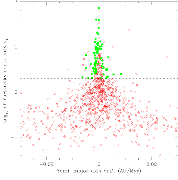
Figure 2: Yarkovsky sensitivity metric $s_{Y}$ plotted as a function of semi-major axis drift rate $da/dt$ for 1,252 numbered NEAs. Data sets with Yarkovsky sensitivity below unity (dashed line) yield unreliable results, including large rates and large error bars. Our selection criteria require $s_{Y}>2$ (dotted line) and SNR $>1$. The 80 objects that meet both selection criteria are shown in green. About 26 of these 80 NEAs are eliminated by the sparse test and orbital coverage requirements (see Section 2.3).

After our process of selection and elimination (Section 2.3), we were left with 54 NEAs that exhibit some of the most reliable and strongest drift rates. Although we report objects with $s_{Y}>2$, we have the most confidence in objects with highest Yarkovsky sensitivity, and we show objects in order of decreasing $s_{Y}$ value in our figures.

We examined the impact of various choices of reject/recover thresholds when rejecting outlier observations (Fig. 3). At moderate values of the rejection threshold (i.e. eliminating less than $\sim$5% of observations), best-fit values are consistent with one another. In this regime, results are fairly robust against the choice of rejection thresholds. However results do become sensitive to rejection thresholds when a larger fraction of observations is rejected. As the reject/recover thresholds become more stringent, astrometry with evidence of semi-major axis drift is preferentially rejected, and the best-fit $da/dt$ values approach zero. Our adopted reject/recover thresholds ($\sqrt{8}$/$\sqrt{7}$) are stringent enough that they eliminate obvious outliers, but not so stringent as to suppress the Yarkovsky signal. In 52 out of 54 cases, repeating the outlier rejection step with the best-fit $da/dt$ value resulted in no appreciable change to the result.

Figure 3: Impact of different choices of reject/recover thresholds for the initial rejection step ($da/dt=0$) on the best-fit $da/dt$ values. Results from optical-only fits are shown with their $1\sigma$ error bars for two representative cases, (2202) Pele and (2063) Bacchus. Best-fit $da/dt$ values are consistent with one another in the left half of the diagram. Values to the right of 2.3/2.2 (Pele) and 2.5/2.4 (Bacchus) have SNR less than unity and would not meet our selection criteria. Our adopted reject/recover thresholds are $\sqrt{8}=2.828$ and $\sqrt{7}=2.646$.

As a validation step, we compared the semi-major axis drift rates obtained with our procedure (both optical-only and radar+optical) to previously published values (Table 2). We found good agreement for Golevka (Chesley et al., 2003, 2008) and 1992 BF (Vokrouhlický et al., 2008), and for most, but not all, NEAs included in a similar study done by Chesley et al. (2008). The differences between our results and those of Chesley et al. (2008) can probably be attributed to our use of debiased data, of improved data weights, and of longer observational arcs extending to 2012. Eight objects included in Table 2 meet our selection criteria for detailed analysis in the rest of this paper: (1620) Geographos, (1685) Toro, (1862) Apollo, (1865) Cerberus, (2063) Bacchus, (2100) Ra-Shalom, (2340) Hathor, and (152563) 1992 BF.

Table 2: Comparison of our optical-only results to radar+optical (r+o) results and to the results of a previous study by Chesley et al. (2008). Best-fit $da/dt$ values in units of 10^-4 AU/Myr and their one-sigma uncertainties are listed for optical-only and radar+optical observations. Also shown is the root-mean-square (RMS) of weighted residuals for the gravity-only ($da/dt=0$) solution and for the non-zero $da/dt$ solution (RMS’). We restrict the radar analysis to those objects that have range measurements on at least two apparitions; this excludes (1685) Toro, (1865) Cerberus, (2063) Bacchus, (2340) Hathor, (85953) 1999 FK21, and (152563) 1992 BF.

NEA	radar	radar	r+o	optical-only	r+o	Chesley 08
	RMS	RMS’	RMS’	$da/dt$	$da/dt$	$da/dt$
(1620) Geographos	0.393	0.356	0.55	$-2.43\pm 0.7$	$-2.52\pm 0.6$	$-1.18\pm 0.39$
(1685) Toro	$\cdots$	$\cdots$	0.51	$-1.40\pm 0.7$	$\cdots$	$-0.52\pm 0.27$
(1862) Apollo	1.111	0.403	0.61	$-1.79\pm 0.6$	$-2.38\pm 0.3$	$-2.44\pm 0.26$
(1865) Cerberus	$\cdots$	$\cdots$	0.54	$-5.11\pm 2.7$	$\cdots$	$-7.80\pm 2.28$
(2063) Bacchus	$\cdots$	$\cdots$	0.59	$-4.17\pm 3.7$	$\cdots$	$-10.59\pm 2.21$
(2100) Ra-Shalom	0.488	0.594	0.51	$-4.79\pm 2.2$	$-5.45\pm 1.5$	$-7.09\pm 0.88$
(2340) Hathor	$\cdots$	$\cdots$	0.67	$-14.55\pm 3.6$	$\cdots$	$-13.94\pm 3.84$
(6489) Golevka	0.879	0.387	0.61	$-2.05\pm 12.6$	$-5.74\pm 0.7$	$-6.39\pm 0.44$
(54509) YORP	0.796	0.260	0.55	$-25.98\pm 37.4$	$-35.63\pm 10.5$	$-25.12\pm 6.18$
(85953) 1999 FK21	$\cdots$	$\cdots$	0.56	$-10.44\pm 1.5$	$\cdots$	$-14.13\pm 2.35$
(101955) 1999 RQ36	15.694	0.127	0.39	$-12.90\pm 7.1$	$-18.9\pm 0.2$	$-15.69\pm 4.99$
(152563) 1992 BF	$\cdots$	$\cdots$	0.60	$-12.84\pm 1.0$	$\cdots$	$-10.78\pm 0.73$

This object is in a Sun-Earth horseshoe orbit (Taylor et al., 2007). This object experiences perihelion precession of $\sim$16 arcseconds/century (Margot & Giorgini, 2010).This object is the target of the OSIRIS-REx mission (Chesley et al., 2012). Fits to this object use the astrometry corrections given in Vokrouhlický et al. (2008) for the 1953 observations, which we did not subject to rejection.

Several conclusions can be drawn from the data presented in Table 2. First, the RMS values indicate excellent fits to the astrometry. Second, the solutions with non-zero $da/dt$ values provide a much better match to the radar data than the gravity-only solutions, with typical RMS values decreasing by a factor of 2 or more. Third, radar+optical estimates have consistently lower error bars than optical-only estimates, sometimes dramatically so, which is typical in NEA studies. Finally, there is a generally good agreement between the optical-only $da/dt$ values and the radar+optical $da/dt$ values, indicating that the optical-only technique is a useful tool that can be used even in the absence of radar data.

Drift rates for the 54 NEAs that pass our selection criteria are presented in Table 3 along with orbital elements and physical properties. If an object has both a optical-only and a radar+optical value, we used the more accurate radar+optical value in the following figures and calculations (unless specified otherwise). We used Equation (2) with a density of 1,200 kg m^-3 to compute efficiency factors $f_{Y}$ and found that objects divided roughly into two groups.

In the first group of 42 objects with $f_{Y}\leq 2\times 10^{-5}$, most observed $da/dt$ values are consistent (within $1\sigma$) with Yarkovsky predictions. We refer to these objects as Yarkovsky-dominated (Figs. 4 and 5). In the second group of 12 objects with $f_{Y}>2\times 10^{-5}$ the observed $da/dt$ values are somewhat larger than Yarkovsky predictions, but improvements in the knowledge of physical properties or in Yarkovsky modeling could plausibly bring some of the observed rates in agreement with predictions. We refer to these objects as possibly Yarkovsky-dominated (Fig. 6).

Figures 4 and 5 indicate that there is generally agreement between observations and numerical estimates of Yarkovsky drift rates for NEAs with $f_{Y}\leq 2\times 10^{-5}$. These data suggest that $f_{Y}\sim 10^{-5}$ represents a typical efficiency for the Yarkovsky process. Predicted values are based on calculations with obliquities of $0^{\circ}$ and $180^{\circ}$, therefore, observed rates that are lower than predictions could still be due to the Yarkovsky effect.

The majority of objects in Fig. 5 appear to exceed predictions. This is a consequence of the SNR $>1$ selection criterion, as it eliminates objects with lower $da/dt$ values.

On the basis of the entire sample of measured drifts for objects with $s_{Y}>2$, we can compute average properties for observed Yarkovsky rates and efficiencies. The mean, mean weighted by uncertainties, median, and dispersion are shown in Table 4. The aggregate properties are comparable if we restrict objects to the subset with SNR $>$ 1, except for slightly increased $da/dt$ rates (median rate of $\sim 12\times 10^{-4}$ AU/Myr instead of $\sim 7\times 10^{-4}$ AU/Myr), as expected. The Yarkovsky process appears to have an efficiency $f_{Y}$ of order $10^{-5}$, with a fairly small dispersion. Because the Yarkovsky efficiency scales with density ($f_{Y}|_{\rho}=f_{Y}|_{1,200}\times{\rho}/{1,200\ \rm{kg\ m}^{-3}}$) some of the observed scatter is due to density variations.

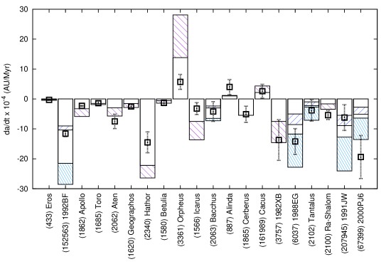
Figure 4: Measured and predicted drift values for 20 asteroids with Yarkovsky-dominated drifts, ordered by decreasing value of Yarkovsky sensitivity. Best fits to optical-only data are shown as squares with dotted $1\sigma$ error bars. Shaded boxes show a range of predicted Yarkovsky rates representing different compositions (Table 1). As predicted Yarkovsky values were calculated assuming $0^{\circ}$ or $180^{\circ}$ obliquity, the shaded boxes represent maximum drifts for the object. Therefore, a fit that lies between a shaded box and $da/dt=0$ is considered to have good agreement. Objects with a single corresponding shaded box have a known diameter (Table 3). Objects with two shaded boxes did not have known diameters, and were modeled using diameters derived from assumed albedos (45% in light blue, larger predicted drift magnitudes, and 5% in dark blue, smaller predicted drift magnitudes). The vertical extents of the shaded boxes represent the range of compositional types described in Table 1, with the larger absolute values representing the “rubble pile” composition, and the lower absolute values representing the “rock chunk” composition.

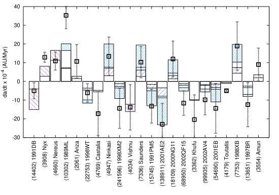
Figure 5: Measured and predicted drift values for an additional 22 asteroids with Yarkovsky-dominated drifts, ordered by decreasing value of Yarkovsky sensitivity. Symbols are as in Fig. 4. The observed rates for the majority of objects shown in this figure appear to exceed predicted values. This is a consequence of the SNR $>1$ selection criterion which eliminates objects with lower $da/dt$ values.

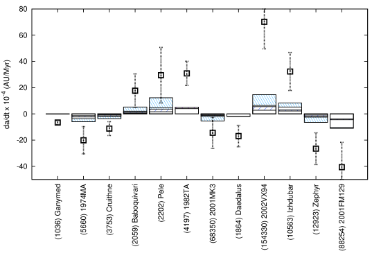
Figure 6: Measured and predicted drift values for 12 asteroids with possible Yarkovsky-dominated drifts, defined as objects with Yarkovsky efficiency $f_{Y}$ exceeding 2 $\times 10^{-5}$. Symbols are as in Fig. 4. Most objects in this figure have measured drifts that lie outside of the range of values expected on the basis of Yarkovsky models. This could be due to inaccuracies in our knowledge of physical properties, faulty astrometry, or modeling errors.

4 Discussion

In this section we examine several consequences of our results. First we discuss how the Yarkovsky drifts can inform us about asteroid physical properties, spin states, and trajectories. Then we discuss binary asteroid (1862) Apollo and the curious case of asteroid (1036) Ganymed. Finally we discuss the possible mechanisms for non-Yarkovsky driven rates, including association with meteoroid streams and rock comet phenomenon.

4.1 Yarkovsky-derived constraints on asteroid physical properties

Because a clear connection exists between asteroid physical properties and Yarkovsky drifts, we explored the constraints that can be placed on bulk density and surface thermal conductivity for seven objects with well-known diameters and (excepting one case) spin periods: (1620) Geographos, (1862) Apollo, (2100) Ra-Shalom, (2062) Aten, (2340) Hathor, (1566) Icarus, and (3361) Orpheus. We compared the measured Yarkovsky rates to numerical estimates obtained with a range of physical parameters. For these estimates, we assumed a constant heat capacity $C=500$ J kg^-1 K^-1 (Table 1) and a single value of the bulk density of the surface $\rho_{s}=1,700$ kg m^-3, but we explore a wide range of bulk density and surface thermal conductivity values. Because the obliquities are uncertain or ambiguous in many cases, we chose to illustrate outcomes for two obliquity values, typically 180^∘ and 135^∘.

Our results are shown in Figures 7 and 8, which are similar to Fig. 4 in Chesley et al. (2003). The shaded range consistent with the $1\sigma$ confidence limits on $da/dt$ delineates the space of acceptable bulk densities and thermal conductivities, assuming that the Yarkovsky effect is being modeled correctly. By acceptable, we mean consistent with observed $da/dt$ values, even though some of the $K-\rho$ values may not be appropriate for asteroids.

Infrared observations indicate that (2100) Ra-Shalom has a thermal conductivity between 0.1 and 1 W m^-1 K^-1 (Delbó et al., 2003; Shepard et al., 2008). If we assume a minimum bulk density of 1,500 kg m^-3, this conductivity value is consistent with the range suggested by our Yarkovsky rate determination.

If we make the same minimum density assumption for (1620) Geographos, our measurements suggest that its surface thermal conductivity is greater than 0.002 W m^-1 K^-1.

For (1862) Apollo, we show the range of physical properties that are consistent with both the optical-only fits and the radar+optical fits. The precision of the radar measurements dramatically shrinks the size of the measured error bars, with correspondingly tighter constraints on density and surface thermal conductivity. This example illustrates that reliable obliquity determinations will be important to extract physical properties from Yarkovsky rate determinations.

Our measurement of (2062) Aten’s drift provides some useful insights. If we assume that its bulk density exceeds $1,500$ kg m^-3, then its surface thermal conductivity $K$ must exceed 0.3 W m^-1 K^-1. Furthermore, if we assume that its bulk density exceeds $1,600$ kg m^-3, the $1\sigma$ confidence region on the measured Yarkovsky drift suggests that its obliquity is between $180^{\circ}-135^{\circ}$.

The Yarkovsky simulations for (2340) Hathor were computed with an assumed spin period of 4.5 hours. If the actual period is longer, the curves shown would shift to the left, and if the period is shorter, the curves would shift to the right. Consequently, we cannot make inferences about the $K$ value for this object until its spin period is measured. However, looking at the height of the curve, and with an assumption that the object’s bulk density is greater than $1,500$ kg m^-3, we can conclude that (2340) Hathor likely has an obliquity lower than $180^{\circ}$.

The assumption of $135^{\circ}$ or $180^{\circ}$ obliquity for (1566) Icarus restricts this object to low surface conductivity values and low bulk density values, or high surface conductivity values and high bulk density values. Although these obliquities do produce physically plausible parameter combinations, it seems likely that the obliquity for this object is $\leq 135^{\circ}$.

The curves for (3361) Orpheus were calculated with an assumed geometric albedo of 0.15. As (3361) Orpheus has a positive $da/dt$ value, obliquities were assumed to be $0^{\circ}$ and $45^{\circ}$. The curve representing an obliquity equal to $0^{\circ}$ for this object requires very low ($<0.002$ W m^-1 K^-1) or very high ($>0.7$ W m^-1 K^-1) surface thermal conductivity values for most densities. A more likely scenario is that this object has an obliquity $>0^{\circ}$, or perhaps even $>45^{\circ}$. An independent measurement of the obliquity could be used to validate obliquity constraints derived from Yarkovsky measurements.

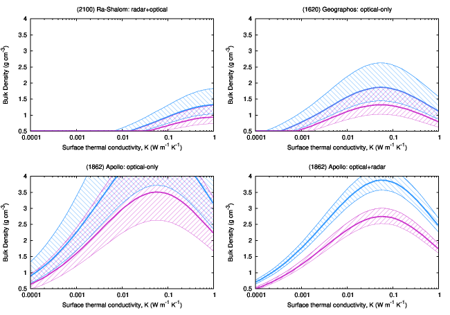
Figure 7: Range of bulk densities and thermal conductivities of three Yarkovsky-dominated asteroids consistent with their observed $da/dt$ values. Blue (top) solid line corresponds to values consistent with best-fit $da/dt$ and $180^{\circ}$ obliquity, pink (lower) solid line corresponds to values consistent with best-fit $da/dt$ and $135^{\circ}$ obliquity. Dashed regions surrounding each solid line encompass the $1\sigma$ confidence limits on the corresponding $da/dt$ determinations. Not all values displayed in this K-$\rho$ space are necessarily appropriate for asteroids. Infrared observations suggest that (2100) Ra-Shalom has a thermal conductivity between 0.1 and 1 W m^-1 K^-1 (Delbó et al., 2003; Shepard et al., 2008), consistent with the range suggested by our Yarkovsky rate determination. For Apollo, we show results for both optical-only and radar+optical determinations. The inclusion of radar data greatly reduces the error bars on the measured drift, and therefore the area of the shaded curves.

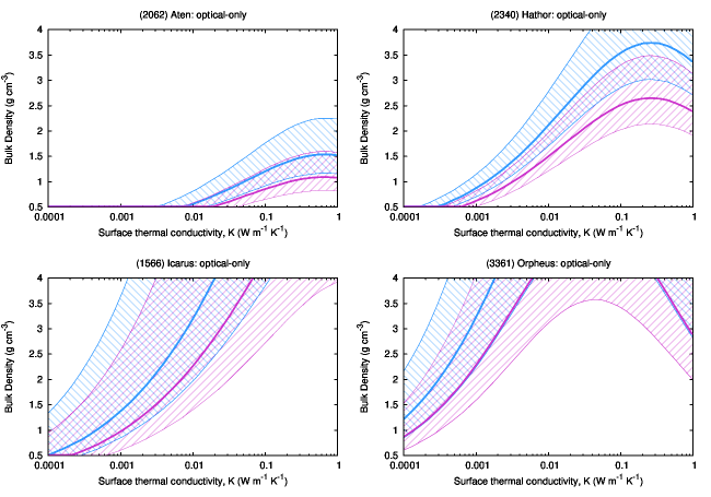
Figure 8: Companion to Fig. 7. Range of bulk densities and thermal conductivities of three Yarkovsky-dominated asteroids consistent with their observed $da/dt$ values. For (2062) Aten and (2340) Hathor, blue (top) solid line corresponds to values consistent with best-fit $da/dt$ and $180^{\circ}$ obliquity, pink (lower) solid line corresponds to values consistent with best-fit $da/dt$ and $135^{\circ}$ obliquity. The constraints for (1566) Icarus suggest that it may have a lower obliquity than those assumed. (3361) Orpheus has a positive drift, so the blue (top) solid line corresponds to values consistent with best-fit $da/dt$ and $0^{\circ}$ obliquity, pink (lower) solid line corresponds to values consistent with best-fit $da/dt$ and $45^{\circ}$ obliquity. Dashed regions surrounding each solid line encompass the $1\sigma$ confidence limits on the corresponding $da/dt$ determinations. Not all values displayed in this K-$\rho$ space are necessarily appropriate for asteroids. A period of 4.5 hours was assumed for (2340) Hathor, and a 0.15 geometric albedo was assumed for (3361) Orpheus.

4.2 Yarkovsky rates and distribution of spin states

La Spina et al. (2004) and Chesley et al. (2008) examined the predominance of retrograde spins and negative Yarkovsky drift rates and concluded that they were consistent with the presumed delivery method of NEAs from the main belt of asteroids. The $\nu_{6}$ and 3:1 resonance regions deliver NEAs to near-Earth space (Bottke et al., 2002a). A main belt asteroid can arrive at the 3:1 resonance at 2.5 AU via a positive (if it originates in the inner main belt) or negative (if it originates in the outer main belt) Yarkovsky drift. However, a main belt asteroid can only arrive at the $\nu_{6}$ resonance (at the inner edge of the main belt) by way of a negative drift. According to Bottke et al. (2002a) and Morbidelli & Vokrouhlický (2003), $30\%-37\%$ of NEAs are transported via the $\nu_{6}$ resonance, with the rest from other resonances. The net result is a preference for retrograde spins.

An observational consequence of this process would be an excess of retrograde rotators in the near-Earth asteroid population. La Spina et al. (2004) conducted a survey of 21 NEAs and found the ratio of retrograde/prograde rotators to be $2.0^{+1}_{-0.7}$.

We note that out of the 42 Yarkovsky-dominated NEAs, 12 have a positive $da/dt$ value. For this sample, our ratio of retrograde/prograde rotators is $2.5\pm 0.1$, similar to the value found by La Spina et al. (2004).

4.3 Impact of drift rates on asteroid trajectory predictions

The semi-major axis drifts described in this paper affect NEA trajectory predictions. An order of magnitude estimate for the along track displacement due to a non-zero $da/dt$ is given in Vokrouhlický et al. (2000):

$$\Delta\rho\simeq 7\dot{a}_{4}(\Delta_{10}t)^{2}a_{AU}^{-3/2}$$ (6)

where $\Delta\rho$ is in units of km, $\dot{a}_{4}$ is $da/dt$ in $10^{-4}$ AU/Myr, $\Delta_{10}t$ is the time difference between observations in tens of years, and $a_{AU}$ is the semimajor axis of the object in AU. For instance, the estimated along-track displacement due to the observed $da/dt$ for (1862) Apollo is 9 km after 10 years. Similarly, the estimated along-track displacement for faster-moving (1864) Daedalus is 67 km after 10 years.

Our data indicate that (101955) 1999 RQ36, the target of the OSIRIS-REx mission, has a measurable Yarkovsky drift of $(-18.9\pm 0.2)\times 10^{-4}$ AU/Myr. Although it has a relatively short arc (12 years) it has been observed three times by radar, allowing for an accurate $da/dt$ measurement. We estimated the along-track displacement of (101955) 1999 RQ36 over the 6-month duration of the OSIRIS-REx mission to be $0.3$ km, which will be easily detectable by a radio science instrument.

4.4 Binary asteroid (1862) Apollo

(1862) Apollo is a binary asteroid (Ostro et al., 2005). Binary asteroids present a unique opportunity for the determination of physical parameters. If mass and density can be measured from the binary orbit and component sizes, the Yarkovsky constraint on thermal conductivity can become much more meaningful. If the orientation of the plane of the mutual orbital can be measured, a plausible obliquity can be assumed, which makes the constraints on thermal properties tighter still. In some cases, actual obliquity measurements can be obtained from shape modeling efforts.

Yeomans (1991, 1992) identified a non-gravitational perturbation acting on the orbit of (1862) Apollo, but was not able to determine a drift magnitude. To $1\sigma$ our observed $da/dt$ value for (1862) Apollo agrees with our Yarkovsky predictions.

4.5 The curious case of (1036) Ganymed

(1036) Ganymed has by far the largest Yarkovsky efficiency value ($f_{Y}\sim 15\times 10^{-5}$) among the objects presented in Table 3. With a nominal value of $\sim-7\times 10^{-4}$ AU/Myr, the measured $da/dt$ value is comparable to that of other NEAs. Combined with Ganymed’s large diameter estimate ($\sim 32$ km based on IRAF measurements), this Yarkovsky rate results in an unusually high $f_{Y}$ value.

How can this anomaly be explained? One possibility is that some of the early astrometry, dating back to 1924, is erroneous. This could be due to measurement errors, timing errors, bias errors, or reference frame conversion errors. We evaluated the semi-major axis drift with various subsets of the available astrometry and found values ranging between $-3\times 10^{-4}$ and $-8\times 10^{-4}$ AU/Myr. On that basis we modified the adopted uncertainties for this object, and our preferred value is $(-6.62_{-1.4}^{+3.6})\times 10^{-4}$ AU/Myr. Doing so does not eliminate the possibility of systematic bias in the astrometry, and we are still left with anomalously high $f_{Y}$ values.

Another possibility is that the diameter of Ganymed, an S-type asteroid, is much smaller than reported. This seems unlikely considering the more recent WISE albedo measurement of $p_{V}=0.212$ (Masiero et al., 2012) which suggests a diameter of $\sim 36$ km.

If Ganymed’s bulk density was especially low, a higher than usual $f_{Y}$ value would be expected, but this would likely explain a factor of 2 or 3 at most, and would not explain the anomalous value.

Perhaps Ganymed departs significantly from a spherical shape, with an effective diameter and mass that are much smaller than those implied by the diameter values reported in the literature. The relatively low lightcurve amplitudes do not seem to support such an argument, unless the asteroid is particularly oblate. In that case one could plausibly arrive at volume and mass estimates that are off by a factor of 5-10.

If we can rule out these possibilities (i.e. Ganymed is roughly spherical with no substantial concavities, its diameter estimate is reasonably accurate, and the early astrometry can be trusted), and if no other modeling error can be identified, then we would be compelled to accept an anomalously high Yarkovsky efficiency for this object.

4.6 Non-Yarkovsky processes

In the course of our study we observed drift values that cannot be accounted for easily by Yarkovsky drift, because they considerably exceed the predicted Yarkovsky rates. In most cases, these can be attributed to poor sensitivity to Yarkovsky influences (Fig. 2). Therefore, the high rates can generally be safely discarded. In other cases, the high rates may be due to erroneous optical astrometry or mismodeling of asteroid-asteroid perturbations. However we cannot entirely rule out the possibility that some of the high drift rates are secure and will be confirmed by further observation and analysis. If the high rates cannot be ascribed to poor Yarkovsky sensitivity or faulty astrometry, one would need to invoke other non-gravitational forces.

One possibility is that orbits are perturbed when NEAs are losing gas or dust in an anisotropic manner. To estimate a rough rate of mass loss that would be needed to account for the drifts measured, we used the basic thrust equation

$$F=qV_{e}$$ (7)

where $F$ is the force, $q$ is the rate at which the mass departs the asteroid, and $V_{e}$ is the ejection speed. For an asteroid of mass $m$ this yields

$$a_{\rm mass\ loss}=\frac{qV_{e}}{m}$$ (8)

which can be incorporated into Gauss’ form of Lagrange’s planetary equations (Danby, 1992) as an acceleration aligned with the velocity of the object. The dependence of the force on heliocentric distance $r$ is not known precisely; we assumed $F\propto r^{-2}$, similar to the Yarkovsky dependence, for simplicity, and because the amount of outgassing likely scales with the amount of incident radiation (as in Fig. 4 of Delsemme (1982)). We assumed $V_{e}=1.5$ m s^-1, the value derived by Hsieh et al. (2004) for 133P/Elst-Pizarro, and we assumed that the mass is departing in the optimal thrust direction.

We quantified the mass loss rates needed to produce the observed drifts of NEAs with the highest Yarkovsky efficiencies. We estimated a rate of 0.16 kg s^-1 for (154330) 2002 VX94 and 2.3 kg s^-1 for (7889) 1994 LX. Although these estimates represent the minimum amount of mass loss necessary to account for the observed drifts (if due to mass loss), they are smaller than typical levels from comets. Comets have mass loss rates that span a wide range of values. On the high side a rate of $2\times 10^{6}$ kg s^-1 was estimated for Hale-Bopp (Jewitt & Matthews, 1999). On the low side Ishiguro et al. (2007) measured mass loss rates for three comets, averaged over their orbits: 2P/Encke ($48\pm 20$ kg s^-1), 22P/Kopff ($17\pm 3$ kg s^-1), and 65P/Gunn ($27\pm 9$ kg s^-1). Mass loss rates of active asteroids have been estimated to be in the range from $\leq 0.04$ kg s^-1 (113P/Elst-Pizarro) to $\leq 150$ kg s^-1 (107P/Wilson-Harrington) (Jewitt, 2012).

Mass loss does not seem to be a viable mechanism to explain the semi-major axis drift rate of (1036) Ganymed, as it would require a minimum mass loss rate of $\sim$2,500 kg s^-1. This would presumably have left detectable observational signatures, which have not been reported to date.

We explore a couple of possibilities for mass loss mechanisms that could cause semi-major axis drifts.

4.6.1 Associations with meteoroid streams

To our knowledge, (433) Eros, (1566) Icarus, (1620) Geographos, (1685) Toro, (1862) Apollo, and 1982 TA are the only objects in our sample to have been associated with a meteoroid stream. Sekanina (1976) found a weak correlation between the first five objects and various streams using the “dissimilarity criterion”. However, this metric was later described as not convincing by Jenniskens (2008), and current literature does not support such associations. In our results, Apollo shows good agreement with Yarkovsky predictions, with $f_{Y}=0.25\times 10^{-5}$. The Yarkovsky force is therefore a plausible cause of Apollo’s observed semi-major axis drift.

4.6.2 Rock comet phenomenon

The brightening of (3200) Phaethon, the parent body of the Geminid meteor shower, has been attributed to a “rock comet” phenomenon (Jewitt & Li, 2010). With a perihelion at 0.14 AU, (3200) Phaethon’s surface temperatures have been estimated by Jewitt & Li (2010) to be in the range $746<T<1050$ K. The authors propose that these high surface temperatures could create thermal gradients in the body, resulting in thermal fracturing that would release dust. The resulting mass loss would affect the orbit. The combination of mass loss due to decomposing hydrated minerals and thermal fracturing led the authors to term (3200) Phaethon a “rock comet”. A moderate amount ($\sim$ 1 kg s^-1) of mass lost in an anisotropic manner by “rock comets” could explain the observed semi-major axis drift rates.

5 Conclusions

Modeling of the Yarkovsky effect is needed to improve trajectory predictions of near-Earth asteroids and to refine our understanding of the dynamics of small bodies. Using fits to astrometric data, we identified semi-major axis drifts in 54 NEAs, 42 of which show good agreement with numerical estimates of Yarkovsky drifts, indicating that they are likely Yarkovsky-dominated. These objects exhibit Yarkovsky efficiencies of $\sim$10^-5, where the efficiency describes the ratio of the change in orbital energy to incident solar radiation energy. 12 objects in our sample have drifts that exceed nominal Yarkovsky predictions and are labeled possibly Yarkovsky-dominated. Improvements in the knowledge of physical properties or in thermal modeling could bring these drift rates in better agreement with results from numerical models. However, if the high rates are confirmed by additional observations and analysis, they would be indicative of the presence of other non-gravitational forces, such as that resulting from a loss of mass.

Table 3: Semi-major Axis Drift Rates

NEA		$a$	$e$	$i$	$D$	$P$	$p_{V}$	Arc	$(da/dt)_{\rm o}$	$1\sigma$	$(da/dt)_{\rm r+o}$	$1\sigma$	SNR	$s_{Y}$	$f_{Y}$
		(AU)		(deg)	(km)	(h)			(10-4 AU/Myr)		(10-4 AU/Myr)				$\times 10^{-5}$
(433)	Eros	1.46	0.22	10.83	16.84	5.270	0.25	1893-2012	-0.3	0.2	$\cdots$	$\cdots$	1.81	70.56	0.38
(152563)	1992 BF	0.91	0.27	7.25	0.42$\dagger$	$\cdots$	$\cdots$	1992-2011	-11.6	1.0	$\cdots$	$\cdots$	11.26	40.28	0.37
(1862)	Apollo	1.47	0.56	6.35	1.50	3.065	0.25	1957-2012	-1.8	0.6	-2.3	0.2	11.50	36.11	0.23
(1685)	Toro	1.37	0.44	9.38	3.40	10.1995	0.31	1948-2010	-1.4	0.7	$\cdots$	$\cdots$	2.00	24.06	0.34
(2062)	Aten	0.97	0.18	18.93	1.10	40.77	0.26	1955-2012	-7.5	2.4	$\cdots$	$\cdots$	3.17	19.94	0.65
(1620)	Geographos	1.25	0.34	13.34	2.56	5.22204	0.3258	1951-2012	-2.4	0.7	-2.5	0.6	3.85	18.15	0.48
(2340)	Hathor	0.84	0.45	5.85	0.30	$\cdots$	$\cdots$	1976-2012	-14.5	3.5	$\cdots$	$\cdots$	4.11	15.32	0.31
(1580)	Betulia	2.20	0.49	52.11	5.80	6.1324	0.08	1950-2010	-1.4	2.0	-1.3	0.9	1.46	13.45	0.53
(3361)	Orpheus	1.21	0.32	2.69	0.30	3.58	$\cdots$	1982-2009	5.7	2.5	$\cdots$	$\cdots$	2.25	13.04	0.13
(1566)	Icarus	1.08	0.83	22.83	1.00	2.273	0.51	1949-2009	-3.2	2.0	$\cdots$	$\cdots$	1.62	11.86	0.14
(2063)	Bacchus	1.08	0.35	9.43	1.35$\dagger$	14.90	$\cdots$	1977-2007	-4.2	3.3	$\cdots$	$\cdots$	1.26	10.58	0.42
(887)	Alinda	2.48	0.57	9.36	4.20	73.97	0.31	1918-2008	4.0	2.5	$\cdots$	$\cdots$	1.59	9.42	1.12
(1865)	Cerberus	1.08	0.47	16.10	1.20	6.810	0.22	1971-2008	-5.1	2.7	$\cdots$	$\cdots$	1.90	9.20	0.44
(161989)	Cacus	1.12	0.21	26.06	1.90	3.7538	0.09	1978-2010	2.6	2.3	$\cdots$	$\cdots$	1.12	8.94	0.39
(3757)	1982 XB	1.83	0.45	3.87	0.50	9.0046	0.18	1982-2008	-13.7	6.8	$\cdots$	$\cdots$	2.04	8.82	0.49
(6037)	1988 EG	1.27	0.50	3.50	0.65$\dagger$	2.760	$\cdots$	1988-2007	-14.2	4.3	$\cdots$	$\cdots$	3.34	8.51	0.64
(2102)	Tantalus	1.29	0.30	64.01	2.04$\dagger$	2.391	$\cdots$	1975-2008	-3.8	3.6	$\cdots$	$\cdots$	1.08	8.31	0.60
(2100)	Ra-Shalom	0.83	0.44	15.76	2.30	19.797	0.13	1975-2009	-4.8	2.2	-5.4	1.5	3.67	8.30	0.90
(207945)	1991 JW	1.04	0.12	8.71	0.52$\dagger$	$\cdots$	$\cdots$	1955-2009	-6.2	4.3	$\cdots$	$\cdots$	1.42	8.00	0.26
(67399)	2000 PJ6	1.30	0.35	14.69	0.96$\dagger$	$\cdots$	$\cdots$	1951-2009	-19.4	7.2	$\cdots$	$\cdots$	2.71	7.34	1.40
(1036)	Ganymed	2.66	0.53	26.70	31.66	10.31	0.2926	1924-2012	-6.6	1.5	$\cdots$	$\cdots$	4.41	7.28	14.23
(14402)	1991 DB	1.72	0.40	11.42	0.60	2.266	0.14	1991-2009	-5.0	4.3	$\cdots$	$\cdots$	1.19	7.05	0.22
(3908)	Nyx	1.93	0.46	2.18	1.00	4.42601	0.23	1980-2009	9.8	3.2	12.9	2.7	4.71	5.52	0.92
(4660)	Nereus	1.49	0.36	1.43	0.33	15.1	0.55	1981-2010	7.3	5.6	10.9	4.8	2.29	5.46	0.27
(5660)	1974 MA	1.79	0.76	38.06	2.57$\dagger$	17.5	$\cdots$	1974-2005	-20.1	10.4	$\cdots$	$\cdots$	1.92	5.46	2.68
(10302)	1989 ML	1.27	0.14	4.38	0.45$\dagger$	19.	$\cdots$	1989-2006	35.3	7.1	$\cdots$	$\cdots$	4.96	5.33	1.26
(2061)	Anza	2.26	0.54	3.77	2.60	11.50	$\cdots$	1960-2012	10.7	9.0	$\cdots$	$\cdots$	1.19	5.00	1.88
(22753)	1998 WT	1.22	0.57	3.20	1.02$\dagger$	10.24	$\cdots$	1955-2009	-5.4	5.0	-6.1	4.9	1.26	4.95	0.41
(3753)	Cruithne	1.00	0.51	19.81	3.39$\dagger$	27.4	$\cdots$	1973-2010	-11.2	5.3	$\cdots$	$\cdots$	2.12	4.84	2.61
(4769)	Castalia	1.06	0.48	8.89	1.40	4.095	$\cdots$	1989-2011	-17.2	11.7	$\cdots$	$\cdots$	1.47	4.59	1.69
(4947)	Ninkasi	1.37	0.17	15.65	0.65$\dagger$	$\cdots$	$\cdots$	1978-2009	13.4	10.3	$\cdots$	$\cdots$	1.30	4.23	0.69
(241596)	1998 XM2	1.80	0.34	27.10	1.41$\dagger$	$\cdots$	$\cdots$	1952-2011	-14.4	10.7	$\cdots$	$\cdots$	1.35	4.23	1.53
(4034)	Vishnu	1.06	0.44	11.17	0.42	$\cdots$	0.52	1986-2009	-13.8	12.1	$\cdots$	$\cdots$	1.14	3.72	0.42
(7336)	Saunders	2.31	0.48	7.17	0.65$\dagger$	6.423	$\cdots$	1982-2010	10.3	8.3	$\cdots$	$\cdots$	1.25	3.50	0.47
(2059)	Baboquivari	2.64	0.53	11.04	2.46$\dagger$	$\cdots$	$\cdots$	1963-2009	17.7	12.8	$\cdots$	$\cdots$	1.38	3.42	2.96
(15745)	1991 PM5	1.72	0.25	14.42	0.98$\dagger$	$\cdots$	$\cdots$	1982-2007	-13.2	9.0	$\cdots$	$\cdots$	1.46	3.39	1.00
(138911)	2001 AE2	1.35	0.08	1.66	0.56$\dagger$	$\cdots$	$\cdots$	1984-2012	-22.9	11.2	$\cdots$	$\cdots$	2.04	3.38	1.02
(18109)	2000 NG11	1.88	0.37	0.81	1.12$\dagger$	4.2534	$\cdots$	1951-2005	12.0	9.6	$\cdots$	$\cdots$	1.25	3.21	1.00
(2202)	Pele	2.29	0.51	8.74	1.07$\dagger$	$\cdots$	$\cdots$	1972-2008	29.5	21.2	$\cdots$	$\cdots$	1.39	2.98	2.18
(68950)	2002 QF15	1.06	0.34	25.16	2.03$\dagger$	29.	$\cdots$	1955-2008	-11.6	6.5	$\cdots$	$\cdots$	1.80	2.96	1.78
(4197)	1982 TA	2.30	0.77	12.57	1.80	3.5380	0.37	1954-2010	30.9	9.2	$\cdots$	$\cdots$	3.36	2.88	2.84
(3362)	Khufu	0.99	0.47	9.92	0.70	$\cdots$	0.21	1984-2004	-20.4	13.2	$\cdots$	$\cdots$	1.54	2.87	1.01
(99935)	2002 AV4	1.65	0.64	12.76	2.46$\dagger$	$\cdots$	$\cdots$	1955-2011	-9.8	8.0	$\cdots$	$\cdots$	1.23	2.73	1.48
(68350)	2001 MK3	1.67	0.25	29.56	2.43$\dagger$	3.24	$\cdots$	1955-2007	-14.4	11.9	$\cdots$	$\cdots$	1.21	2.61	2.73
(54690)	2001 EB	1.63	0.26	35.36	1.18$\dagger$	$\cdots$	$\cdots$	1952-2009	-14.4	13.3	$\cdots$	$\cdots$	1.08	2.56	1.31
(4179)	Toutatis	2.53	0.63	0.45	5.40	176.	$\cdots$	1976-2011	-18.4	4.3	-5.0	0.6	8.33	2.44	1.68
(1864)	Daedalus	1.46	0.61	22.20	3.70	8.572	$\cdots$	1971-2006	-16.9	8.2	$\cdots$	$\cdots$	2.06	2.44	3.97
(154330)	2002 VX94	1.48	0.41	7.16	0.90$\dagger$	$\cdots$	$\cdots$	1986-2011	70.2	20.6	$\cdots$	$\cdots$	3.42	2.41	4.64
(7753)	1988 XB	1.47	0.48	3.12	0.68$\dagger$	$\cdots$	$\cdots$	1988-2012	18.9	12.9	$\cdots$	$\cdots$	1.46	2.39	0.90
(10563)	Izhdubar	1.01	0.27	63.46	1.48$\dagger$	$\cdots$	$\cdots$	1991-2010	32.3	14.5	$\cdots$	$\cdots$	2.23	2.19	3.70
(13651)	1997 BR	1.34	0.31	17.25	1.07$\dagger$	33.644	$\cdots$	1980-2011	-12.4	11.8	$\cdots$	$\cdots$	1.06	2.18	1.02
(12923)	Zephyr	1.96	0.49	5.29	2.14$\dagger$	3.891	$\cdots$	1955-2012	-26.5	12.1	$\cdots$	$\cdots$	2.19	2.05	3.97
(3554)	Amun	0.97	0.28	23.36	2.48	2.530	0.1284	1986-2012	9.0	8.8	$\cdots$	$\cdots$	1.03	2.05	1.73
(88254)	2001 FM129	1.18	0.63	1.52	1.19$\dagger$	$\cdots$	$\cdots$	1978-2008	-40.6	18.9	$\cdots$	$\cdots$	2.15	2.05	3.01

Table 4: Statistical properties of observed Yarkovsky rates and efficiencies.

	abs$(da/dt)\times 10^{-4}$ AU/Myr
Yarkovsky rate	mean	weighted mean	median	stdev
objects with $f_{Y}<2\times 10^{-5}$	7.6	4.4	5.6	6.4
objects with $f_{Y}>2\times 10^{-5}$	27.0	18.5	20.1	18.7
all objects	10.4	5.2	7.3	11.4
	$f_{Y}\times 10^{-5}$
Yarkovsky efficiency	mean	weighted mean	median	stdev
objects with $f_{Y}<2\times 10^{-5}$	0.67	0.53	0.50	0.51
objects with $f_{Y}>2\times 10^{-5}$	4.50	7.47	3.01	3.38
all objects	1.22	0.89	0.65	1.91

References

- Bottke et al. (2002a) Bottke, W. F., Morbidelli, A., Jedicke, R., Petit, J., Levison, H. F., Michel, P., & Metcalfe, T. S. 2002a, Icarus, 156, 399
- Bottke et al. (2002b) Bottke, Jr., W. F., Vokrouhlický, D., Rubincam, D. P., & Brož, M. 2002b, Asteroids III, 395
- Bottke et al. (2006) Bottke, Jr., W. F., Vokrouhlický, D., Rubincam, D. P., & Nesvorný, D. 2006, Annual Review of Earth and Planetary Sciences, 34, 157
- Bowell et al. (1989) Bowell, E., Hapke, B., Domingue, D., Lumme, K., Peltoniemi, J., & Harris, A. W. 1989, in Asteroids II, 524–556
- Chamberlin (2008) Chamberlin, A. B. 2008, Bulletin of the American Astronomical Society, 40
- Chesley et al. (2003) Chesley, S., Ostro, S., Vokrouhlický, D., Čapek, D., Giorgini, J., Nolan, M., Margot, J. L., Hine, A., Benner, L., & Chamberlin, A. 2003, Science, 302, 1739
- Chesley (2006) Chesley, S. R. 2006, Asteroids, Comets, and Meteors conference abstracts
- Chesley et al. (2010) Chesley, S. R., Baer, J., & Monet, D. G. 2010, Icarus, 210, 158
- Chesley et al. (2008) Chesley, S. R., Vokrouhlický, D., Ostro, S. J., Benner, L. A. M., Margot, J. L., Matson, R. L., Nolan, M. C., & Shepard, M. K. 2008, LPI Contributions, 1405, 8330
- Chesley et al. (2012) Chesley, S. R. et al. 2012, Asteroids, Comets, Meteors conference abstracts
- Danby (1992) Danby, J. M. A. 1992, Fundamentals of Celestial Mechanics (Willmann-Bell, Inc)
- Delbó et al. (2007) Delbó, M., dell’Oro, A., Harris, A. W., Mottola, S., & Mueller, M. 2007, Icarus, 190, 236
- Delbó et al. (2003) Delbó, M., Harris, A. W., Binzel, R. P., Pravec, P., & Davies, J. K. 2003, Icarus, 166, 116
- Delsemme (1982) Delsemme, A. H. 1982, in Comets, ed. L. L. Wilkening, 85–130
- Giorgini et al. (2008) Giorgini, J. D., Benner, L. A. M., Ostro, S. J., Nolan, M. C., & Busch, M. W. 2008, Icarus, 193, 1
- Giorgini et al. (2002) Giorgini, J. D., Ostro, S. J., Benner, L. A. M., Chodas, P. W., Chesley, S. R., Hudson, R. S., Nolan, M. C., Klemola, A. R., Standish, E. M., Jurgens, R. F., Rose, R., Chamberlin, A. B., Yeomans, D. K., & Margot, J. L. 2002, Science, 296, 132
- Goldreich & Sari (2009) Goldreich, P. & Sari, R. 2009, The Astrophysical Journal, 691, 54
- Hsieh et al. (2004) Hsieh, H. H., Jewitt, D. C., & Fernández, Y. R. 2004, The Astronomical Journal, 127, 2997
- Hütter & Kömle (2008) Hütter, E. S. & Kömle, N. I. 2008, in 5th European Thermal-Sciences Conference, The Netherlands
- Ishiguro et al. (2007) Ishiguro, M., Sarugaku, Y., Ueno, M., Miura, N., Usui, F., Chun, M.-Y., & Kwon, S. M. 2007, Icarus, 189, 169
- Jenniskens (2008) Jenniskens, P. 2008, Earth Moon and Planets, 102, 505
- Jewitt (2012) Jewitt, D. 2012, The Astronomical Journal, 143, 66
- Jewitt & Li (2010) Jewitt, D. & Li, J. 2010, The Astronomical Journal, 140, 1519
- Jewitt & Matthews (1999) Jewitt, D. & Matthews, H. 1999, The Astronomical Journal, 117, 1056
- Konopliv et al. (2011) Konopliv, A. S., Asmar, S. W., Folkner, W. M., Karatekin, Ö., Nunes, D. C., Smrekar, S. E., Yoder, C. F., & Zuber, M. T. 2011, Icarus, 211, 401
- La Spina et al. (2004) La Spina, A., Paolicchi, P., Kryszczynska, A., & Pravec, P. 2004, Nature, 428, 400
- Margot & Giorgini (2010) Margot, J. L. & Giorgini, J. D. 2010, in IAU Symposium, ed. S. A. Klioner, P. K. Seidelmann, & M. H. Soffel, Vol. 261, 183–188
- Masiero et al. (2012) Masiero, J. R., Mainzer, A. K., Grav, T., Bauer, J. M., Wright, E. L., McMillan, R. S., Tholen, D. J., & Blain, A. W. 2012, The Astrophysical Journal, 749, 104
- Milani et al. (2009) Milani, A., Chesley, S. R., Sansaturio, M. E., Bernardi, F., Valsecchi, G. B., & Arratia, O. 2009, Icarus, 203, 460
- Milani & Gronchi (2009) Milani, A. & Gronchi, G. 2009, Theory of Orbit Determination (Cambridge University Press)
- Morbidelli & Vokrouhlický (2003) Morbidelli, A. & Vokrouhlický, D. 2003, Icarus, 163, 120
- Opeil et al. (2010) Opeil, C., Consolmagno, G., & Britt, D. 2010, Icarus, 208, 449
- Ostro et al. (2005) Ostro, S. J., Benner, L. A. M., Giorgini, J. D., Nolan, M. C., Hine, A. A., Howell, E. S., Margot, J. L., Magri, C., & Shepard, M. K. 2005, IAU Circular, 8627
- Pravec & Harris (2000) Pravec, P. & Harris, A. 2000, Icarus, 148, 12
- Pravec & Harris (2007) Pravec, P. & Harris, A. W. 2007, Icarus, 190, 250
- Press et al. (1992) Press, W. H., Teukolsky, S. A., Vetterling, W. T., & Flannery, B. P. 1992, Numerical Recipes in C (2nd ed.): The Art of Scientific Computing (New York, NY, USA: Cambridge University Press)
- Sekanina (1976) Sekanina, Z. 1976, Icarus, 27, 265
- Shepard et al. (2008) Shepard, M. K., Clark, B. E., Nolan, M. C., Benner, L. A. M., Ostro, S. J., Giorgini, J. D., Vilas, F., Jarvis, K., Lederer, S., Lim, L. F., McConnochie, T., Bell, J., Margot, J. L., Rivkin, A., Magri, C., Scheeres, D., & Pravec, P. 2008, Icarus, 193, 20
- Sitarski (1992) Sitarski, G. 1992, The Astronomical Journal, 104, 1226
- Sitarski (1998) —. 1998, Acta Astronomica, 48, 547
- Taylor et al. (2007) Taylor, P. A., Margot, J. L., Vokrouhlický, D., Scheeres, D. J., Pravec, P., Lowry, S. C., Fitzsimmons, A., Nolan, M. C., Ostro, S. J., Benner, L. A. M., Giorgini, J. D., & Magri, C. 2007, Science, 316, 274