Revival of Single-Particle Transport Theory for the Normal State of High-$T_{c}$ Superconductors:
I. Relaxation-Time Approximation

Abstract

How the fluctuation-exchange (FLEX) approximation and the Fermi-liquid theory fail to explain the anomalous behavior of the Hall coefficient in the normal state of high-$T_{c}$ superconductors is clarified.

A revival of a single-particle transport theory for the normal state of high-Tc superconductors is now in progress [1, 2, 3].

In this Short Note I try to support the progress using a simple formula for the DC Hall conductivity. The formula is so simple that it can be implemented on your PC within ten minutes.

The target data is the non-monotonic temperature dependence of the DC Hall conductivity measured in the normal state of PCCO superconductors [4]. Although it was interpreted [4] by the effect of the vertex correction, I shall show that it is explained qualitatively within the relaxation-time approximation.

In the next Short Note I shall discuss why the relaxation-time approximation is enough for the qualitative understanding and the vertex correction is irrelevant.

We start from the full Green function for electrons

$$G^{R}({\bf p},\epsilon)={1\over\epsilon-E({\bf p},\epsilon)+i/2\tau({\bf p},\epsilon)},\ \ \ \ \ \ G^{A}({\bf p},\epsilon)={1\over\epsilon-E({\bf p},\epsilon)-i/2\tau({\bf p},\epsilon)},$$ (1)

where the self-energy is renormalized into the dispersion $E({\bf p},\epsilon)$ and the life-time $\tau({\bf p},\epsilon)$.

Our numerical calculation is done for 2D square lattice with the lattice constant $a\equiv 1$. By the symmetry we only need the information for the quarter of the Brillouin zone: $0<p_{x}<\pi$ and $0<p_{y}<\pi$. In the following the summation over ${\bf p}$ is restricted within this quarter.

We consider the conductivity within the relaxation-time approximation. In the next Short Note we shall discuss that the vertex correction does not change the qualitative result of the relaxation-time approximation in the case where the forward scattering is unimportant. Neglecting the vertex correction the DC conductivity $\sigma_{xx}$ in the absence of the magnetic field is given by [5]

$$\sigma_{xx}={e^{2}\over\pi}\cdot{4\over R(T)},$$ (2)

with

$${1\over R(T)}\equiv\sum_{\bf p}v_{x}^{2}G^{R}G^{A}=\sum_{\bf p}v_{x}^{2}{1\over E^{2}+(1/2\tau)^{2}},$$ (3)

where $G^{R}=G^{R}({\bf p},0)$, $G^{A}=G^{A}({\bf p},0)$, $E=E({\bf p},0)$, $\tau=\tau({\bf p},0)$ and $v_{x}=\partial E/\partial p_{x}$. Here we have assumed the Fermi degeneracy for simplicity.

In the same manner the DC Hall conductivity $\sigma_{xy}$ proportional to the weak magnetic field $H$ is given by [5]

$$\sigma_{xy}/H={|e|^{3}\over\pi}\cdot 4S(T),$$ (4)

with

$$S(T) \equiv\sum_{\bf p}v_{x}\Big{(}v_{x}{\partial v_{y}\over\partial p_{y}}-v_{y}{\partial v_{x}\over\partial p_{y}}\Big{)}G^{R}G^{A}{G^{R}-G^{A}\over 2i}$$

$$=-\sum_{\bf p}v_{x}\Big{(}v_{x}{\partial v_{y}\over\partial p_{y}}-v_{y}{\partial v_{x}\over\partial p_{y}}\Big{)}{1/2\tau\over\big{[}E^{2}+(1/2\tau)^{2}\big{]}^{2}},$$ (5)

where $v_{y}=\partial E/\partial p_{y}$.

Thus, if you have the data of the momentum dependence of the dispersion $E$ and the life-time $\tau$ at $\epsilon=0$, you can easily get the DC Hall conductivity from this formula. The implementation of the formula on your PC takes little effort. I employ the following model for $E$ and $\tau$.

Here we substitute the dispersion obtained by the band calculation [6]

$$E=-2t(\cos p_{x}+\cos p_{y})+4t^{\prime}\cos p_{x}\cdot\cos p_{y}-2t^{\prime\prime}(\cos 2p_{x}+\cos 2p_{y})-\mu,$$ (6)

for that for quasi-particles. For PCCO we adopt $t=-0.438$eV, $t^{\prime}=0.156$eV and $t^{\prime\prime}=0.098$eV [6] in the numerical calculations in this Short Note. By this substitution we miss some many-body correlations.

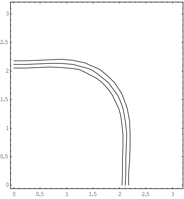
Figure 1: Fermi surfaces for $\mu=-0.1$, $0$, $0.1$ with $t=-0.438$, $t^{\prime}=0.156$, $t^{\prime\prime}=0.098$ where all the energies are represented in eV. Only the quarter of the Brillouin zone ($0<p_{x}<\pi$ and $0<p_{y}<\pi$) is depicted.

The Fermi surface for this dispersion is shown in Fig. 1. The factor $f({\bf p})\equiv v_{x}(v_{x}\partial v_{y}/\partial p_{y}-v_{y}\partial v_{x}/\partial p_{y})$ appearing in $\sigma_{xy}$ is shown in Fig. 2.

For the life-time we adopt the model

$${1\over 2\tau}=w({\bf p})\cdot g_{1}\cdot T+\big{[}1-w({\bf p})\big{]}\cdot g_{2}\cdot T^{2},$$ (7)

similar to the multi-patch model [7] where the Brillouin zone is divided into hot and cold patches. The life-time is determined by the coupling to the anti-ferromagnetic spin-fluctuation. In the cold patches the relevant spin-fluctuation spectrum is broad and its temperature-dependence is weak so that $1/\tau\sim T^{2}$. On the other hand, in the hot patches it is peaked around the nesting-vector and its integrated weight depends on the temperature so that $1/\tau\sim T$. For simplicity we did not implement the gradual change between hot and cold patches employed in [7]. Namely $w({\bf p})$ is a step function in our case where $w({\bf p})=1$ if $({\bf p}-{\bf p}_{1})^{2}<r^{2}$ or $({\bf p}-{\bf p}_{2})^{2}<r^{2}$ with ${\bf p}_{1}\equiv(\pi,0)$ and ${\bf p}_{2}\equiv(0,\pi)$ and $w({\bf p})=0$ otherwise.

We set $g_{2}=100/$eV in accordance with [3]. Here the temperature $T$ is measured in eV. On the other hand, our choice, $g_{1}=0.1$, is smaller than [3] and [7]. Such a smallness is explained by the nested spin fluctuation [8].

Before performing the numerical calculation we can make a rosy prediction that the non-monotonic temperature dependence of $\sigma_{xy}$, which we want to derive, is obtained, if the temperature dependences of $1/\tau$ are different between the regions with positive $f({\bf p})$ and the regions with negative $f({\bf p})$ in the Brillouin zone. After the numerical calculation we confirm the prediction as shown in Fig. 3. The result for $\mu=0$ actually shows the non-monotonic temperature dependence qualitatively similar to that observed in the experiment [4]. More direct comparison between the experiment [4] and our numerical calculation can be done for $\sigma_{xy}/\sigma_{xx}$ shown in Fig. 4.

In conclusion our simple formula based on the relaxation-time approximation for single particles qualitatively explain the non-monotonic behavior of the DC Hall conductivity in the normal state of PCCO superconductors, though our choice of the parameters should be reconsidered for quantitative description.

This work was driven by the discussions with Professor Kazumasa Miyake.

Appendix

In the main text of this Short Note the anomalous behavior of the Hall coefficient in the normal state of high-$T_{c}$ superconductors is explained within the relaxation-time approximation.

In this Appendix how the fluctuation-exchange (FLEX) approximation and the Fermi-liquid theory fail to explain the anomalous behavior of the coefficient (ABC) is clarified.

Let us start with the formulae [5] for $\sigma_{xx}$

$$\sigma_{xx}={4e^{2}\over\pi}\sum_{\bf p}v_{x}^{2}G^{R}G^{A}={4e^{2}\over\pi}\sum_{\bf p}v_{x}^{2}{1\over E^{2}+(1/2\tau)^{2}},$$ (8)

and for $\sigma_{xy}$

$$\sigma_{xy}/H ={4|e|^{3}\over\pi}\sum_{\bf p}v_{x}\Big{(}v_{x}{\partial v_{y}\over\partial p_{y}}-v_{y}{\partial v_{x}\over\partial p_{y}}\Big{)}G^{R}G^{A}{G^{R}-G^{A}\over 2i}$$

$$=-{4|e|^{3}\over\pi}\sum_{\bf p}v_{x}\Big{(}v_{x}{\partial v_{y}\over\partial p_{y}}-v_{y}{\partial v_{x}\over\partial p_{y}}\Big{)}{1/2\tau\over\big{[}E^{2}+(1/2\tau)^{2}\big{]}^{2}}.$$ (9)

Here the propagators $G^{R}$ and $G^{A}$ are expressed in terms of the spectral function $\rho_{\bf p}(\varepsilon)$.

As shown in [5] these formulae lead to the constant Hall coefficient if the spectral function $\rho_{\bf p}(\varepsilon)$ is delta-function-like and isotropic in momentum space. The Fermi-liquid theory for the Hall coefficient [9] also assumes the delta-function-like spectral function so that it also leads to almost temperature-independent Hall coefficient. Thus the Fermi-liquid theory fails to explain the ABC.

The above-mentioned delta-function-like spectral function is justified only for weakly correlated systems. Our calculation in the main text is performed without such a delta-function assumption. We have to use a broad spectral function in a finite momentum space (the 1st Brillouin zone) in the case of strongly correlated system.

Although our spectral function employed in the main text is a simple model, it captures the features of actual one observed by the ARPES experiments. Thus our result for the Hall angle in Fig. 4 qualitatively explains the anomalous non-monotonic temperature dependence observed in experiments. Thus we can conclude that the ABC is explained without the CVC if we employ the correct spectral function.

On the other hand, the Hall angle calculated without the CVC in the FLEX approximation, the inset of Fig. 2 in [4], is totally different from the one observed by experiments. The failure of this calculation does not mean the necessity of the CVC. It only means that the spectral function obtained by the FLEX approximation is incorrect. We have already discussed in arXiv:1301.5996 that the FLEX approximation is not applicable to the system with the Fermi degeneracy.

Consequently, the spectral function is the key to explain the ABC. The FLEX approximation fails to explain the ABC, since the correct spectral function is not obtained by this approximation. The Fermi-liquid theory fails to explain the ABC, since the delta-function assumption is not justified for strongly correlated systems at the room temperature.

This Appendix arose from the two seminars held at the department of physics and the elementary-particle-theory group of Kyushu University. I thank to the organizers of these seminars.

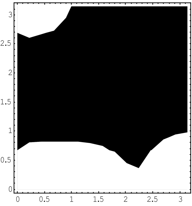
Figure 2: The factor $f({\bf p})=v_{x}(v_{x}\partial v_{y}/\partial p_{y}-v_{y}\partial v_{x}/\partial p_{y})$ in the quarter of the Brillouin zone. In the white region $f({\bf p})>0$ and $f({\bf p})<0$ in the black region.

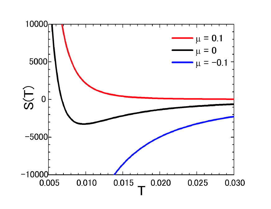
Figure 3: Temperature dependencies of $S(T)$ for $\mu=-0.1$, $0$, $0.1$ with $r^{2}=1.07$ where $S(T)\propto\sigma_{xy}$. The temperature is represented in eV. The summation over ${\bf p}$ is carried out using 3000$\times$3000 mesh in the quarter of the Brillouin zone.

Figure 4: The temperature dependence of $S(T)R(T)$ for $\mu=0$ with $r^{2}=1.07$ where $S(T)R(T)\propto\sigma_{xy}/\sigma_{xx}$.

Figure 5: Energy dependence of spectral function.

References

- [1] P. A. Casey and P. W. Anderson: Phys. Rev. Lett. 106, 097002 (2011).
- [2] J. Kokalj and R. H. McKenzie: Phys. Rev. Lett. 107, 147001 (2011).
- [3] J. Kokalj, N. E. Hussey and R. H. McKenzie: arXiv:1202.4820.
- [4] G. S. Jenkins, D. C. Schmadel, P. L. Bach, R. L. Greene, X. Béchamp-Laganière, G. Roberge, P. Fournier, H. Kontani, and H. D. Drew: Phys. Rev. B 81, 024508 (2010).
- [5] H. Fukuyama, H. Ebisawa, and Y. Wada: Prog. Thoer. Phys. 42, 494 (1969).
- [6] I. A. Nekrasov, E. Z. Kuchinskii, and M. V. Sadovskii: J. Phys. Chem. Solids 72, 371 (2011).
- [7] A. Perali, M. Sindel, and G. Kotliar: Eur. Phys. J. B 24, 487 (2001).
- [8] O. Narikiyo and K. Miyake: Physica C 307, 254 (1998).
- [9] H. Kohno, K. Yamada: Prog. Thoer. Phys. 80, 623 (1988).