Bloch oscillations of quasispin polaritons in a magneto-optically controlled atomic ensemble

Abstract

We consider the propagation of a quantized polarized light in a magneto-optically manipulated atomic ensemble with a tripod configuration. Polariton formalism is applied when the medium is subjected to a washboard magnetic field under electromagnetically induced transparency. The dark-state polariton with multiple components is achieved. We analyze quantum dynamics of the dark-state polariton by some experiment data from rubidium D1-line. It is found that one component propagates freely, however the wavepacket trajectory of the other component performs Bloch oscillations.

I Introduction

Quasiparticles are regarded as collective excitations of many elementary particles, as well as the mixtures of different elementary excitations, which are the basic constructions of matters together with elementary particle. Quasiparticles are crucial for understanding many phenomena in condensed matter physics Firstenberg ; Firstenberg1 . One of the fundamental phenomena in condensed matter physics is the dynamics of particles in a periodic potential under the influence of a static force. As it is well-known that a quantum particle in a periodic potential possesses energy eigenvalues forming Bloch bands and delocalized eigenstates known as Bloch functions, the particle undergoes uniform motion. After a static force is applied, the eigenstates become localized, and the energy spectrum becomes discrete with the formation of Wannier-Stark ladders Wannier60 ; Wacker02 ; Korsch02 . Contrary to common sense, this particle oscillates instead of infinitely accelerating by the force, i.e., the famous Bloch oscillation Bloch28 ; Zener34 . In physics, such an oscillation is generally explained as a Bragg reflection of the accelerated particle, which causes a wave packet to oscillate rather than translate through the lattice.

With the advances of atomic physics and quantum optics over the last decades, considerable attention has been paid on quasiparticles of light-matter interaction since they are suggested as new systems to simulate a variety of many-body phenomena Plenio08 ; Fazio10 with unprecedented precision and control. A prominent phenomenon in light-matter interaction is electromagnetically induced transparency (EIT), where the transmission of a probe beam through an optical dense medium is manipulated by means of a control beam HarrisTD ; RMP77(05)633 . Stimulated by the construction of both quantum memories and quantum carriers free of quantum decoherence, dark state polaritons emerge in storing and transferring quantum state of light to collective atomic excitations of matter in EIT. A dark state polariton (DSP) is a quasiparticle, which is a bosoniclike collective excitation of a photon and an atomic spin wave SunPRL03 ; RMP75(03)457 . The particle nature of dark state polaritons, possessing an effective magnetic moment, has been demonstrated by the enhanced deflection of the laser beam after light propagates through a $\Lambda$-type atomic vapor with a magnetic-field gradient applied PRL78(97)003451 ; Karpa06 , and an effective Schrödinger equation is derived to exhibit the wave-particle duality of the dark state polaritons ZhouA08 . Bloch oscillations of single DSP are proposed ZhangA10 , and a method is described to create an effective gauge potential for a DSP 104(10)033903 .

Another remarkable property of DSPs in EIT is the presence of multiple “spin” components, which open up the possibility to study a variety of many-particle effects in effective magnetic fields. A phenomenon of birefringence in EIT has been predicted as a generalized Stern-Gerlach effect of quantized polarized light yuguoA08 ; ZhangA09 . Collapses and Revivals of DSPs are also experimentally demonstrated KuzmichA06 ; KuzmichL06 . Here, we study spatial motion of the DSP with two components in two inhomogeneous magnetic fields consisting of a periodical magnetic field and a magnetic field gradient. The magnitudes of the magnetic fields vary in a direction transverse to the incident direction of the probe beam. This investigation is inspired by the following technical advantages of DSPs: refractive index modulation straightforwardly creates a scalar potential; a direct measurement is simple for photons; and the waveguide and resonator techniques can be used to confine the spatial motion of polaritons to lower dimensions. In this paper, the DSP with two components is generated in an atomic ensemble with a tripod configuration, which controlled by a specially designed magneto-optical manipulation based on the EIT mechanism. After obtaining the equation of motion for this quasispin DSP by the perturbation theory, we employ the single-band and tight-binding model to give an analytic treatment of the dynamics of DSP. It is found that one DSP component acts as a free particle, the other component experiences a harmonic motion with angular frequency proportional to the steady force and its momentum growing linearly in time (i.e. Bloch oscillations). The experimental feasibility of the proposed scheme is also discussed using rubidium 87 D1-line.

This paper is organized as follows. Section II describes the theoretical model for four-level atoms with a tripod configuration in external fields. In Sec. III, the quasispin DSP has been introduced as dressed fields to describe the spatial motion of collective excitation. Afterward, we present the evolution equation for this quasispin DSP. In Sec. IV, we present the results of detailed calculations for the propagation of the DSP in a washboard magnetic field within single-band and tight-binding approximation. We conclude our paper in the final section.

II Theoretical model for tripod atomic ensemble in external fields.

We deal with an ensemble of 2N identical and noninteracting atoms. Each atom is characterized by three lower states $\{|1\rangle,|2\rangle,|s\rangle\}$, and an excited state $|e\rangle$, as schematically shown in Fig. 1. The two ground states $|1\rangle$ and $|2\rangle$ are the degenerate Zeeman sublevels. Atoms interact with a linear-polarized probe field with frequency $\nu$ and wave vector $\mathbf{k}$ propagating in the positive $z$ direction, and a classical control light with frequency $\nu_{c}$ and wave number $\mathbf{k}_{c}$. Here $k$ and $k_{c}$ are the wave numbers to the central frequencies $\nu$ and $\nu_{c}$ of the probe and control fields, respectively. The excited state $\left|e\right\rangle$ with $m_{F}^{e}=0$ is coupled to the ground state $\left|1\right\rangle$ ($\left|2\right\rangle$) with $m_{F}^{1}=-1$ ($m_{F}^{2}=1$) via a $\sigma^{+}$ ($\sigma^{-}$) component $E_{1}$($E_{2}$) Haun409 ; Lukin86 . The control field with Rabi frequencies $\Omega$ is assumed to be uniform throughout the sample, and it drives the transition $|s\rangle\rightarrow|e\rangle$ with detuning $\delta_{c}$, which create transparent windows for two components of the probe field. We assume that the detuning of component $E_{1}$($E_{2}$) from its corresponding atomic transition is caused by the applied magnetic fields along the $z$ axis with the corresponding amount $\delta_{i}=\mu_{i}B$, the magnetic moments $\mu_{i}=m_{F}^{i}g_{F}^{i}\mu_{B}$ are determined by the Bohr magneton $\mu_{B}$, the gyromagnetic factor $g_{F}^{i}$ and the magnetic quantum number $m_{F}^{i}$ of the corresponding state $\left|i\right\rangle$.

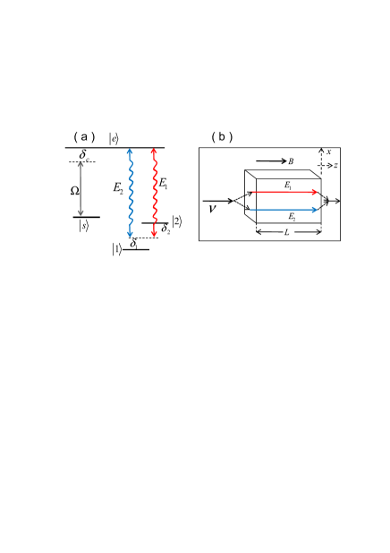
Figure 1: (Color online) Tripod scheme of matter-light interaction involving a linear-polarized probe field and one control field in the presence of a magnetic field parallel to the field propagation direction.

We now introduce components $E_{j}(\mathbf{r},t)$ of the probe field which vary slowly in space and time Lukin1

$$\tilde{E}_{j}^{+}(\mathbf{r},t)=\sqrt{\frac{\nu}{2\varepsilon_{0}V}}E_{j}(\mathbf{r},t)e^{i(kz-\nu t)},(j=1,2)$$ (1)

and slowly varying operators

$$\sigma_{es} = \tilde{\sigma}_{es}\exp(ik_{c}z)\text{,}$$ (2a)

$$\sigma_{ej} = \tilde{\sigma}_{ej}\exp(ikz),(j=1,2)\text{.}$$ (2b)

Here continuous atomic-flip $$\tilde{\sigma}_{\mu\nu}\left(\mathbf{r},t\right)=(1/N_{r})\sum_{r_{j}\in N_{r}}\tilde{\sigma}_{\mu\nu}^{j}\left(t\right) N_{r}=(2N/V)dV\gg 1 \mathbf{r} 2N V \tilde{\sigma}_{\mu\nu}^{j}\left(t\right)=\left|\mu\right\rangle_{j}\langle\nu| \hbar=1$$ is averaged over a small but macroscopic volume containing many atoms around position , where is the total number of atoms, is the volume of the medium Lukin ; Lukin1 , and is the flip operator of the jth atom. Above and hereafter, we take . Under the electric-dipole approximation and the rotating-wave approximation, the interaction Hamiltonian reads

$$H_{I} = \frac{2N}{V}\int d^{3}r\left[\left(\delta_{1}\sigma_{11}+\delta_{2}\sigma_{22}+\delta_{c}\sigma_{ss}\right)\right.$$ (3)

$$\left.-\left(\Omega\sigma_{es}+gE_{1}\sigma_{e1}+gE_{2}\sigma_{e2}+h.c.\right)\right],$$

in a frame rotating with respect to the probe and driving fields. The parameter $g=\langle e|d|1\rangle\sqrt{\nu/(2\varepsilon_{0}V)}$ characterizes the strength of coupling between the probe field and the atoms. Due to the symmetry of the states $|1\rangle$ and $|2\rangle$, the transition matrix elements in the above equation are equal. Although we assume three-photon resonance in the absence of the magnetic field, that is, $\nu=\omega_{e1}^{0}=\omega_{e2}^{0}$, $\nu_{c}=\omega_{es}^{0}$, where $\omega_{e1}^{0}=\omega_{e2}^{0}$ and $\omega_{es}^{0}$ are the atomic resonance frequencies without the applied magnetic field, we note that the interaction Hamiltonian $H_{I}$ is the general expression in the interaction picture for a tripodlike linkage pattern. Here, $\delta_{i}$ $(i=1,2,c)$ is the detuning between the laser field and its corresponding atomic transition.

III Evolution equation for the DSP with two components.

When a light pulse enters a medium, photons interact with atoms of the medium. They are converted into composite quasiparticles of the radiation and atomic excitations known as polaritons. In EIT system, there are two types of polaritons —- the DSP and the bright state polariton. To obtain the equation that describes the dark-state polariton, first we deal with the dynamics of this atomic ensemble. The Heisenberg equations read

$${\dot{\sigma}_{21}} = \left[i\left(\delta_{2}-\delta_{1}\right)-\gamma_{c}\right]\sigma_{21}+ig^{\ast}E_{1}^{+}{\sigma_{2e}}-ig^{\ast}E_{2}^{+}\sigma_{e1},$$ (4a)

$${\dot{\sigma}_{e1}} = \left(-i\delta_{1}-\frac{\Gamma}{2}\right)\sigma_{e1}-ig^{\ast}E_{1}^{+}\left(\sigma_{11}-\sigma_{ee}\right)-ig^{\ast}E_{2}^{+}\sigma_{21}$$ (4b)

$$-i\Omega^{\ast}\sigma_{s2},$$

$${\dot{\sigma}_{s1}} = \left[i\left(\delta_{c}-\delta_{1}\right)-\gamma_{c}\right]\sigma_{s1}+ig^{\ast}E_{1}^{+}\sigma_{se}-i\Omega^{\ast}\sigma_{e1},$$ (4c)

$${\dot{\sigma}_{e2}} = \left(-i\delta_{2}-\frac{\Gamma}{2}\right)\sigma_{e2}-ig^{\ast}E_{2}^{+}\left(\sigma_{22}-\sigma_{ee}\right)-ig^{\ast}E_{1}^{+}\sigma_{12}$$ (4d)

$$-i\Omega^{\ast}\sigma_{s2},$$

$${\dot{\sigma}_{s2}} = \left[i\left(\delta_{c}-\delta_{2}\right)-\gamma_{c}\right]\sigma_{s2}+ig^{\ast}E_{2}^{+}\sigma_{se}-i\Omega\sigma_{e2},$$ (4e)

$${\dot{\sigma}_{se}} = \left(i\delta_{c}-\frac{\Gamma}{2}\right)\sigma_{se}+ig^{\ast}E_{1}\sigma_{s1}-ig^{\ast}E_{2}\sigma_{s2}$$ (4f)

$$-i\Omega\left(\sigma_{ee}-\sigma_{ss}\right),$$

where we have phenomenologically introduced the coherence relaxation rate $\gamma_{c}$ of the ground states and the decay rate $\Gamma$ of the excited state. Here, we consider the case where the intensity of the quantum field is much weaker than that of the coupling field, and the number of photons contained in the signal pulse is much less than the number of atoms in the sample. Therefore, the perturbation approach can be applied to the Heisenberg equations of the atomic part of the order in $gE_{j}$, which is introduced in terms of perturbation expansion

$$\sigma_{\mu\nu}=\sigma^{(0)}_{\mu\nu}+\lambda\sigma^{(1)}_{\mu\nu}+\cdots$$ (5)

In the above equation, $\mu,\nu\in\{1,2,s,e\}$ and $\lambda$ is a continuously varying parameter ranging from zero to unity. Here, $\sigma^{(0)}_{\mu\nu}$ is of the zeroth order in $gE_{j}$ and $\sigma^{(1)}_{\mu\nu}$ is of the first order in $gE_{j}$, and so on. We retain only terms up to the first order in the signal field amplitude since the linear optical response theory can sufficiently reflect the main physical features of the spatial motion of the input pulse with slow group velocity. With the assumption that all atoms are initially in level $|j\rangle,(j=1,2)$ without polarization, i.e., atom $i$ is in a mix state $\rho_{i}=\Sigma_{j=1,2}|j\rangle\langle j|/2$, we can neglect the population of states $|e\rangle$ and $|s\rangle$, as well as the coherence between these states. Then the first order atomic transition operator $\sigma_{ij}^{(1)}$ satisfies the following equation

$$\sigma_{je}^{\left(1\right)}=-\frac{i}{\Omega^{\ast}}\left(\partial_{t}-d_{j}\right)\sigma_{js}^{\left(1\right)},$$ (6)

which is related to the atomic linear response to the probe field. In the above equation,

$$d_{j}=i\left(\delta_{j}-\delta_{c}\right)-\gamma_{c},$$

The dark-state and bright-state polaritons are described by the field operators as

$$\Psi_{j} = E_{j}\cos\theta-2\sqrt{N}\sigma_{js}^{(1)}\sin\theta\text{,}$$ (7a)

$$\Phi_{j} = E_{j}\sin\theta+2\sqrt{N}\sigma_{js}^{(1)}\cos\theta\text{,}$$ (7b)

respectively, which are superpositions of photonic and spin-wave excitations. They are introduced in the linear regime with respect to the probe field. Here, $\tan\theta=g\sqrt{N}/\Omega$. The Heisenberg equation for the slowly varying field operator $E_{j}(\mathbf{r},t)$ results in a paraxial wave equation in classical optics

$$\left[i\partial_{t}+ic\partial_{z}+\frac{c}{2k}(\frac{\partial^{2}}{\partial x^{2}}+\frac{\partial^{2}}{\partial y^{2}})\right]E_{j}=-2g^{\ast}N\sigma_{je}^{(1)}.$$ (8)

Here, $c$ is the velocity of light in vacuum. In terms of dark and bright polariton field operators, equations (6) and (8) read ZhouA08 ; yuguoA08

$$\left[i\partial_{t}+ic\partial_{z}+\frac{c}{2k}\left(\partial_{x}^{2}+\partial_{y}^{2}\right)\right]\left(\Psi_{j}\cos\theta+\Phi_{j}\sin\theta\right)$$

$$= i\frac{g^{\ast}\sqrt{N}}{\Omega^{\ast}}\left(\partial_{t}-d_{j}\right)\left(\Phi_{j}\cos\theta-\Psi_{j}\sin\theta\right).$$ (9)

Under the condition of EIT, absorption is negligible, the excitation of the bright-state polariton field $\Phi_{j}$ vanishes approximately. Then the dynamics of dark-state polariton field $\Psi_{j}$ is obtained. To show the basic principle of physics, we assume a sufficiently strong driving field such that $\left|\Omega\right|^{2}\gg\Gamma\gamma_{c}$. In addition, we have let $\gamma_{c}=0$. To make an analogy to the schrödinger equation, we rewrite the dynamic equation for the two dark-state polaritons as

$$i\partial_{t}\Psi_{j}=\left[v_{g}P_{z}+\frac{P_{x}^{2}+P_{y}^{2}}{2m}+\mu_{j}^{eff}B(x)\right]\Psi_{j},$$ (10)

Here, effective magnetic moments

$$\mu_{j}^{eff}=(\mu_{s}-\mu_{j})\sin^{2}\theta,$$

which can be adjusted by the control field. In addition, the group velocity $v_{g}=c\cos^{2}\theta$ along the $z$ direction can be controlled by the amplitude of the control field. $m=k/{v_{g}}$ is the effective mass, and $P_{\alpha}=-i\partial_{\alpha}(\alpha=x,y,z)$ is the momentum operator on the $\alpha$ direction yuguoA08 . The steady atomic response in the applied magnetic fields induces an effective potential for the DSP. Equation (10) indicates that the two components of a DSP behave independently, i.e. two components of a DSP does not interact with each other. Now, we assume that the magnetic fields in z direction consist of two components, one is linear with the expression $B_{1}x$ and the other is periodical in the transverse $x$ direction. Then the treatment proceeds along the $x-z$ plane. The evolution equation for the quasispin DSP is rewritten as

$$i\partial_{t}\Psi_{j}=\left[v_{g}P_{z}+\frac{P_{x}^{2}}{2m}+F_{j}x+V_{j}(x)\right]\Psi_{j},$$

which means each component $\Psi_{j}$ is subject to a static force $F_{j}=\mu_{j}^{eff}B_{1}$ in its corresponding periodic potential $V_{j}(x+d)=V_{j}(x)$. Since the effective Hamiltonian along $z$ direction commutes with that along the transverse direction which refers to Wannier-Stark Hamiltonian Korsch02 , therefore, the investigation is confined to the transverse direction. We note that the evolution operator along $z$-axis is equivalent to the translation operator, and the Hermitian of the Wannier-Stark Hamiltonian preserves the number of the particle along $x$ direction.

IV Quantum dynamics of a quasispin dark state polariton

To show the possibility that the dynamics of DSP mirrors the Bloch oscillation in this atom–photon system, we consider the atomic medium with light tuned to the rubidium (⁸⁷Rb) D1-line $5^{{}^{2}}S_{{}_{1/2}}\leftrightarrow 5^{{}^{2}}P_{{}_{1/2}}$ as shown in Fig. 2(a). The ground states contain two hyperfine ground levels with $F=1$ and $F=2$, where $\left|1\right\rangle$ and $\left|2\right\rangle$ correspond to the magnetic sublevels (with $m_{F}=1$ and $-1$) of the $F=1$ hyperfine ground state and $\left|s\right\rangle$ represents the hyperfine ground state $\left|F=2,m_{F}=1\right\rangle$. In this case, the effective magnetic moment $\mu_{1}^{eff}$ vanishes due to $\mu_{s}=\mu_{1}$, which leads to the free propagation of the component $\Psi_{1}$. Therefore, a wave packet with a Gaussian profile in space

$$\Psi_{1}\left(x,z,0\right)=\prod_{\alpha=x,z}\frac{1}{\sqrt[4]{2\pi\sigma_{\alpha}^{2}}}e^{-\frac{\alpha^{2}}{4\sigma_{\alpha}^{2}}}$$ (11)

at the initial time, will keep its shape in all directions. Since equation (11) has a pronounced peak with width $\sigma_{x}$ situated at moment $p_{x}=0$, the wave-packet will always localize around the position $x=0$ along x-axis, but the center of the wave-packet in $z$-direction moves to $z=v_{g}t$.

Figure 2: (Color online) A possible experimental realization of the tripod scheme in matter-light system in rubidium 87 (a) and an illustration of the periodical potential for the second component of DSP induced by the periodical magnetic field (b).

Different from $\Psi_{1}$, the second component $\Psi_{2}$ feels potentials due to its nonzero effective magnetic moment. Obviously, in the absence of the linear magnetic field, the period potential gives rise to the Bloch bands. To make this discussion more quantitative, we assume that $V_{2}\left(x\right)$ is the Kroning-Penney potential which is formed by a periodic sequence of rectangular wells with amplitude $V_{0}=79.15kHz$. As illustrated in Fig. 2(b), the lattice constant of the periodic array $d=8\mu m$ is equal to $a+b$. Within the unit cell, the barrier region $0<x<a$, the well region $-b<x<0$. By taking the effective transverse mass $m=7.9\times 10^{5}sm^{-2}$ for the wavelength of the probe field $\lambda=795nm$, we obtain the width $\Delta=74.9kHz$ of the ground energy band, and the gap interval $E_{g}=266kHz$ between two lower bands. For a linear magnetic field with magnitude $B_{1}=8.5\times 10^{4}\mu Gmm^{-1}$, the magnetic moments $\mu_{2}=-4.64\times 10^{-24}JT^{-1}$ and $\mu_{s}=4.64\times 10^{-24}JT^{-1}$ allow us to find that $F_{2}d\ll E_{g}$. So the ground band is well separated and one can neglect the interband mixing induced by the static force $F_{2}$. By assuming that neighboring wells are directly coupled, the dynamics of the DSP component $\Psi_{2}$ is described by the Hamiltonian

$$H_{1}=\frac{-\Delta}{4}\sum_{n}\left(\left|n\right\rangle\left\langle n+1\right|+h.c.\right)+dF_{2}\sum_{n}n\left|n\right\rangle\left\langle n\right|$$

in terms of Wannier state $\left|n\right\rangle$, which is localized around position $x=nd$. It is useful to introduce the eigenstates $\left|\kappa\right\rangle$ (Bloch states) of Hamiltonian $H_{1}$ with $F_{2}=0$,

$$\left|\kappa\right\rangle=\sqrt{\frac{d}{2\pi}}\sum_{n}\left|n\right\rangle e^{in\kappa d}$$ (13)

which is the Fourier transform of the Wannier states. The tight-binding Hamiltonian in Eq.(IV) is diagonalized as

$$H_{1}\left(k\right)=-\frac{\Delta}{2}\cos\left(\kappa d\right)+iF_{2}\frac{d}{d\kappa}$$ (14)

in the quasi-momentum representation with the quasi-momentum $\kappa\in\left[-\pi/d,\pi/d\right]$ in the first Brillouin zone. Diagonalizing $H_{1}$ gives the Wannier-Stark ladder with energies $E_{m}=mdF_{2}$, where $m$ is an integer. The Wannier–Stark state $\left|\psi_{m}\right\rangle$ to the eigenvalue $E_{m}$ is given by

$$\left|\psi_{m}\right\rangle=\sqrt{\frac{d}{2\pi}}\int d\kappa e^{-i\left[\Delta\sin\left(\kappa d\right)/\left(2dF_{2}\right)+md\kappa\right]}\left|\kappa\right\rangle$$ (15)

In the Wannier-state representation, we obtain

$$\left|\psi_{m}\right\rangle=\sum_{n}J_{n-m}\left(\frac{\Delta}{2dF_{2}}\right)\left|n\right\rangle$$ (16)

where $J_{n-m}$ is the Bessel functions of the first kind and of integer order $n-m$.

To show the wave-particle duality of the second DSP component, we now discuss the quantum dynamics under the assumption that an initially Gaussian wave packet

$$\left|\varphi\left(0\right)\right\rangle=\sum_{n}\left(\frac{d^{2}}{2\pi\sigma^{2}}\right)^{1/4}\exp\left[-\frac{n^{2}d^{2}}{4\sigma^{2}}\right]\left|n\right\rangle$$ (17)

is launched into the lattice with a center value at $x_{0}=0$ and width $\sigma$. Since the time-evolution operator is diagonal in Wannier–Stark states, each element $U_{\mu\nu}\equiv\left\langle\mu\right|U\left(t\right)\left|\nu\right\rangle$ of the time-evolution operator $U\left(t\right)$ in the Wannier-state representation has the form

$$U_{\mu\nu}=J_{\nu-\mu}\left(\frac{\Delta\sin\alpha}{\omega_{{}_{B}}}\right)e^{-i\mu\omega_{{}_{B}}t}e^{-i\left(\nu-\mu\right)\left(\omega_{{}_{B}}t-\pi\right)/2},$$ (18)

where $\alpha=\omega_{{}_{B}}t/2$ and $\omega_{{}_{B}}=dF_{{}_{2}}$. The argument of $J_{\nu-\mu}$ oscillates in time. The state at arbitrary time can be expressed as $\left|\varphi\left(t\right)\right\rangle=\sum_{n}f_{n}\left(t\right)\left|n\right\rangle$. As the Gaussian wave packet is broad initially, i.e. $\sigma/d$ $\gg 1$, the coefficient $f_{n}\left(t\right)$ is approximately given by

$$f_{n}\left(t\right)=\frac{e^{-d^{2}\left(n-n_{t}\right)^{2}/4\sigma^{2}}}{\sqrt[4]{2\pi\sigma^{2}/d^{2}}}e^{-in\omega_{{}_{B}}t+i\Delta\sin\left(\omega_{{}_{B}}t\right)/(2\omega_{{}_{B}})}$$ (19)

where $n_{t}=x_{c}\left(t\right)/d$. Here, the motion of the wave packet center along $x$-direction

$$x_{c}\left(t\right)=\frac{\Delta}{2F_{2}}\left[\cos\left(\omega_{{}_{B}}t\right)-1\right]$$ (20)

reduces the quantum mechanical dynamics to the classical trajectories. Equation (20) implies that the DSP component $\Psi_{2}$ experiences a harmonic motion around the initial position $x_{0}$ with angular frequency $\omega_{{}_{B}}$ and amplitude $A=\Delta/\left(2F_{2}\right)$. As expected from the semiclassical picture, the band width $\Delta$ equals the product of the total spatial extension $2A$ and the static force $F_{2}$. Besides the trajectory of the wave packet, equation (19) also gives a description on the variation of the particle’s wavenumber $\kappa=\omega_{{}_{B}}t/d=F_{{}_{2}}t$ in the semiclassical picture. Since $z=v_{g}t$ is the relation between the center of the wave packet along the z direction and the time, we achieve the spatial Bloch oscillation

$$x\left(z\right)=A\left[1-\cos\left(\zeta z\right)\right]$$

with spatial period $2\pi/\zeta$. Here, $\zeta=dF_{2}/v_{g}$.

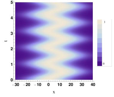
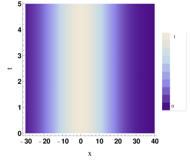
Figure 3: (Color online) Density plots of the norm square of the wave function for a DSP with two components arising from an extended Gaussian distribution. The probabilities for the components $\Psi_{2}$ (a) and $\Psi_{1}$ (b) is plot as a function of x in units of lattice constant $d$ and t in units of millisecond, where the initial states for both components are taken to be the same with width $0.1$mm.

In Fig. 3, we plot the probabilities for the components $\Psi_{1}$ and $\Psi_{2}$ versus $x/d$ and $t$, where the initial states of both components are identical broad Gaussian wave packets. One can see that two components behave differently in the transverse direction though the wave packets for both components keeps it shape along z direction with an unchanged variance. The trajectory of component $\Psi_{1}$ is always localized at its initial position, which means this component appears like a free particle. However, component $\Psi_{2}$ presents a back and forth behavior around an equilibrium point with a constant amplitude and a constant frequency, so it acts as a particle moving through a quadratic potential.

V Conclusion

We study an optical-controlled cloud of identical atoms in a washboard magnetic field applied along $z$-direction. The probe and control laser beams drive three hyperfine ground states to a common excited state, which form a tripod configuration. The quasispin DSP is excited in the EIT condition. The equation for the space-time evolution of this quasispin DSP shows that each component is subject to its corresponding effective potential induced by the steady atomic response in the external spatial-dependent field. By taking the value of parameters from the experiment data in rubidium D1-line, it is found that one component $\Psi_{1}$ of the DSP acts as a free particle. The behavior of the other component $\Psi_{2}$ is analyzed via the single band and tight-binding approximation. By considering the time evolution of the broad Gaussian state for the component $\Psi_{2}$, the particle nature of component $\Psi_{2}$ is shown by the trajectory of the wavepacket, which undergoes a periodic motion with angular frequency proportional to the steady force. Besides, its momentum grows linearly in time. This periodic motion is termed as Bloch oscillations. The oscillation amplitude and period are controlled by the intensity of the control field and the magnitude of the magnetic fields.

It should be pointed out that there are many differences between our present scheme and that in Ref. ZhangA10 : 1) The atomic configurations are different. Lambda type is studied in Ref. ZhangA10 , however tripod pattern is studied in our manuscript. From the technical point of view, tripod atoms proved to be robust systems for “engineering” arbitrary coherent superpositions of atomic states VewPRL91 using an extension of the well known technique of stimulated Raman adiabatic passage. 2) The double-EIT effect has been used in our manuscript. Double EIT is an important phenomenon for quantum information processing and quantum computing. 3) In our paper, different types of dark polaritons are demonstrated to possess different effective magnetic moments. 4) The predicted phenomena in our manuscript are more general. It could be found that only one dark polariton is excited in Ref. ZhangA10 , so only one trajectory is found inside the atomic medium. However, in our paper, two dark polaritons are excited by one probe beam and a spatial bifurcation and dynamics of these dark polaritons is obtained inside the atomic medium. 5) Our approach naturally shows the multiple degrees of freedom of photons and the role of quantum coherence. As one can find that when the single photon with a superposition of two orthogonal components of polarization is incident on the atomic medium, one obtain a superposition state of two DSPs relating to different spin-states of this incident single photon. Besides, our investigation provides a way to control the dynamics of DSPs. In addition to the external fields, atomic energy levels can be used as a way to adjust the motion of DSP, for example, one can choose the atomic energy level to make the DSP have vanished effective magnetic moment. The presence of the first component unaffected by the washboard potential might be used to eliminate the distortions or aberrations in future.

This work is supported by the Program for New Century Excellent Talents in University (NCET-08-0682), NSFC No. 11105050, and No. 11074071, NFRPC 2012CB922103, PCSIRT No. IRT0964, the Key Project of Chinese Ministry of Education (No. 210150), the Research Fund for the Doctoral Program of Higher Education No. 20104306120003, Hunan Provincial Natural Science Foundation of China(11JJ7001), and Scientific Research Fund of Hunan Provincial Education Department (No. 11B076).We thanks H. R. Zhang for useful discussions.

References

- (1) O. Firstenberg, M. Shuker, N. Davidson, and A. Ron, Pys. Rev. Lett. 102, 043601 (2009).
- (2) O. Firstenberg, M. Shuker, A. Ron, and N.Davidson, Nature Phys. 5, 665 (2009).
- (3) G.H. Wannier, Phys. Rev. 117, 432 (1960).
- (4) Andreas Wacker, Phys. Rep. 357, 1 (2002).
- (5) M. Glück, A.R. Kolovsky, and H.J. Korsch Phys. Rep. 366 103 (2002)
- (6) F. Bloch, Z. Phys. 52, 555(1928).
- (7) C. Zener, Proc. R. Soc. London, Ser. A 145, 523 (1934).
- (8) M. J. Hartmann, F. G. S. L. Brandao, and M. B. Plenio, Laser & Photon. Rev. 2, 527 (2008).
- (9) A. Tomadin and R. Fazio, J. Opt. Soc. Am. B 27, A130 (2010). Also arXiv:1005.0137.
- (10) Harris, S. E. Electromagnetically induced transparency. Phys. Today 50, 36 (1997).
- (11) M. Fleischhauer, A. Imamoglu, and J. P. Marangos, Rev. Mod. Phys. 77, 633 (2005)
- (12) C. P. Sun, Y. Li, and X. F. Liu, Phys. Rev. Lett. 91, 147903 (2003)
- (13) M. D. Lukin, Rev. Mod. Phys. 75, 457 (2003).
- (14) R. Holzner, P. Eschle, S. Dangel, et al., Phys. Rev. Lett. 78, 3451 (1997).
- (15) L. Karpa and M. Weitz, Nat. Phys. 2, 332 (2006).
- (16) L. Zhou, J. Lu, D. L. Zhou, and C. P. Sun, Phys. Rev. A 77, 023816 (2008).
- (17) H. R. Zhang and C. P. Sun, Phys. Rev. A 81, 063427 (2010).
- (18) J. Otterbach, J. Ruseckas, R. G. Unanyan, G. Juzeli ūnas, and M. Fleischhauer, Phys. Rev. Lett. 104, 033903 (2010).
- (19) Y. Guo, L. Zhou, L. M. Kuang, and C. P. Sun, Phys. Rev. A 78, 013833 (2008).
- (20) H. R. Zhang, Lan Zhou, and C. P. Sun, Phys. Rev. A 80, 013812 (2009).
- (21) S. D. Jenkins, D. N. Matsukevich, T. Chanelière, A. Kuzmich, and T. A. B. Kennedy, Phys. Rev. A 73, 021803 (2006).
- (22) D. N. Matsukevich, T. Chanelière, S. D. Jenkins, S.-Y. Lan, T. A. B. Kennedy, and A. Kuzmich, Phys. Rev. Lett. 96, 033601 (2006).
- (23) C. Liu, Z.Dutton, C. H. Behoozi, and L.V. Hau, Nature (London) 409, 490 (2001).
- (24) D. F. Phillips, A. Fleischhauer, A. Mair, R. L. Walsworth, and M. D. Lukin, Phys. Rev. Lett. 86, 783 (2001).
- (25) M. Fleischhauer and M. D. Lukin, Phys. Rev. A 65, 022314 (2002).
- (26) M. Fleischhauer and M. D. Lukin, Phys. Rev. Lett. 84, 5094 (2000).
- (27) F. Vewinger, M. Heinz, R.G. Fernandez, N.V. Vitanov, and K. Bergmann, Phys. Rev. Lett. 91, 213001 (2003)