Compact Finite Difference Approximations for Space Fractional Diffusion Equations

Abstract

Based on the weighted and shifted Grünwald difference (WSGD) operators [24], we further construct the compact finite difference discretizations for the fractional operators. Then the discretization schemes are used to approximate the one and two dimensional space fractional diffusion equations. The detailed numerical stability and error analysis are theoretically performed. We theoretically prove and numerically verify that the provided numerical schemes have the convergent orders $3$ in space and $2$ in time.

Keywords: Compact difference approximation, Fractional operator, Stability and convergence, Space fractional diffusion equation.

AMS subject classifications: 65M06, 26A33, 65M12, 35R11.

1 Introduction

Diffusion is a fundamental phenomena in real world. The classical diffusion equation can be derived from the conservation law of particles, when assuming the particles’ diffusion satisfies the Fick’s law. Based on the CTRW model of statistical physics, it can also be easily derived. Nowadays, anomalous diffusion is widely recognized in scientific community, its basic feature is that the classical Fick’s law doesn’t not hold again. In fact, anomalous diffusion is usually characterized by the mean square displacement of the particles, given by $\langle x^{2}(t)\rangle-\langle x(t)\rangle^{2}\sim t^{\alpha}$. The exponent $\alpha$ classifies the type of diffusion: for $\alpha=1$, we have normal diffusion; for $0<\alpha<1$, subdiffusion; and $\alpha>1$, superdiffusion. The anomalous diffusion equations can still be derived from two ways: using the conservation law and fractional Fick’s law; and from the CTRW model with power law waiting time and/or power law jump length distribution. Fractional calculus plays an important role in obtaining the anomalous diffusion equations [1, 2, 3, 4, 10, 11, 19, 25].

The equation describing the superdiffusion is the space fractional diffusion equation, and its concrete form is to replace the second order derivative of the classical diffusion equation by the Riemann-Liouville fractional derivative of order $\alpha$ and $1<\alpha<2$ [10, 11]. This paper concerns the high accurate numerical methods for the space fractional diffusion equation. Meerschaert and his collaborators first introduce the shifted Grünwald formula and successfully get the stable finite difference scheme for numerically solving the space fractional equation based on this formula [12]. Later more research works are appeared by using the shifted Grünwald formula to discretize the space fractional derivatives [8, 12, 13, 14] with first order accuracy in space, and possibly obtaining second order accuracy after extrapolation [21, 22]. In [24], the weighted and shifted Grünwald difference (WSGD) operators are introduced to discretize the fractional operators with second or higher order accuracy, then the second order finite difference schemes are established to numerically solve the space fractional diffusion equation. In [24], it is also verified that the 3-WSGD operator can approximate the Riemann-Liouville fractional derivative with third order accuracy, but the 3-WSGD operator fails to numerically solve the time dependent space fractional diffusion equations with unconditional stability.

As the sequel to [24], based on the WSGD operators we focus on constructing the compact finite difference discretizations, termed compact WSGD operators (CWSGD), for the fractional operators with third order accuracy. When the order of fractional derivative $\alpha$ equals to $1$ or $2$, it becomes the compact difference operators for the first or second order spatial derivatives with fourth order accuracy, which have been widely used in numerically solving the linear and nonlinear, steady and evolution equations to achieve the high order accuracy [7, 17, 20, 23]. By using the CWSGD operator, we get the third order numerical schemes for the space fractional diffusion equation. We theoretically make the numerical stability and error analysis, and the detailedly numerical experiments confirm the theoretical results. In performing the theoretical analysis, the negative definite property of the matrix generated by the WSGD discretization to the fractional diffusion operator [24] still plays a key role.

This paper is organized as follows. In Sec. 2, we introduce the CWSGD operators. Based on the CWSGD operators, in Sec. 3 and 4, we build the compact finite difference schemes for the one and two dimensional space fractional diffusion equations. The stability and third order convergence with respect to the discrete $L^{2}$ norm of the difference schemes are proven. In Sec. 5, the extensive numerical experiments are performed to verify the accuracy and theoretical convergent order. And some concluding remarks are made in the last section.

2 Compact WSGD Operators for the Riemann-Liouville Fractional Derivatives

Now from the WSGD operator and the Taylor’s expansions of the shifted Grünwald finite difference formulae, we derive the CWSGD operators for the Riemann-Liouville derivatives. First let us introduce the definition of the Riemann-Liouville derivatives.

Definition 1 ([15]).

The $\alpha\,(n-1<\alpha<n)$ order left and right Riemann-Liouville fractional derivatives of the function $u(x)$ on $(a,b)$ are, respectively, defined as

• left Riemann-Liouville fractional derivative:

  $${}_{a}D_{x}^{\alpha}u(x)=\frac{1}{\Gamma(n-\alpha)}\frac{\mathrm{d}^{n}}{\mathrm{d}x^{n}}\int_{a}^{x}\frac{u(\xi)}{(x-\xi)^{\alpha-n+1}}\mathrm{d}\xi;$$

• right Riemann-Liouville fractional derivative:

  $${}_{x}D_{b}^{\alpha}u(x)=\frac{(-1)^{n}}{\Gamma(n-\alpha)}\frac{\mathrm{d}^{n}}{\mathrm{d}x^{n}}\int_{x}^{b}\frac{u(\xi)}{(\xi-x)^{\alpha-n+1}}\mathrm{d}\xi;$$

if $\alpha=n$, then ${}_{a}D_{x}^{\alpha}u(x)=\frac{\mathrm{d}^{n}}{\mathrm{d}x^{n}}u(x)$ and ${}_{x}D_{b}^{\alpha}u(x)=(-1)^{n}\frac{\mathrm{d}^{n}}{\mathrm{d}x^{n}}u(x)$.

The second order finite difference approximations (the WSGD operators) for Riemann-Liouville fractional derivatives are given as follows.

Lemma 1 ([24]).

Let $u\in L^{1}(\mathbb{R})$, ${}_{-\infty}D_{x}^{\alpha+2}u$, ${}_{x}D_{\infty}^{\alpha+2}u$ and their Fourier transformations belong to $L^{1}(\mathbb{R})$, and define the weighted and shifted Grünwald difference (WSGD) operators by

$${{}_{L}}\mathcal{D}_{h,p,q}^{\alpha}u(x)=\frac{1}{h^{\alpha}}\sum_{k=0}^{\infty}g_{k}^{(\alpha)}\Big{(}\frac{\alpha-2q}{2(p-q)}u(x-(k-p)h)+\frac{2p-\alpha}{2(p-q)}u(x-(k-q)h)\Big{)},$$ (2.1a)

$${{}_{R}}\mathcal{D}_{h,p,q}^{\alpha}u(x)=\frac{1}{h^{\alpha}}\sum_{k=0}^{\infty}g_{k}^{(\alpha)}\Big{(}\frac{\alpha-2q}{2(p-q)}u(x+(k-p)h)+\frac{2p-\alpha}{2(p-q)}u(x+(k-q)h)\Big{)},$$ (2.1b)

where $g_{k}^{(\alpha)}=(-1)^{k}\binom{\alpha}{k}$ are the coefficients of the power series of the function $(1-z)^{\alpha}$, and $p,q$ are integers, $p\neq q$. Then we have

$${{}_{L}}\mathcal{D}_{h,p,q}^{\alpha}u(x)={{}_{-\infty}}D_{x}^{\alpha}u(x)+O(h^{2}),$$ (2.2a)

$${{}_{R}}\mathcal{D}_{h,p,q}^{\alpha}u(x)={{}_{x}}D_{\infty}^{\alpha}u(x)+O(h^{2}),$$ (2.2b)

uniformly for $x\in\mathbb{R}$.

From [21], we know that the Taylor’s expansions of the shifted Grünwald finite difference formulae, which is necessary for establishing the CWSGD operator for Riemann-Liouville fractional derivatives.

Lemma 2 ([21]).

Assuming that $u\in C^{n+3}(\mathbb{R})$ such that all derivatives of $u$ up to order $n+3$ belong to $L^{1}(\mathbb{R})$, then for any nonnegative integer $p$, we can obtain that

$$\frac{1}{h^{\alpha}}\sum_{k=0}^{\infty}g_{k}^{(\alpha)}u(x-(k-p)h)={{}_{-\infty}}D_{x}^{\alpha}u(x)+\sum_{l=1}^{n-1}\Big{(}a^{\alpha}_{p,l}~{}{{}_{-\infty}}D_{x}^{\alpha+l}u(x)\Big{)}h^{l}+O(h^{n}),$$ (2.3a)

$$\frac{1}{h^{\alpha}}\sum_{k=0}^{\infty}g_{k}^{(\alpha)}u(x+(k-p)h)={{}_{x}}D_{\infty}^{\alpha}u(x)+\sum_{l=1}^{n-1}\Big{(}a^{\alpha}_{p,l}~{}{{}_{x}}D_{\infty}^{\alpha+l}u(x)\Big{)}h^{l}+O(h^{n}),$$ (2.3b)

uniformly for $x\in\mathbb{R}$, where $a^{\alpha}_{p,l}$ are the coefficients of the power series expansion of function $w_{\alpha,p}(z)=\Big{(}\frac{1-e^{-z}}{z}\Big{)}^{\alpha}e^{pz}$, and $w_{\alpha,p}(z)=\sum\limits_{k=0}^{\infty}a^{\alpha}_{p,k}z^{k}=1+(p-\frac{\alpha}{2})z+\frac{1}{24}(\alpha+3\alpha^{2}-12\alpha p+12p^{2})z^{2}+O(z^{3})$.

For any function $u(x)$, denoting by $\delta_{x}^{2}$ the second order central difference operator, that is $\delta_{x}^{2}u(x)=\big{(}u(x-h)-2u(x)+u(x+h)\big{)}/h^{2}$, we introduce the following finite difference operator

$$\mathcal{C}_{x}u=(1+c_{p,q,2}^{\alpha}h^{2}\delta_{x}^{2})u,$$ (2.4)

where $c_{p,q,2}^{\alpha}=\frac{\alpha-2q}{2(p-q)}a_{p,2}^{\alpha}+\frac{2p-\alpha}{2(p-q)}a_{q,2}^{\alpha}$. We call $\mathcal{C}_{x}$ the CWSGD operator of Riemann-Liouville fractional derivatives, of which the detailed construction is described in the following proposition.

Proposition 1.

Under the conditions of Lemmas 1 and 2, there exist

$$\begin{split}&{{}_{L}}\mathcal{D}_{h,p,q}^{\alpha}u(x)=\mathcal{C}_{x}~{}\Big{(}{{}_{-\infty}}D_{x}^{\alpha}u(x)\Big{)}+c_{p,q,3}^{\alpha}~{}{{}_{-\infty}}D_{x}^{\alpha+3}u(x)h^{3}+O(h^{4}),\\ &{{}_{R}}\mathcal{D}_{h,p,q}^{\alpha}u(x)=\mathcal{C}_{x}~{}\Big{(}{{}_{x}}D_{\infty}^{\alpha}u(x)\Big{)}+c_{p,q,3}^{\alpha}~{}{{}_{x}}D_{\infty}^{\alpha+3}u(x)h^{3}+O(h^{4}),\end{split}$$ (2.5)

uniformly for $x\in\mathbb{R}$, where $p,q$ are nonnegative integers and $p\neq q$. The operator $\mathcal{C}_{x}$ is defined in 2.4.

Proof.

Substituting formulae 2.3a and 2.3b into 2.1a and 2.1b, respectively, and taking $n=4$, we arrive at

$$\begin{split}&{{}_{L}}\mathcal{D}_{h,p,q}^{\alpha}u(x)=\Big{(}1+c_{p,q,2}^{\alpha}h^{2}\frac{\mathrm{d}^{2}}{\mathrm{d}x^{2}}\Big{)}\big{(}{{}_{-\infty}}D_{x}^{\alpha}u(x)\big{)}+c_{p,q,3}^{\alpha}~{}{{}_{-\infty}}D_{x}^{\alpha+3}u(x)h^{3}+O(h^{4}),\\ &{{}_{R}}\mathcal{D}_{h,p,q}^{\alpha}u(x)=\Big{(}1+c_{p,q,2}^{\alpha}h^{2}\frac{\mathrm{d}^{2}}{\mathrm{d}x^{2}}\Big{)}\big{(}{{}_{x}}D_{\infty}^{\alpha}u(x)\big{)}+c_{p,q,3}^{\alpha}~{}{{}_{x}}D_{\infty}^{\alpha+3}u(x)h^{3}+O(h^{4}).\end{split}$$ (2.6)

Since $\delta_{x}^{2}u=\frac{\mathrm{d}^{2}}{\mathrm{d}x^{2}}u+O(h^{2})$, it yields

$$\mathcal{C}_{x}u=(1+c_{p,q,2}^{\alpha}h^{2}\frac{\mathrm{d}^{2}}{\mathrm{d}x^{2}})u+O(h^{4}).$$ (2.7)

Then we obtain the needed results by substituting 2.7 into 2.6. ∎

Remark 1.

If the function $u(x)$ is defined on the bounded interval $[a,b]$ with boundary condition $u(a)=0$ or $u(b)=0$, then the WSGD formulae approximating the $\alpha$ order left and right Riemann-Liouville fractional derivatives of $u(x)$ at each point x are written as

$$\begin{split}&{{}_{L}}\mathcal{D}_{h,p,q}^{\alpha}u(x)=\frac{\mu_{1}}{h^{\alpha}}\sum_{k=0}^{[\frac{x-a}{h}]+p}g_{k}^{(\alpha)}u(x-(k-p)h)+\frac{\mu_{2}}{h^{\alpha}}\sum_{k=0}^{[\frac{x-a}{h}]+q}g_{k}^{(\alpha)}u(x-(k-q)h),\\ &{{}_{R}}\mathcal{D}_{h,p,q}^{\alpha}u(x)=\frac{\mu_{1}}{h^{\alpha}}\sum_{k=0}^{[\frac{b-x}{h}]+p}g_{k}^{(\alpha)}u(x+(k-p)h)+\frac{\mu_{2}}{h^{\alpha}}\sum_{k=0}^{[\frac{b-x}{h}]+q}g_{k}^{(\alpha)}u(x+(k-q)h),\end{split}$$ (2.8)

where $\mu_{1}=\frac{\alpha-2q}{2(p-q)},~{}\mu_{2}=\frac{2p-\alpha}{2(p-q)}$. After applying Proposition 1, we have

$$\begin{split}&{{}_{L}}\mathcal{D}_{h,p,q}^{\alpha}u(x)=\mathcal{C}_{x}~{}\Big{(}{{}_{a}}D_{x}^{\alpha}u(x)\Big{)}+c_{p,q,3}^{\alpha}~{}{{}_{a}}D_{x}^{\alpha+3}u(x)h^{3}+O(h^{4}),\\ &{{}_{R}}\mathcal{D}_{h,p,q}^{\alpha}u(x)=\mathcal{C}_{x}~{}\Big{(}{{}_{x}}D_{b}^{\alpha}u(x)\Big{)}+c_{p,q,3}^{\alpha}~{}{{}_{x}}D_{b}^{\alpha+3}u(x)h^{3}+O(h^{4}).\end{split}$$ (2.9)

Remark 2.

When employing the finite difference method with WSGD formulae for numerically solving non-periodic fractional differential equations on bounded interval, $p,q$ should be chosen satisfying $|p|\leq 1,|q|\leq 1$ to ensure that the nodes at which the values of $u$ needed in 2.8 are within the bounded interval; otherwise, we need to use another way to discretize the fractional derivative when $x$ is close to the right/left boundary. It was indicated in [24] that the approximation by formula 2.8 with $(p,q)=(0,-1)$ turns out to be unstable for time dependent problems. Then two sets of $(p,q)=(1,0),~{}(1,-1)$ can be selected to establish the difference scheme for fractional diffusion equations, which is also appropriate for the compact difference approximations LABEL:eq:2.11. The coefficients $c_{p,q,l}^{\alpha}$ in 2.4 with $(p,q)=(1,0),~{}(1,-1)$ are

$$\begin{cases}c_{1,0,2}^{\alpha}=\frac{1}{24}(7\alpha-3\alpha^{2}),~{}~{}c_{1,0,3}^{\alpha}=\frac{1}{24}(\alpha^{3}-3\alpha^{2}+2\alpha),&\\ c_{1,-1,2}^{\alpha}=\frac{1}{24}(\alpha-3\alpha^{2}+12),~{}~{}c_{1,-1,3}^{\alpha}=\frac{1}{24}(\alpha^{3}-4\alpha).&\end{cases}$$ (2.10)

For $\alpha=2$, the WSGD operators 2.8 are the centered difference approximation of second order derivative when $(p,q)$ equals to $(1,0)$ or $(1,-1)$, and the approximations LABEL:eq:2.11 behave as the compact difference operators of second order derivative as $c_{1,0,2}^{2}=c_{1,-1,2}^{2}=\frac{1}{12}$ and $c_{1,0,3}^{2}=c_{1,-1,3}^{2}=0$; for $\alpha=1$ and $(p,q)=(1,0)$, $c_{1,0,2}^{1}=\frac{1}{6}$ and $c_{1,0,3}^{1}=0$, then the centered and compact difference schemes for first order derivative are recovered.

For the cases of $(p,q)=(1,0)$ and $(p,q)=(1,-1)$, the WSGD schemes at every point $x_{i}=a+i\ h~{}(h=\frac{b-a}{N},~{}1\leq i\leq N-1)$ are denoted as

$$\begin{split}&{{}_{L}}\mathcal{D}_{h,p,q}^{\alpha}u(x_{i})=\frac{1}{h^{\alpha}}\sum_{k=0}^{i+1}w_{k}^{(\alpha)}u(x_{i-k+1}),\\ &{{}_{R}}\mathcal{D}_{h,p,q}^{\alpha}u(x_{i})=\frac{1}{h^{\alpha}}\sum_{k=0}^{N-i+1}w_{k}^{(\alpha)}u(x_{i+k-1}),\end{split}$$ (2.11)

where

$$\left\{\begin{split}(p,q)=(1,0),\quad&w_{0}^{(\alpha)}=\frac{\alpha}{2}g_{0}^{(\alpha)},~{}w_{k}^{(\alpha)}=\frac{\alpha}{2}g_{k}^{(\alpha)}+\frac{2-\alpha}{2}g_{k-1}^{(\alpha)},~{}k\geq 1;\\ (p,q)=(1,-1),\quad&w_{0}^{(\alpha)}=\frac{2+\alpha}{4}g_{0}^{(\alpha)},~{}w_{1}^{(\alpha)}=\frac{2+\alpha}{4}g_{1}^{(\alpha)},\\ &w_{k}^{(\alpha)}=\frac{2+\alpha}{4}g_{k}^{(\alpha)}+\frac{2-\alpha}{4}g_{k-2}^{(\alpha)},~{}k\geq 2.\end{split}\right.$$ (2.12)

Remark 3.

Let $S_{N-1}$ be a symmetric tri-diagonal matrix of $(N-1)$-square, denoted by $\mathrm{tridiag}(1,-2,1)$. And we have the eigenvalues of the matrix $S_{N-1}$ in decreasing order (see [6]),

$$\lambda_{k}(S_{N-1})=-4\sin^{2}\Big{(}\frac{k\pi}{2N}\Big{)},~{}~{}~{}k=1,2,\cdots,N-1.$$ (2.13)

Define

$$C_{\alpha}=I_{N-1}+c_{p,q,2}^{\alpha}S_{N-1},$$ (2.14)

where $I_{N-1}$ is the unit matrix of $(N-1)$-square. Then the eigenvalues of $C_{\alpha}$ are given by

$$\lambda_{k}(C_{\alpha})=1-4~{}c_{p,q,2}^{\alpha}\sin^{2}\Big{(}\frac{k\pi}{2N}\Big{)},~{}~{}~{}k=1,2,\cdots,N-1.$$ (2.15)

For the case of $(p,q)=(1,0)$, we have

$$\lambda_{k}(C_{\alpha})>1-4~{}c_{1,0,2}^{\alpha}\geq\frac{23}{72}>0,$$ (2.16)

when $0<\alpha<\frac{7}{3}$; and $\lambda_{k}(C_{\alpha})\geq 1$ when $\alpha\geq\frac{7}{3}$.

Then, from the Rayleigh-Ritz Theorem (see Theorem 8.8 in [26]), we know that the matrix $C_{\alpha}=(I_{N-1}+c_{1,0,2}^{\alpha}S_{N-1})$ is positive definite. And for the case of $(p,q)=(1,-1)$, we have

$$\lambda_{k}(C_{\alpha})>1-4~{}c_{1,-1,2}^{\alpha}>0~{}~{}~{}\text{iff}~{}~{}~{}\frac{1+\sqrt{73}}{6}<\alpha<\frac{1+\sqrt{145}}{6},$$ (2.17)

and $\lambda_{k}(C_{\alpha})\geq 1$ when $\alpha\geq\frac{1+\sqrt{145}}{6}$; and $1-4~{}c_{1,-1,2}^{\alpha}=0$ when $\alpha=\frac{1+\sqrt{73}}{6}$. Thus, the matrix $C_{\alpha}=(I_{N-1}+c_{1,-1,2}^{\alpha}S_{N-1})$ is positive definite for any natural number $N$ if and only if $\alpha\in[\frac{1+\sqrt{73}}{6},\infty)$.

Lemma 3 ([24]).

Let the matrix $A_{\alpha}$ be of the following form

$$A_{\alpha}=\begin{pmatrix}w_{1}^{(\alpha)}&w_{0}^{(\alpha)}&&&\\ w_{2}^{(\alpha)}&w_{1}^{(\alpha)}&w_{0}^{(\alpha)}&&\\ \vdots&w_{2}^{(\alpha)}&w_{1}^{(\alpha)}&\ddots&\\ w_{N-2}^{(\alpha)}&\cdots&\ddots&\ddots&w_{0}^{(\alpha)}\\ w_{N-1}^{(\alpha)}&w_{N-2}^{(\alpha)}&\cdots&w_{2}^{(\alpha)}&w_{1}^{(\alpha)}\\ \end{pmatrix},$$ (2.18)

where the diagonals $\{w_{k}^{(\alpha)}\}_{k=0}^{N-1}$ are the coefficients given in 2.12 corresponding to $(p,q)=(1,0),~{}(1,-1)$. Then we have that any eigenvalue $\lambda$ of $A_{\alpha}$ satisfies

• $\mathrm{Re}(\lambda)\equiv 0$, for $(p,q)=(1,0)$, $\alpha=1$,

• $\mathrm{Re}(\lambda)<0$, for $(p,q)=(1,0)$, $1<\alpha\leq 2$,

• $\mathrm{Re}(\lambda)<0$, for $(p,q)=(1,-1)$, $1\leq\alpha\leq 2$.

Moreover, when $1<\alpha\leq 2$, the matrix $A_{\alpha}$ is negative definite, and the real parts of the eigenvalues $\lambda$ of matrix $c_{1}A_{\alpha}+c_{2}A_{\alpha}^{\mathrm{T}}$ are less than 0, where $c_{1},c_{2}\geq 0,c_{1}^{2}+c_{2}^{2}\neq 0$.

Lemma 4 ([16, 5]).

The Matrix $A\in\mathbb{R}^{n\times n}$ is asymptotically stable if and only if there exists a symmetric and positive (or negative) definite solution $X\in\mathbb{R}^{n\times n}$ to the Lyapunov equation

$$AX+XA^{\mathrm{T}}=C,$$ (2.19)

where $C=C^{\mathrm{T}}\in\mathbb{R}^{n\times n}$ is a negative (or positive) definite matrix. And a matrix $A$ is called asymptotically stable if all its eigenvalues have real parts in the open left half-plane, i.e., $Re\lambda(A)<0$.

Lemma 3 and 4 play a central role in analyzing the stability and convergence of the compact difference approximations in the sequel. Next taking $(p,q)=(1,0)$ and $(p,q)=(1,-1)$, respectively, we consider the compact difference schemes of approximating the space fractional diffusion equations.

3 One Dimensional Space Fractional Diffusion Equation

In this section, we consider the following two-sided one dimensional space fractional diffusion equation

$$\begin{cases}\displaystyle\frac{\partial u(x,t)}{\partial t}=K_{1}~{}{{}_{a}}D_{x}^{\alpha}u(x,t)+K_{2}~{}{{}_{x}}D_{b}^{\alpha}u(x,t)+f(x,t),&\text{$(x,t)\in(a,b)\times(0,T]$,}\\ u(x,0)=u_{0}(x),&\text{$x\in[a,b]$},\\ u(a,t)=\phi_{a}(t),\ \ u(b,t)=\phi_{b}(t),&\text{$t\in[0,T]$},\end{cases}$$ (3.1)

where ${{}_{a}}D_{x}^{\alpha}$ and ${}_{x}D_{b}^{\alpha}$ are the left and right Riemann-Liouville fractional derivatives with $1<\alpha\leq 2$, respectively. The diffusion coefficients $K_{1}$ and $K_{2}$ are nonnegative constants with $K_{1}^{2}+K_{2}^{2}\neq 0$. If $K_{1}\neq 0$, then $\phi_{a}(t)\equiv 0$, and if $K_{2}\neq 0$, then $\phi_{b}(t)\equiv 0$. In the following analysis of the numerical method, we assume that 3.1 has a unique and sufficiently smooth solution.

3.1 Compact Difference Scheme

We partition the interval $[a,b]$ into a uniform mesh with the space stepsize $h=(b-a)/N$ and the time stepsize $\tau=T/M$, where $N,M$ are two positive integers. And the set of grid points are denoted by $x_{i}=a+ih$ and $t_{n}=n\tau$ for $0\leq i\leq N$ and $0\leq n\leq M$. Denoting $t_{n+1/2}=(t_{n}+t_{n+1})/2$ for $0\leq n\leq M-1$, we introduce the following notations

$$u_{i}^{n}=u(x_{i},t_{n}),\ \ u_{i}^{n+1/2}=\frac{1}{2}(u(x_{i},t_{n})+u(x_{i},t_{n+1})),\ \ f_{i}^{n+1/2}=f(x_{i},t_{n+1/2}),\ \ \delta_{t}u_{i}^{n}=(u_{i}^{n+1}-u_{i}^{n})/\tau.$$

Employing the Crank-Nicolson technique for time discretization of 3.1, we get

$$\delta_{t}u_{i}^{n}-\frac{1}{2}\Big{(}K_{1}({{}_{a}}D_{x}^{\alpha}u)_{i}^{n}+K_{1}({{}_{a}}D_{x}^{\alpha}u)_{i}^{n+1}+K_{2}({{}_{x}}D_{b}^{\alpha}u)_{i}^{n}+K_{2}({{}_{x}}D_{b}^{\alpha}u)_{i}^{n+1}\Big{)}=f_{i}^{n+1/2}+O(\tau^{2}).$$ (3.2)

Recalling the definition of operator $\mathcal{C}_{x}$ and LABEL:eq:2.12, we have

$$\begin{split}&\mathcal{C}_{x}\Big{(}{{}_{a}}D_{x}^{\alpha}u_{i}\Big{)}={{}_{L}}\mathcal{D}_{h,p,q}^{\alpha}u_{i}-c_{p,q,3}^{\alpha}h^{3}~{}{{}_{a}}D_{x}^{\alpha+3}u_{i}+O(h^{4}),\\ &\mathcal{C}_{x}\Big{(}{{}_{x}}D_{b}^{\alpha}u_{i}\Big{)}={{}_{R}}\mathcal{D}_{h,p,q}^{\alpha}u_{i}-c_{p,q,3}^{\alpha}h^{3}~{}{{}_{x}}D_{b}^{\alpha+3}u_{i}+O(h^{4}),\end{split}$$ (3.3)

where ${{}_{L}}\mathcal{D}_{h,p,q}^{\alpha}$ and ${{}_{R}}\mathcal{D}_{h,p,q}^{\alpha}$ are given in LABEL:eq:2.10. Acting $\tau\mathcal{C}_{x}$ on both sides 3.2 and then plugging 3.3 into it, we obtain

$$\begin{split}\mathcal{C}_{x}&u_{i}^{n+1}-\frac{K_{1}\tau}{2}{{}_{L}}\mathcal{D}_{h,p,q}^{\alpha}u_{i}^{n+1}-\frac{K_{2}\tau}{2}{{}_{R}}\mathcal{D}_{h,p,q}^{\alpha}u_{i}^{n+1}\\ &=\mathcal{C}_{x}u_{i}^{n}+\frac{K_{1}\tau}{2}{{}_{L}}\mathcal{D}_{h,p,q}^{\alpha}u_{i}^{n}+\frac{K_{2}\tau}{2}{{}_{R}}\mathcal{D}_{h,p,q}^{\alpha}u_{i}^{n}+\tau\mathcal{C}_{x}f_{i}^{n+1/2}+\tau\varepsilon_{i}^{n+1/2},\end{split}$$ (3.4)

where

$$\varepsilon_{i}^{n+1/2}=-\Big{(}K_{1}c_{p,q,3}^{\alpha}~{}{{}_{a}}D_{x}^{\alpha+3}u_{i}^{n+1/2}+K_{2}c_{p,q,3}^{\alpha}~{}{{}_{x}}D_{b}^{\alpha+3}u_{i}^{n+1/2}\Big{)}h^{3}+O(\tau^{2}+h^{4}).$$ (3.5)

Denoting by $U_{i}^{n}$ the numerical approximation of $u_{i}^{n}$, we derive the compact difference scheme

$$\begin{split}\mathcal{C}_{x}&U_{i}^{n+1}-\frac{K_{1}\tau}{2h^{\alpha}}\sum_{k=0}^{i+1}w_{k}^{(\alpha)}U_{i-k+1}^{n+1}-\frac{K_{2}\tau}{2h^{\alpha}}\sum_{k=0}^{N-i+1}w_{k}^{(\alpha)}U_{i+k-1}^{n+1}\\ &=\mathcal{C}_{x}U_{i}^{n}+\frac{K_{1}\tau}{2h^{\alpha}}\sum_{k=0}^{i+1}w_{k}^{(\alpha)}U_{i-k+1}^{n}+\frac{K_{2}\tau}{2h^{\alpha}}\sum_{k=0}^{N-i+1}w_{k}^{(\alpha)}U_{i+k-1}^{n}+\tau\mathcal{C}_{x}f_{i}^{n+1/2}.\end{split}$$ (3.6)

For the convenience of implementation, we define

$$U^{n}=\Big{(}U_{1}^{n},U_{2}^{n},\cdots,U_{N-1}^{n}\Big{)}^{\mathrm{T}},\ \ \ F^{n}=\Big{(}f_{1}^{n+1/2},f_{2}^{n+1/2},\cdots,f_{N-1}^{n+1/2}\Big{)}^{\mathrm{T}},$$

and reformulate the scheme 3.6 as the following matrix form

$$\Big{(}C_{\alpha}-\frac{\tau}{2h^{\alpha}}(K_{1}A_{\alpha}+K_{2}A_{\alpha}^{\mathrm{T}})\Big{)}U^{n+1}=\Big{(}C_{\alpha}+\frac{\tau}{2h^{\alpha}}(K_{1}A_{\alpha}+K_{2}A_{\alpha}^{\mathrm{T}})\Big{)}U^{n}+\tau C_{\alpha}F^{n}+H^{n},$$ (3.7)

where $A_{\alpha}$ and $C_{\alpha}$ are given in 2.18 and 2.14, respectively, and

$$\begin{split}H^{n}=&\begin{bmatrix}c_{p,q,2}^{\alpha}\\ 0\\ \vdots\\ 0\\ 0\end{bmatrix}(U_{0}^{n}-U_{0}^{n+1}+\tau f_{0}^{n+1/2})+\begin{bmatrix}0\\ 0\\ \vdots\\ 0\\ c_{p,q,2}^{\alpha}\end{bmatrix}(U_{N}^{n}-U_{N}^{n+1}+\tau f_{N}^{n+1/2})+\\ &\frac{\tau}{2h^{\alpha}}\begin{bmatrix}K_{1}w_{2}^{(\alpha)}+K_{2}w_{0}^{(\alpha)}\\ K_{1}w_{3}^{(\alpha)}\\ \vdots\\ K_{1}w_{N-1}^{(\alpha)}\\ K_{1}w_{N}^{(\alpha)}\end{bmatrix}(U_{0}^{n}+U_{0}^{n+1})+\frac{\tau}{2h^{\alpha}}\begin{bmatrix}K_{2}w_{N}^{(\alpha)}\\ K_{2}w_{N-1}^{(\alpha)}\\ \vdots\\ K_{2}w_{3}^{(\alpha)}\\ K_{1}w_{0}^{(\alpha)}+K_{2}w_{2}^{(\alpha)}\end{bmatrix}(U_{N}^{n}+U_{N}^{n+1}).\end{split}$$ (3.8)

3.2 Stability and Convergence

Next we consider the stability and convergence analysis for the scheme 3.6. Let

$$V_{h}=\big{\{}v:v=\{v_{i}\}\text{ is a grid function in }\{x_{i}=a+ih\}_{i=0}^{N}\text{~{}and~{}}v_{0}=v_{N}=0\big{\}}.$$

For any $v=\{v_{i}\}\in V_{h}$, we define its pointwise maximum norm and the discrete $L^{2}$ norm as

$$\|v\|_{\infty}=\max\limits_{1\leq i\leq N-1}|v_{i}|,~{}~{}~{}\|v\|^{2}=h\sum_{i=1}^{N-1}v_{i}^{2}.$$ (3.9)

Theorem 1.

For the case of $(p,q)=(1,0)$, the difference scheme 3.6 is unconditionally stable for all $1<\alpha\leq 2$; and for the case of $(p,q)=(1,-1)$, the difference scheme 3.6 is also unconditionally stable for $\frac{1+\sqrt{73}}{6}\leq\alpha\leq 2$.

Proof.

Denoting $D_{\alpha}=\frac{\tau}{2h^{\alpha}}(K_{1}A_{\alpha}+K_{2}A_{\alpha}^{\mathrm{T}})$, we rewrite 3.7 as

$$(C_{\alpha}-D_{\alpha})U^{n+1}=(C_{\alpha}+D_{\alpha})U^{n}+\tau C_{\alpha}F^{n}+H^{n}.$$ (3.10)

From Remark 3, we know that $C_{\alpha}$ is a symmetric and positive definite matrix when $(p,q)=(1,0)$ with $1<\alpha\leq 2$ and $(p,q)=(1,-1)$ with $\frac{1+\sqrt{73}}{6}\leq\alpha\leq 2$, which follows that $C_{\alpha}^{-1}$ is also symmetric and positive definite. On the other hand, Lemma 3 shows that the eigenvalues of the matrix $\frac{D_{\alpha}+D_{\alpha}^{\mathrm{T}}}{2}=\frac{\tau(K_{1}+K_{2})}{4h^{\alpha}}(A_{\alpha}+A_{\alpha}^{\mathrm{T}})$ are all negative for $1<\alpha\leq 2$, thus $(D_{\alpha}+D_{\alpha}^{\mathrm{T}})$ is a symmetric and negative definite matrix. Then, for any $v=(v_{1},v_{2},\cdots,v_{N-1})^{\mathrm{T}}\in\mathbb{R}^{N-1}\setminus{0}$, there exists

$$v^{\mathrm{T}}\Big{(}(C_{\alpha}^{-1}D_{\alpha})C_{\alpha}^{-1}+C_{\alpha}^{-1}(C_{\alpha}^{-1}D_{\alpha})^{\mathrm{T}}\Big{)}v=v^{\mathrm{T}}C_{\alpha}^{-1}(D_{\alpha}+D_{\alpha}^{\mathrm{T}})C_{\alpha}^{-1}v<0,$$ (3.11)

which means that the matrix $\big{(}(C_{\alpha}^{-1}D_{\alpha})C_{\alpha}^{-1}+C_{\alpha}^{-1}(C_{\alpha}^{-1}D_{\alpha})^{\mathrm{T}}\big{)}$ is negative definite. Then it yields from Lemma 4 that all the eigenvalues of $({C_{\alpha}^{-1}D_{\alpha}})$ have negative real parts. In addition, $\lambda$ is an eigenvalue of $({C_{\alpha}^{-1}D_{\alpha}})$ if and only if $\frac{1+\lambda}{1-\lambda}$ is an eigenvalue of matrix $(I-C_{\alpha}^{-1}D_{\alpha})^{-1}(I+C_{\alpha}^{-1}D_{\alpha})$, and $|\frac{1+\lambda}{1-\lambda}|<1$ holds. Hence, the spectral radius of the matrix $(C_{\alpha}-D_{\alpha})^{-1}(C_{\alpha}+D_{\alpha})=(I-C_{\alpha}^{-1}D_{\alpha})^{-1}(I+C_{\alpha}^{-1}D_{\alpha})$ is less than one, and the difference scheme 3.6 is stable. ∎

Lemma 5 (Discrete Gronwall Lemma [18]).

Assume that $\{k_{n}\}$ and $\{p_{n}\}$ are nonnegative sequences, and the sequence $\{\phi_{n}\}$ satisfies

$$\phi_{0}\leq g_{0},\ \ \ \ \phi_{n}\leq g_{0}+\sum_{l=0}^{n-1}p_{l}+\sum_{l=0}^{n-1}k_{l}\phi_{l},\ \ \ n\geq 1,$$

where $g_{0}\geq 0$. Then the sequence $\{\phi_{n}\}$ satisfies

$$\phi_{n}\leq\Big{(}g_{0}+\sum_{l=0}^{n-1}p_{l}\Big{)}\exp\Big{(}\sum_{l=0}^{n-1}k_{l}\Big{)},\ \ \ n\geq 1.$$ (3.12)

Theorem 2.

Let $u_{i}^{n}$ be the exact solution of problem 3.1, and $U_{i}^{n}$ be the solution of difference scheme 3.6 at grid point $(x_{i},t_{n})$. Then the following estimate

$$\|u^{n}-U^{n}\|\leq c(\tau^{2}+h^{3}),~{}~{}~{}1\leq n\leq M,$$ (3.13)

holds for all $1<\alpha<2$ with $(p,q)=(1,0)$ and $\frac{1+\sqrt{73}}{6}<\alpha<2$ with $(p,q)=(1,-1)$.

Proof.

Denoting $e_{i}^{n}=u_{i}^{n}-U_{i}^{n}$, from formulae 3.4 and 3.6 we have

$$C_{\alpha}(e^{n+1}-e^{n})-\frac{K_{1}\tau}{2h^{\alpha}}A_{\alpha}(e^{n+1}+e^{n})-\frac{K_{2}\tau}{2h^{\alpha}}A_{\alpha}^{\mathrm{T}}(e^{n+1}+e^{n})=\tau\varepsilon^{n+1/2},$$ (3.14)

where

$$e^{n}=(e_{1}^{n},e_{2}^{n},\cdots,e_{N-1}^{n})^{\mathrm{T}},\quad\varepsilon^{n+1/2}=(\varepsilon_{1}^{n+1/2},\varepsilon_{2}^{n+1/2},\cdots,\varepsilon_{N-1}^{n+1/2})^{\mathrm{T}}.$$

Multiplying 3.14 by $h(e^{n+1}+e^{n})^{\mathrm{T}}$, we obtain that

$$\begin{split}&h(e^{n+1}+e^{n})^{\mathrm{T}}C_{\alpha}(e^{n+1}-e^{n})-\frac{K_{1}\tau}{2h^{\alpha-1}}(e^{n+1}+e^{n})^{\mathrm{T}}A_{\alpha}(e^{n+1}+e^{n})\\ &-\frac{K_{2}\tau}{2h^{\alpha-1}}(e^{n+1}+e^{n})^{\mathrm{T}}A_{\alpha}^{\mathrm{T}}(e^{n+1}+e^{n})=\tau h(e^{n+1}+e^{n})^{\mathrm{T}}\varepsilon^{n+1/2}.\end{split}$$ (3.15)

By Lemma 3, $A_{\alpha}$ and its transpose $A_{\alpha}^{\mathrm{T}}$ are both negative semi-definite matrices for $1\leq\alpha\leq 2$, thus

$$(e^{n+1}+e^{n})^{\mathrm{T}}A_{\alpha}(e^{n+1}+e^{n})\leq 0,\ \ \ \ (e^{n+1}+e^{n})^{\mathrm{T}}A_{\alpha}^{\mathrm{T}}(e^{n+1}+e^{n})\leq 0.$$ (3.16)

Then 3.15 leads to

$$h(e^{n+1}+e^{n})^{\mathrm{T}}C_{\alpha}(e^{n+1}-e^{n})\leq\tau h(e^{n+1}+e^{n})^{\mathrm{T}}\varepsilon^{n+1/2}.$$ (3.17)

As the matrix $C_{\alpha}$ is symmetric, we derive that

$$h(e^{n+1}+e^{n})^{\mathrm{T}}C_{\alpha}(e^{n+1}-e^{n})=E^{n+1}-E^{n},$$ (3.18)

where

$$E^{n}=h(e^{n})^{\mathrm{T}}C_{\alpha}(e^{n})\geq(1-4~{}c_{p,q,2}^{\alpha})\|e^{n}\|^{2}.$$ (3.19)

From 2.16 and 2.17, it yields $E^{n}\geq\lambda\|e^{n}\|^{2}$, where $\lambda=1-4c_{1,-1,2}^{\alpha}>0$ if $\frac{1+\sqrt{73}}{6}<\alpha\leq 2$ and $(p,q)=(1,-1)$; and $\lambda=\frac{23}{72}$ if $1\leq\alpha\leq 2$ and $(p,q)=(1,0)$. Together with 3.17, it yields that

$$E^{k+1}-E^{k}\leq\tau h(e^{k+1}+e^{k})^{\mathrm{T}}\varepsilon^{k+1/2}\leq\frac{\tau\lambda}{2}\big{(}\|e^{k+1}\|^{2}+\|e^{k}\|^{2}\big{)}+\frac{\tau}{\lambda}\|\varepsilon^{k+1/2}\|^{2}.$$ (3.20)

Summing up for all $0\leq k\leq n-1$, we have

$$\begin{split}\lambda\|e^{n}\|^{2}&\leq\tau h(e^{n}+e^{n-1})^{\mathrm{T}}\varepsilon^{n-1/2}+\frac{\tau\lambda}{2}\sum_{k=0}^{n-2}\big{(}\|e^{k+1}\|^{2}+\|e^{k}\|^{2}\big{)}+\frac{\tau}{\lambda}\sum_{k=1}^{n-2}\|\varepsilon^{k+1/2}\|^{2}\\ &\leq\frac{\lambda}{2}\|e^{n}\|^{2}+\frac{\tau^{2}}{2\lambda}\|\varepsilon^{n-1/2}\|^{2}+\tau\lambda\sum_{k=1}^{n-1}\|e^{k}\|^{2}+\frac{\tau}{\lambda}\sum_{k=1}^{n-1}\|\varepsilon^{k+1/2}\|^{2}.\end{split}$$ (3.21)

Since $|\varepsilon_{i}^{k+1/2}|\leq\tilde{c}(\tau^{2}+h^{3})$ for any $0\leq k\leq n-1$, then it leads to

$$\begin{split}\|e^{n}\|^{2}&\leq 2\tau\sum_{k=1}^{n-1}\|e^{k}\|^{2}+\frac{2\tau}{\lambda^{2}}\sum_{k=1}^{n-1}\|\varepsilon^{k+1/2}\|^{2}+\frac{\tau^{2}}{\lambda^{2}}\|\varepsilon^{n-1/2}\|^{2}\\ &\leq 2\tau\sum_{k=1}^{n-1}\|e^{k}\|^{2}+c(\tau^{2}+h^{3})^{2},\end{split}$$ (3.22)

which completes the proof by Lemma 5. ∎

Remark 4.

The truncation error in 3.5 becomes $\varepsilon_{i}^{n+1/2}=O(\tau^{2}+h^{4})$ when $\alpha=1,2$ with $(p,q)=(1,0)$ and $\alpha=2$ with $(p,q)=(1,-1)$, so when taking $\alpha=1,2$ the compact finite difference schemes for the classical diffusion equations are recovered and the corresponding error estimate of the difference scheme 3.6 satisfies

$$\|u^{n}-U^{n}\|\leq c(\tau^{2}+h^{4}),~{}~{}~{}1\leq n\leq M.$$ (3.23)

4 Two Dimensional Space Fractional Diffusion Equation

Now we consider the following two-sided space fractional diffusion equation in two dimensions

$$\begin{cases}\displaystyle\frac{\partial u(x,y,t)}{\partial t}=\Big{(}K_{1}^{+}{{}_{a}}D_{x}^{\alpha}u(x,y,t)+K_{2}^{+}{{}_{x}}D_{b}^{\alpha}u(x,y,t)\Big{)}\\ ~{}~{}~{}~{}~{}~{}~{}~{}~{}~{}~{}~{}~{}~{}~{}~{}~{}+\Big{(}K_{1}^{-}{{}_{c}}D_{y}^{\beta}u(x,y,t)+K_{2}^{-}{{}_{y}}D_{d}^{\beta}u(x,y,t)\Big{)}+f(x,y,t),&\text{$(x,y,t)\in\Omega\times(0,T]$,}\\ u(x,y,0)=u_{0}(x,y),&\text{$(x,y)\in\Omega$},\\ u(x,y,t)=\varphi(x,y,t),&\text{$(x,y,t)\in\partial\Omega\times[0,T]$},\end{cases}$$ (4.1)

where $\Omega=(a,b)\times(c,d)$, ${{}_{a}}D_{x}^{\alpha},{{}_{x}}D_{b}^{\alpha}$ and ${{}_{c}}D_{y}^{\beta},{{}_{y}}D_{d}^{\beta}$ are Riemann-Liouville fractional derivatives with $1<\alpha,\beta\leq 2$. The diffusion coefficients $K_{i}^{+},~{}K_{i}^{-}\geq 0,~{}i=1,2,$ satisfy $(K_{1}^{+})^{2}+(K_{2}^{+})^{2}\neq 0$ and $(K_{1}^{-})^{2}+(K_{2}^{-})^{2}\neq 0$. And $\varphi(a,y,t)\equiv 0$ if $K_{1}^{+}\neq 0$; $\varphi(b,y,t)\equiv 0$ if $K_{1}^{-}\neq 0$; $\varphi(x,c,t)\equiv 0$ if $K_{2}^{+}\neq 0$; $\varphi(x,d,t)\equiv 0$ if $K_{2}^{-}\neq 0$. We assume that 4.1 has a unique and sufficiently smooth solution.

4.1 Compact Difference Scheme

We partition the domain $\Omega$ into a uniform mesh with the space stepsizes $h_{x}=(b-a)/N_{x},h_{y}=(d-c)/N_{y}$ and the time stepsize $\tau=T/M$, where $N_{x},N_{y},M$ being positive integers. And the set of grid points are denoted by $x_{i}=a+ih_{x},y_{j}=c+jh_{y}$ and $t_{n}=n\tau$ for $0\leq i\leq N_{x},0\leq j\leq N_{y}$ and $0\leq n\leq M$. Setting $t_{n+1/2}=(t_{n}+t_{n+1})/2$ for $0\leq n\leq M-1$, we denote

$$\begin{split}&u_{i,j}^{n}=u(x_{i},y_{j},t_{n}),\ \ u_{i,j}^{n+1/2}=\frac{1}{2}\big{(}u(x_{i},y_{j},t_{n})+u(x_{i},y_{j},t_{n+1})\big{)},\\ &f_{i,j}^{n+1/2}=f(x_{i},y_{j},t_{n+1/2}),\ \ \delta_{t}u_{i,j}^{n}=(u_{i,j}^{n+1}-u_{i,j}^{n})/\tau.\end{split}$$

Discretizing 4.1 by the Crank-Nicolson technique in time direction leads to

$$\begin{split}\delta_{t}u_{i,j}^{n}&=\frac{1}{2}\Big{(}K_{1}^{+}(_{a}D_{x}^{\alpha}u)_{i,j}^{n+1}+K_{2}^{+}(_{x}D_{b}^{\alpha}u)_{i,j}^{n+1}+K_{1}^{-}(_{c}D_{y}^{\beta}u)_{i,j}^{n+1}+K_{2}^{-}(_{y}D_{d}^{\beta}u)_{i,j}^{n+1}\\ &+K_{1}^{+}(_{a}D_{x}^{\alpha}u)_{i,j}^{n}+K_{2}^{+}(_{x}D_{b}^{\alpha}u)_{i,j}^{n}+K_{1}^{-}(_{c}D_{y}^{\beta}u)_{i,j}^{n}+K_{2}^{-}(_{y}D_{d}^{\beta}u)_{i,j}^{n}\Big{)}+f_{i,j}^{n+1/2}+O(\tau^{2}).\end{split}$$ (4.2)

In the space discretizations, we introduce the finite difference operators

$$\mathcal{C}_{x}u_{i,j}=(1+c_{p,q,2}^{\alpha}h_{x}^{2}\delta_{x}^{2})u_{i,j},~{}~{}~{}\mathcal{C}_{y}u_{i,j}=(1+c_{p,q,2}^{\beta}h_{y}^{2}\delta_{y}^{2})u_{i,j},$$ (4.3)

and deduce that

$$\mathcal{C}_{x}\Big{(}{{}_{a}}D_{x}^{\alpha}u_{i,j}\Big{)}={{}_{L}}\mathcal{D}_{h_{x},p,q}^{\alpha}u_{i,j}-c_{p,q,3}^{\alpha}h_{x}^{3}~{}_{a}D_{x}^{\alpha+3}u_{i,j}+O(h_{x}^{4}),$$ (4.4a)

$$\mathcal{C}_{x}\Big{(}{{}_{x}}D_{b}^{\alpha}u_{i,j}\Big{)}={{}_{R}}\mathcal{D}_{h_{x},p,q}^{\alpha}u_{i,j}-c_{p,q,3}^{\alpha}h_{x}^{3}~{}_{x}D_{b}^{\alpha+3}u_{i,j}+O(h_{x}^{4}),$$ (4.4b)

$$\mathcal{C}_{y}\Big{(}{{}_{c}}D_{y}^{\beta}u_{i,j}\Big{)}={{}_{L}}\mathcal{D}_{h_{y},p,q}^{\beta}u_{i,j}-c_{p,q,3}^{\beta}h_{y}^{3}~{}{{}_{c}}D_{y}^{\beta+3}u_{i,j}+O(h_{y}^{4}),$$ (4.4c)

$$\mathcal{C}_{y}\Big{(}{{}_{y}}D_{d}^{\beta}u_{i,j}\Big{)}={{}_{R}}\mathcal{D}_{h_{y},p,q}^{\beta}u_{i,j}-c_{p,q,3}^{\beta}h_{y}^{3}~{}{{}_{y}}D_{d}^{\beta+3}u_{i,j}+O(h_{y}^{4}).$$ (4.4d)

For the simplification of presentation, the same stepsizes are chosen in the following discussions, and denoted as $h=h_{x}=h_{y}$. Acting $\tau\mathcal{C}_{x}\mathcal{C}_{y}$ on both sides of 4.2 and plugging 4.4a-4.4d in it, we have

$$\begin{split}&\Big{(}\mathcal{C}_{x}\mathcal{C}_{y}-\frac{K_{1}^{+}\tau}{2}\mathcal{C}_{y}{{}_{L}}\mathcal{D}_{h,p,q}^{\alpha}-\frac{K_{2}^{+}\tau}{2}\mathcal{C}_{y}{{}_{R}}\mathcal{D}_{h,p,q}^{\alpha}-\frac{K_{1}^{-}\tau}{2}\mathcal{C}_{x}{{}_{L}}\mathcal{D}_{h,p,q}^{\beta}-\frac{K_{2}^{-}\tau}{2}\mathcal{C}_{x}{{}_{R}}\mathcal{D}_{h,p,q}^{\beta}\Big{)}u_{i,j}^{n+1}\\ =&\Big{(}\mathcal{C}_{x}\mathcal{C}_{y}+\frac{K_{1}^{+}\tau}{2}\mathcal{C}_{y}{{}_{L}}\mathcal{D}_{h,p,q}^{\alpha}+\frac{K_{2}^{+}\tau}{2}\mathcal{C}_{y}{{}_{R}}\mathcal{D}_{h,p,q}^{\alpha}+\frac{K_{1}^{-}\tau}{2}\mathcal{C}_{x}{{}_{L}}\mathcal{D}_{h,p,q}^{\beta}+\frac{K_{2}^{-}\tau}{2}\mathcal{C}_{x}{{}_{R}}\mathcal{D}_{h,p,q}^{\beta}\Big{)}u_{i,j}^{n}\\ &+\tau\mathcal{C}_{x}\mathcal{C}_{y}f_{i,j}^{n+1/2}+\tau\varepsilon_{i,j}^{n+1/2},\end{split}$$ (4.5)

where

$$\begin{split}\varepsilon_{i,j}^{n+1/2}=&-h^{3}\Big{(}K_{1}^{+}c_{p,q,3}^{\alpha}\,{{}_{a}}D_{x}^{\alpha+3}u+K_{2}^{+}c_{p,q,3}^{\alpha}\,{{}_{x}}D_{b}^{\alpha+3}u+K_{1}^{-}c_{p,q,3}^{\beta}\,{{}_{c}}D_{y}^{\beta+3}u\\ &+K_{2}^{-}c_{p,q,3}^{\beta}\,{{}_{y}}D_{d}^{\beta+3}u\Big{)}_{i,j}^{n+1/2}+O(\tau^{2}+h^{4}).\end{split}$$ (4.6)

And we denote

$$\delta_{x}^{\alpha}=K_{1}^{+}{{}_{L}}\mathcal{D}_{h,p,q}^{\alpha}+K_{2}^{+}{{}_{R}}\mathcal{D}_{h,p,q}^{\alpha},\qquad\delta_{y}^{\beta}=K_{1}^{-}{{}_{L}}\mathcal{D}_{h,p,q}^{\beta}+K_{2}^{-}{{}_{R}}\mathcal{D}_{h,p,q}^{\beta}.$$

Using the Taylor’s expansion shows that

$$\frac{\tau^{2}}{4}\delta_{x}^{\alpha}\delta_{y}^{\beta}(u_{i,j}^{n+1}-u_{i,j}^{n})=\frac{\tau^{3}}{4}\Big{(}(K_{1}^{+}{{}_{a}}D_{x}^{\alpha}+K_{2}^{+}{{}_{x}}D_{b}^{\alpha})(K_{1}^{-}{{}_{c}}D_{y}^{\beta}+K_{2}^{-}{{}_{y}}D_{d}^{\beta})\frac{\partial u}{\partial t}\Big{)}_{i,j}^{n+1/2}+O(\tau^{5}+\tau^{3}h^{2}).$$ (4.7)

Adding 4.7 to the corresponding sides of 4.5, then we can factorize it as

$$\begin{split}\Big{(}\mathcal{C}_{x}-\frac{\tau}{2}\delta_{x}^{\alpha}\Big{)}\Big{(}\mathcal{C}_{y}-\frac{\tau}{2}\delta_{y}^{\beta}\Big{)}u_{i,j}^{n+1}=\Big{(}\mathcal{C}_{x}+\frac{\tau}{2}\delta_{x}^{\alpha}\Big{)}\Big{(}\mathcal{C}_{y}+\frac{\tau}{2}\delta_{y}^{\beta}\Big{)}u_{i,j}^{n}+\tau\mathcal{C}_{x}\mathcal{C}_{y}f_{i,j}^{n+1/2}+\tau\hat{\varepsilon}_{i,j}^{n+1/2},\end{split}$$ (4.8)

where

$$\hat{\varepsilon}_{i,j}^{n+1/2}=\varepsilon_{i,j}^{n+1/2}+\frac{\tau^{2}}{4}\Big{(}(K_{1}^{+}{{}_{a}}D_{x}^{\alpha}+K_{2}^{+}{{}_{x}}D_{b}^{\alpha})(K_{1}^{-}{{}_{c}}D_{y}^{\beta}+K_{2}^{-}{{}_{y}}D_{d}^{\beta})\frac{\partial u}{\partial t}\Big{)}_{i,j}^{n+1/2}+O(\tau^{2}+\tau^{2}h^{2}+h^{4}).$$ (4.9)

By denoting $U_{i,j}^{n}$ as the numerical approximation to $u_{i,j}^{n}$, the compact finite difference scheme for 4.1 is

$$\begin{split}&\Big{(}\mathcal{C}_{x}-\frac{\tau}{2}\delta_{x}^{\alpha}\Big{)}\Big{(}\mathcal{C}_{y}-\frac{\tau}{2}\delta_{y}^{\beta}\Big{)}U_{i,j}^{n+1}=\Big{(}\mathcal{C}_{x}+\frac{\tau}{2}\delta_{x}^{\alpha}\Big{)}\Big{(}\mathcal{C}_{y}+\frac{\tau}{2}\delta_{y}^{\beta}\Big{)}U_{i,j}^{n}+\tau\mathcal{C}_{x}\mathcal{C}_{y}f_{i,j}^{n+1/2}.\end{split}$$ (4.10)

Introducing the intermediate variable $V_{i,j}^{n}$, we derive several splitting schemes, such as the compact Peaceman-Rachford ADI scheme:

$$\Big{(}\mathcal{C}_{x}-\frac{\tau}{2}\delta_{x}^{\alpha}\Big{)}V_{i,j}^{n}~{}~{}~{}=\Big{(}\mathcal{C}_{y}+\frac{\tau}{2}\delta_{y}^{\beta}\Big{)}U_{i,j}^{n}+\frac{\tau}{2}\mathcal{C}_{y}f_{i,j}^{n+1/2},$$ (4.11a)

$$\Big{(}\mathcal{C}_{y}-\frac{\tau}{2}\delta_{y}^{\beta}\Big{)}U_{i,j}^{n+1}=\Big{(}\mathcal{C}_{x}+\frac{\tau}{2}\delta_{x}^{\alpha}\Big{)}V_{i,j}^{n}+\frac{\tau}{2}\mathcal{C}_{y}f_{i,j}^{n+1/2},$$ (4.11b)

the compact Douglas ADI scheme:

$$\Big{(}\mathcal{C}_{x}-\frac{\tau}{2}\delta_{x}^{\alpha}\Big{)}V_{i,j}^{n}~{}~{}~{}=\Big{(}\mathcal{C}_{x}\mathcal{C}_{y}+\frac{\tau}{2}\mathcal{C}_{y}\delta_{x}^{\alpha}+\tau\mathcal{C}_{x}\delta_{y}^{\beta}\Big{)}U_{i,j}^{n}+\tau\mathcal{C}_{x}\mathcal{C}_{y}f_{i,j}^{n+1/2},$$ (4.12a)

$$\Big{(}\mathcal{C}_{y}-\frac{\tau}{2}\delta_{y}^{\beta}\Big{)}U_{i,j}^{n+1}=V_{i,j}^{n}-\frac{\tau}{2}\delta_{y}^{\beta}U_{i,j}^{n},$$ (4.12b)

and the compact D’Yakonov ADI scheme:

$$\Big{(}\mathcal{C}_{x}-\frac{\tau}{2}\delta_{x}^{\alpha}\Big{)}V_{i,j}^{n}~{}~{}~{}=\Big{(}\mathcal{C}_{x}+\frac{\tau}{2}\delta_{x}^{\alpha}\Big{)}\Big{(}\mathcal{C}_{y}+\frac{\tau}{2}\delta_{y}^{\beta}\Big{)}U_{i,j}^{n}+\tau\mathcal{C}_{x}\mathcal{C}_{y}f_{i,j}^{n+1/2},$$ (4.13a)

$$\Big{(}\mathcal{C}_{y}-\frac{\tau}{2}\delta_{y}^{\beta}\Big{)}U_{i,j}^{n+1}=V_{i,j}^{n}.$$ (4.13b)

A simple calculation shows that

$$\frac{\tau^{3}}{4}\delta_{x}^{\alpha}\delta_{y}^{\beta}f_{i,j}^{n+1/2}=\frac{\tau^{3}}{4}(K_{1}^{+}{{}_{a}}D_{x}^{\alpha}+K_{2}^{+}{{}_{x}}D_{b}^{\alpha})(K_{1}^{-}{{}_{c}}D_{y}^{\beta}+K_{2}^{-}{{}_{y}}D_{d}^{\beta})f_{i,j}^{n+1/2}+O(\tau^{3}h^{2}).$$ (4.14)

Then from 4.8 and 4.14, it yields that

$$\begin{split}\Big{(}\mathcal{C}_{x}-\frac{\tau}{2}\delta_{x}^{\alpha}\Big{)}\Big{(}\mathcal{C}_{y}-\frac{\tau}{2}\delta_{y}^{\beta}\Big{)}u_{i,j}^{n+1}=&\Big{(}\mathcal{C}_{x}+\frac{\tau}{2}\delta_{x}^{\alpha}\Big{)}\Big{(}\mathcal{C}_{y}+\frac{\tau}{2}\delta_{y}^{\beta}\Big{)}u_{i,j}^{n}\\ &+\tau\mathcal{C}_{x}\mathcal{C}_{y}f_{i,j}^{n+1/2}+\frac{\tau^{3}}{4}\delta_{x}^{\alpha}\delta_{y}^{\beta}f_{i,j}^{n+1/2}+\tau\tilde{\varepsilon}_{i,j}^{n+1/2}.\end{split}$$ (4.15)

where

$$\tilde{\varepsilon}_{i,j}^{n+1/2}=\hat{\varepsilon}_{i,j}^{n+1/2}-\frac{\tau^{2}}{4}(K_{1}^{+}{{}_{a}}D_{x}^{\alpha}+K_{2}^{+}{{}_{x}}D_{b}^{\alpha})(K_{1}^{-}{{}_{c}}D_{y}^{\beta}+K_{2}^{-}{{}_{y}}D_{d}^{\beta})f_{i,j}^{n+1/2}+O(\tau^{2}+\tau^{2}h^{2}).$$ (4.16)

Eliminating the truncating error and denoting $U_{i,j}^{n}$ as the numerical approximation of $u_{i,j}^{n}$, we have

$$\begin{split}\Big{(}\mathcal{C}_{x}-\frac{\tau}{2}\delta_{x}^{\alpha}\Big{)}\Big{(}\mathcal{C}_{y}-\frac{\tau}{2}\delta_{y}^{\beta}\Big{)}U_{i,j}^{n+1}=\Big{(}\mathcal{C}_{x}+\frac{\tau}{2}\delta_{x}^{\alpha}\Big{)}\Big{(}\mathcal{C}_{y}+\frac{\tau}{2}\delta_{y}^{\beta}\Big{)}U_{i,j}^{n}+\tau\mathcal{C}_{x}\mathcal{C}_{y}f_{i,j}^{n+1/2}+\frac{\tau^{3}}{4}\delta_{x}^{\alpha}\delta_{y}^{\beta}f_{i,j}^{n+1/2}.\end{split}$$ (4.17)

Introducing the intermediate variable $V_{i,j}^{n}$, we obtain the compact locally one-dimensional (LOD) scheme,

$$\Big{(}\mathcal{C}_{x}-\frac{\tau}{2}\delta_{x}^{\alpha}\Big{)}V_{i,j}^{n}~{}~{}~{}=\Big{(}\mathcal{C}_{x}+\frac{\tau}{2}\delta_{x}^{\alpha}\Big{)}U_{i,j}^{n}+\frac{\tau}{2}\Big{(}\mathcal{C}_{x}+\frac{\tau}{2}\delta_{x}^{\alpha}\Big{)}f_{i,j}^{n+1/2},$$ (4.18a)

$$\Big{(}\mathcal{C}_{y}-\frac{\tau}{2}\delta_{y}^{\beta}\Big{)}U_{i,j}^{n+1}=\Big{(}\mathcal{C}_{y}+\frac{\tau}{2}\delta_{y}^{\beta}\Big{)}V_{i,j}^{n}+\frac{\tau}{2}\Big{(}\mathcal{C}_{y}-\frac{\tau}{2}\delta_{y}^{\beta}\Big{)}f_{i,j}^{n+1/2}.$$ (4.18b)

4.2 Stability and Convergence

Let

$$V_{h}=\{v:v=\{v_{i,j}\}\text{ is a grid function in }\Omega_{h}\text{~{}and~{}}v_{i,j}=0\text{ on }\Gamma_{h}\},$$

where

$$\Omega_{h}=\{(i,j):1\leq i\leq N_{x}-1,1\leq j\leq N_{y}-1\},$$

$$\Gamma_{h}=\{(i,j):i=0,N_{x};0\leq j\leq N_{y}\}\cup\{(i,j):0\leq i\leq N_{x};j=0,N_{y}\}.$$

For any $v=\{v_{i}\}\in V_{h}$, we define its pointwise maximum norm and discrete $L^{2}$ norm as

$$\|v\|_{\infty}=\max\limits_{(i,j)\in\Omega_{h}}|v_{i,j}|,\quad\|v\|=\sqrt{h^{2}\sum_{i=1}^{N_{x}-1}\sum_{j=1}^{N_{y}-1}v_{i,j}^{2}}.$$ (4.19)

In the following, we first list some properties of Kronecker products of matrices.

Lemma 6 ([5]).

Let $A\in\mathbb{R}^{n\times n}$ have eigenvalues $\{\lambda_{i}\}_{i=1}^{n}$, and $B\in\mathbb{R}^{m\times m}$ have eigenvalues $\{\mu_{j}\}_{j=1}^{m}$. Then the $mn$ eigenvalues of $A\otimes B$, which represents the kronecker product of matrix $A$ and $B$, are

$$\lambda_{1}\mu_{1},\ldots,\lambda_{1}\mu_{m},\lambda_{2}\mu_{1},\ldots,\lambda_{2}\mu_{m},\ldots,\lambda_{n}\mu_{1},\ldots,\lambda_{n}\mu_{m}.$$

Lemma 7 ([5]).

Let $A\in\mathbb{R}^{m\times n},B\in\mathbb{R}^{r\times s},C\in\mathbb{R}^{n\times p},D\in\mathbb{R}^{s\times t}$. Then

$$(A\otimes B)(C\otimes D)=AC\otimes BD~{}~{}(\in\mathbb{R}^{mr\times pt}).$$ (4.20)

Moreover, if $A,B\in\mathbb{R}^{n\times n}$, $I$ is a unit matrix of order $n$, then matrices $I\otimes A$ and $B\otimes I$ commute.

Lemma 8 ([5]).

For all $A$ and $B$, $(A\otimes B)^{\mathrm{T}}=A^{\mathrm{T}}\otimes B^{\mathrm{T}}$ and $(A\otimes B)^{-1}=A^{-1}\otimes B^{-1}$ if $A$ and $B$ are invertible.

Lemma 9 ([26]).

Let $A,B$ be two symmetric and positive semi-definite matrices, symbolized $A\geq 0$ and $B\geq 0$. Then $A\otimes B\geq 0$.

Theorem 3.

For the case of $(p,q)=(1,0)$, the difference schemes LABEL:eq:4.7 and 4.17 are unconditionally stable for $1<\alpha,\beta\leq 2$. And for the case of $(p,q)=(1,-1)$, the difference schemes LABEL:eq:4.7 and 4.17 are also unconditionally stable when $\frac{1+\sqrt{73}}{6}\leq\alpha,\beta\leq 2$.

Proof.

We express grid function $U_{i,j}^{n}$ in the vector form as

$$U^{n}=(u_{1,1}^{n},u_{2,1}^{n},\cdots,u_{N_{x}-1,1}^{n},u_{1,2}^{n},u_{2,2}^{n},\cdots,u_{N_{x}-1,2}^{n},\cdots,u_{1,N_{y}-1}^{n},u_{2,N_{y}-1}^{n},\cdots,u_{N_{x}-1,N_{y}-1}^{n})^{\mathrm{T}},$$

and denote

$$C_{x}=I_{y}\otimes C_{\alpha},~{}~{}~{}~{}C_{y}=C_{\beta}\otimes I_{x},$$ (4.21)

$$\mathcal{D}_{x}=\frac{K_{1}^{+}\tau}{2h^{\alpha}}I_{y}\otimes A_{\alpha}+\frac{K_{2}^{+}\tau}{2h^{\alpha}}I_{y}\otimes A_{\alpha}^{\mathrm{T}},~{}~{}~{}~{}\mathcal{D}_{y}=\frac{K_{1}^{-}\tau}{2h^{\beta}}A_{\beta}\otimes I_{x}+\frac{K_{2}^{-}\tau}{2h^{\beta}}A_{\beta}^{\mathrm{T}}\otimes I_{x},$$ (4.22)

where the symbol $\otimes$ denotes the Kronecker product, $I_{x}$ and $I_{y}$ are unit matrices of $(N_{x}-1)$ and $(N_{y}-1)$ squares, respectively, and the matrices $A_{\alpha}$ and $A_{\beta}$ are defined in 2.18 corresponding to $\alpha$ and $\beta$, $C_{\alpha}$ and $C_{\beta}$ are given in 2.14 with coefficients $\alpha$ and $\beta$. Therefore, denoting the disturbances of $U^{n+1}$ and $U^{n}$ by $\delta U^{n+1}$ and $\delta U^{n}$, respectively, we have from LABEL:eq:4.7 and 4.17 that

$$\delta U^{n+1}=\big{(}C_{y}-\mathcal{D}_{y}\big{)}^{-1}\big{(}C_{x}-\mathcal{D}_{x}\big{)}^{-1}\big{(}C_{x}+\mathcal{D}_{x}\big{)}\big{(}C_{y}+\mathcal{D}_{y}\big{)}\delta U^{n}.$$ (4.23)

Using Lemma 7, we can check that $C_{x}$ and $\mathcal{D}_{x}$ commute with $C_{y}$ and $\mathcal{D}_{y}$, which deduces that $(C_{y}-\mathcal{D}_{y})^{-1}$ and $(C_{y}+\mathcal{D}_{y})$ commute with $(C_{x}-\mathcal{D}_{x})^{-1}$ and $(C_{x}+\mathcal{D}_{x})$. Then it obtains from 4.23 that

$$\delta U^{n}=\Big{(}\big{(}C_{y}-\mathcal{D}_{y}\big{)}^{-1}\big{(}C_{y}+\mathcal{D}_{y}\big{)}\Big{)}^{n}\Big{(}\big{(}C_{x}-\mathcal{D}_{x}\big{)}^{-1}\big{(}C_{x}+\mathcal{D}_{x}\big{)}\Big{)}^{n}\delta U^{0}.$$ (4.24)

From Remark 3, Lemma 6 and Lemma 7, we have that $C_{x}$ and $C_{y}$ are symmetric and positive definite matrices in the cases of $(p,q)=(1,0)$ with $1<\alpha,\beta\leq 2$ and $(p,q)=(1,-1)$ with $\frac{1+\sqrt{73}}{6}\leq\alpha,\beta\leq 2$, which yields that $C_{x}^{-1}$ and $C_{y}^{-1}$ are also symmetric and positive definite. On the other hand, Lemma 3 and 8 indicate that the eigenvalues of $\frac{A_{\alpha}+A_{\alpha}^{\mathrm{T}}}{2}$ and $\frac{A_{\beta}+A_{\beta}^{\mathrm{T}}}{2}$ are all negative when $1<\alpha,\beta\leq 2$, then employing Lemma 6, we obtain that $(\mathcal{D}_{x}+\mathcal{D}_{x}^{\mathrm{T}})$ and $(\mathcal{D}_{y}+\mathcal{D}_{y}^{\mathrm{T}})$ are both symmetric and negative definite matrices. Then it yields that $v^{\mathrm{T}}(\mathcal{D}_{x}+\mathcal{D}_{x}^{\mathrm{T}})v<0$ and $v^{\mathrm{T}}(\mathcal{D}_{y}+\mathcal{D}_{y}^{\mathrm{T}})v<0$ hold for any non-zero vector $v\in\mathbb{R}^{(N_{x}-1)(N_{y}-1)}$, and

$$v^{\mathrm{T}}\Big{(}(C_{\gamma}^{-1}\mathcal{D}_{\gamma})C_{\gamma}^{-1}+C_{\gamma}^{-1}(C_{\gamma}^{-1}\mathcal{D}_{\gamma})^{\mathrm{T}}\Big{)}v=v^{\mathrm{T}}C_{\gamma}^{-1}(\mathcal{D}_{\gamma}+\mathcal{D}_{\gamma}^{\mathrm{T}})C_{\gamma}^{-1}v<0,~{}~{}~{}\gamma=x,y,$$ (4.25)

which means that the matrix $(C_{\gamma}^{-1}\mathcal{D}_{\gamma})C_{\gamma}^{-1}+C_{\gamma}^{-1}(C_{\gamma}^{-1}\mathcal{D}_{\gamma})^{\mathrm{T}}$ for $\gamma=x,y$ are symmetric and negative definite matrices, then it implies from Lemma 4 that the real parts of all the eigenvalues $\{\lambda_{\gamma}\}$ of $C_{\gamma}^{-1}\mathcal{D}_{\gamma}$ for $\gamma=x,y$ are negative, and $|\frac{1+\lambda_{\gamma}}{1-\lambda_{\gamma}}|<1$. Additionally, $\lambda_{\gamma}$ is an eigenvalue of $C_{\gamma}^{-1}\mathcal{D}_{\gamma}$ if and only if $\frac{1-\lambda_{\gamma}}{1+\lambda_{\gamma}}$ is an eigenvalue of $(I-C_{\gamma}^{-1}\mathcal{D}_{\gamma})^{-1}(I+C_{\gamma}^{-1}\mathcal{D}_{\gamma})$, thus the spectral radius of each matrix is less than 1, which concludes that $\big{(}(I-C_{x}^{-1}\mathcal{D}_{x})^{-1}(I+C_{x}^{-1}\mathcal{D}_{x})\big{)}^{n}$ and $\big{(}(I-C_{y}^{-1}\mathcal{D}_{y})^{-1}(I+C_{y}^{-1}\mathcal{D}_{y})\big{)}^{n}$ converge to zero matrix, therefore, the difference scheme LABEL:eq:4.7 and 4.17 are stable. ∎

Lemma 10 ([26]).

Let $A$ be an $n$-square symmetric and positive semi-definite matrix. Then there is a unique $n$-square symmetric and positive semi-definite matrix $B$ such that $B^{2}=A$. Such a matrix $B$ is called the square root of $A$, denoted by $A^{1/2}$.

Theorem 4.

Let $u_{i,j}^{n}$ be the exact solution of 4.1, and $U_{i,j}^{n}$ be the solution of the difference schemes LABEL:eq:4.7 or 4.17, then in the cases of $(p,q)=(1,0)$ with $1<\alpha,\beta<2$ and $(p,q)=(1,-1)$ with $\frac{1+\sqrt{73}}{6}<\alpha,\beta<2$, we have

$$\|u^{n}-U^{n}\|\leq c(\tau^{2}+h^{3}),~{}~{}1\leq n\leq M,$$ (4.26)

where c denotes a positive constant and $\|\cdot\|$ stands for the discrete $L^{2}$-norm.

Proof.

Let $e_{i,j}^{n}=u_{i,j}^{n}-U_{i,j}^{n}$, subtracting 4.8 from LABEL:eq:4.7 leads to

$$\big{(}C_{x}-\mathcal{D}_{x}\big{)}\big{(}C_{y}-\mathcal{D}_{y}\big{)}e^{n+1}=\big{(}C_{x}+\mathcal{D}_{x}\big{)}\big{(}C_{y}+\mathcal{D}_{y}\big{)}e^{n}+\tau\mathcal{E}^{n+1/2},$$ (4.27)

where

$$e=(e_{1,1},e_{2,1},\cdots,e_{N_{x}-1,1},e_{1,2},e_{2,2},\cdots,e_{N_{x}-1,2},\cdots,e_{1,N_{y}-1},e_{2,N_{y}-1},\cdots,e_{N_{x}-1,N_{y}-1})^{\mathrm{T}},$$

$$\mathcal{E}=(\hat{\varepsilon}_{1,1},\hat{\varepsilon}_{2,1},\cdots,\hat{\varepsilon}_{N_{x}-1,1},\hat{\varepsilon}_{1,2},\hat{\varepsilon}_{2,2},\cdots,\hat{\varepsilon}_{N_{x}-1,2},\cdots,\hat{\varepsilon}_{1,N_{y}-1},\hat{\varepsilon}_{2,N_{y}-1},\cdots,\hat{\varepsilon}_{N_{x}-1,N_{y}-1})^{\mathrm{T}},$$

and the matrices $C_{x},C_{y}$ and $\mathcal{D}_{x},\mathcal{D}_{y}$ are given by 4.21 and 4.22, respectively.

As stated in Theorem 3, under the cases of $(p,q)=(1,0)$ with $1<\alpha,\beta\leq 2$ and $(p,q)=(1,-1)$ with $\frac{1+\sqrt{73}}{6}<\alpha,\beta\leq 2$, the matrices $C_{\alpha}$ and $C_{\beta}$ and their inverse are symmetric and positive definite. And from Lemma 8 and 10, we know that $(C_{x}^{-1})^{1/2}=I_{y}\otimes(C_{\alpha}^{-1})^{1/2}$ and $(C_{y}^{-1})^{1/2}=(C_{\beta}^{-1})^{1/2}\otimes I_{x}$ uniquely exist and are symmetric and positive semi-definite matrices. Then multiplying 4.27 by $(C_{x}^{-1})^{1/2}(C_{y}^{-1})^{1/2}$, and making the discrete $L^{2}$-norm on both sides, we have

$$\begin{split}&\|(C_{x}^{-1})^{1/2}(C_{y}^{-1})^{1/2}(C_{x}-\mathcal{D}_{x})(C_{y}-\mathcal{D}_{y})e^{n+1}\|\\ &~{}~{}~{}~{}\leq\|(C_{x}^{-1})^{1/2}(C_{y}^{-1})^{1/2}(C_{x}+\mathcal{D}_{x})(C_{y}+\mathcal{D}_{y})e^{n}\|+\tau\|(C_{x}^{-1})^{1/2}(C_{y}^{-1})^{1/2}\mathcal{E}^{n+1/2}\|.\end{split}$$ (4.28)

Simple calculations show that $(C_{y}-\mathcal{D}_{y})$ commutes with $(C_{x}-\mathcal{D}_{x}),(C_{x}^{-1})^{1/2},(C_{x}-\mathcal{D}_{x}^{\mathrm{T}})$; $(C_{y}+\mathcal{D}_{y})$ commutes with $(C_{x}+\mathcal{D}_{x}),(C_{x}^{-1})^{1/2},(C_{x}+\mathcal{D}_{x}^{\mathrm{T}})$; and $(C_{y}^{-1})^{1/2}$ commutes with $(C_{x}^{-1})^{1/2},(C_{x}\pm\mathcal{D}_{x}^{\mathrm{T}})$. From Lemma 3 and 9, we have that $\mathcal{D}_{\gamma}+\mathcal{D}_{\gamma}^{\mathrm{T}}~{}(\gamma=x,y)$ are symmetric and negative definite matrices. Thus, using Lemma 7 and Lemma 9, we obtain that

$$\begin{split}&\Big{(}(C_{x}^{-1})^{1/2}(C_{y}^{-1})^{1/2}(C_{x}-\mathcal{D}_{x})(C_{y}-\mathcal{D}_{y})\Big{)}^{\mathrm{T}}\Big{(}(C_{x}^{-1})^{1/2}(C_{y}^{-1})^{1/2}(C_{x}-\mathcal{D}_{x})(C_{y}-\mathcal{D}_{y})\Big{)}\\ &~{}~{}~{}~{}~{}~{}=\big{(}C_{y}-\mathcal{D}_{y}^{\mathrm{T}}-\mathcal{D}_{y}+\mathcal{D}_{y}^{\mathrm{T}}C_{y}^{-1}\mathcal{D}_{y}\big{)}\big{(}C_{x}-\mathcal{D}_{x}^{\mathrm{T}}-\mathcal{D}_{x}+\mathcal{D}_{x}^{\mathrm{T}}C_{x}^{-1}\mathcal{D}_{x}\big{)}\\ &~{}~{}~{}~{}~{}~{}\geq\big{(}C_{y}+\mathcal{D}_{y}^{\mathrm{T}}C_{y}^{-1}\mathcal{D}_{y}\big{)}\big{(}C_{x}+\mathcal{D}_{x}^{\mathrm{T}}C_{x}^{-1}\mathcal{D}_{x}\big{)}+\big{(}\mathcal{D}_{y}^{\mathrm{T}}+\mathcal{D}_{y}\big{)}\big{(}\mathcal{D}_{x}^{\mathrm{T}}+\mathcal{D}_{x}\big{)},\end{split}$$ (4.29)

and

$$\begin{split}&\Big{(}(C_{x}^{-1})^{1/2}(C_{y}^{-1})^{1/2}(C_{x}+\mathcal{D}_{x})(C_{y}+\mathcal{D}_{y})\Big{)}^{\mathrm{T}}\Big{(}(C_{x}^{-1})^{1/2}(C_{y}^{-1})^{1/2}(C_{x}+\mathcal{D}_{x})(C_{y}+\mathcal{D}_{y})\Big{)}\\ &~{}~{}~{}~{}~{}~{}=\big{(}C_{y}+\mathcal{D}_{y}^{\mathrm{T}}+\mathcal{D}_{y}+\mathcal{D}_{y}^{\mathrm{T}}C_{y}^{-1}\mathcal{D}_{y}\big{)}\big{(}C_{x}+\mathcal{D}_{x}^{\mathrm{T}}+\mathcal{D}_{x}+\mathcal{D}_{x}^{\mathrm{T}}C_{x}^{-1}\mathcal{D}_{x}\big{)}\\ &~{}~{}~{}~{}~{}~{}\leq\big{(}C_{y}+\mathcal{D}_{y}^{\mathrm{T}}C_{y}^{-1}\mathcal{D}_{y}\big{)}\big{(}C_{x}+\mathcal{D}_{x}^{\mathrm{T}}C_{x}^{-1}\mathcal{D}_{x}\big{)}+\big{(}\mathcal{D}_{y}^{\mathrm{T}}+\mathcal{D}_{y}\big{)}\big{(}\mathcal{D}_{x}^{\mathrm{T}}+\mathcal{D}_{x}\big{)},\end{split}$$ (4.30)

where the matrices $A\geq B$ means that $(A-B)$ is positive semi-definite. And define

$$E^{n}=\sqrt{h^{2}(e^{n})^{\mathrm{T}}\Big{(}\big{(}C_{y}+\mathcal{D}_{y}^{\mathrm{T}}C_{y}^{-1}\mathcal{D}_{y}\big{)}\big{(}C_{x}+\mathcal{D}_{x}^{\mathrm{T}}C_{x}^{-1}\mathcal{D}_{x}\big{)}+\big{(}\mathcal{D}_{y}^{\mathrm{T}}+\mathcal{D}_{y}\big{)}\big{(}\mathcal{D}_{x}^{\mathrm{T}}+\mathcal{D}_{x}\big{)}\Big{)}(e^{n})},$$ (4.31)

it concludes from 4.21, 4.22, Lemma 7, Lemma 9, and Lemma 3 that the matrices $C_{y}\mathcal{D}_{x}^{\mathrm{T}}C_{x}^{-1}\mathcal{D}_{x}$, $C_{x}\mathcal{D}_{y}^{\mathrm{T}}C_{y}^{-1}\mathcal{D}_{y}$, $\mathcal{D}_{y}^{\mathrm{T}}C_{y}^{-1}\mathcal{D}_{y}\mathcal{D}_{x}^{\mathrm{T}}C_{x}^{-1}\mathcal{D}_{x}$ and $\big{(}\mathcal{D}_{y}^{\mathrm{T}}+\mathcal{D}_{y}\big{)}\big{(}\mathcal{D}_{x}^{\mathrm{T}}+\mathcal{D}_{x}\big{)}$ are all symmetric and positive definite, which follows that

$$E^{n}\geq\sqrt{h^{2}(e^{n})^{\mathrm{T}}C_{x}C_{y}(e^{n})}=\sqrt{h^{2}(e^{n})^{\mathrm{T}}\big{(}C_{\beta}\otimes C_{\alpha}\big{)}(e^{n})}\geq\sqrt{\lambda_{\min}(C_{\alpha})\lambda_{\min}(C_{\beta})}\|e^{n}\|,$$ (4.32)

where $\lambda_{\min}(C_{\alpha})$ and $\lambda_{\min}(C_{\beta})$ are the minimum eigenvalue of matrix $C_{\alpha}$ and $C_{\beta}$, respectively. As stated in Remark 3, $\lambda_{\min}(C_{\alpha})>1-4c_{1,-1,2}^{\alpha}>0,~{}\lambda_{\min}(C_{\beta})>1-4c_{1,-1,2}^{\beta}>0$ if $\frac{1+\sqrt{73}}{6}<\alpha,\beta\leq 2$ and $(p,q)=(1,-1)$; $\lambda_{\min}(C_{\alpha}),\lambda_{\min}(C_{\beta})>\frac{23}{72}$ if $1\leq\alpha,\beta\leq 2$ and $(p,q)=(1,0)$. Together with 4.29 and 4.30, then 4.28 becomes as

$$E^{k+1}-E^{k}\leq\tau\|(C_{x}^{-1})^{1/2}(C_{y}^{-1})^{1/2}\mathcal{E}^{k+1/2}\|.$$ (4.33)

From the Rayleigh-Ritz Theorem (see Theorem 8.8 in [26]) and Lemma 6, we have for $k=0,\cdots,n-1$ that

$$\begin{split}\|(C_{x}^{-1})^{1/2}(C_{y}^{-1})^{1/2}\mathcal{E}^{k+1/2}\|&=\sqrt{h^{2}(\mathcal{E}^{k+1/2})^{\mathrm{T}}\big{(}C_{x}^{-1}C_{y}^{-1}\big{)}\mathcal{E}^{k+1/2}}\\ &\leq\sqrt{\lambda_{\max}(C_{x}^{-1}C_{y}^{-1})}\|\mathcal{E}^{k+1/2}\|=\frac{1}{\sqrt{\lambda_{\min}(C_{x}C_{y})}}\|\mathcal{E}^{k+1/2}\|\\ &=\frac{1}{\sqrt{\lambda_{\min}(C_{\alpha})\lambda_{\min}(C_{\beta})}}\|\mathcal{E}^{k+1/2}\|.\end{split}$$ (4.34)

Summing up 4.33 for all $0\leq k\leq n-1$ shows that

$$E^{n}\leq\tau\sum_{k=0}^{n-1}\|(C_{x}^{-1})^{1/2}(C_{y}^{-1})^{1/2}\mathcal{E}^{k+1/2}\|\leq\frac{\tau}{\sqrt{\lambda_{\min}(C_{\alpha})\lambda_{\min}(C_{\beta})}}\sum_{k=0}^{n-1}\|\mathcal{E}^{k+1/2}\|.$$ (4.35)

Combining 4.35 and 4.32, and noticing $|\hat{\varepsilon}_{i,j}^{k+1/2}|\leq\tilde{c}(\tau^{2}+h^{3})$ for all $1\leq i,j\leq N-1$, we obtain

$$\|e^{n}\|\leq\frac{c~{}T}{\lambda_{\min}(C_{\alpha})\lambda_{\min}(C_{\beta})}(\tau^{2}+h^{3}).$$ (4.36)

The estimate for scheme 4.17 can also be obtained by the similar approach used above. ∎

Remark 5.

If $\alpha,\beta=1,2$ with $(p,q)=(1,0)$ and $\alpha,\beta=2$ with $(p,q)=(1,-1)$, then by the reasoning of the proof of Theorem 4, we obtain the following error estimate for the difference scheme LABEL:eq:4.7 and 4.17

$$\|u^{n}-U^{n}\|\leq c(\tau^{2}+h^{4}),~{}~{}~{}1\leq n\leq M.$$ (4.37)

5 Numerical Experiments

In this section, the numerical results of one and two dimensional cases are presented to show the effectiveness and convergence orders of the schemes.

For saving computational time, we do one extrapolation to increase the accuracy to the third order in time (see [9]). The detailed extrapolation algorithm is described as follows.

Step 1. Calculate $\zeta_{1},\zeta_{2}$ from the following linear algebraic equations,

$$\begin{cases}\zeta_{1}+\zeta_{2}=1,&\\ \zeta_{1}+{\displaystyle\frac{\zeta_{2}}{4}}=0;&\end{cases}$$

Step 2. Compute the solution $U^{n}$ of the compact difference schemes with two time stepsizes $\tau$ and $\tau/2$;

Step 3. Evaluate the extrapolation solution $W^{n}(\tau)$ by

$$W^{n}(\tau)=\zeta_{1}~{}U^{n}(\tau)+\zeta_{2}~{}U^{n}(\tau/2).$$

Example 1.

Consider the following one dimensional space fractional diffusion equation

$$\begin{split}&\frac{\partial u(x,t)}{\partial t}={{}_{0}}D_{x}^{\alpha}u(x,t)+{{}_{x}}D_{1}^{\alpha}u(x,t)+f(x,t),\quad(x,t)\in(0,1)\times(0,1],\\ &u(0,t)=u(1,t)=0,\quad t\in[0,1],\\ &u(x,0)=x^{3}(1-x)^{3},\quad x\in[0,1],\end{split}$$ (5.1)

with the source term

$$\begin{split}f(x,t)=-\mathrm{e}^{-t}\Big{(}x^{3}(1-x)^{3}+\frac{\Gamma(4)}{\Gamma(4-\alpha)}\big{(}x^{3-\alpha}+(1-x)^{3-\alpha}\big{)}-3\frac{\Gamma(5)}{\Gamma(5-\alpha)}\big{(}x^{4-\alpha}+(1-x)^{4-\alpha}\big{)}\\ +3\frac{\Gamma(6)}{\Gamma(6-\alpha)}\big{(}x^{5-\alpha}+(1-x)^{5-\alpha}\big{)}-\frac{\Gamma(7)}{\Gamma(7-\alpha)}\big{(}x^{6-\alpha}+(1-x)^{6-\alpha}\big{)}\Big{)}.\end{split}$$

And the exact solution of 5.1 is given by $u(x,t)=\mathrm{e}^{-t}x^{3}(1-x)^{3}$.

Table 1: The maximum and $L^{2}$ errors and corresponding convergence rates to 5.1 approximated by the compact difference scheme at $t=1$ for different $\alpha$ with $\tau=h$.

		$(p,q)=(1,0)$				$(p,q)=(1,-1)$
$\alpha$	$N$	$\|u^{n}-W^{n}\|_{\infty}$	rate	$\|u^{n}-W^{n}\|$	rate	$\|u^{n}-W^{n}\|_{\infty}$	rate	$\|u^{n}-W^{n}\|$	rate
1.2	8	7.24249E-05	-	4.12739E-05	-	1.67141E-01	-	1.17292E-01	-
	16	9.86726E-06	2.88	6.00551E-06	2.78	6.57473E-01	-1.98	4.14981E-01	-1.82
	32	1.41964E-06	2.80	8.38665E-07	2.84	1.20582E+04	-14.16	7.00900E+03	-14.04
	64	1.91577E-07	2.89	1.13698E-07	2.88	6.67837E+11	-25.72	3.06749E+11	-25.38
	128	2.52254E-08	2.92	1.50548E-08	2.92	6.55394E+25	-46.48	2.42775E+25	-46.17
	256	3.26935E-09	2.95	1.95986E-09	2.94	7.87651E+50	-83.31	2.34722E+50	-83.00
$\frac{1+\sqrt{73}}{6}$	8	5.48070E-05	-	3.18317E-05	-	2.66168E-04	-	1.62093E-04	-
	16	6.71566E-06	3.03	4.15788E-06	2.94	4.38053E-05	2.60	2.50890E-05	2.69
	32	8.92036E-07	2.91	5.69588E-07	2.87	6.07692E-06	2.85	3.69218E-06	2.76
	64	1.19966E-07	2.89	7.81948E-08	2.86	8.00832E-07	2.92	5.16694E-07	2.84
	128	1.60292E-08	2.90	1.06194E-08	2.88	1.05299E-07	2.93	7.00251E-08	2.88
	256	2.11675E-09	2.92	1.42376E-09	2.90	1.37085E-08	2.94	9.30500E-09	2.91
1.8	8	3.78749E-05	-	2.87085E-05	-	1.49798E-04	-	8.54691E-05	-
	16	3.90569E-06	3.28	2.91599E-06	3.30	1.94926E-05	2.94	1.23638E-05	2.79
	32	4.51151E-07	3.11	3.47233E-07	3.07	2.60919E-06	2.90	1.76317E-06	2.81
	64	5.86615E-08	2.94	4.44726E-08	2.96	3.31182E-07	2.98	2.42232E-07	2.86
	128	7.68726E-09	2.93	5.85045E-09	2.93	4.26392E-08	2.96	3.24700E-08	2.90
	256	1.00982E-09	2.93	7.74722E-10	2.92	5.51021E-09	2.95	4.28918E-09	2.92

In Table 1, we present the errors $\|u^{n}-W^{n}\|,\|u^{n}-W^{n}\|_{\infty}$ and corresponding convergence orders with different space stepsizes, where $W_{i}^{n}(\tau)=-\frac{1}{3}U_{i}^{n}(\tau)+\frac{4}{3}U_{i}^{n}(\tau/2)$ is the extrapolation solution, and $U_{i}^{n}$ satisfies the compact scheme 3.6. It can be noted that for the case of $(p,q)=(1,-1)$, the numerical results are neither stable nor convergent when the order $\alpha$ is less than the critical value $\frac{1+\sqrt{73}}{6}(\thickapprox 1.59)$, which coincides with the theoretical results. Figure 1 shows that the convergence rates of the maximum and $L^{2}$ errors to 5.1 approximated by the compact difference scheme at $t=1$ with $N=128$ for different $\alpha$, where the convergence rates fall from $4$ to $3$ near $\alpha=1$ and increase gradually with $\alpha$ from $1.9$ to $2$.

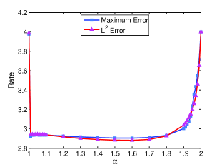
(a) $(p,q)=(1,0)$

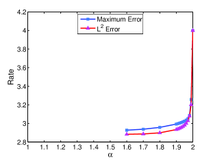
(b) $(p,q)=(1,-1)$

Figure 1: The convergence rates of the maximum and $L^{2}$ errors to 5.1 approximated by the compact difference scheme at $t=1$ with $N=128$.

Example 2.

The following fractional diffusion problem

$$\frac{\partial u(x,y,t)}{\partial t}={{}_{0}}D_{x}^{\alpha}u(x,y,t)+{{}_{x}}D_{1}^{\alpha}u(x,y,t)+{{}_{0}}D_{y}^{\beta}u(x,y,t)+{{}_{y}}D_{1}^{\beta}u(x,y,t)+f(x,y,t)$$ (5.2)

is considered in the domain $\Omega=(0,1)^{2}$ and $t>0$ with the boundary conditions

$$u(x,y,t)=0,\quad(x,y)\in\partial\Omega,\quad t\in[0,1],$$

and initial value

$$u(x,y,0)=u(x,y,0)=x^{3}(1-x)^{3}y^{3}(1-y)^{3},\quad(x,y)\in[0,1]^{2}.$$

The source term is

$$\begin{split}f(x,y,t)=-\mathrm{e}^{-t}\Big{[}&x^{3}(1-x)^{3}y^{3}(1-y)^{3}\\ &+\Big{(}\frac{\Gamma(4)}{\Gamma(4-\alpha)}\big{(}x^{3-\alpha}+(1-x)^{3-\alpha}\big{)}-\frac{3\Gamma(5)}{\Gamma(5-\alpha)}\big{(}x^{4-\alpha}+(1-x)^{4-\alpha}\big{)}\\ &+\frac{3\Gamma(6)}{\Gamma(6-\alpha)}\big{(}x^{5-\alpha}+(1-x)^{5-\alpha}\big{)}-\frac{\Gamma(7)}{\Gamma(7-\alpha)}\big{(}x^{6-\alpha}+(1-x)^{6-\alpha}\big{)}\Big{)}y^{3}(1-y)^{3}\\ &+\Big{(}\frac{\Gamma(4)}{\Gamma(4-\beta)}\big{(}y^{3-\beta}+(1-y)^{3-\beta}\big{)}-\frac{3\Gamma(5)}{\Gamma(5-\beta)}\big{(}y^{4-\beta}+(1-y)^{4-\beta}\big{)}\\ &+\frac{3\Gamma(6)}{\Gamma(6-\beta)}\big{(}y^{5-\beta}+(1-y)^{5-\beta}\big{)}-\frac{\Gamma(7)}{\Gamma(7-\beta)}\big{(}y^{6-\beta}+(1-y)^{6-\beta}\big{)}\Big{)}x^{3}(1-x)^{3}\Big{]}.\end{split}$$

And the exact solution of 5.1 is given by $u(x,t)=\mathrm{e}^{-t}x^{3}(1-x)^{3}y^{3}(1-y)^{3}$.

Table 2: The maximum and $L^{2}$ errors and corresponding convergence rates to 5.1 approximated by the compact difference splitting schemes at $t=1$ with $\tau=h$.

		$(p,q)=(1,0),(\alpha,\beta)=(1.1,1.7)$				$(p,q)=(1,-1),(\alpha,\beta)=(1.6,1.9)$
Scheme	$N$	$\|u^{n}-W^{n}\|_{\infty}$	rate	$\|u^{n}-W^{n}\|$	rate	$\|u^{n}-W^{n}\|_{\infty}$	rate	$\|u^{n}-W^{n}\|$	rate
	8	5.18337E-07	-	2.35962E-07	-	1.27051E-05	-	5.20284E-06	-
	16	7.47852E-08	2.79	3.12736E-08	2.92	8.45409E-07	3.91	3.09460E-07	4.07
	32	9.61857E-09	2.96	4.13976E-09	2.92	8.71092E-08	3.28	2.87346E-008	3.43
CLOD	64	1.28508E-09	2.90	5.56504E-10	2.90	9.67026E-09	3.17	3.35453E-009	3.10
	128	1.71211E-10	2.91	7.47594E-11	2.90	1.17863E-09	3.04	4.22753E-010	2.99
	256	2.26863E-11	2.92	9.97266E-12	2.91	1.49079E-10	2.98	5.43715E-011	2.96
	8	6.30467E-007	-	2.63036E-007	-	3.59941E-006	-	1.33801E-006	-
	16	7.67884E-008	3.04	3.20134E-008	3.04	5.12851E-007	2.81	1.88287E-007	2.83
	32	9.54417E-009	3.01	4.19273E-009	2.93	7.24724E-008	2.82	2.48958E-008	2.92
CPR	64	1.28241E-009	2.90	5.60865E-010	2.90	9.12654E-009	2.99	3.25063E-009	2.94
	128	1.71042E-010	2.91	7.51181E-011	2.90	1.15503E-009	2.98	4.22913E-010	2.94
	256	2.26759E-011	2.92	1.00029E-011	2.91	1.49068E-010	2.95	5.48530E-011	2.95
	8	6.28561E-007	-	2.54619E-007	-	3.01132E-006	-	1.15694E-006	-
	16	7.67367E-008	3.03	3.12227E-008	3.03	4.37299E-007	2.78	1.67892E-007	2.78
	32	9.54020E-009	3.01	4.12678E-009	2.92	6.67372E-008	2.71	2.30759E-008	2.86
CDouglas	64	1.28220E-009	2.90	5.55710E-010	2.89	8.61113E-009	2.95	3.09798E-009	2.90
	128	1.71028E-010	2.91	7.47144E-011	2.89	1.11175E-009	2.95	4.09795E-010	2.92
	256	2.26748E-011	2.92	9.97005E-012	2.91	1.45187E-010	2.94	5.36563E-011	2.93
	8	6.28561E-007	-	2.54619E-007	-	3.01132E-006	-	1.15694E-006	-
	16	7.67367E-008	3.03	3.12227E-008	3.03	4.37299E-007	2.78	1.67892E-007	2.78
	32	9.54020E-009	3.01	4.12678E-009	2.92	6.67372E-008	2.71	2.30759E-008	2.86
CD’yakonov	64	1.28220E-009	2.90	5.55710E-010	2.89	8.61113E-009	2.95	3.09798E-009	2.90
	128	1.71028E-010	2.91	7.47144E-011	2.89	1.11175E-009	2.95	4.09795E-010	2.92
	256	2.26748E-011	2.92	9.97005E-012	2.91	1.45187E-010	2.94	5.36563E-011	2.93

In Table 2, the errors $\|u^{n}-W^{n}\|,\|u^{n}-W^{n}\|_{\infty}$ and their respective convergence rates are presented for different uniformly space stepsizes, where $W_{i,j}^{n}(\tau)=-\frac{1}{3}U_{i,j}^{n}(\tau)+\frac{4}{3}U_{i,j}^{n}(\tau/2)$ is the numerical solution by extrapolation in time, and $U_{i,j}^{n}$ satisfies the compact LOD scheme 4.18, compact Peaceman-Richardson scheme 4.11, compact Douglas scheme 4.12 and compact D’yakonov scheme 4.13, respectively. The third order accuracy both in time and space is verified, and in the computational process, the time costs are largely reduced.

6 Conclusion

In [24], we introduce the weighted and shifted Grünwald difference (WSGD) operators and show that the WSGD operators have second order accuracy to approximate the fractional derivatives. This paper is the sequel of [24]. Based on the WSGD operators, we further introduce the compact WSGD operators (CWSGD) which have third order accuracy. Then we use the CWSGD operators to establish the compact difference schemes for one and two dimensional space fractional diffusion equations. And the theoretical analysis of the stability and convergence of the schemes is presented. The numerical results illustrate the effectiveness of the compact difference approximation for the fractional problems and confirm the convergence orders of the schemes.

7 Acknowledgements

The authors thank Prof Yujiang Wu for his constant encouragement and support. This work was supported by the Program for New Century Excellent Talents in University under Grant No. NCET-09-0438, the National Natural Science Foundation of China under Grant No. 10801067, and the Fundamental Research Funds for the Central Universities under Grant No. lzujbky-2010-63 and No. lzujbky-2012-k26.

References

- [1] E. Barkai, CTRW pathways to the fractional diffusion equation, Chem. Phys. 284 (2002) 13-27
- [2] D. A. Benson, S. W. Wheatcraft, M. M. Meerschaert, Application of a fractional advection-dispersion equation, Water Resour. Res. 36 (2000) 1403-1412
- [3] A. S. Chaves, A fractional diffusion equation to describe Lévy flights, Phys. Lett. A. 239 (1998) 13-16
- [4] R. Gorenflo, F. Mainardi, Random walk models for space-fractional diffusion processes, Fract. Calc. Appl. Anal. 1 (1998) 167-191
- [5] A. J. Laub, Matrix Analysis for Scientists and Engineers, SIAM (2005)
- [6] R. J. Leveque, Finite Difference Methods for Ordinary and Partial Differential Equations, SIAM (2007)
- [7] H. L. Liao, Z. Z. Sun, Maximum norm error bounds of ADI and compact ADI methods for solving parabolic equations, Numer. Methods Partial Differential Equations. 26 (2008) 37-60
- [8] C. Li, W. H. Deng, Y. J. Wu, Finite difference approximations and dynamics simulations for the L vy Fractional Klein-Kramers equation, Numer. Methods Partial Differential Equations. DOI: 10.1002/num.20709
- [9] G. I. Marchuk, V. V. Shaidurov, Difference Methods and Their Extrapolations, Springer-Verlag, New York, 1983
- [10] R. Metzler, J. Klafter, The random walk’s guide to anomalous diffusion: A fractional dynamics approach, Phys. Rep. 339 (2000) 1-77
- [11] R. Metzler, J. Klafter, The restaurant at the end of the random walk: recent developments in the description of anomalous transport by fractional dynamics, J. Phys. A: Math. Gen. 37 (2004) R161 CR208
- [12] M. M. Meerschaert, C. Tadjeran, Finite difference approximations for fractional advection-dispersion flow equations, J. Comput. Appl. Math. 172 (2004) 65-77
- [13] M. M. Meerschaert, C. Tadjeran, Finite difference approximations for two-sided space-fractional partial differential equations, Appl. Numer. Math. 56 (2006) 80-90
- [14] M. M. Meerschaert, H. P. Scheffler, C. Tadjeran, Finite difference methods for two-dimensional fractional dispersion equation, J. Comput. Phys. 211 (2006) 249-261
- [15] I. Podlubny, Fractional Differential Equations, Academic Press, San Diego (1999)
- [16] M. Marcus, H. Minc, A Survey of Matrix Theory and Matrix Inequalities, Allyn & Bacon. Inc (1964)
- [17] J. Qin, T. Wang, A compact locally one-dimensional finite difference method for nonhomogeneous parabolic differential equations, Int. J. Numer. Meth. Biomed. Engng. 27 (2011) 128-142
- [18] A. Quarteroni, A. Valli, Numerical Approximation of Partial Differential Equations, Springer (1997)
- [19] E. Scalas, R. Gorenflo, F. Mainardi, Fractional calculus and continuous-time finance, Phys. A. 284 (2000) 376-384
- [20] T. K. Sengupta, G. Ganerwal, A. Dipankar, High accuracy compact schemes and Gibb’s pheonomenon, J. Sci. Comput. 21 (2004) 253-268
- [21] C. Tadjeran, M. M. Meerschaert, H. P. Scheffler, A second-order accurate numerical approximation for the fractional diffusion equation, J. Comput. Phys. 213 (2006) 205-213
- [22] C. Tadjeran, M. M. Meerschaert, A second-order accurate numerical approximation for the two-dimensional fractional diffusion equation, J. Comput. Phys. 220 (2007) 813-823
- [23] Z. F. Tian, Y. B. Ge, A fourth-order compact ADI method for solving two-dimensional unsteady convection-diffusion problems, J. Comput. Appl. Math. 198 (2007) 268-286
- [24] W. Y. Tian, H. Zhou, W. H. Deng, A class of second order difference approximation for solving space fractional diffusion equations, submitted. arXiv:1201.5949 [math.NA]
- [25] G. M. Zaslavsky, Chaos, fractional kinetic, and anomalous transport, Phys. Rep. 371 (2002) 461-580
- [26] F. Z. Zhang, Matrix Theory: Basic Results and Techniques, 2nd ed., Springer (2011)