Noise, Bifurcations, and Modeling of Interacting Particle Systems

Abstract

We consider the stochastic patterns of a system of communicating, or coupled, self-propelled particles in the presence of noise and communication time delay. For sufficiently large environmental noise, there exists a transition between a translating state and a rotating state with stationary center of mass. Time delayed communication creates a bifurcation pattern dependent on the coupling amplitude between particles. Using a mean field model in the large number limit, we show how the complete bifurcation unfolds in the presence of communication delay and coupling amplitude. Relative to the center of mass, the patterns can then be described as transitions between translation, rotation about a stationary point, or a rotating swarm, where the center of mass undergoes a Hopf bifurcation from steady state to a limit cycle. Examples of some of the stochastic patterns will be given for large numbers of particles.

I INTRODUCTION

The collective motion of interacting multi-particle systems has been the subject of many recent experimental and modeling studies. It is especially astounding that numerous coherent states of great complexity can arise spontaneously in spite of the absence of a particle acting as a leader. The study of these swarming systems has proven useful in understanding the spatio-temporal patterns formed by bacterial colonies, fish, birds, locusts, ants, pedestrians, etc. [1, 2, 3, 4, 5, 6]. Moreover, these studies have provided valuable information that may be exploited in the design of systems of autonomous, inter-communicating robotic systems [7, 8, 9].

Investigators have used various mathematical approaches to study swarm systems. Some studies have preserved the individual character of each agent in the system, using ordinary or delay differential equations (ODEs/DDEs) to describe their trajectories [10, 11, 12, 8]. Other researchers have proposed continuum models written in terms of averaged velocity and particle density fields that satisfy partial differential equations (PDEs) [2, 3, 5, 6]. In addition, authors have also studied the effects of noise in the swarms and shown the existence of noise-induced transitions [13, 14].

More recently, authors have begun to study the effects of communication time-delays between particles. Time-delay models are common in many areas of mathematical biology including population dynamics, neural networks, blood cell maturation, virus dynamics and genetic networks [15, 16, 17, 18, 19, 20, 21, 22, 23]. In the context of swarming particles, it has been shown that the introduction of a communication time-delay may induce transitions between different coherent states [14]. The type of transition is dependent on the coupling strength between particles and the noise intensity.

Here we make a more detailed study of the bifurcation structure of the mean field approximation to the delay-coupled model proposed studied in [14] and investigate how the bifurcations in the system are modified in the presence of noise.

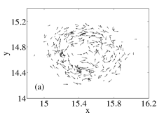
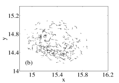
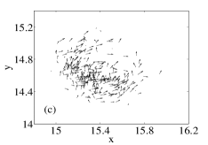
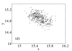
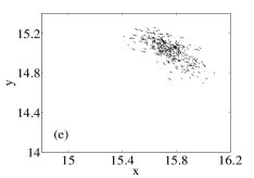
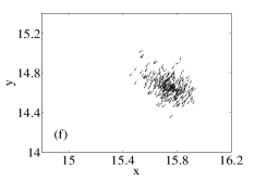
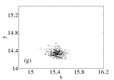
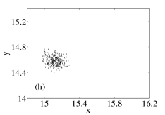
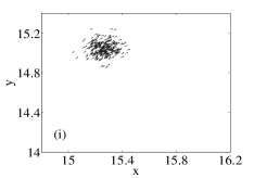
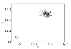
Figure 1: Snapshots of a swarm taken at (a) $t=50$, (b) $t=60$, (c) $t=62$, (d) $t=64$, (e) $t=66$, (f) $t=68$, (g) $t=70$, (h) $t=72$, (i) $t=74$, and (j) $t=76$, with $a=4$, $N=300$, and $D=0.08$. The swarm was in a rotational state when the time delay of $\tau=1$ was switched on at $t=40$. For a movie, see the relevant mpeg video. Figure reproduced with permission from [14].

II The Swarm Model

We consider a two-dimensional swarm with $N$ self-propelling particles that are mutually attracted in a symmetric fashion. Additionally, we consider the case in which particles communicate with each other with a time delay. The swarm is governed by the following system of ODEs:

$$\dot{\mathbf{r}}_{i}= \mathbf{v}_{i},$$ (1a)

$$\dot{\mathbf{v}}_{i}= \left(1-|\mathbf{v}_{i}|^{2}\right)\mathbf{v}_{i}-\frac{a}{N}\mathop{\sum_{j=1}^{N}}_{i\neq j}(\mathbf{r}_{i}(t)-\mathbf{r}_{j}(t-\tau))+\boldsymbol{\eta}_{i}(t),$$ (1b)

for $i=1,2\ldots,N$. Here $\mathbf{r}_{i}$ and $\mathbf{v}_{i}$ represent the position and velocity of the $i$-th particle, respectively; the strength of the attraction is measured by the coupling constant $a$ and the time delay is uniform and given by $\tau$. The self- propulsion and frictional drag on each particle is given by the term $\left(1-|\mathbf{v}_{i}|^{2}\right)\mathbf{v}_{i}$. In the absence of coupling, particles tend to move on a straight line with unit speed $|\mathbf{v}_{i}|=1$ as time goes to infinity. The term $\boldsymbol{\eta}_{i}(t)=(\eta_{i}^{(1)},\eta_{i}^{(2)})$ is a two-dimensional vector of stochastic white noise with intensity equal to $D$ and correlation functions $\langle\eta_{i}^{(\ell)}(t)\rangle=0$ and $\langle\eta_{i}^{(\ell)}(t)\eta_{j}^{(k)}(t^{\prime})\rangle=2D\delta(t-t^{\prime})\delta_{ij}\delta_{\ell k}$ for $i,j=1,2,\ldots N$ and $\ell,k=1,2$.

The coupling between particles arises from a time-delayed, spring-like potential. Hence, our equations of motion may be considered to be the first term in a Taylor expansion of other more general time-delayed potential functions about an equilibrium point. The model described by Eqs. (1a)-(1b) with $\tau=0$ (i.e. no time delay) possesses a noise-induced transition whereby a large enough noise intensity causes a translating swarm of individuals to transition to a rotating swarm with a stationary center of mass [24, 14]. Regardless of which state the swarm is in (translating or rotating), the addition of a communication time delay leads to another type of transition. This transition occurs if the coupling parameter $a$, is large enough. As an example, we consider a swarm that has already undergone a noise-induced transition to a rotational state before switching on the communication time delay.

Figures 1(a)-1(j) show snapshots of a swarm at $t=50$, $t=60$, $t=62$, $t=64$, $t=66$, $t=68$, $t=70$, $t=72$, $t=74$, and $t=76$ respectively. For these simulations, $N=300$, $\tau=1$, $D=0.08$, the noise was switched on at $t=10$ (causing the swarm to transition to a stationary, rotating state), and once in this rotating state, the time delay was switched on at $t=40$. One can see that with the evolution of time, the individual particles become aligned with one another and the swarm becomes more compact. Additionally, the swarm is no longer stationary, but has begun to oscillate [Figs. 1(g)-1(j)].

This compact, oscillating aligned swarm state looks similar to a single “clump” that is described in [25]. However, where each “clump” of [25] contains only some of the total number of swarming particles, our swarm contains every particle. Additionally, while a deterministic model along with global coupling is used to attain the “clumps” of [25], our oscillating aligned swarm is attained with the use of noise and a time delay.

III Mean Field Approximation

As we have shown, once the stochastic swarm is in the stationary, rotating state, the addition of a time delay induces an instability. We investigate the stability of the swarm by deriving the mean field equations and performing a bifurcation analysis.

We carry out a mean field approximation of the swarming system by switching to particle coordinates relative to the center of mass and disregarding the noise terms. The center of mass of the swarming system is given by

$$\mathbf{R}(t)=\frac{1}{N}\sum_{i=1}^{N}\mathbf{r}_{i}(t).$$ (2)

We decompose the position of each particle into

$$\mathbf{r}_{i}=\mathbf{R}+\delta\mathbf{r}_{i},\qquad i=1,2\ldots,N,$$ (3)

where

$$\sum_{i=1}^{N}\delta\mathbf{r}_{i}(t)=0.$$ (4)

Inserting Eq. (3) into the second order system equivalent to Eqs. (1a)-(1b) with $D=0$ and simplifying one obtains

$$\ddot{\mathbf{R}}+\delta\ddot{\mathbf{r}}_{i}= \left(1-|\dot{\mathbf{R}}|^{2}-2\dot{\mathbf{R}}\cdot\delta\dot{\mathbf{r}}_{i}-|\delta\dot{\mathbf{r}}_{i}|^{2}\right)(\dot{\mathbf{R}}+\delta\dot{\mathbf{r}_{i}})$$

$$-\frac{a(N-1)}{N}\bigg{(}\mathbf{R}(t)-\mathbf{R}(t-\tau)+\delta\mathbf{r}_{i}(t)\bigg{)}$$

$$-\frac{a}{N}\delta\mathbf{r}_{i}(t-\tau),$$ (5)

where we used Eq. (4) in the form

$$\delta\mathbf{r}_{i}(t-\tau)=-\sum_{j=1,\ i\neq j}^{N}\delta\mathbf{r}_{j}(t-\tau).$$ (6)

Summing Eq. (III) over $i$ and using Eq. (4), one arrives at

$$\ddot{\mathbf{R}}= \left(1-|\dot{\mathbf{R}}|^{2}-\frac{1}{N}\sum_{i=1}^{N}|\delta\dot{\mathbf{r}}_{i}|^{2}\right)\dot{\mathbf{R}}$$

$$-\frac{1}{N}\sum_{i=1}^{N}\left(2\dot{\mathbf{R}}\cdot\delta\dot{\mathbf{r}}_{i}+|\delta\dot{\mathbf{r}}_{i}|^{2}\right)\delta\dot{\mathbf{r}_{i}}$$

$$-a\frac{N-1}{N}\left(\mathbf{R}(t)-\mathbf{R}(t-\tau)\right).$$ (7)

Inserting Eq. (III) into Eq. (III) the following equation for $\delta\ddot{\mathbf{r}}_{i}$ is obtained:

$$\delta\ddot{\mathbf{r}}_{i}= \left(\frac{1}{N}\sum_{j=1}^{N}|\delta\dot{\mathbf{r}}_{j}|^{2}-2\dot{\mathbf{R}}\cdot\delta\dot{\mathbf{r}}_{i}-|\delta\dot{\mathbf{r}}_{i}|^{2}\right)\dot{\mathbf{R}}$$

$$+\left(1-|\dot{\mathbf{R}}|^{2}-2\dot{\mathbf{R}}\cdot\delta\dot{\mathbf{r}}_{i}-|\delta\dot{\mathbf{r}}_{i}|^{2}\right)\delta\dot{\mathbf{r}}_{i}$$

$$+\frac{1}{N}\sum_{j=1}^{N}\left(2\dot{\mathbf{R}}\cdot\delta\dot{\mathbf{r}}_{j}+|\delta\dot{\mathbf{r}}_{j}|^{2}\right)\ \delta\dot{\mathbf{r}}_{j}-a\frac{N-1}{N}\delta\mathbf{r}_{i}$$

$$-\frac{a}{N}\delta\mathbf{r}_{i}(t-\tau),$$ (8)

for $i=1,2\ldots,N$.

Equations (III) and (III) are fully equivalent to Eqs. (1a)-(1b) when $D=0$, and simply consist of rewriting the original system using the relationship between the particle coordinates $\mathbf{r}_{i}$, the center of mass $\mathbf{R}$, and the coordinates relative to the center of mass $\delta\mathbf{r}_{i}$. This mapping has transformed the original $2N$ differential equations into $2N+2$ differential equations. There is, however, no inconsistency since in the transformed set of equations only $2N$ of them are independent, because of the relation seen in Eq. (4).

We then obtain a mean field approximation by neglecting the fluctuation of the swarm particles, $\delta\mathbf{r}_{i}$’s, from the center of mass:

$$\ddot{\mathbf{R}}= \left(1-|\dot{\mathbf{R}}|^{2}\right)\dot{\mathbf{R}}-a\left(\mathbf{R}(t)-\mathbf{R}(t-\tau)\right),$$ (9)

where we made the approximation $a\frac{N-1}{N}\approx a$ since we consider the thermodynamic limit.

IV Bifurcations in the Mean Field Equation

The behavior of the system in the mean field approximation in different regions of parameter space may be better understood by using bifurcation analysis. Equation (9) may be written in component form using $\mathbf{R}=(X,Y)$ and $\dot{\mathbf{R}}=(U,V)$ as

$$\dot{X} =U,$$ (10a)

$$\dot{U} =(1-U^{2}-V^{2})U-a(X-X(t-\tau)),$$ (10b)

$$\dot{Y} =V,$$ (10c)

$$\dot{V} =(1-U^{2}-V^{2})V-a(Y-Y(t-\tau)).$$ (10d)

For all values of $a$ and $\tau$, Eqs. (10a)-(10d) have translationally invariant stationary solutions

$$X=X_{0},\quad U=0,\quad Y=Y_{0},\quad V=0,$$ (11)

with two free parameters $X_{0}$ and $Y_{0}$. They also have a three parameter family of uniformly translating solutions

$$X=U_{0}t+X_{0},\quad U=U_{0},\quad Y=V_{0}t+Y_{0},\quad V=V_{0},$$ (12)

which requires

$$U_{0}^{2}+V_{0}^{2}=1-a\tau,$$ (13)

and thus exists only for $a\tau<1$. In the two-parameter space $(a,\tau)$, the hyperbola $a\tau=1$ is in fact a pitchfork bifurcation line on which the uniformly translating states are born from the stationary state $(X_{0},0,Y_{0},0)$. The other branch of the pitchfork is an unphysical solution with negative speed.

Linearizing Eqs. (10a)-(10d) about the stationary state, we obtain the characteristic equation

$$\left(a(1-e^{-\lambda\tau})-\lambda+\lambda^{2}\right)^{2}=0.$$ (14)

It suffices to study the zeros of the function

$${\cal{D}}(\lambda)=a(1-e^{-\lambda\tau})-\lambda+\lambda^{2}=0,$$ (15)

since the eigenvalues of Eqs. (10a)-(10d) are obtained by duplicating those of Eq. (15).

We now search for Hopf bifurcations in the two parameter space $(a,\tau)$ by letting $\lambda=i\omega$ in Eq. (15). Substitution leads to

$$a-\omega^{2}-i\omega=ae^{-i\omega\tau}.$$ (16)

Taking the modulus of Eq. (16), we find $a$ at the Hopf point, $a_{H}$, is given by

$$a_{H}^{2}=(a_{H}-\omega^{2})^{2}+\omega^{2},$$ (17)

or, considering $\omega\neq 0$,

$$a_{H}=\frac{1+\omega^{2}}{2}.$$ (18)

We eliminate $a$ in Eq. (16) by using Eq. (18) and taking the complex conjugate to obtain an equation for $\tau$ at the Hopf point

$$\frac{1-\omega^{2}}{1+\omega^{2}}+i\frac{2\omega}{1+\omega^{2}}=e^{i\omega\tau}.$$ (19)

We obtain $\tau$ by equating the arguments of both sides, being careful to use the branch of $\tan\theta$ in $(0,\pi)$ since the left hand side of Eq. (19) is on the upper complex plane for $\omega>0$. The result is a family of Hopf bifurcation curves parameterized by $\omega$:

$$a_{H}(\omega) =\frac{1+\omega^{2}}{2},$$ (20a)

$$\tau_{Hn}(\omega) =\frac{1}{\omega}\left(\arctan\left(\frac{2\omega}{1-\omega^{2}}\right)+2n\pi\right)$$

$$n =0,1,\ldots.$$ (20b)

These curves are shown in Fig. 2. We may eliminate the parameter $\omega$ between these two equations and obtain

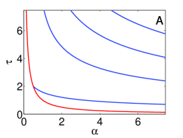
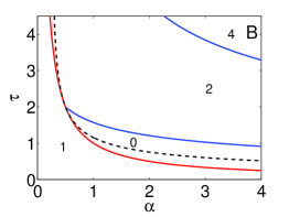
Figure 2: (a) Hopf (blue) and pitchfork (red) bifurcation curves in $a$ and $\tau$ space. (b) A zoom-in of the branches in the first panel displaying also the saddle to node transition (dashed black); the number in each region indicates the number of eigenvalues with a real part greater than zero with the solid lines as boundaries. (Color online.)

$$\tau_{Hn}(a) =\frac{1}{\sqrt{2a-1}}\left(\arctan\left(\frac{\sqrt{2a-1}}{1-a}\right)+2n\pi\right)$$

$$n =0,1,\ldots$$ (21)

In spite of their appearance, the Hopf curves in Eqs. (20a)-(20) and (IV) are in fact continuous at $\omega=1$ and $a=1$, respectively (with the correct branch of $\tan\theta$ in $(0,\pi)$). From Eq. (20a)-(20), we see that the Hopf frequency depends only on the value of $a$ for all members in the family; it has the value one at $a=1$ and the frequency tends to infinity as $a$ grows. Interestingly, only the first Hopf curve of the family in Eq. (IV) is defined at $a=1/2$; it has the value $\tau_{H0}|_{a=1/2}=2$. The point ($a=1/2$, $\tau=2$) which lies both on the first member of the family of Hopf curves and on the pitchfork branch is in fact a Bogdanov-Takens (BT) point [26], where $\omega=0$. None of the other Hopf branches meet the pitchfork bifurcation line since they tend asymptotically to infinity as $a\rightarrow 1/2$.

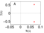
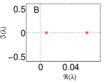
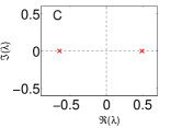
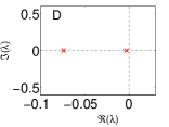
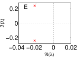
Figure 3: Location of the dominating eigenvalues around the Bogdanov-Takens point at $a=1/2$, $\tau=2$. Parameter values are (a) $a=0.60$, $\tau=2.0$, (b) $a=0.48$, $\tau=2.09$, (c) $a=0.40$, $\tau=2.01$, (d) $a=0.53$, $\tau=1.90$, and (e) $a=0.55$, $\tau=1.91$.

We used a numerical continuation method (DDE-Biftool) [27] to calculate the pitchfork and Hopf branches in the $(a,\tau)$ parameter space; these results are in perfect agreement with our analytical calculations (results not shown). These numerical studies reveal that the number of eigenvalues with real part greater than zero is as indicated in Fig. 2. In addition, our numerical continuation analyses also reveal node to focus transitions of the steady state. These occur at points where there are two real and equal eigenvalues, i.e. where ${\cal{D}}(\lambda)=0$ and ${\cal{D}^{\prime}}(\lambda)=0$, for $\lambda$ real. From ${\cal{D}^{\prime}}(\lambda)=0$ we obtain $e^{-\tau\lambda}=\frac{1-2\lambda}{a\tau}$, which we can insert into ${\cal{D}}(\lambda)=0$ to obtain

$$\lambda^{2}-\left(1-\frac{2}{\tau}\right)\lambda+a-\frac{1}{\tau}=0,$$ (22)

with solutions $\lambda=\frac{1}{2}\left[1-\frac{2}{\tau}\pm\sqrt{1+\frac{4}{\tau^{2}}-4a}\right]$. For the roots to be repeated, we set the discriminant to zero and this gives the curve where the node-focus transitions occur:

$$\tau=\frac{1}{\sqrt{a-1/4}}.$$ (23)

Moreover, from the solutions to Eq. (22) we see that the repeated eigenvalues have positive real parts if $\tau>2$ and negative real parts if $\tau<2$. In Fig. 2, we show the pitchfork and Hopf bifurcation curves overlaid with the node-focus transition curve given by Eq. (23).

As seen in Fig. 2, the pitchfork and Hopf branches, together with the node-focus transition curves split the area around the BT point into five different regions. The behavior of the leading eigenvalues (excluding the one at the origin) as one probes these five regions is shown in Figs. 3-3. At a point directly to the right of the BT point in $(a,\tau)$ space, the stationary solution has a pair of eigenvalues with positive real parts and non-zero imaginary parts [Fig. 3]. Moving counter-clockwise in the $(a,\tau)$ plane, the eigenvalue pair collapses onto the real line after crossing the upper branch of the node-focus transition [Fig. 3]. Still moving in the same direction in parameter space, we observe two different instances of eigenvalues crossing the origin: first, the smaller of the two purely real and positive eigenvalues does so on the upper part of the pitchfork bifurcation line [Fig. 3] and then the remaining purely real and positive eigenvalue crosses the origin on the lower part of the bifurcation line [Fig. 3]. Finally, at the node-focus transition line, the two purely real and negative eigenvalues coincide on the real axis and acquire non-zero imaginary parts [Fig. 3]. Continuing upwards in parameter space, the complex pair crosses the imaginary axis on the Hopf bifurcation curve, giving birth to a stable limit cycle.

IV-A Numerical simulations

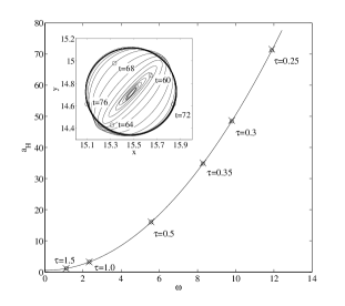
Figure 4: The limit cycle of the center of mass is shown through a comparison of analytical (solid line) and numerical (“cross” markers) values of $a_{H}$ and $\omega$ for several choices of $\tau$. The analytical result is found using Eqs. (20a)-(20), while the numerical result is found using a continuation method [27] for Eq. (9). The inset shows the stochastic trajectory of the center of mass of the swarm from $t=45$ to $t=90$.Figure reproduced with permission from [14].

Figure 4 shows an excellent comparison of the analytical result given by Eqs. (20a)-(20) with a numerical result which was found using a continuation method [27] for the mean field model for several choices of $\tau$. Furthermore, for $\tau=1$, the value of coupling $a$ at the bifurcation point is $a_{H}\approx 3.2$. This value of $a_{H}$ corresponds very well to the change in behavior of the stochastic swarm (results not shown).

More evidence of the Hopf bifurcation is seen in the inset of Fig. 4. The inset shows the stochastic trajectory of the center of mass of the swarm from $t=45$ to $t=90$ for the example shown in Fig. 1. Once the time delay is switched on at $t=40$ (with the swarm located at the center of the inset figure), the swarm begins to oscillate. The swarm moves along an elliptical path [the position of its center of mass is denoted at several times that correspond to Figs. 1(b), 1(d), 1(f), 1(h), and 1(j)], until it eventually converges to the circular limit cycle.

Figures 5 and 5 show a time series simulation of a swarm with $N=75$ particles. Figure 5 shows the position components, while Fig. 5 shows the velocity components., One can see that the swarm follows a circular-like path over time. A perturbation that is applied at $t=20$ shows that for the chosen parameters, the pattern is stable in the presence of noise.

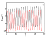
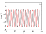
Figure 5: The limit cycle of the center of mass is shown through the (a) position and (b) velocity time series of the swarm using $N=75$ particles, $a=0.7$, $\tau=2.2$, and noise intensity $D=0.045$. A velocity perturbation is applied at $t=20$.

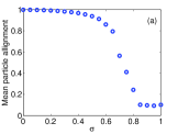
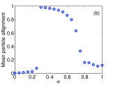
Figure 6: Long time behavior of the mean particle alignment (defined in the text) for different values of noise intensity ($D=\sigma^{2}/2$) and two different initial conditions. In panel (a), all particles start off from the origin with equal velocity vectors; in panel (b), all particles start from rest, distributed uniformly over the unit square. For these simulations, $N=150$, $a=2$ and $\tau=2$. The time-delay is turned on at $t=50$, and the simulations run until $t=300$.

The presence of noise introduces interesting switching behavior that make the initial conditions of the swarm critical in determining the long time behavior of the system. To demonstrate this, we have performed a series of simulations for different noise intensities and two different initial conditions: (i) all particles start at the origin with unit $x$ and $y$ speeds [Fig. 6] and (ii) all particles are distributed uniformly over the unit square and start from rest [Fig. 6]. The simulations are run until $t=300$ using a coupling constant $a=2$ and a time-delay $\tau=2$ which is turned on at $t=50$. Our simulations reveal that in the long time limit and for small values of noise, the swarm converges to either a compact state that rotates as a whole [case (i)] or to a ring state with particles going both clockwise and counterclockwise [case (ii)]. The asymptotic behavior of the system is readily visualized by calculating the mean alignment of the swarm particles. We quantify this mean alignment of the swarm by calculating the cosine between the directions of the $i$-th particle and the center of mass, $\cos\theta_{i}=(\dot{\mathbf{r}}_{i}\cdot\dot{\mathbf{R}})/(|\dot{\mathbf{r}}_{i}||\dot{\mathbf{R}}|)$, and then averaging over all particles and over the last 100 time units of simulation. Figure 6 shows that in case (i) the particles converge to the compact, aligned state for low and moderate noise intensities. However, this state is broken up at high noise levels ($\sigma\approx 0.8$). In contrast, Fig. 6 shows that in case (ii) the particles converge to a ring for small values of noise ($\sigma\lesssim 0.25$), evidenced by the low values of the mean particle alignment in Fig. 6, but converge to the aligned case for higher values of noise ($\sigma\gtrsim 0.25$). Observing the full simulation runs in detail (not shown) reveals a switching behavior: for case (ii) with a noise level $\sigma\gtrsim 0.25$, the particles first converge to a noisy ring and then switch to the rotating state due to the effect of noise. The simulations suggest that the transition to the rotating state occurs once the velocities of the particles cross an alignment threshold. The system, in fact, displays hysteresis: one can force the swarm to transition from the ring state with $\sigma=0.2$ to the rotating state by raising the noise to $\sigma=0.25$; however, it seems that the inverse transition, i.e. making the swarm transition back to the ring state by lowering the noise level, is extremely unlikely.

V CONCLUSIONS

To summarize, we studied the dynamics of a self-propelling swarm in the presence of noise and a constant communication time delay and prove that the delay induces a transition that depends upon the size of the interaction coupling coefficient. Although our analytical and numerical results were obtained using a model with linear, attractive interactions, the analysis may be applied to models with more general forms of social interaction.

We further uncovered a complete analytical description of the bifurcation point which control the instabilities arising from noise induced transitions. The analysis allows us to completely classify, using mean field approximations, where the swarm exhibits a stable translation, stationary center of mass, or rotation.

In general, our results provide insight into the stability of complex systems comprised of individuals interacting with one another with a finite time delay in a noisy environment. Furthermore, the results may prove to be useful in controlling man-made vehicles where actuation and communication are delayed, as well as in understanding swarm alignment in biological systems.

VI ACKNOWLEDGMENTS

The authors gratefully acknowledge the Office of Naval Research for their support. LMR and IBS are supported by Award Number R01GM090204 from the National Institute Of General Medical Sciences. The content is solely the responsibility of the authors and does not necessarily represent the official views of the National Institute Of General Medical Sciences or the National Institutes of Health. E.F. is supported by the Naval Research Laboratory (Award No. N0017310-2-C007).

References

- [1] E. Budrene and H. Berg, “Dynamics of formation of symmetrical patterns by chemotactic bacteria,” Nature, vol. 376, no. 6535, pp. 49–53, 1995.
- [2] J. Toner and Y. Tu, “Long-range order in a two-dimensional dynamical xy model: How birds fly together,” Phys. Rev. Lett., vol. 75, no. 23, pp. 4326–4329, 1995.
- [3] ——, “Flocks, herds, and schools: A quantitative theory of flocking,” Phys. Rev. E, vol. 58, no. 4, pp. 4828–4858, 1998.
- [4] J. K. Parrish, “Complexity, pattern, and evolutionary trade-offs in animal aggregation,” Science, vol. 284, no. 5411, pp. 99–101, Apr 1999.
- [5] L. Edelstein-Keshet, J. Watmough, and D. Grunbaum, “Do travelling band solutions describe cohesive swarms? an investigation for migratory locusts,” J. Math. Biol., vol. 36, no. 6, pp. 515–549, 1998.
- [6] C. Topaz and A. Bertozzi, “Swarming patterns in a two-dimensional kinematic model for biological groups,” SIAM J. Appl. Math., vol. 65, no. 1, pp. 152–174, 2004.
- [7] N. Leonard and E. Fiorelli, “Virtual leaders, artificial potentials and coordinated control of groups,” Decision and Control, 2001. Proceedings of the 40th IEEE Conference on, vol. 3, pp. 2968–2973, 2002.
- [8] E. Justh and P. Krishnaprasad, “Steering laws and continuum models for planar formations,” Decision and Control, 2003. Proceedings. 42nd IEEE Conference on, vol. 4, pp. 3609–3614, 2004.
- [9] D. Morgan and I. Schwartz, “Dynamic coordinated control laws in multiple agent models,” Phys. Lett. A, vol. 340, no. 1-4, pp. 121–131, 2005.
- [10] T. Vicsek, A. Czirók, E. Ben-Jacob, I. Cohen, and O. Shochet, “Novel type of phase transition in a system of self-driven particles,” Phys. Rev. Lett., vol. 75, no. 6, pp. 1226–1229, 1995.
- [11] G. Flierl, D. Grünbaum, S. Levins, and D. Olson, “From individuals to aggregations: the interplay between behavior and physics,” J. Theor. Biol., vol. 196, no. 4, pp. 397–454, 1999.
- [12] I. Couzin, J. Krause, R. James, G. Ruxton, and N. Franks, “Collective memory and spatial sorting in animal groups,” J. Theor. Biol., vol. 218, no. 1, pp. 1–11, 2002.
- [13] U. Erdmann and W. Ebeling, “Noise-induced transition from translational to rotational motion of swarms,” Phys. Rev. E, vol. 71, 2005.
- [14] E. Forgoston and I. B. Schwartz, “Delay-induced instabilities in self-propelling swarms,” Phys. Rev. E, vol. 77, 035203(R), 2008.
- [15] N. MacDonald, Time Lags in Biological Models, 1st ed. Berlin: Springer-Verlag, 1978.
- [16] ——, Biological Delay Systems Models: Linear Stability Theory, 1st ed. Cambridge: Cambridge University Press, 1989.
- [17] I. Ncube, S. A. Campbell, and J. Wu, “Change in criticality of synchronous Hopf bifurcation in a multiple-delayed neural system,” Fields Inst. Commun., vol. 36, pp. 179–193, 2003.
- [18] S. Bernard, J. Bélair, and M. Mackey, “Bifurcations in a white-blood-cell production model,” C.R. Biol., vol. 327, pp. 201–210, 2004.
- [19] M. Mackey, M. Santillan, and N. Yildirim, “Modeling operon dynamics: The Tryptophan and lactose operons as paradigms,” C.R. Biol., vol. 327, pp. 211–224, 2004.
- [20] M. Mackey and M. Santillan, “Why is the lysogenic state of phage- is so stable: A mathematical modelling approach,” Biophys. J., vol. 86, pp. 75–84, 2004.
- [21] G. Tiana, M.H. Jensen, and K. Sneppen, “Time delay as a key to apoptosis in the p53 network,” Eur. Phys. J. B, vol. 29, pp. 135–140, 2002.
- [22] M.H. Jensen, K. Sneppen, and G. Tiana, “Sustained oscillations and time delays in gene expression of protein Hes1,” FEBS Lett., vol. 541, pp. 176–177, 2003.
- [23] N. Monk, “Oscillatory expression of Hes1, p53, and NF-B driven by transcriptional time delays,” Curr. Biol., vol. 13, pp. 1409–1413, 2003.
- [24] U. Erdmann, W. Ebeling, and A. S. Mikhailov, “Noise-induced transition from translational to rotational motion of swarms,” Phys. Rev. E, vol. 71, 051904, 2005.
- [25] M. R. D’Orsogna, Y. L. Chuang, A. L. Bertozzi, and L. S. Chayes, “Self-propelled particles with soft-core interactions: Patterns, stability, and collapse,” Phys. Rev. Lett., vol. 96, 104302, 2006.
- [26] J. Guckenheimer and P. Holmes, Nonlinear Oscillations, Dynamical Systems, and Bifurcations of Vector Fields, 2nd ed. Berlin: Springer-Verlag, 1983.
- [27] K. Engelborghs, “DDE-BIFTOOL: A Matlab package for bifurcation analysis of delay differential equations,” Department of Computer Science, K. U. Leuven, Belgium, Tech. Rep. TW-305, 2000. [Online. Available at: http://www.cs.kuleuven.ac.be/twr/research/software/delay/ddebiftool.shtml]