New bounds on the classical and quantum communication complexity of some graph properties

Abstract

We study the communication complexity of a number of graph properties where the edges of the graph $G$ are distributed between Alice and Bob (i.e., each receives some of the edges as input). Our main results are:

• An $\Omega(n)$ lower bound on the quantum communication complexity of deciding whether an $n$-vertex graph $G$ is connected, nearly matching the trivial classical upper bound of $O(n\log n)$ bits of communication.

• A deterministic upper bound of $O(n^{3/2}\log n)$ bits for deciding if a bipartite graph contains a perfect matching, and a quantum lower bound of $\Omega(n)$ for this problem.

• A $\Theta(n^{2})$ bound for the randomized communication complexity of deciding if a graph has an Eulerian tour, and a $\Theta(n^{3/2})$ bound for the quantum communication complexity of this problem.

The first two quantum lower bounds are obtained by exhibiting a reduction from the $n$-bit Inner Product problem to these graph problems, which solves an open question of Babai, Frankl and Simon [BFS86]. The third quantum lower bound comes from recent results about the quantum communication complexity of composed functions. We also obtain essentially tight bounds for the quantum communication complexity of a few other problems, such as deciding if $G$ is triangle-free, or if $G$ is bipartite, as well as computing the determinant of a distributed matrix.

1 Introduction

Graphs are among the most basic discrete structures, and deciding whether graphs have certain properties (being connected, containing a perfect matching, being 3-colorable, …) is among the most basic computational tasks. The complexity of such tasks has been studied in a number of different settings.

Much research has gone into the query complexity of graph properties, most of it focusing on the so-called Aandera-Karp-Rosenberg conjecture. Roughly speaking, this says that all monotone graph properties have query complexity $\Omega(n^{2})$. Here the vertex set is $[n]=\{1,\ldots,n\}$ and input graph $G=([n],E)$ is given as an adjacency matrix whose entries can be queried. This conjecture is proved for deterministic algorithms [RV76], but open for randomized ones [Haj91, CK07].

Less—but still substantial—effort has gone into the study of the communication complexity of graph properties [PS84, BFS86, HMT88, DP89]. Here the edges of $G$ are distributed over two parties, Alice and Bob. Alice receives set of edges $E_{A}$, Bob receives set $E_{B}$ (these sets may overlap), and the goal is to decide with minimal communication whether the graph $G=([n],E_{A}\cup E_{B})$ has a certain property.

In this paper we obtain new bounds for the communication complexity of a number of graph properties, both in the classical and the quantum world. Our main results are:

• An $\Omega(n)$ lower bound on the quantum communication complexity of deciding whether $G$ is connected, nearly matching the trivial classical upper bound of $O(n\log n)$ bits.

• Hajnal et al. [HMT88] state as an open problem to determine the communication complexity of deciding if a bipartite graph contains a perfect matching (i.e., a set of $n/2$ vertex-disjoint edges). We prove a deterministic upper bound of $O(n^{3/2}\log n)$ bits for this, and a quantum lower bound of $\Omega(n)$.

• For the problem of deciding if a graph contains an Eulerian tour we show that the quantum communication complexity is $\Theta(n^{3/2})$, whereas the randomized communication complexity is $\Theta(n^{2})$.

Our quantum lower bounds for the first two problems are proved by reductions from the hard inner product problem, which is $\mbox{\sc IP}_{n}(x,y)=\sum_{i=1}^{n}x_{i}y_{i}$ mod 2. Babai et al. [BFS86, Section 7] showed how to reduce the disjointness problem ($\mbox{\sc Disj}_{n}(x,y)=1$ iff $\sum_{i=1}^{n}x_{i}y_{i}=0$) to these graph problems, but left reductions from inner product as an open problem (they did reduce inner product to a number of other problems [BFS86, Section 9]). In the classical world this doesn’t make much difference since both Disj and IP require $\Omega(n)$ communication (the tight lower bound for Disj was proved only after [BFS86] in [KS92]). However, in the quantum world Disj is quadratically easier than IP, so reductions from IP give much stronger lower bounds in this case.

While investigating the communication complexity of graph properties is interesting in its own right, there have also been applications of lower bounds for such problems. For instance, communication complexity arguments have recently been used to show new and tight lower bounds for several graph problems in distributed computing in [DHK⁺11]. These problems include approximation and verification versions of classical graph problems like connectivity, $s$-$t$ connectivity, and bipartiteness. In their setting processors see only their local neighborhood in a network. [DHK⁺11] use reductions from Disj to establish their lower bounds. Subsequently some of these results have been generalized to the case of quantum distributed computing [EKNP12], employing for instance the new reductions from IP given in this paper, which in the quantum case establish larger lower bounds than the previous reductions from Disj.

2 Preliminaries

We assume familiarity with communication complexity, referring to [KN97] for more details about classical communication complexity and [Wol02] for quantum communication complexity (for information about the quantum model beyond what’s provided in [Wol02], see [NC00]).

Given some communication complexity problem $f:X\times Y\rightarrow R$ we use $D(f)$ to denote its classical deterministic communication complexity, $R_{2}(f)$ for its private-coin randomized communication complexity with error probability $\leq 1/3$, and $Q_{2}(f)$ for its private-coin quantum communication complexity with error $\leq 1/3$. Our upper bounds for the quantum model do not require prior shared entanglement; however, all lower bounds on $Q_{2}(f)$ in this paper also apply to the case of unlimited prior entanglement.

Among others we consider two well-known communication complexity problems, with $X=Y=\{0,1\}^{n}$ and $R=\{0,1\}$. For $x,y\in\{0,1\}^{n}$ we define $x\wedge y\in\{0,1\}^{n}$ as the bitwise AND of $x$ and $y$, and $|x|=|\{i\in[n]:x_{i}=1\}|$ as the Hamming weight of $x$.

• Inner product: $\mbox{\sc IP}_{n}(x,y)=|x\wedge y|$ mod 2. The quantum communication complexity of this problem is $Q_{2}(\mbox{\sc IP}_{n})=\Theta(n)$ [Kre95, CDNT98] (in fact even its unbounded-error quantum communication complexity is linear [For01]).

• Disjointness: $\mbox{\sc Disj}_{n}(x,y)=1$ if $|x\wedge y|=0$, and $\mbox{\sc Disj}_{n}(x,y)=0$ otherwise. Viewing $x$ and $y$ as the characteristic vectors of subsets of $[n]$, the task is to decide whether these sets are disjoint. It is known that $R_{2}(\mbox{\sc Disj}_{n})=\Theta(n)$ [KS92, Raz92] and $Q_{2}(\mbox{\sc Disj}_{n})=\Theta(\sqrt{n})$ [BCW98, AA05, Raz03]. In fact, the Aaronson-Ambainis protocol [AA05] can find an $i$ such that $x_{i}=y_{i}=1$ (if such an $i$ exists), using an expected number of $O(\sqrt{n})$ qubits of communication. This saves a log-factor compared to the more straightforward distributed implementation of Grover’s algorithm in [BCW98].

3 Reduction from Parity

We begin with a reduction from the $n$-bit Parity problem to the connectedness of a $2n$-vertex graph in the model of query complexity. This reduction was used by Dürr et al. [DHHM06, Section 8], who attribute it to Henzinger and Fredman [HF98]. The same reduction can be used to reduce Parity to determining if an $n$-by-$n$ bipartite graph contains a perfect matching. Our hardness results for communication complexity in later sections follow by means of simple gadgets to transfer this reduction from the query world to the communication world.

Claim 1.

For every $z\in\{0,1\}^{n}$ there is a graph $G_{z}$ with $2n$ vertices (where for each possible edge, its presence or absence just depends on one of the bits of $z$), such that if the parity of $z$ is odd then $G_{z}$ is a cycle of length $2n$, and if the parity of $z$ is even then $G_{z}$ is the disjoint union of two $n$-cycles.

Proof.

We construct a graph $G$ with $2n$ vertices, arranged in two rows of $n$ vertices each. We will label the vertices as $t_{i}$ and $b_{i}$ for $i\in[n]$ indicating if it is in the top row or the bottom row. For $i\in[n-1]$, if $z_{i}=0$ then add edges $\{t_{i},t_{i+1}\}$ and $\{b_{i},b_{i+1}\}$; if $z_{i}=1$ then add $\{t_{i},b_{i+1}\}$ and $\{b_{i},t_{i+1}\}$. For $i=n$ make the same connections with vertex $1$, wrapping around. See Figure 1 for illustration. If the parity of $z$ is odd then the resulting graph $G$ will be one $2n$-cycle, and if the parity is even then it will be two $n$-cycles. ∎

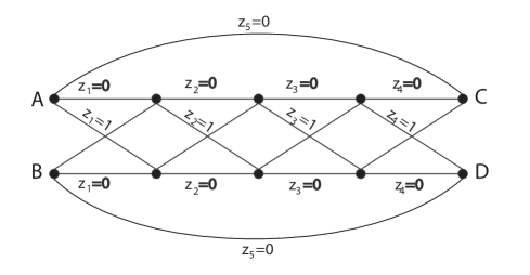
Figure 1: The string $z$ determines the edges present in $G_{z}$. If $z_{5}=1$ there are edges connecting A with D, and B with C (omitted for clarity). When the parity of $z$ is odd, the graph is a $2n$-cycle, and when it is even the graph is the disjoint union of two $n$-cycles.

4 Connectedness

We first focus on the communication complexity of deciding whether a graph $G$ is connected or not. Denote the corresponding Boolean function for $n$-vertex graphs by $\mbox{\sc Connected}_{n}$ (we sometimes omit the subscript when it’s clear from context). Note that it suffices for Alice and Bob to know the connected components of their graphs; additional information about edges within their connected components is redundant for deciding connectedness. Hence the “real” input length is $O(n\log n)$ bits, which of course implies the upper bound $D(f)=O(n\log n)$. Hajnal et al. [HMT88] showed a matching lower bound for $D(f)$. As far as we know, extending this lower bound to $R_{2}(\mbox{\sc Connected})$ is open. The best lower bound known is $R_{2}(\mbox{\sc Connected})=\Omega(n)$ via a reduction from $\mbox{\sc Disj}_{n}$ [BFS86]. Since Disj is quadratically easier for quantum communication than for classical communication, the reduction from $\mbox{\sc Disj}_{n}$ only implies a quantum lower bound $Q_{2}(\mbox{\sc Connected})=\Omega(\sqrt{n})$. We now improve this by giving a reduction from $\mbox{\sc IP}_{n}$, answering an open question from [BFS86]. Since we know $Q_{2}(\mbox{\sc IP}_{n})=\Omega(n)$, this will imply $Q_{2}(\mbox{\sc Connected})=\Omega(n)$, which is tight up to the log-factor.

We modify the graph from Claim 1 originally used in the context of query complexity to give a reduction from inner product to connectedness in the communication world.

Theorem 1.

$\Omega(n)\leq Q_{2}(\mbox{\sc Connected}_{n})\leq D(\mbox{\sc Connected}_{n})\leq O(n\log n)$.

Proof.

Let $x\in\{0,1\}^{n}$ and $y\in\{0,1\}^{n}$ be Alice and Bob’s inputs, respectively. Set $z=x\wedge y$, then the parity of $z$ is $\mbox{\sc IP}_{n}(x,y)$. We define a graph $G$ which is a modification of the graph $G_{z}$ from Claim 1 by distributing its edges over Alice and Bob, in such a way that if $\mbox{\sc IP}_{n}(x,y)=1$ (i.e., $|z|$ is odd) then the resulting graph is a $2n$-cycle, and if $\mbox{\sc IP}_{n}(x,y)=0$ (i.e., $|z|$ is even) then $G$ consists of two disjoint $n$-cycles, and therefore is not connected. To do that we replace every edge with a “gadget” that adds two extra vertices. Formally, we will have the $2n$ vertices $t_{i},b_{i}$, and $8n$ new vertices $k_{i}^{tt},k_{i}^{bb},k_{i}^{tb},k_{i}^{bt},\ell_{i}^{tt},\ell_{i}^{bb},\ell_{i}^{tb},\ell_{i}^{bt},$ for $i\in[n]$. See Figure 2 for a picture of the gadgets.

We describe the gadget corresponding to the $i$th horizontal edge on the top. It involves the vertices $t_{i},k_{i}^{tt},\ell_{i}^{tt},t_{i+1}$ and depends only on $x_{i}$ and $y_{i}$. The gadget corresponding to the $i$th horizontal bottom edge is isomorphic but defined on vertices $b_{i},k_{i}^{bb},\ell_{i}^{bb},b_{i+1}$. If $x_{i}=0$ then $\{t_{i},k_{i}^{tt}\}\in E_{A}$, and if $y_{i}=0$ then $\{t_{i},\ell_{i}^{tt}\}\in E_{B}$. Independently of the value of $x_{i}$, the edges $\{k_{i}^{tt},t_{i+1}\}$ and $\{\ell_{i}^{tt},t_{i+1}\}$ are in $E_{A}$. Note that this gadget is connected iff $x_{i}y_{i}=0$.

Now we describe the gadget corresponding to the $i$th diagonal edge $\{t_{i},b_{i+1}\}$, the gadget corresponding to $\{b_{i},t_{i+1}\}$ is isomorphic to this one on the appropriate vertex set. If $x_{1}=1$ then $\{t_{i},\ell_{i}^{tb}\}\in E_{A}$, if $y_{i}=0$ then $\{k_{i}^{tb},\ell_{i}^{tb}\}\in E_{B}$, and if $y_{i}=1$ then $\{\ell_{i}^{tb},t_{i+1}\}\in E_{B}$. Finally $\{t_{i},k_{i}^{tb}\}\in E_{A}$ no matter what $x_{i}$ is. Note that this gadget is connected iff $x_{i}y_{i}=1$.

In total the resulting graph $G$ will have $10n$ vertices, and disjoint sets $E_{A}$ and $E_{B}$ of $O(n)$ edges. If $\mbox{\sc IP}_{n}(x,y)=1$ then the graph consists of one cycle of length $4n$, with a few extra vertices attached to it. If $\mbox{\sc IP}_{n}(x,y)=0$ then the graph consists of two disjoint cycles of length $2n$ each, again with a few extra vertices attached to them. (Observe that $\ell_{i}^{tb}$ is always connected to $t_{i}$ or to $t_{i+1}$ even when $x_{i}=y_{i}=0$). Accordingly, a protocol that can compute Connected on this graph computes $\mbox{\sc IP}_{n}(x,y)$, which shows $Q_{2}(\mbox{\sc IP}_{n})\leq Q_{2}(\mbox{\sc Connected}_{10n})$.

Our gadgets are slightly more complicated than strictly necessary, to ensure the sets of edges $E_{A}$ and $E_{B}$ are disjoint. This implies that the lower bound holds even for that special case. Note that the lower bound even holds for sparse graphs, as $G$ has $O(n)$ edges. ∎

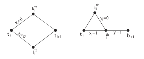
Figure 2: Two gadgets used to modify the reduction from Parity in the query complexity model to one for Inner Product in the communication complexity model. On the left the gadget used to replace the top $z_{i}=0$ edge in the graph from Figure 1, and on the right the gadget for the diagonal top to bottom $z_{i}=1$ edge.

5 Matching

The second graph problem we consider is deciding whether an $n\times n$ bipartite graph $G$ contains a perfect matching. We denote this problem by $\mbox{\sc Matching}_{n}$. First, we show that the above reduction from IP can be modified to also work for Matching.

Theorem 2.

$Q_{2}(\mbox{\sc Matching}_{n})\geq\Omega(n)$.

Proof.

Let $x\in\{0,1\}^{n}$ and $y\in\{0,1\}^{n}$ be respectively the inputs of Alice and Bob. As previously, we set $z=x\wedge y$, and observe again that the parity of $z$ is $\mbox{\sc IP}_{n}(x,y)$. We go back to the query world and the $2n$-vertex graph $G_{z}$ of Claim 1. Assume $n$ is odd. Then in case the parity of $z$ is odd, $G_{z}$ is a cycle of even length $2n$ and so has a perfect matching. On the other hand, in case the parity of $z$ is even, $G_{z}$ consists of two odd cycles and so has no perfect matching.

Now we again use gadgets to transfer this idea to a reduction from inner product to matching in the communication complexity setting. For simplicity we first describe the reduction where the edge sets of Alice and Bob can overlap. We then explain a modification to make them disjoint.

The vertices of the graph $G$ will consist of the $2n$ vertices $t_{i},b_{i}$ as in Figure  1 with the addition of $4n$ new vertices $k_{i}^{t},k_{i}^{b},\ell_{i}^{t},\ell_{i}^{b}$ for $i\in[n]$. For every $i$ there is a unique gadget on vertex set $\{t_{i},b_{i},k_{i}^{t},k_{i}^{b},\ell_{i}^{t},\ell_{i}^{b},t_{i+1},b_{i+1}\}$. The edges $\{k_{i}^{t},\ell_{i}^{b}\}$ and $\{k_{i}^{b},\ell_{i}^{t}\}$ are always present in the graph, and will be given to Alice. If $x_{i}=0$ then we give Alice the edges $\{t_{i},t_{i+1}\}$ and $\{b_{i},b_{i+1}\}$. If $y_{i}=0$ we do the same thing for Bob (this is where edges may overlap). If $x_{i}=1$ we give Alice the edges $\{t_{i},k_{i}^{t}\}$ and $\{b_{i},k_{i}^{b}\}$. If $y_{i}=1$ we give Bob the edges $\{t_{i+1},\ell_{i}^{t}\}$ and $\{b_{i+1},\ell_{i}^{b}\}$. This is illustrated in Figure 3.

Now in case the parity of $z$ is odd, we will have a cycle of even length, with possibly some additional disjoint edges and attached paths of length two. Thus there will be a perfect matching. In case the parity of $z$ is even, we will have two odd cycles, and again some additional disjoint edges or attached paths of length two. Suppose, by way of contradiction, that there is a perfect matching in this case. In case $x_{i}y_{i}=0$, this matching must include the edge $\{k_{i}^{t},\ell_{i}^{b}\}$, since at least one of these vertices has degree one, and similarly for $\{k_{i}^{b},\ell_{i}^{t}\}$. Thus a perfect matching in this case gives a perfect matching of two odd cycles, a contradiction.

To make the edge sets disjoint, we replace horizontal edges between vertex $i$ and $i+1$ by the gadget in the left of Figure 3. It can be seen that this does not change the properties used in the reduction.

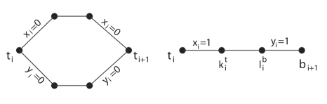
Figure 3: Two gadgets used to modify the reduction from Parity in the query complexity model to one for matching in the communication complexity model. On the right is the gadget for the top to bottom diagonal $z_{i}=1$ edge. On the left, the gadget used to replace the top $z_{i}=0$ horizontal edge in the graph from Figure 1 such that Alice and Bob receive disjoint sets of edges.

∎

Second, we show a non-trivial deterministic upper bound $D(\mbox{\sc Matching}_{n})=O(n^{3/2}\log n)$ by implementing a distributed version of the famous Hopcroft-Karp algorithm for finding a maximum-cardinality matching [HK73]. Let us first explain this algorithm in the standard non-distributed setting. The algorithm starts with an empty matching $M$, and in each iteration grows the size of $M$ until it can no longer be increased. It does this by finding, in each iteration, many augmenting paths. An augmenting path, relative to a matching $M$, is a path $P$ of odd length that starts and ends at “free” (= unmatched in $M$) vertices, and alternates non-matching with matching edges. Note that the symmetric difference of $M$ and $P$ is another matching, of size one greater than $M$. Each iteration of the Hopcroft-Karp algorithm does the following (using the notation of [HK73], we call the vertex sets of the bipartition $X$ and $Y$, respectively).

1. A breadth-first search (BFS) partitions the vertices of the graph into layers. The free vertices in $X$ are used as the starting vertices of this search, and form the initial layer of the partition. The traversed edges are required to alternate between unmatched and matched. That is, when searching for successors from a vertex in $X$, only unmatched edges may be traversed, while from a vertex in $Y$ only matched edges may be traversed. The search terminates at the first layer $k$ where one or more free vertices in $Y$ are reached.

2. All free vertices in $Y$ at layer $k$ are collected into a set $F$. That is, a vertex $v$ is put into $F$ iff it ends a shortest augmenting path (i.e., one of length $k$). The algorithm finds a maximal set of vertex-disjoint augmenting paths of length $k$. This set may be computed by depth-first search (DFS) from $F$ to the free vertices in $X$, using the BFS-layering to guide the search: the DFS is only allowed to follow edges that lead to an unused vertex in the previous layer, and paths in the DFS tree must alternate between unmatched and matched edges. Once an augmenting path is found that involves one of the vertices in $F$, the DFS is continued from the next starting vertex. After the search is finished, each of the augmenting paths found is used to enlarge $M$.

The algorithm stops when a new iteration fails to find another augmenting path, at which point the current $M$ is a maximal-cardinality matching. Hopcroft and Karp showed that this algorithm finds a maximum-cardinality matching using $O(\sqrt{n})$ iterations. Since each iteration takes time $O(n^{2})$ to implement, the overall time complexity is $O(n^{5/2})$.

Now consider what happens in a distributed setting, where Alice and Bob each have some of the edges of $G$. In this case, one iteration of the Hopcroft-Karp algorithm can be implemented by having each party perform as much of the search as possible within their graph, and then communicate the relevant vertices and edges to the other. To be more specific, the BFS is implemented as follows. For each level, first Alice scans the vertices on the given level and lists the set of vertices which belong to the next level due to edges seen by Alice, and then Bob lists the remaining vertices of the next level. When doing a DFS, first Alice goes forward as much as possible, then Bob follows. If Bob cannot continue going forward he gives the control back to Alice who will step back. Otherwise Bob goes forward as much as he can and then gives the control back to Alice who can either step back or continue going forward. During both types of search, when a new vertex is discovered Alice or Bob communicates the vertex as well as the edge leading to the new vertex. (Note that both the BFS and the DFS give algorithms of communication cost $\Theta(n\log n)$ for the constructive version of connectivity.)

Since each vertex needs to be communicated at most once per iteration, implementing one iteration thus takes $O(n\log n)$ bits of communication. Since there are $O(\sqrt{n})$ iterations, the whole procedure can be implemented using $O(n^{3/2}\log n)$ bits of communication. Finding the maximum-cardinality matching of course suffices for deciding if $G$ contains a perfect matching, so we get the same upper bound on $D(\mbox{\sc Matching}_{n})$ (strangely, we don’t know anything better when we allow randomization and quantum communication). We have proved:

Theorem 3.

$D(\mbox{\sc Matching}_{n})\leq O(n^{3/2}\log n)$.

5.1 Reducing communication by distributing Lovász’s algorithm?

In the usual setting of computation (not communication), Lovász [Lov79] gave a very elegant randomized method to decide whether a bipartite graph contains a perfect matching in matrix-multiplication time. Briefly, it works as follows. The determinant of an $n\times n$ matrix $A$ is

$$\det(A)=\sum_{\sigma\in S_{n}}\mbox{\rm sgn}(\sigma)\prod_{i=1}^{n}A_{i,\sigma(i)}.$$

This $\det(A)$ is a degree-$n$ polynomial in the matrix entries. Suppose we fix the $A_{ij}$ that equal 0, and replace the other $A_{ij}$ by variables $x_{ij}$. This turns $\det(A)$ into a polynomial $p(x)$ of degree $n$ in (at most) $n^{2}$ variables $x_{ij}$. Note that the monomial $\prod_{i=1}^{n}x_{i,\sigma(i)}$ vanishes iff at least one of the $A_{i,\sigma(i)}$ equals 0. Hence a graph $G$ has no perfect matching iff the polynomial $p(x)$ derived from its bipartite adjacency matrix $A$ is identically equal to 0. Testing whether a polynomial $p$ is identically equal to 0 is easy to do with a randomized algorithm: randomly choose values for the variables $x_{ij}$ from a sufficiently large field, and compute the value of the polynomial $p(r)$. If $p\equiv 0$ then $p(r)=0$, and if $p\not\equiv 0$ then $p(r)\neq 0$ with high probability by the Schwartz-Zippel lemma [Sch80, Zip79]. Since $p(x)$ is the determinant of an $n\times n$ matrix, which can be computed in matrix-multiplication time $O(n^{\omega})$, we obtain the same upper bound on the time needed to decide with high probability whether a graph contains a perfect matching.

One might hope that a distributed implementation of Lovász’s algorithm could improve the above communication protocol for matching, using randomization and possibly even quantum communication. Unfortunately this does not work, because it turns out that computing the determinant of an $n\times n$ matrix whose $n^{2}$ entries are distributed over Alice and Bob, takes $\Omega(n^{2})$ qubits of communication. In fact, even deciding whether the determinant equals 0 modulo 2 takes $\Omega(n^{2})$ qubits of communication. We show this by reduction from $\mbox{\sc IP}_{n^{2}}$. Let $\mathrm{DET}_{n}$ be the communication problem where Alice is given an $n$-by-$n$ Boolean matrix $X$, Bob an $n$-by-$n$ Boolean matrix $Y$, and the desired output is $\det(X\wedge Y)$, where $X\wedge Y$ is the bitwise AND of $X$ and $Y$.

Theorem 4.

$\Omega(n^{2})\leq Q_{2}(\mathrm{DET}_{n})$.

Proof.

As before, we first explain a reduction in the query world from Parity of $n^{2}$ bits to computing the determinant of a $(2n+2)\times(2n+2)$ matrix. The basic idea of the proof goes back to Valiant [Val79]. Say that we want to compute the parity of the bits of an $n^{2}$-bit string $Z$, and arrange the bits of $Z$ into an $n$-by-$n$ matrix. We construct a directed bipartite graph $G_{Z}$ with $2n+2$ vertices, $n+1$ on each side (we will refer to these as left-hand side and right-hand side). Label the vertices on the left-hand side as $t$ and $\ell_{i}$ for $i\in[n]$, and those on the right-hand side as $s$ and $r_{i}$ for $i\in[n]$. For every $i\in[n]$, we add the edges $(s,\ell_{i})$ and $(r_{i},t)$. For every $(i,j)$ with $Z(i,j)=1$ we put an edge $(\ell_{i},r_{j})$. Finally we put the edge $(t,s)$, and self-loops are added to all vertices but $s$ and $t$.

Claim 2.

$\det(G_{Z})=-|Z|$.

Proof.

Note that

$$\det(G_{Z})=\sum_{\sigma}(-1)^{\chi(\sigma)}\prod_{i}G_{Z}(i,\sigma(i)).$$

Consider a permutation that contributes to this sum. In this case, $\sigma(\ell_{i})=r_{j}$ for some $i,j$ for which $Z(i,j)=1$. We then must have $\sigma(r_{j})=t,\sigma(t)=s,\sigma(s)=\ell_{i}$ and that $\sigma$ fixes all other vertices. The sign of this permutation is negative, and we get such a contribution for every $i,j$ such that $Z(i,j)=1$. ∎

Now again we transfer this reduction to the communication complexity setting by means of a gadget. Say that Alice has $X$, an $n$-by-$n$ matrix and similarly Bob has $Y$ and they want to compute $|X\wedge Y|\bmod 2$. We will actually count the number of zeros in $X\wedge Y$, which clearly then allows us to know the number of ones and so the parity.

We give Alice the set of edges $E_{A}$ and Bob the set of edges $E_{B}$. Unlike in the previous reductions, in this case $E_{A}$ and $E_{B}$ will not be disjoint (we do not know how to do the reduction with disjoint $E_{A},E_{B}$). Put $(s,\ell_{i}),(\ell_{i},\ell_{i})\in E_{A}$ for all $i\in[n]$ and similarly $(t,r_{i}),(r_{i},r_{i})\in E_{B}$ for all $i\in[n]$. For all $(i,j)$ where $X(i,j)=0$ put $(\ell_{i},r_{j})\in E_{A}$, and similarly for all $(i,j)$ where $Y(i,j)=0$ put $(\ell_{i},r_{j})\in E_{B}$. Thus in $E_{A}\cup E_{B}$ there is an edge $(\ell_{i},r_{j})$ if and only if $X(i,j)Y(i,j)=0$. Thus by Claim 2 from the determinant of the graph with edges $E_{A}\cup E_{B}$ we can determine the number of zeros in $X\wedge Y$.∎

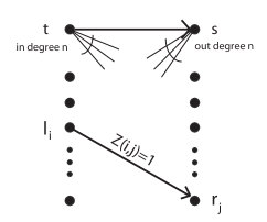
Figure 4: The construction of the graph $G_{Z}$. Self-loops omitted for clarity.

6 Eulerian tour

An Eulerian tour in a graph $G$ is a cycle that goes through each edge of the graph exactly once. A well-known theorem of Euler states that $G$ has such a tour iff it is connected and all its vertices have even degree. Denote the corresponding communication complexity problem for $n$-vertex graphs by $\mbox{\sc Euler}_{n}$. Note that when the sets $E_{A}$ and $E_{B}$ are allowed to overlap, deciding if the degree $\deg(v)$ of a fixed vertex $v\in[n]$ is even is essentially equivalent to $\mbox{\sc IP}_{n-1}$, as follows. Let $x\in\{0,1\}^{n-1}$ be the characteristic vector of the neighbors of $v$ in $E_{A}$, and $y\in\{0,1\}^{n-1}$ the same for $E_{B}$, then we have $\deg(v)=|x\vee y|=|x|+|y|-|x\wedge y|$. Since Alice and Bob can send each other the numbers $|x|$ and $|y|$ using a negligible $\log n$ bits, computing $deg(v)\bmod 2$ is essentially equivalent to computing $|x\wedge y|\bmod 2=\mbox{\sc IP}_{n-1}(x,y)$.

Now we show how to embed into $\mbox{\sc Euler}_{3n+4}$ an $\mbox{\sc OR}_{n}$ of disjoint $\mbox{\sc IP}_{n}$’s. As usual, we first explain the reduction in the query world. For $i\in[n]$, let $z^{i}\in\{0,1\}^{n}$, and suppose that we want to compute $\mbox{\sc OR}_{n}(|z^{1}|\bmod 2,\ldots,|z^{n}|\bmod 2)$. We construct a graph $G$ with $n+2$ left vertices $\ell_{i}$ and $n+2$ right vertices $r_{i}$ for $0\leq i\leq n+1$, and $n$ middle vertices $m_{i}$ for $i\in[n]$. Independently from the strings $z^{i}$, the graph $G$ always has the edges $\{\ell_{i},\ell_{i+1}\}$ and $\{r_{i},r_{i+1}\}$ for $0\leq i\leq n$ and the edges $\{m_{i},m_{i+1}\}$ for $1\leq i\leq n-1$. It also contains the following 5 edges: $\{\ell_{0},m_{1}\},\{r_{0},m_{1}\},\{\ell_{n+1},m_{n}\},\{r_{n+1},m_{n}\},\{m_{1},m_{n}\}.$ We call these edges fixed edges. Finally, for every $(i,j)$ with $z^{i}_{j}=1$ we add the edges $\{\ell_{i},m_{j}\}$ and $\{r_{i},m_{j}\}$. Observe that $G$ is already connected by the fixed edges. See Figure 5 for an illustration.

Claim 3.

$G$ is Eulerian if and only if $\mbox{\sc OR}_{n}(|z^{1}|\bmod 2,\ldots,|z^{n}|\bmod 2)=0$.

Proof.

In the subgraph restricted to the fixed edges every vertex has even degree. Therefore we can restrict our attention to the degrees with respect to the remaining edges that depend on the values $z^{i}_{j}$. All the middle vertices have even degrees since for all $(i,j)$, we add 0 or 2 edges adjacent to $m_{j}$. For every $i\in[n],$ the degrees of $\ell_{i}$ and $r_{i}$ are the same since we add the edge $\{\ell_{i},m_{j}\}$ exactly when we add the edge $\{r_{i},m_{j}\}$. The degree of $\ell_{i}$ is the Hamming weight of $z^{i}$. Therefore $G$ is Eulerian iff $|z^{i}|$ is even for all $i\in[n]$. ∎

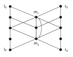
Figure 5: Illustration of the graph to reduce OR of parities to Eulerian tour in the query model. In this example, $n=3$ and $z^{1}=010,z^{2}=101,z^{3}=000$.

The transfer of this reduction to the communication complexity setting is quite simple. Suppose that for each $i\in[n]$ Alice has string $x^{i}\in\{0,1\}^{n}$, and Bob has $y^{i}\in\{0,1\}^{n}$, and they want to compute the function $\mbox{\sc OR}_{n}(\mbox{\sc IP}_{n}(x^{1},y^{1}),\ldots,\mbox{\sc IP}_{n}(x^{n},y^{n}))$. Let us suppose that $n$ is even, then $\mbox{\sc IP}_{n}(x^{i},y^{i})=\sum_{j}(\bar{x}^{i}_{j}\vee\bar{y}^{i}_{j})$. For all $(i,j)$ such that $x^{i}_{j}=0$ we put the edges $\{\ell_{i},m_{j}\}$ and $\{r_{i},m_{j}\}$ in $E_{A}$, and similarly, for $y^{i}_{j}=0$ we put the edges $\{\ell_{i},m_{j}\}$ and $\{r_{i},m_{j}\}$ in $E_{B}$. Thus in $E_{A}\cup E_{B}$ the edges $\{\ell_{i},m_{j}\}$ and $\{r_{i},m_{j}\}$ exist if and only if $\bar{x}^{i}_{j}\vee\bar{y}^{i}_{j}=1$. Therefore, by Claim 3 $\mbox{\sc OR}_{n}(\mbox{\sc IP}_{n}(x^{1},y^{1}),\ldots,\mbox{\sc IP}_{n}(x^{n},y^{n}))=0$ if and only if $G$ is Eulerian.

We can easily reduce $\mbox{\sc Disj}_{n^{2}}$ on $n^{2}$-bit instances with intersection size 0 or 1 to $\mbox{\sc OR}_{n}\circ\mbox{\sc IP}_{n}$. Since even that special case of $\mbox{\sc Disj}_{n^{2}}$ requires linear classical communication [Raz92], we obtain a tight lower bound $R_{2}(\mbox{\sc Euler}_{n})=\Omega(n^{2})$.

The quantum communication complexity of $\mbox{\sc OR}_{n}(\mbox{\sc IP}_{n}(x^{1},y^{1}),\ldots,\mbox{\sc IP}_{n}(x^{n},y^{n}))$ is $\Omega(n^{3/2})$. This follows because for any $f(g(x^{1},y^{1}),\ldots,g(x^{n},y^{n}))$ where $g$ is strongly balanced (meaning that all rows and columns in the communication matrix $M(x,y)=(-1)^{g(x,y)}$ sum to zero), the quantum communication complexity of $f$ is at least the approximate polynomial degree of $f$, times the discrepancy bound of $g$ [LZ10, Cor. 3]. In our case, $\mbox{\sc OR}_{n}$ has approximate degree $\Omega(\sqrt{n})$ and $\mbox{\sc IP}_{n}$ contains a $2^{n-1}$-by-$2^{n-1}$ strongly balanced submatrix with discrepancy bound $\Omega(n)$. Thus we get $Q_{2}(\mbox{\sc Euler}_{n})\geq Q_{2}(\mbox{\sc OR}_{n}\circ\mbox{\sc IP}_{n})\geq\Omega(n^{3/2})$.

This quantum lower bound is in fact tight: we first decide if $G$ is connected using $O(n\log n)$ bits of communication (Section 4), and if so then we use the Aaronson-Ambainis protocol to search for a vertex of odd degree (deciding whether a given vertex has odd degree can be done deterministically with $O(n)$ bits of communication). Thus we have:

Theorem 5.

$R_{2}(\mbox{\sc Euler}_{n})=\Theta(n^{2})$ and $Q_{2}(\mbox{\sc Euler}_{n})=\Theta(n^{3/2})$.

7 Other problems

In this section we look at the quantum and classical communication complexity of a number of other graph properties. Most results here are easy observations based on previous work, but worth making nonetheless.

7.1 Triangle-finding

Suppose we want to decide whether $G$ contains a triangle. Papadimitriou and Sipser [PS84, pp. 266–7] gave a reduction from $\mbox{\sc Disj}_{m}$ to $\mbox{\sc Triangle}_{n}$ for $m=\Omega(n^{2})$, which implies $R_{2}(\mbox{\sc Triangle}_{n})=\Theta(n^{2})$. Since we know that $Q_{2}(\mbox{\sc Disj}_{m})=\Theta(\sqrt{m})$, it also follows that $Q_{2}(\mbox{\sc Triangle}_{n})=\Omega(n)$.

This quantum lower bound is actually tight, which can be seen as follows. First Alice checks if there already is a triangle within the edges $E_{A}$, and Bob does the same for $E_{B}$. If not, then Alice defines the set of edges $S_{A}=\{(a,b)\mid\exists~{}c~{}s.t.~{}(a,c),(b,c)\in E_{A}\}$ which would complete a triangle for her, and uses the Aaronson-Ambainis protocol to try to find one among Bob’s edges (i.e., she searches for an edge in $S_{A}\cap E_{B}$). Since $|S_{A}|\leq{n\choose 2}$, this process will find a triangle if Alice already holds two of its edges, using $O(n)$ qubits of communication. Bob does the same from his perspective. If $G$ contains a triangle, then either Alice or Bob has at least two edges of this triangle. Hence this protocol will find a triangle with high probability if one exists, using $O(n)$ qubits of communication. Thus we have:

Theorem 6.

$R_{2}(\mbox{\sc Triangle}_{n})=\Theta(n^{2})$ and $Q_{2}(\mbox{\sc Triangle}_{n})=\Theta(n)$.

7.2 Bipartiteness

Deterministic protocols can decide whether a given graph $G$ is bipartite using $O(n\log n)$ bits of communication, as follows. Being bipartite is equivalent to being 2-colorable. Alice starts with some vertex $v_{1}$, colors it red, and colors all of its neighbors (within $E_{A}$) blue. Then she communicates all newly-colored vertices and their colors to Bob. Bob continues coloring the neighbors of $v_{1}$ blue, and once he’s done he communicates the newly-colored vertices and their colors to Alice. If all vertices have been colored then Alice stops, otherwise she chooses an uncolored neighbor $v_{2}$ of a blue vertex, colors $v_{2}$ red, and continues as above coloring $v_{2}$’s neighbors blue. A connected graph is 2-colorable iff this process terminates without encountering a vertex colored both red and blue (if the graph is not connected then Alice and Bob can treat each connected component separately). Since each vertex will be communicated at most once, the whole process takes $O(n\log n)$ bits.

Babai et al. [BFS86, Section 9] state a reduction from $\mbox{\sc IP}_{n}$ to bipartiteness, which implies a near-matching quantum lower bound $Q_{2}(\mbox{\sc Bipartite}_{n})=\Omega(n)$.

Theorem 7.

$\Omega(n)\leq Q_{2}(\mbox{\sc Bipartite}_{n})\leq D(\mbox{\sc Bipartite}_{n})\leq O(n\log n)$.

7.3 Planarity

Duris and Pudlák [DP89] exhibited a deterministic protocol with $O(n\log n)$ bits of communication for deciding whether a graph $G$ is planar (i.e., whether it can be drawn in the plane without intersecting edges). Babai et al. [BFS86, Section 9] state a reduction from $\mbox{\sc IP}_{n}$ to planarity, which implies a near-matching quantum lower bound $Q_{2}(\mbox{\sc Planar}_{n})=\Omega(n)$.

8 Conclusion and open problems

In this paper we studied the communication complexity (quantum and classical) of a number of natural graph properties, obtaining nearly tight bounds for many of them. We mention a few open problems:

• For Connected, can we improve the quantum upper bound from the trivial $O(n\log n)$ to $O(n)$, matching the lower bound? One option would be to run a distributed version of the $O(n)$-query quantum algorithm of Dürr et al. [DHHM06], but this involves a classical preprocessing phase that seems to require $O(n\log n)$ communication. Another option would be to run some kind of quantum random walk on the graph, starting from a random vertex, and test whether it converges to a superposition of all vertices.

• For Matching, can we show that the deterministic $O(n^{3/2}\log n)$-bit protocol is essentially optimal, for instance by means of a $2^{\Omega(n^{3/2})}$ lower bound on the rank of the associated communication matrix? Can we improve this upper bound using randomization and/or quantum communication, possibly matching the $Q_{2}(\mbox{\sc Matching}_{n})=\Omega(n)$ lower bound?

• Can we extend the $D(\mbox{\sc Matching}_{n})\leq O(n^{3/2}\log n)$ bound to general graphs?

References

- [AA05] S. Aaronson and A. Ambainis. Quantum search of spatial regions. Theory of Computing, 1(1):47–79, 2005. Earlier version in FOCS’03. quant-ph/0303041.
- [BCW98] H. Buhrman, R. Cleve, and A. Wigderson. Quantum vs. classical communication and computation. In Proceedings of 30th ACM STOC, pages 63–68, 1998. quant-ph/9802040.
- [BFS86] L. Babai, P. Frankl, and J. Simon. Complexity classes in communication complexity theory. In Proceedings of 27th IEEE FOCS, pages 337–347, 1986.
- [CDNT98] R. Cleve, W. van Dam, M. Nielsen, and A. Tapp. Quantum entanglement and the communication complexity of the inner product function. In Proceedings of 1st NASA QCQC conference, volume 1509 of Lecture Notes in Computer Science, pages 61–74. Springer, 1998. quant-ph/9708019.
- [CK07] A. Chakrabarti and S. Khot. Improved lower bounds on the randomized complexity of graph properties. Random Structures and Algorithms, 30(3):427–440, 2007. Earlier version in ICALP’01.
- [CW90] D. Coppersmith and S. Winograd. Matrix multiplication via arithmetic progressions. Journal of Symbolic Computation, 9(3):251–280, 1990. Earlier version in STOC’87.
- [DHHM06] C. Dürr, M. Heiligman, P. Høyer, and M. Mhalla. Quantum query complexity of some graph problems. SIAM Journal on Computing, 35(6):1310–1328, 2006. Earlier version in ICALP’04.
- [DHK+11] A. DasSarma, S. Holzer, L. Kor, A. Korman, D. Nanongkai, G. Pandurangan, D. Peleg, and R. Wattenhofer. Distributed verification and hardness of distributed approximation. In Proceedings of 43rd ACM STOC, pages 363–372, 2011.
- [DP89] P. Duris and P. Pudlák. On the communication complexity of planarity. In Proceedings of 7th Fundamentals of Computation Theory (FCT’89), pages 145–147, 1989.
- [EKNP12] M. Elkin, H. Klauck, D. Nanongkai, and G. Pandurangan. Quantum Distributed Network Computing: Lower Bounds and Techniques. Manuscript, 2012.
- [For01] J. Forster. A linear lower bound on the unbounded error probabilistic communication complexity. In Proceedings of 16th IEEE Conference on Computational Complexity, pages 100–106, 2001.
- [Haj91] P. Hajnal. An lower bound on the randomized complexity of graph properties. Combinatorica, 11:131–143, 1991. Earlier version in Structures’90.
- [HF98] M. R. Henzinger and M. L. Fredman. Lower bounds for fully dynamic connectivity problems in graphs. Algorithmica, 22(3):351–362, 1998.
- [HK73] J. E. Hopcroft and R. M. Karp. An algorithm for maximum matchings in bipartite graphs. SIAM Journal on Computing, 2(4):225–231, 1973. Earlier version in FOCS’71.
- [HMT88] A. Hajnal, W. Maass, and G. Turán. On the communication complexity of graph properties. In Proceedings of 20th ACM STOC, pages 186–191, 1988.
- [KN97] E. Kushilevitz and N. Nisan. Communication Complexity. Cambridge University Press, 1997.
- [Kre95] I. Kremer. Quantum communication. Master’s thesis, Hebrew University, Computer Science Department, 1995.
- [KS92] B. Kalyanasundaram and G. Schnitger. The probabilistic communication complexity of set intersection. SIAM Journal on Discrete Mathematics, 5(4):545–557, 1992. Earlier version in Structures’87.
- [Lov79] L. Lovász. On determinants, matchings, and random algorithms. In Proceedings of 2nd Fundamentals of Computation Theory (FCT’79), pages 565–574, 1979.
- [LZ10] T. Lee and S. Zhang. Composition theorems in communication complexity. In Proceedings of the 37th ICALP, pages 475–489, 2010. arXiv:1003.1443.
- [NC00] M. A. Nielsen and I. L. Chuang. Quantum Computation and Quantum Information. Cambridge University Press, 2000.
- [PS84] C. H. Papadimitriou and M. Sipser. Communication complexity. Journal of Computer and System Sciences, 28(2):260–269, 1984. Earlier version in STOC’82.
- [Raz92] A. Razborov. On the distributional complexity of disjointness. Theoretical Computer Science, 106(2):385–390, 1992.
- [Raz03] A. Razborov. Quantum communication complexity of symmetric predicates. Izvestiya of the Russian Academy of Sciences, mathematics, 67(1):159–176, 2003. quant-ph/0204025.
- [RV76] R. Rivest and S. Vuillemin. On recognizing graph properties from adjacency matrices. Theoretical Computer Science, 3:371–384, 1976.
- [Sch80] J. T. Schwartz. Fast probabilistic algorithms for verification of polynomial identities. Journal of the ACM, 27:701–717, 1980.
- [Sto10] A. Stothers. On the Complexity of Matrix Multiplication. PhD thesis, University of Edinburgh, 2010.
- [Val79] L. Valiant. Completeness classes in algebra. In Proceedings of 11th ACM STOC, pages 249–261, 1979.
- [Wil12] V. Vassilevska Williams. Multiplying matrices faster than Coppersmith-Winograd. In Proceedings of 44th ACM STOC, 2012. To appear.
- [Wol02] R. de Wolf. Quantum communication and complexity. Theoretical Computer Science, 287(1):337–353, 2002.
- [Zip79] R. E. Zippel. Probabilistic algorithms for sparse polynomials. In Proceedings of EUROSAM 79, volume 72 of Lecture Notes in Computer Science, pages 216–226, 1979.