The SPLASH Survey:
Kinematics of Andromeda’s Inner Spheroid

Abstract

The combination of large size, high stellar density, high metallicity, and Sérsic surface brightness profile of the spheroidal component of the Andromeda galaxy (M31) within $R_{\rm proj}\sim 20$ kpc suggest that it is unlike any subcomponent of the Milky Way. In this work we capitalize on our proximity to and external view of M31 to probe the kinematical properties of this “inner spheroid.” We employ a Markov chain Monte Carlo (MCMC) analysis of resolved stellar kinematics from Keck /DEIMOS spectra of $5651$ red giant branch stars to disentangle M31’s inner spheroid from its stellar disk. We measure the mean velocity and dispersion of the spheroid in each of five spatial bins after accounting for a locally cold stellar disk as well as the Giant Southern Stream and associated tidal debris. For the first time, we detect significant spheroid rotation ($v_{\rm rot}\sim 50~{}\rm km~{}s^{-1}$) beyond $R_{\rm proj}\sim 5$ kpc. The velocity dispersion decreases from about $140\rm~{}km~{}s^{-1}$ at $R_{\rm proj}=7$ kpc to $120\rm~{}km~{}s^{-1}$ at $R_{\rm proj}=14$ kpc, consistent to $2\sigma$ with existing measurements and models. We calculate the probability that a given star is a member of the spheroid and find that the spheroid has a significant presence throughout the spatial extent of our sample. Lastly, we show that the flattening of the spheroid is due to velocity anisotropy in addition to rotation. Though this suggests that the inner spheroid of M31 more closely resembles an elliptical galaxy than a typical spiral galaxy bulge, it should be cautioned that our measurements are much farther out ($2-14~{}r_{\rm eff}$) than for the comparison samples.

1. INTRODUCTION

The elegant progression of the Hubble sequence from ellipticals to spirals demonstrates that galaxy morphology can be described in large part based on the relative importance of spheroid and disk subcomponents. While it is now clear that the simple evolutionary path from elliptical “early-type” to disk-dominated “late-type” galaxies that Hubble (1936) originally proposed is incorrect, the physical origin of the Hubble sequence and the formation of and relationship between the different structural subcomponents remain subjects of vigorous research.

The central spheroids of spiral galaxies fall into two categories, which can be explained by distinct formation mechanisms as reviewed by Kormendy & Kennicutt (2004). Classical bulges, which are typically described as elliptical galaxy analogs with random stellar velocity distributions, large velocity dispersions, and $r^{1/4}$ de Vaucouleurs surface brightness profiles, are likely formed through violent merger/accretion events. Pseudobulges, which are more flattened, have more ordered kinematics, and have roughly exponential brightness cutoffs (or, more generally, Sérsic profiles with low $n_{\rm S\acute{e}rsic}$ values) are likely formed through secular heating of the disk. More detailed observations, yielding constraints on the structure and dynamics of bulges, will lead to a clearer understanding of possible formation scenarios.

Any study of the inner regions of a galaxy is complicated by the presence of several spatially overlapping structural subcomponents, such as the disk, spheroid, and halo. Deconvolving these subcomponents to reveal the behavior of a single one is difficult. Traditionally, codes such as GALFIT (Peng et al., 2002) or GIM2D (Simard, 2002) are employed to fit galactic integrated light profiles with the sum of a Sérsic bulge and exponential disk (e.g. Courteau, 1996; Courteau et al., 2011). This technique is the only possible method for characterizing the structure of distant galaxies, but it suffers from strong assumptions about the characteristic light profiles of bulges and disks. In addition, degeneracy in the best-fit derived parameters can cloud interpretation of the results.

Resolved stellar kinematics offer a complementary approach to structural deconvolution of the nearest galaxies. Instead of assuming specific surface brightness profiles of disks and spheroids, one must only make the geometrical argument that a stable disk – a thin, flat structure – is kinematically colder (has a higher $v_{\rm rot}/\sigma_{v}$) than a stable spheroid. Separate components can then be identified and characterized by their distinct stellar velocity distributions. The proximity of Andromeda (M31) at about 785 kpc (e.g., McConnachie et al., 2008) renders it the only large spiral galaxy other than the Milky Way (MW) where detailed photometric and kinematical observations are possible with current observing facilities.

We use resolved stellar kinematics to study M31’s kinematically hot “inner spheroid” at projected radii of 2–20 kpc. Any description of this region – or that in the the intermediate region of any large galaxy – is necessarily complex; the literature is full of vocabulary such as “bulge,” “spheroid,” “inner spheroid,” “outer spheroid,” “disk,” “thin disk,” “thick disk,” “extended disk,” and so on. There is not yet a consensus on the best combination of these nouns to represent M31. For the purposes of this paper, we use the word “spheroid” to describe a kinematically hot component: some combination of bulge, halo, and/or any other spheroidal component. Likewise, we refer to the kinematically colder population as the “disk,” where this term includes any distinct disk components that may be present, such as the thin, thick or extended disks.

Despite the possibility of multiple components, the disk is likely to be locally kinematically cold. Collins et al. (2011) claim that M31’s stellar disk at $r_{\rm proj}\sim$10–40 kpc consists of a cold thin disk and a warm thick disk, as is the case for the MW. Given that most of our fields are closer to M31’s center than the innermost field of Collins et al. (2011), and given their finding that the thin disk has twice the density of the thick disk and a shorter radial scale length, we expect the cold thin disk to dominate the stellar disk population in our fields. Similarly, Ibata et al. (2005) suggest that no more than about 10% of the total disk luminosity may be due to an extended disk component which also lags the cold disk. Though we do not know a priori the relative contributions of the thin, thick and extended disks, in § 4.2 we show that our assumption of a dominant thin component is justified for the purposes of measuring the kinematical parameters of the inner spheroid.

Unlike the case of its stellar disk, M31’s inner spheroid has no analog in the MW and is therefore of great interest. The spheroidal system at these radii in the MW is relatively metal-poor ($\langle Fe/H\rangle\sim-1.6$; Carollo et al., 2007), is composed entirely of old stars, and has a power-law spatial density profile of the form $r_{\rm deproj}^{-3}$, which corresponds to an $r^{-2}$ power-law surface brightness profile. Models such as those proposed by Bullock & Johnston (2005) and Zolotov et al. (2010) suggest that the MW halo represents a population of accreted dwarf satellite galaxies. In contrast, the inner spheroid in M31 more closely resembles a bulge than a halo. It is more metal-enhanced than the MW halo, with [Fe/H] $\sim-0.7$ (Kalirai et al., 2006a), and has a Sérsic surface brightness profile with $n_{\rm S\acute{e}rsic}\sim 2$–4 (Pritchet & van den Bergh, 1994; Guhathakurta et al., 2005; Courteau et al., 2011). In addition, the stellar population of M31’s spheroid is younger than that of the MW inner halo on average, with $40\%$ of the stars younger than $10$ Gyr (Brown et al., 2006), and the stellar density is also significantly higher than that at an equivalent location in the MW (Reitzel et al., 1998).

The inner spheroid straddles territory between two well-studied components of the spheroid: the classical and boxy bulges interior to $\sim 1~{}\rm kpc$ (Athanassoula & Beaton, 2006; Beaton et al., 2007; Courteau et al., 2011), and the outer halo which dominates past $R_{\rm proj}\sim 30\rm~{}kpc$ (e.g. Guhathakurta et al., 2005; Irwin et al., 2005; Ibata et al., 2007). In the central kpc, where the density is too high for resolved stellar population spectroscopy, Saglia et al. (2010) analyzed integrated-light kinematics to reveal a bulge rotation speed of $70~{}\rm km~{}s^{-1}$ and a velocity dispersion of $140~{}\rm km~{}s^{-1}$ at $R_{\rm proj}=1.1~{}\rm kpc$ on the major axis. However, they cautioned that this measurement is contaminated by the kinematically cold disk which may contribute nearly a third of the light at this radius.

Farther out in M31’s halo, kinematical surveys of the resolved stellar population using the Keck/DEIMOS multiobject spectrograph have mapped the cold substructure, as well as the underlying smooth virialized population, out to $R_{\rm proj}>150$ kpc (Guhathakurta et al., 2005; Chapman et al., 2006; Kalirai et al., 2006a; Gilbert et al., 2007, 2009). Chapman et al. (2006) compiled kinematics of $\sim 1200$ red giant branch (RGB) halo stars in scattered fields between $R_{\rm proj}=$8 and 70 kpc. Using a windowing technique to eliminate stars whose velocities were consistent with that of the disk, they found that the velocity dispersion of the remaining population decreased radially outwards: $\sigma_{v}(R_{\rm proj})=(152-0.9~{}R_{\rm proj}\rm~{}kpc^{-1})~{}km~{}s^{-1}$. Subsequently, as part of the Spectroscopic and Panchromatic Landscape of Andromeda’s Stellar Halo (SPLASH) survey, Gilbert et al. (2007) fit a double Gaussian profile to the velocity distribution of RGB stars in a large contiguous region along the southeastern minor axis of the galaxy and measured a constant velocity dispersion of $128.9~{}\rm km~{}s^{-1}$ between $R_{\rm proj}=10$ and $30\rm~{}kpc$.

In recent years, the focus of SPLASH has migrated inwards, first to target the dwarf galaxies Andromeda I and Andromeda X (Tollerud, 2011), NGC 205 (Geha et al., 2006; Howley et al., 2008) and M32 (Howley et al., 2012), and now towards the disk- and bulge-dominated inner regions of M31. The majority of the data analyzed in the present paper come from the most crowded area targeted to date: a large contiguous disk-dominated area on the NE major axis with $R_{\rm proj}=2$–19 kpc. This area was selected to overlap the coverage of the Panchromatic Hubble Andromeda Treasury (PHAT) survey, a five-year Hubble Space Telescope (HST) MultiCycle Treasury (MCT) program that began in 2010 (Dalcanton et al., 2012).

The disk and spheroid share the inner regions of the galaxy with remnants of tidally disrupted galaxies. The dominant features in star-count maps of the 2–20 kpc region are the Giant Southern Stream (GSS; the remnant of a tidally stripped satellite galaxy) and the shelves (sharp edges in stellar density) created by it (Ibata et al., 2001; Fardal et al., 2007). Both the GSS and a “secondary stream,” which is cospatial with the GSS but separated by $100~{}\rm km~{}s^{-1}$ in velocity, have been kinematically detected in multiple fields south of M31 (Kalirai et al., 2006b; Gilbert et al., 2009). Fardal et al. (2007) identified the northern extension of the stream in the Chapman et al. (2006) and Ibata et al. (2005) sample of RGBs and in the planetary nebulae of Merrett et al. (2006).

There are two principal challenges to a resolved stellar population kinematical study of the crowded inner spheroid of M31. First, we must select intended stellar targets whose spectra are least likely to be contaminated by close (in projection) stellar neighbors. Second, we must disentangle the stellar disk from the spheroid population we wish to characterize. This is especially important in disk-dominated fields, where fewer than $20\%$ of the stars may belong to the spheroid. Note that though a large part of this paper will focus on accounting for the disk contribution, our analysis method is designed to elucidate the nature of the inner spheroid rather than the disk. We do not attempt to make a statement here about the rotation curve of the stellar disk or the presence of a thick disk. We plan to analyze these components in a future paper.

This paper is organized as follows. In § 2 we explain our target selection techniques, spectroscopic observations and radial velocity extraction. In § 3 we describe our method for isolating and characterizing the spheroid velocity distribution in each of five spatial bins. In § 4 we discuss the implications of our results; finally, we summarize our findings in § 5.

2. OBSERVATIONS

Our data set for this project is a compilation of three sets of RGB spectra, two of which are presented here for the first time. A detailed technical description of the spectroscopic slitmask design and data reduction is given in Howley et al. (2012). In this section, we describe the target selection criteria for the different data sets and give an overview of the data acquisition and reduction methods common to all the observations.

In § 2.1, we outline the three data sets used in this paper. In § 2.2, we describe the source catalogs from which we select our spectroscopic targets. In § 2.3, we explain our target selection criteria. In § 2.4, we provide the observing details. In § 2.5, we give a rundown of the data reduction process. In § 2.6 and § 2.7, we measure velocities of individual stars and determine the quality of those measurements, respectively. Finally, in § 2.8, we discuss the detection and velocity measurement of serendipitously detected stars.

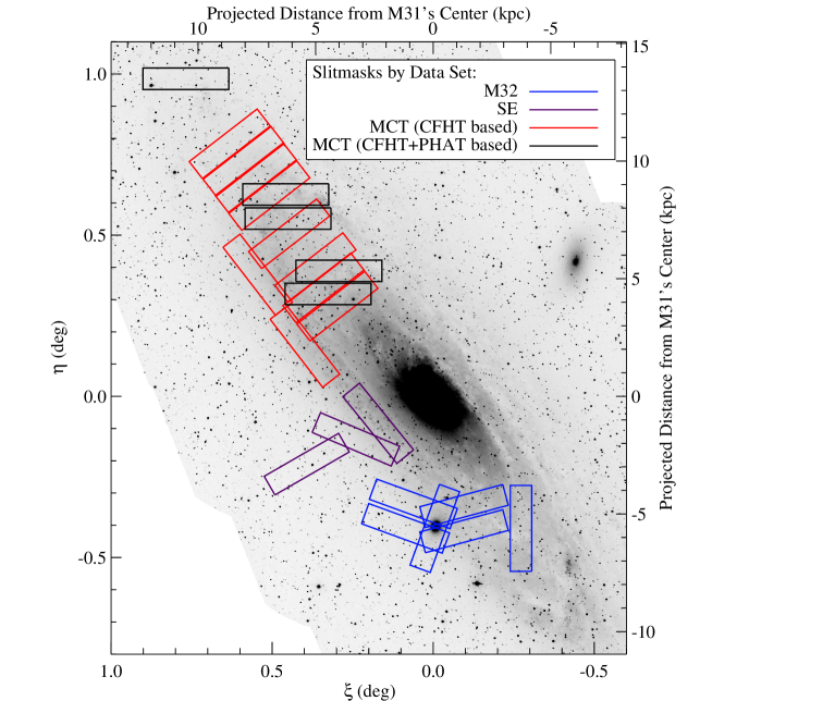
Figure 1.— Twenty-four Keck/DEIMOS multiobject slitmasks overlaid on the Choi et al. (2002) KPNO Burrell Schmidt $B$-band mosaic image of M31. Colored rectangles outline the slitmasks from the different data sets: SE (violet), M32 (blue), and MCT (red and black, respectively, for slitmasks for which target selection was based on only the ground-based CFHT/MegaCam photometry/astrometry catalog versus slitmasks for which target selection was based on a combination of the PHAT and CFHT/MegaCam photometry/astrometry catalogs).

2.1. Data Sets

The spatial coverage of our three data sets is shown in Figure 1. Each rectangular outline represents a Keck/DEIMOS slitmask, which covers approximately $16^{\prime}\times 4^{\prime}$ and yields 200–270 useful spectra. (The actual footprint of a DEIMOS slitmask is not perfectly rectangular.) The SE data sets consists of three slitmasks oriented along the eastern minor axis of M31 (violet in Figure 1). The M32 data set includes the five slitmasks covering the compact elliptical galaxy M32 directly south of M31 and one slitmask on the SW major axis (blue in Figure 1). The SE and M32 data sets were observed during the 2007 and 2008 fall seasons.

Our newest data set, from October 2010, covers a portion of M31’s northeastern major axis spanning the projected radial range $0.33^{\circ}$–$1.38^{\circ}$ or 2–19 kpc from the center of M31 in the plane of the disk (red and black in Figure 1). Five of these 15 slitmasks (black) were chosen to maximally overlap the regions of existing photometry from the first year of the PHAT program.

The pre-imaging and reduction processes are identical for all three data sets. The primary difference in data acquisition is in the target selection: isolated sources are hand-selected for the SE and M32 slitmasks from a single monochromatic ground-based source catalog (Howley et al., 2012), while we use an automated series of statistical techniques as well as limited color information from the PHAT survey to choose targets for the MCT slitmasks.

Table 1Keck/DEIMOS Multiobject Slitmask Exposures

Mask	Observation	$\alpha$ [J2000]	$\delta$ [J2000]	P.A.	$t_{\rm{exp}}$	Seeing	No. of	No. of Usable	No. of Usable
Name	Date (UT)	(h:m:s)	(∘:′:′′)	(∘)	(min)	FWHM	Slits	Target Velocities	Velocities of
								(Success Rate)	Serendipitously Detected
									Stars
M32_1	2007 Nov 14	00 42 38.28	$+$40 51 34.0	$+$160.0	2$\times$20	$0\farcs 5$	199	188 (94%)	72
M32_2	2008 Aug 03	00 43 03.82	$+$40 55 07.7	$+$70.0	3$\times$20	$0\farcs 6$	189	166 (88%)	27
M32_3	2008 Aug 03	00 43 11.60	$+$40 52 34.7	$-$110.0	3$\times$20	$0\farcs 7$	203	132 (65%)	10
M32_4	2008 Aug 04	00 42 13.87	$+$40 54 44.2	$+$105.0	3$\times$20	$0\farcs 6$	165	137 (83%)	119
M32_5	2008 Aug 04	00 42 13.88	$+$40 52 02.6	$-$75.0	3$\times$20	$0\farcs 6$	177	152 (86%)	72
M32_6	2008 Aug 31	00 41 20.41	$+$41 51 32.2	0.0	3$\times$20 $+$ 1$\times$10	$0\farcs 7$	169	152 (90%)	128
SE7	2008 Sept 01	00 43 38.74	$+$41 10 17.4	$+$39.0	2$\times$10	$0\farcs 8$	170	148 (87%)	50
SE8	2008 Sept 30	00 44 00.82	$+$41 09 27.1	$-$113.0	3$\times$15	$0\farcs 5$	197	178 (90%)	27
SE9	2008 Oct 01	00 44 49.26	$+$41 03 27.6	$-$60.0	2$\times$12.5 $+$ 1$\times$15	$0\farcs 4$	204	185 (91%)	11
mctA5	2010 Oct 07	00 44 18.33	$+$41 39 28.1	$+$270.0	3$\times$16	$0\farcs 6$	212	197 (93%)	82
mctB4	2010 Oct 08	00 44 29.04	$+$41 35 10.0	$+$270.0	3$\times$16	$0\farcs 7$	177	172 (97%)	81
mctC3	2010 Oct 07	00 45 11.89	$+$41 53 37.7	$+$90.0	3$\times$16	$0\farcs 5$	198	170 (86%)	69
mctD3	2010 Oct 07	00 45 09.46	$+$41 49 08.8	$+$90.0	3$\times$18	$0\farcs 6$	209	185 (84%)	69
mctE3	2010 Oct 08	00 46 53.23	$+$42 14 59.3	$+$90.0	3$\times$17	$0\farcs 7$	221	202 (91%)	18
mct04p	2010 Oct 07	00 44 51.81	$+$41 25 19.2	$-$142.3	3$\times$16	$0\farcs 6$	254	223 (88%)	24
mct05p	2010 Oct 08	00 44 19.70	$+$41 32 53.5	$-$52.3	3$\times$16	$0\farcs 5$	254	188 (74%)	100
mct06p	2010 Oct 07	00 44 33.71	$+$41 36 17.6	$-$52.3	3$\times$16	$0\farcs 5$	251	211 (84%)	43
mct07p	2010 Oct 08	00 44 41.77	$+$41 40 03.0	$-$52.3	3$\times$16	$0\farcs 6$	264	210 (80%)	71
mct09p	2010 Oct 08	00 45 39.23	$+$41 38 39.1	$-$142.3	3$\times$16	$0\farcs 6$	252	213 (85%)	22
mct10p	2010 Oct 07	00 45 08.24	$+$41 46 19.2	$-$52.3	3$\times$18	$0\farcs 9$	255	207 (82%)	34
mct12p	2010 Oct 07	00 45 28.34	$+$41 53 23.3	$-$52.3	3$\times$18	$0\farcs 9$	265	212 (80%)	12
mct13p	2010 Oct 08	00 45 42.02	$+$41 56 42.4	$-$52.3	3$\times$18	$0\farcs 7$	259	217 (84%)	23
mct15p	2010 Oct 08	00 45 54.36	$+$41 59 43.1	$-$52.3	3$\times$17	$0\farcs 9$	261	206 (79%)	10
mct16p	2010 Oct 08	00 46 08.44	$+$41 02 58.6	$-$52.3	3$\times$18	$0\farcs 7$	258	221 (86%)	5
Total:							5263	4472 (85%)	1179

2.2. Source Catalogs

All targets are chosen from an $i^{\prime}$-band $2^{\circ}\times 2^{\circ}$ CFHT/MegaCam mosaic centered on M31, obtained in November 2004. We run the software package DAOPHOT (Stetson, 1994) on the image to identify sources, fit PSFs, and produce a PSF-subtracted residual image. The final catalog consists of nearly 2 million unique sources.

For our 2010 Keck/DEIMOS observing run, we also had access to data from the first round of observations of the PHAT program. The data are organized into $12\farcm 0\times 6\farcm 5$ bricks; three half-bricks were available at the time of our slitmask design. From these data, we created lists of different stellar populations: metal-poor ([Fe/H] $\lesssim-1.3$), metal-intermediate ($-1.3\lesssim$ [Fe/H] $\lesssim-0.7$), and metal-rich ([Fe/H] $\gtrsim-0.7$) RGB stars, and and hot, massive main sequence stars selected on the basis of SED fitting to six-filter HST photometry. Though we do not treat stars differently based on subcategory membership in the present paper, the kinematics of these stellar populations and their relationship to the kinematics of the RGB populations will be presented in a future work.

2.3. Isolated Target Selection

Not all the sources in our catalogs are equally good candidates for multi-object spectroscopy; we prefer isolated targets, those whose spectra are least likely to be contaminated by light from neighboring objects. We classify this contamination as either crowding or blending. We define a crowded source as one that has at least one neighbor detected by DAOPHOT that is bright and close enough to potentially interfere with the spectrum of the source. In contrast, we define a blended source as one that is identified by DAOPHOT as a single source but for which visual inspection of the PSF-subtracted image indicates that more than one object may be present.

Furthermore, we only target stars in the apparent magnitude range $20<i^{\prime}<22$ for M32 and SE slitmasks (modified to $20<i^{\prime}<21.5$ for MCT slitmasks). We select a bright limit of $i^{\prime}=20$ because the tip of the red giant branch is at $i^{\prime}=20.5$ in M31 and so the MW contamination fraction increases significantly in brighter stars. The faint-end limit is chosen because in very crowded areas, it is difficult to recover high-quality spectra of stars fainter than about $i^{\prime}=22$. The surface density of sources in the area covered by the MCT slitmasks is so high that we can efficiently pack targets on our slitmasks even with a conservative faint-end limit of $i^{\prime}=21.5$.

To choose targets for all slitmasks, we first sort possible targets into three lists (1, 2, 3) in decreasing order of isolation, with list 3 reserved for rejects (§ 2.3.1 – § 2.3.4). Within each list, we prioritize possible targets by magnitude, giving highest priority to intermediate-brightness stars with $20.5<i^{\prime}<21.0$. In the final target selection process, we exhaust each list before moving on to the next. § 2.3.5 describes additional selection criteria specific to the five PHAT-based slitmasks.

2.3.1 Crowding in the SE & M32 Data Sets

In the M32 and SE data sets, we use a neighbor-rejection test to eliminate crowded sources. We reject any star with at least one neighbor with a sufficient combination of proximity and relative brightness, i.e., satisfies the following empirical criterion determined from visual inspection of the CFHT/MegaCam image:

$$I_{\rm nbr}<I_{\rm tgt}-\Bigg{(}\frac{d}{0\farcs 8}\Bigg{)}^{2}+3.0$$ (1)

Here, $I_{\rm tgt}$ and $I_{\rm nbr}$ are the $i^{\prime}$-band magnitude of the target source and the neighbor, respectively, and $d$ is the distance in arcseconds between the target and the neighbor. This cut eliminates about $90\%$ of the stars in the M32 and SE data sets (Howley et al., 2012).

2.3.2 Blending in the SE & M32 Data Sets

We identify likely blends in the SE and M32 data sets by visually inspecting the high-pass filtered and PSF-subtracted versions of the $i^{\prime}$-band CFHT/MegaCam image at the locations of the stars that survive the crowding test. Each target is flagged as unblended, marginally blended, or badly blended depending on the degree to which its image resembles the PSF on the high-pass filtered image and the strength of systematic residuals at its location on the residual image.

2.3.3 Crowding in the MCT Data Set

Based on our experience with the M32 and SE spectroscopic data sets, we decide to use a slightly relaxed crowding criterion for the MCT data set, rejecting (assigning to list 3) any catalog entry with at least one neighbor which satisfies the following:

$$I_{\rm nbr}<I_{\rm tgt}-\Bigg{(}\frac{d}{0\farcs 8}\Bigg{)}^{3/2}+3.0$$ (2)

This change accounts for the fact that the seeing during our spectroscopic observations tends to be slightly better than the $0\farcs 8$ CFHT seeing upon which the original criterion was based. This cut eliminates $80\%-90\%$ of the stars in the inner slitmasks, $50\%-70\%$ at intermediate radii, and only $40\%$ in the furthest slitmask, mctE3.

2.3.4 Blending in the MCT Data Set

In order to avoid a tedious visual inspection of the large area covered by the MCT data set, we design two empirically-based statistical tests to detect possible blends. We visually inspect and flag as “blended” or “non-blended” $\lesssim 100$ objects in each of three small representative image sections at different distances from the center of M31. We then design quantitative tests that approximately reproduce our visual classifications.

The first test is based on the DAOPHOT-generated goodness-of-fit parameter chi and shape parameter sharp. Objects that appear isolated based on visual inspection fall into a well-defined locus in chi/sharp space, as shown in Figure 2. Based on this relationship, we retain only objects with sharp $<0.2$. We assign a radially dependent linear cut in chi, accepting all stars with chi $<0.3$ in the crowded areas and progressing to the more stringent criterion chi $<0.2$ in the least crowded outermost slitmask. This cut eliminates $20\%$ of the remaining candidate targets. Because the dividing line between isolated sources and likely blends is less well defined in chi than sharp, we allow a buffer zone $0.5$ units wide in chi. The $1\%$ of stars in the buffer zone are relegated to list 2, but not rejected outright.

In the second test for possible blends, we compare the apparent quality of subtraction to the normalized RMS flux of a $5\times 5$ pixel square of the PSF-subtracted image centered on the source. This value tends to increase with apparent degree of blending. We determine that the best cut is a linear function of magnitude, where blended sources have $\frac{\rm RMS}{<\rm flux>}>0.3$ at $i^{\prime}=20$ and $\frac{\rm RMS}{<\rm flux>}>1.2$ at $i^{\prime}=21.5$ (Figure 3). The 36% of stars that fail this test are flagged as “possibly isolated” and pushed to list 2. Because the correlation between apparent PSF subtraction quality and RMS is not as tight as those in the chi/sharp test, we do not use the RMS cut to reject (assign to list 3) targets that are “isolated” according to both the neighbor-rejection and chi/sharp tests.

2.3.5 Target Selection for PHAT-based Masks

We also design five slitmasks based jointly on CFHT data and the PHAT survey-based stellar population lists described in § 2.2. We require that a star from the PHAT catalog be in the CFHT catalog and have passed through the filters described above to be considered for selection. To ensure final selection of the most isolated (list 1) PHAT objects, we push all non-PHAT objects down one list. For these five slitmasks, then, the priority scheme is as follows: list 1 consists of only isolated, PHAT-selected sources; list 2 includes the isolated CFHT-only sources; and list 3 includes all of the possibly-isolated sources. Because the shape of the PHAT survey bricks is different from the shape of DEIMOS slitmasks, large areas of the DEIMOS slitmasks that overlap PHAT survey bricks do not target PHAT-based sources. In these areas, the mask design software automatically proceeds to list 2 to select CFHT-based objects.

2.3.6 Summary of Target Selection

To summarize, each source passes through three tests for isolation: neighbor-rejection, chi/sharp, and RMS. Each source receives a score for each test: 0 if isolated, 0.6 if marginally isolated, and 2.0 if not isolated. The sum of the three scores determines which list the source belongs in. A total score of 0 maps to list 1; a total of less than 2.0 maps to list 2; and a star with a total score of 2.0 or greater is assigned to list 3. Hence, any star that fails either the neighbor-rejection or chi/sharp test cannot be selected, and any star that passes all three filters is given highest priority.

None of the methods described here can fully eliminate the possiblity of placing one slit over several objects. Especially in the crowded inner areas, it is very common to obtain mutiple spectra in one slit. We discuss our handling of these serendipitous detections in § 2.8. In addition, a small percentage of the target spectra may still be contaminated with light from nearby objects; objects with unusable spectra are identified by eye and removed from the sample at the end of the data reduction process as described in § 2.7. The target selection process outlined above serves simply to make educated guesses about the objects best suited for spectroscopy.

In § 4.6 we show that the spectroscopic target selection criteria (PHAT CMD vs. magnitude only) and actual degree of crowding (isolated vs. sharing a slit with another bright object) have minimal, if any, effect on the measured velocity distribution.

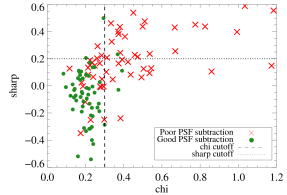
Figure 2.— chi/sharp isolation criteria. Visually identified blends (red crosses) and non-blends (green circles) are shown from a small representative area close to the center of M31. We reject all sources with DAOPHOT goodness-of-fit parameters chi > 0.3 (to the right of the dashed line) or shape parameter sharp > 0.2 (above the dotted line). The chi cutoff value is lowered in less dense fields farther from the galactic center.

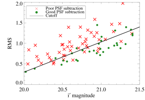
Figure 3.— RMS isolation criterion. Visually identified blends (red crosses) and non-blends (green circles) are shown from a small representative area about 8 kpc from the center of M31. The RMS deviation of the pixel values of the residual image in a $5\times 5$ pixel square centered on each source is plotted against the $i^{\prime}$ magnitude of the source. We reject all sources above the solid black line.

2.4. Observations

All slitmasks are observed using Keck/DEIMOS with the 1200 line mm^-1 grating. This configuration yields a spatial scale of $0\farcs 12$ pixel^-1 and a spectral dispersion of $0.33$ Å pixel^-1. We set the central wavelength to $7800$ Å, corresponding to a wavelength range of $\sim 6450-9150$ Å. The exact wavelength range for each slit varies as a result of location on the slitmask and/or truncation due to vignetting. The wavelength region is chosen to target the Ca II triplet absorption feature present in RGB stars. The anamorphic distortion factor for this grating and central wavelength is 0.606. Therefore, each $0\farcs 8$ wide slitlet subtends $4.1$ pixels. Better still, excellent seeing conditions ($\sim 0\farcs 6$) during observations can provide somewhat better spectral resolution yielding an average resolution of $3.1$ pixels $=1.0$ Å.

Reliable spectra (those that yield secure velocities, as described in § 2.7), are obtained from 4465 of the 5263 slitlets. Approximately $30\%$ of the slitlets from slitmask M32_3 did not produce useful spectra due to a warp in the slitmask.

See Table 1 for information on the positions of the slitmasks and the number of useful spectra recovered from each one.

2.5. Data Reduction

The Keck/DEIMOS multiobject slitmasks are processed using the spec2d and spec1d software (version 1.1.4) developed by the DEEP Galaxy Redshift Survey team at the University of California, Berkeley (Davis et al., 2003). Briefly, the reduction pipeline rectifies, flat-field and fringe corrects, wavelength calibrates, sky subtracts, and cosmic ray cleans the two-dimensional spectra, and extracts the one-dimensional spectra. For more details, see Howley et al. (2012).

2.6. Cross-Correlation Analysis

Line-of-sight (LOS) velocities for resolved targets are measured from the one-dimensional spectra using a Geha et al. (2010) modified version of the visual inspection software zspec, developed by D. Madgwick for the DEEP Galaxy Redshift Survey at the University of California, Berkeley. The software determines the best-fit LOS velocity for a target by cross-correlating its one-dimensional science spectrum with high signal-to-noise stellar templates in pixel space and locating the best fit in reduced-$\chi^{2}$ space.

A-band telluric corrections and heliocentric corrections are calculated and applied to the measured LOS velocities. The A-band telluric corrections, which account for velocity errors associated with the slight mis-centering of a star in a slit, are determined using the method discussed in Sohn et al. (2007) and Simon & Geha (2007).

LOS velocity errors are determined for each star by adding in quadrature the cross-correlation based velocity error and a systematic error estimated by repeat observations, as described in Howley et al. (2012). The typical LOS velocity error in our sample is 4–5 km s^-1.

2.7. Quality Assessment

Each two-dimensional spectrum, one-dimensional spectrum, and corresponding Doppler shifted template match are visually inspected in zspec and assigned a quality code based on the reliability of the fit. This process allows the user to evaluate the quality of a spectrum and reject instrumental failures and poor quality spectra. Velocity measurements based on two or more strong spectral features are labeled “secure.” Velocity measurements based on one strong feature plus additional marginal features are labeled “marginal.” Spectra that contain no strong features, low S/N and/or instrumental failures are considered unreliable, and so are not included in our analysis. Additional details on quality code assignment can be found in Guhathakurta et al. (2006). During this process, we also identify and flag $43$ likely MW M dwarfs based on their strong surface-gravity sensitive Na I 8190A doublet. These are excluded from the radial velocity analysis.

2.8. Serendipitous Sources

Upon visual inspection of the one-dimensional and two-dimensional spectra during the quality assessment phase outlined in § 2.7, some fraction of the slits clearly show that the slitlet intersects more than one star: the target star and one or more serendipitously detected stars, or serendips. Serendips are detected via one of two methods: through continuum detections that are offset from the primary target in the spatial direction, or by the detection of spectral features that are offset from the primary target in the spectral direction. Serendip detections occur frequently in the inner parts of M31 and close to M32 due to the severe crowding and blending in the CFHT/MegaCam data. Serendips are also assigned quality codes and those with secure or marginal velocities are included in the radial velocity analysis. More information on serendipitous detections can be found in Howley et al. (2012).

3. DATA ANALYSIS

We perform our analysis in each of the five spatial regions labeled in Figure 4. These regions are the SE minor axis (not expected to yield constraints on the spheroid rotation velocity); the SSW quadrant (expected to yield a constraint on the rotation velocity via a negative velocity offset from the systemic velocity of M31); and three regions along the northeast major axis, which we name NE1, NE2 and NE3 in order of increasing projected radial distance (expected to yield three independent estimates of the rotation velocity via positive velocity offsets from the systemic velocity of M31). Note that these regions are defined by lines of constant position angle and projected radius, and are not quite the same as the three data sets shown in Figure 1. The positions of and number of stars within each region are given in the first six columns of Table 2.

The kinematically cold peak at around $-100~{}\rm km~{}s^{-1}$ in Figure 5 suggests that our measured velocity distribution has a significant contribution from the disk. Hence, it is imperative that we realistically account for disk contributions. Instead of adopting a specific model for its velocity field, we only assume that the stellar disk is locally cold with a symmetric velocity distribution. As explained in § 3.1, we apply this assumption to divide each region into several subregions. To each subregion we fit two Gaussian distributions, corresponding to a kinematically cold and a hot component, where the hot component is required to have the same mean velocity and velocity dispersion across all subregions in a region (described in § 3.2). Lastly, in § 3.3 we describe how we modify our analysis to account for the possibility of contamination by the GSS and associated tidal debris.

3.1. Choice of Subregions and Expected Disk LOS Velocity Pattern

Because we assume that the disk is only locally cold, we fit for the disk in each of many small subregions. The spatial boundaries of individual subregions are dictated by two competing desirable factors, namely a small spread in disk mean velocity and high number statistics. Our assumption of a perfectly cold disk is only strictly true in the limit of infinitely small subregions. On the other hand, a multi-Gaussian fit to a velocity distribution requires a somewhat large number of points. We arbitrarily decide that $100$ is the minimum satisfactory number of points.

To estimate the spread of the mean disk velocity as a function of position, we employ a simple geometrical model for the rotation pattern of an inclined disk with perfectly circular motion (Guhathakurta et al., 1988):

$$v_{\rm obs}(\xi,\eta)=v_{\rm sys}\pm\frac{v_{\rm rot}(r_{\rm deproj})\sin(i)}{\sqrt{1+\tan^{2}(\Delta{\rm PA})/\cos^{2}(i)}}$$ (3)

where $\xi,\eta$ are tangent-plane coordinates with origin at the center of M31, $i=77^{\circ}$ is the inclination of the disk of M31, $v_{\rm sys}=-300\rm~{}km~{}s^{-1}$ is the systemic heliocentric velocity of M31, $\Delta\rm PA$ is the position angle projected onto the plane of the sky measured relative to the major axis of the disk of M31, $r_{\rm deproj}$ is the radial position measured in the plane of the disk, $v_{\rm rot}$ is the disk rotation speed, and the $+$ and $-$ signs apply to the NE and SW halves of the disk, respectively. An azimuthally averaged estimate for $v_{\rm rot}(r_{\rm deproj})$, based on HI kinematics, ranges from $\sim 250~{}\rm km~{}s^{-1}$ at $r_{\rm deproj}=15~{}\rm kpc$ to $\sim 175\rm~{}km~{}s^{-1}$ at $5\rm~{}kpc$ (Corbelli et al., 2010). The expected velocity spread calculated in this way will not be exact, because in addition to $\Delta\rm PA$, the true spread in mean stellar velocity over a subregion is influenced by $\Delta r_{\rm deproj}$ of the subregion, any departure from perfectly circular motion, and the intrinsic local velocity distribution (due to a multiple-component disk, for example).

Using Equation 3 with $v_{\rm rot}=250\rm~{}km~{}s^{-1}$, we bin our data in each region into subregions based on position angle. The angle subtended by a single subregion is approximately the greater of two $\Delta\rm PA$ criteria: 1) the $\Delta\rm PA$ such that the change in $v_{\rm obs}$ over a subregion due to $\Delta\rm PA$ is $10\rm~{}km~{}s^{-1}$, or 2) the $\Delta\rm PA$ that includes 100 data points. Our final subregions are shown in Figure 4. In the NE1–NE3 and SSW regions, we identify these subregions with subscripts that increase with distance from the nearest major axis: $\rm NE1_{1},NE1_{2},\ldots,NE1_{7};~{}SSW_{1},\ldots,SSW_{5},etc.$ In the SE region, the outer, inner south, and inner north subregions are named $\rm SE_{1},SE_{2},SE_{3},$ respectively. Note that we use this rotation pattern only to estimate appropriate bin sizes, not to determine disk rotation speeds. The final positions of and number of stars in each subregion are presented in the first six columns of Table 4 in the Appendix.

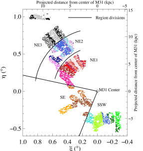
Figure 4.— Division into regions and subregions. Each point corresponds to a single velocity measurement. Solid lines delineate the five regions for which we obtain independent kinematical parameters of the spheroid: inner northeastern (NE1), intermediate northeastern (NE2), outer northeastern (NE3), southeastern (SE), and south-southwestern (SSW). Colors show the subregions within each region that are used to determine the disk contribution to the velocity distribution. With the exception of the SE region, our subregion naming convention is based on distance from the major axis. For example, in the NE3 region, $\rm NE3_{1}$ (light gray) straddles the major axis, $\rm NE3_{2}$ (black) is slightly farther out, and $\rm NE3_{3}$ (dark gray) is farthest from the major axis. In the SE region, we use projected distance from the center of M31 in addition to lines of constant position angle to define three subregions: $\rm SE_{1}$ (outer, yellow), $\rm SE1_{2}$ (inner south, dark brown) and $\rm SE1_{3}$ (inner north, light brown).

Figure 5.— Distribution of heliocentric radial velocities for all 3697 stars with reliable velocity measurements from the MCT slitmasks. The peak around $-$100$~{}\rm km~{}s^{-1}$ corresponds to the disk, the LOS projection of whose rotation speed causes stars to be offset by as much as $+$200$~{}\rm km~{}s^{-1}$ with respect to the $-$300$~{}\rm km~{}s^{-1}$ systemic velocity of M31 (dotted line).

3.2. Fitting the Velocity Distribution Model

We use a Markov chain Monte Carlo (MCMC) sampler to find the velocity distributions of the disk and spheroid in each region. The spheroid is modeled as a single Gaussian distribution for each region, while the disk is modeled as a Gaussian distribution for each subregion. The model likelihood at each point in parameter space is then:

(5)

where $N$ is the number of stars in our data set, and star $j$ with measured velocity $v_{j}$ is found in region $r(j)$ and subregion $s(j)$. The notation $\mathcal{N}\!\left(x\,\big{|}\,\mu,\,\sigma\right)$ indicates the Gaussian distribution with mean $\mu$ and standard deviation $\sigma$ evaluated at $x$. The scalar $f_{s}$, subject to $0\leq f_{s}\leq 1$, is the fraction of the stars in subregion $s$ that belong to the spheroid. The spheroid in region $r$ has mean velocity $\overline{v}_{\text{sph},r}$ and velocity dispersion $\sigma_{\text{sph},r}$, while the disk in subregion $s$ is characterized by velocity $\overline{v}_{\text{disk},s}$ and dispersion $\sigma_{\text{disk},s}$.

Subregion $\textrm{SSW}_{4}$ includes stars from the galaxy M32, so for that subregion only we replace the single-Gaussian disk model $\mathcal{N}\!\left(v_{j}\,\big{|}\,\overline{v}_{\text{disk},s(j)},\,\sigma_{\text{disk},s(j)}\right)$ with a double-Gaussian model.

The likelihood in Equation 5 can be sampled independently in each of the five regions. We use the code emcee (Foreman-Mackey et al., 2012), which implements the affine-invariant ensemble sampler of Goodman & Weare (2010), to perform the MCMC algorithm. In addition to the likelihood above, we must specify prior probability distributions for the parameters. For $f_{s}$ we use a uniform distribution on the interval $[0,1]$; for the mean velocities $\overline{v}_{\text{sph},r}$ and $\overline{v}_{\text{disk},s}$ we use flat priors; and for the dispersions $\sigma_{\text{sph},r}$ and $\sigma_{\text{disk},s}$ we demand positive values. If we sample each region independently, then the parameter space for region $r$ includes $\overline{v}_{\text{sph},r}$, $\sigma_{\text{sph},r}$, plus the set of $f_{s}$, $\overline{v}_{\text{disk},s}$, $\sigma_{\text{disk},s}$ for each subregion $s$ within $r$. We initialize the MCMC at $\overline{v}_{\text{sph},r}=-300\rm~{}km~{}s^{-1}$, $\sigma_{\text{sph},r}=150\rm~{}km~{}s^{-1}$, each $f_{s}=\frac{1}{2}$, and $\overline{v}_{\text{disk},s}$ and $\sigma_{\text{disk},s}$ = the sample mean and standard deviation of the velocities in subregion $s$.

Briefly, the MCMC ensemble sampler works as follows. It explores the parameter space by maintaining a set of walkers. Each walker represents a point in the parameter space. At each iteration of the MCMC, each walker takes a step in the parameter space by choosing another walker and stepping along the line in parameter space connecting itself to the other walker. The step size is chosen stochastically and allows interpolation as well as extrapolaton. In effect, the walkers choose their steps based on the covariance of the set of walkers. After each step is taken, the posterior probability distribution at the new point in parameter space is evaluated. Steps that increase the probability are always accepted, while steps that decrease the probability are sometimes accepted. After a large number of steps, the ensemble of walkers will sample the parameter space with frequency proportional to the posterior probability distribution; we can draw fair samples from the distribution by selecting points from the histories of the walkers. We estimate the mean and variance of each parameter (assuming unimodal distributions) based on sample statistics of the histories of the walkers. In particular, we allow each of 32 walkers to take 10,000 steps. We then compute the mean spheroid velocity as the mean value of $\overline{v}_{\text{sph},r}$ over the last 2000 steps of all the walkers (i.e., the mean of 64,000 points), and the 68% confidence interval as the standard deviation of that quantity over the last 2000 steps of all of the walkers. We use the same method to estimate the values and uncertainties of the spheroid dispersion and the disk parameters. We report these values in columns 7 and 8 of Table 2 and illustrate them in Figure 9.

3.3. Accounting for Tidal Debris Associated with the Giant Southern Stream

The analysis described thus far separates the spheroid from the disk (and from M32 in subregion $\text{SSW}_{4}$). The mean velocity and dispersion we extract describe the average properties of the spheroid, regardless of its underlying structure.

Several lines of evidence, however, suggest that our measurements do not well represent a rotation curve of a smooth spheroid. First, the mean spheroid velocities in the five regions do not follow a physical rotation pattern: the mean velocity of the NE2 region is consistent with zero, while the surrounding regions (NE1 and NE3) are rotating at about $50~{}\rm km~{}s^{-1}$ in the same direction as the disk. Second, the sum of hot and cold Gaussians does not well represent the velocity distributions. A chi-squared analysis applied to the data binned by $20~{}\rm km~{}s^{-1}$ reveals that that the probability of the model representing the velocity distribution is relatively low (see the final column of Table 2).

Velocity histograms, such as those in Figure 6, suggest that cold substructure, possibly tidal debris from the GSS, could be skewing our measurements. A close-up view of the negative-velocity tail of the NE2 histogram reveals a cold spike of about 10 stars in excess of the Gaussian tail at $-580\rm~{}km~{}s^{-1}$ (Figure 6, top right). A slight overdensity of points at this velocity can be seen in the NE1 and NE3 histograms as well. Though nothing is immediately visible in the SE or SSW regions, a few extra stars around $-580~{}\rm km~{}s^{-1}$ would be partially concealed by the bulk of the velocity distribution.

Figure 7 shows another projection of these data: the velocity of each star in the NE1, NE2, and NE3 regions plotted against $R_{\rm proj}$. Also shown (in turquoise triangles) are data from two GSS fields at 17 and 21 kpc (Gilbert et al., 2009). The concentrations of stars at approximately $-500$ and $-400~{}\rm km~{}s^{-1}$ in these data represent the GSS and the secondary stream, respectively. The magnitudes of the central stream velocities increase with decreasing $R_{\rm proj}$ as the streams fall into the potential well of M31 from the south. The black crosses in Figure 7 show the expected stream velocity as a function of radius closer to the center of M31 (Fardal et al., 2012). The NE region data from this work show clear concentrations of objects near the predicted stream velocity, continuing the trend seen south of the galaxy. Hence, it seems unlikely that the peak in the Figure 6 histograms is simply a binning artifact, and probable that it comes from the northern extension of a cold tidal stream.

To account for the presence of the GSS and its associated tidal debris, we repeat the MCMC fits in regions NE1, NE2, NE3, and SSW after removing all stars within $\sigma=\pm 30\rm~{}km~{}s^{-1}$ of the predicted velocities of the two streams. (The measured velocity dispersion of the stream from Gilbert et al. (2009) is $20~{}\rm km~{}s^{-1}$; however, we use the larger value to ensure that we exclude all stream stars despite the slightly uncertain mean stream velocity.) In the SE minor axis region, we exclude all stars with velocity $v<-600~{}\rm km~{}s^{-1}$ or $v>0~{}\rm km~{}s^{-1}$. The former is to account for GSS debris, and the latter for SE Shelf stars (GSS debris from third pericentric passage) (Gilbert et al., 2007).

We account for the fact that we have removed stars within a range of velocities by renormalizing the Gaussian distributions. That is, given a Gaussian velocity distribution, we compute the fraction of the probability mass that falls within the excised velocity range and scale up the remainder of the distribution so that the integral over the remaining (unexcised) velocities is unity. The resulting kinematical spheroid parameters are reported in columns 7 and 8 of Table 3.

The resulting fit for region NE1 is plotted in Figure 8. The first seven panels show the seven subregions in NE1. In each panel, each walker at the end of 10,000 steps is represented by a set of colored lines: a red Gaussian with parameters $f_{s},~{}\overline{v}_{\text{sph},r},~{}\sigma_{\text{sph},r}$ and a blue or green Gaussian with parameters $(1-f_{s}),~{}\overline{v}_{\text{disk},s},~{}\sigma_{\text{disk},s}$. The sum of these two is shown in violet. These distributions are overlaid on the velocity histogram of stars in the subregion. The velocity ranges excised for stream debris are shown in two ways: the velocity range is shaded in light gray, and the stars in this range are colored red.

The bottom middle panel shows the cumulative best-fit distributions: the red line is the Gaussian corresponding to the mean $(\overline{v}_{\text{sph},r},~{}\sigma_{\text{sph},r})$. The blue curve is the cumulative disk distribution: the sum of the mean disk Gaussians from the seven subregions. The violet is the sum of the other two curves. The excised velocity ranges are respresented in the same way as in the subregion panels.

The bottom right panel shows the positions of the walkers in parameter space after 10,000 steps. There are eight concentrations of points corresponding to the eight $(\overline{v},~{}\sigma_{v})$ pairs (one spheroid and seven disk). Each pair is summarized by an ellipse displaying the mean and dispersion of that distribution.

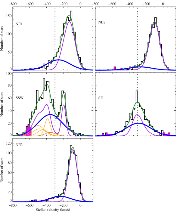
Figure 6.— Maximum likelihood fits of a kinematically hot spheroid to each of the five regions in our sample, after excluding the velocity range encompassing the GSS and its associated tidal debris (shaded pink). Violet lines show the cumulative region cold component; blue show the best-fit spheroid Gaussian; green show the sum of these two components. The dashed lines show the systemic velocity of M31 relative to the MW. Individual subregion cold components are shown in orange in the SSW region panel, but left out of the other panels for clarity. We remind the reader that our fitting procedure makes use of the distinct velocity profiles of the individual subregions as shown in Figures 8 and 13-16, so that the fits are much better constrained than may be apparent from the combined distributions here.

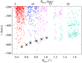
Figure 7.— Radial velocity vs. projected radius of the most negative-velocity stars in the NE1, NE2, and NE3 regions (red, blue, and magenta, respectively). Overplotted are data from two fields centered on the GSS south of M31 (turquoise triangles) (Gilbert et al., 2009). The clusters of these turquoise triangles around $v\sim-500~{}\rm km~{}s^{-1}$ and $v\sim-390~{}\rm km~{}s^{-1}$ are the GSS and the secondary stream, respectively. The black crosses show six points for the predicted velocity of the NE Shelf (Fardal et al., 2012). The GSS appears to be present in the NE fields as slight concentrations around the black crosses.

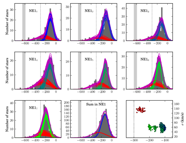
Figure 8.— MCMC fits of kinematically hot (red) and cold (blue to green) components to each of 7 subregions in the NE1 (inner northeast major axis) region plotted over velocity histograms of stars in each subregion. Subregions progress from $\rm NE1_{1},$ straddling the NE major axis, to $\rm NE1_{7},$ farthest from the major axis. One curve is drawn for each component for each of the 32 walkers in the MCMC. Each violet distribution is the sum of the hot and cold distributions corresponding to a single walker. Velocity ranges excluded due to possible contamination by tidal debris from the GSS are shown in two ways: by the gray shaded regions, and by the stars shaded red on the histogram. The bottom middle panel shows the best-fit hot component (red) that, when added to the cumulative region cold distribution (blue), best fits the observed velocity distribution. The bottom right panel shows the final position of the walkers in parameter space. Ellipses show the mean and uncertainty of each of the parameters $(\overline{v},\sigma_{v})$ for each of the kinematical subcomponents. The dotted line in each panel marks the systemic velocity of M31 relative to the MW.

4. DISCUSSION

This section is organized as follows. We first present the rotation curve and velocity dispersion profile for the inner spheroid in § 4.1. In §  4.2 we compare the velocity dispersion of the cold component to previous measurements of the stellar disk as a sanity check on our analysis method. In § 4.3 we show that the exclusion of velocity ranges corresponding to tidal debris from the GSS significantly impacts the measured kinematical parameters of the spheroid, but has minimal effect on the cold component. In § 4.4 we compute a spheroid membership probability for each star in our sample. In § 4.5 we explain that the spheroid is likely supported by velocity anisotropy in addition to rotation. Finally, in § 4.6 we show that neither spectroscopic target selection criteria nor degree of crowding introduces a significant bias towards the kinematically cold or hot population.

4.1. Kinematical Parameters of the Inner Spheroid

The spheroid distributions corresponding to the best-fit $\overline{v}_{\rm sph}$ and $\sigma_{\rm sph}$ (hereafter $\sigma_{v}$) are plotted in Figure 6 for each of the five regions. (This figure is simply a compilation of the summary panels of Figures 8 and 13–16.) Kinematical and goodness-of-fit parameters, accounting for the GSS and associated tidal debris, are reported in Table 3. The $\chi^{2}$ probabilities have improved significantly from the uncorrected values in Table 2. Four of the five regions now have probabilities greater than 90%, and that of the fifth (SSW) has increased by a factor of 15.

The dispersion profile is shown in the right panel of Figure 10. The profile appears to decrease smoothly with radius, though it is consistent with flat to $2\sigma$. The best-fit line to this profile is

$$\sigma_{v}(a_{\rm eff})=(159.5\pm 10.8)-(2.9\pm 1.3)\frac{a_{\rm eff}}{1~{}\rm kpc}~{}\rm km~{}s^{-1}.$$ (6)

where $a_{\rm eff}$ is the effective spheroid major axis coordinate, assuming a 5:3 axis ratio (Pritchet & van den Bergh, 1994). Our dispersion profile is consistent with that measured by Gilbert et al. (2007) but is slightly offset from other existing measurements, including the Saglia et al. (2010) integrated-light measurement at 1.1 kpc on the major axis of the bulge (black square in Figure 10) and the linear dispersion profile of Chapman et al. (2006). These differences should be taken lightly, though, because the measurements are not directly comparable. The Saglia et al. (2010) point may be slightly deflated by contributions from the low-dispersion disk stars, which those authors estimate contribute about $30\%$ of the light in the slit. The Chapman et al. (2006) profile, meanwhile, is the innermost limit of measurements primarily made farther out in the halo, so we do not necessarily expect agreement at the radii covered by our study.

We also compare our results to the dispersion profile produced by a model with spherical, isotropic, non-rotating bulge and halo stellar components as well as a stellar disk and halo ($M/L=2.5$) and bulge ($M/L=5.6$) (dotted orange line in Figure 10; Fardal et al., 2012). The model falls below our data at the $2\sigma$ level in the NE2 and NE3 regions and at the $3\sigma$ level in the SE and NE1 regions. The mismatch suggests that, for example, the mass profile of the model galaxy is too shallow, or the gradient of the density profile of the tracer population is too large. A more detailed analysis is beyond the scope of this paper.

Extracting the intrinsic rotation curve of the spheroid is nontrivial. The relationship between the mean LOS velocity and the intrinsic rotation velocity depends on the orbital dynamics of the spheroid, and in general is difficult to determine without detailed 2D or 3D kinematical mapping. Therefore, in the left panel of Figure 10 we simply present the mean LOS component of the velocity versus the effective major axis coordinate (based on a 5:3 axis ratio). Though two points are consistent with zero to $2\sigma$, we detect significant rotation in the SSW, NE1 and NE3 regions. The average value of $|v-v_{\rm M31}|$, excluding the SE minor axis point, is $52.6\pm 6.8~{}\rm km~{}s^{-1}$ (solid line in Figure 10). All four off-minor axis points are consistent with this mean velocity to better than $1\sigma$. This is the first measurement of significant rotation in the inner spheroid.

The velocity dispersion of M31’s inner spheroid is similar to that the halo of the MW at similar radii, but its mean velocity is significantly larger. The velocity ellipsoid of the MW’s inner halo is $(\sigma_{V_{R}},\sigma_{V_{\phi}},\sigma_{V_{Z}})=(150\pm 2,95\pm 2,85\pm 1)$ (Carollo et al., 2010), on the same order as the LOS component of the M31 spheroid dispersion. However, the MW’s inner halo has a mean rotation velocity consistent with zero (Carollo et al., 2010).

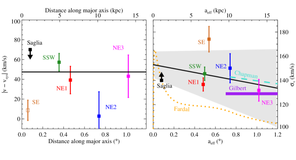
Figure 9.— Velocity (left) and dispersion (right) profiles for M31’s inner spheroid without accounting for the GSS or associated tidal debris. Left: Mean velocity is plotted against the projection along the major axis coordinate. The SE minor axis (brown open square) is close to the minor axis, so we do not expect to measure a significant ${|\overline{v}-v_{\rm sys}|}$ due to rotation. The black line in the left-hand plot is the mean value of the four off-minor-axis velocity measurements. Right: Dispersion is plotted versus $a_{\rm eff}$, the effective major axis coordinate for a spheroid with a 5:3 axis ratio. The best fit line to our dispersion measurements is shown by the solid black line, with the region within $\pm~{}1\sigma$ of the best-fit line shaded in gray. Also plotted are limits on the bulge mean rotation velocity and velocity dispersion from Saglia et al. (2010, black points with arrows), and velocity dispersion measurements further out in the spheroid by Chapman et al. (2006) and Gilbert et al. (2007, horizontal purple line). The orange dotted line represents a model dispersion profile that includes isotropic bulge and halo stellar components, as well as a stellar disk and dark matter halo (Fardal et al., 2012).

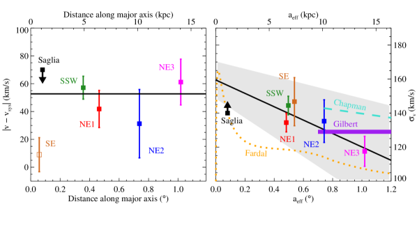
Figure 10.— Same as Figure 9, excluding stars in the velocity ranges corresponding to the GSS and associated tidal debris.

4.2. Dispersion and Velocity of the Cold Population

The cold component $(\overline{v},\sigma_{v})$ for each subregion are plotted against $r_{\rm deproj}$ in Figure 17. As a sanity check on our analysis method of fitting multiple Gaussians to subregions, we compare these values to previously measured kinematical parameters of the stellar disk. The cold component in a single subregion has an average dispersion of $58\rm~{}km~{}s^{-1}$, reasonably consistent with the Collins et al. (2011) dispersion measurements of $51~{}\rm km~{}s^{-1}$ and $36~{}\rm km~{}s^{-1}$ for the thick and thin stellar disks, respectively. We expect our dispersion to be larger than the local value, primarily because the finite spatial extent of our subregions necessarily smears out the velocity distribution. For example, if the spread in mean velocity due to $\Delta PA$ is $\sim\!\!20~{}\rm km~{}s^{-1}$ in a subregion, and the true velocity dispersion is $~{}\sim\!\!40~{}\rm km~{}s^{-1}$, then we would expect to measure an effective dispersion of $\sqrt{20^{2}+40^{2}}=45~{}\rm km~{}s^{-1}.$ This effect is accentuated if there is an additional spread in mean velocity with radius. Therefore, the fact that our cold component looks like the thick disk of Collins et al. (2011) does not imply that the thick component dominates the stellar disk.

A possible concern is that contributions from multiple stellar disk components (a combination of thin, thick, or extended) may invalidate our assumption of a locally cold disk. If this were the case, we would expect to see non-Gaussianity in the velocity signature of the cold component. However, Table 4 shows that that the velocity distributions of the cold components in most of the subregions are well fit by a single Gaussian. While this observation does not say anything about the kinematical structure of the disk, it does suggest that our simple assumption is adequate for our purpose of describing the spheroid.

It is also possible that a kinematically warm thick disk component would be incorporated into our Gaussian representation of the spheroid; however, the high goodness-of-fit statistic again suggests that this is not a significant effect. In any case, the bias on our kinematical spheroid parameters induced by thick disk contamination confirms, rather than invalidates, our qualitative results, as discussed in § 4.5.

A closer look at the best-fit cold and hot components by subregion in Figures 8 and 13–16 show that the trends in the cold component with position angle match those expected for an inclined rotating disk. For example, in Figure 8, the mean velocity of the cold component (blue and green curves) transitions from $-100~{}\rm km~{}s^{-1}$ in subregion $\rm NE1_{1}$, along the major axis, to $-200~{}\rm km~{}s^{-1}$ in subregion $\rm NE1_{7}$, farthest from the major axis. In other words, the absolute value of the offset of the mean velocity of the cold component from the systemic velocity of M31 moves closer to zero as we march away from the major axis. This progression is clear in Figures 13 and 14 for regions NE2 and NE3 as well, although it is less pronounced because these regions subtend a smaller range in PA.

4.3. Effect of Tidal Debris Associated with the GSS on Spheroid Kinematics

Accounting for the GSS and its associated debris has a significant effect on the measured kinematical parameters of the underlying smooth inner spheroid, supporting the observation of Fardal et al. (2007) that the debris was visible in the samples of Ibata et al. (2005), Chapman et al. (2006), and Merrett et al. (2006).

It is unclear whether the secondary stream identified by Kalirai et al. (2006b) and confirmed by Gilbert et al. (2009) is present in the NE1–NE3 regions. Figure 7 reveals a second clump of objects in the NE2 region, offset from the primary stream by 75–100$~{}\rm km~{}s^{-1}$, the same separation as that between the two streams south of the galaxy. However, such clumps are barely, if at all, visible in the NE1 and NE3 regions, and their exclusion does not significantly affect the kinematical parameters of the spheroid. Further observations are necessary to determine if there is a second substructure and, if so, whether it has a physical connection to the GSS.

Is the GSS the only source of nonvirialized substructure biasing our measurements of the mean velocity and dispersion of the inner spheroid? While we cannot prove that all stars except those in the excised velocity ranges belong to either a disk or a perfectly smooth spheroid, we can show that the effect of other nonvirialized substructure on our kinematical characterization of the underlying smooth spheriod is negligible. In star-count maps of the inner regions of M31, such as those in Ibata et al. (2001), the GSS is by far the most prominent substructure. Even so, GSS stars account for only a small fraction of our spectroscopic sample (see pink shaded regions in Figure 6), and have a relatively small effect on our results. Other, less-prominent substructures would (1) be nearly impossible to detect and account for, and (2) have a negligible effect on the measured kinematical parameters of the inner spheroid.

4.4. Spheroid/Disk Membership Probability and Extreme Velocity Stars

We can apply our subregion fits to quantify the spheroid membership probability for any star. At the location and velocity of each star in our sample, we calculate the ratio of the values of the best-fit hot component in that region and the disk and M32 components in that subregion. The disk and M32 membership likelihoods are calculated in a similar fashion. The results are sorted into three categories as follows: stars that are at least three times as likely to be disk members as anything else (yellow in Figure 11); stars at least three times as likely to be spheroid members as anything else (magenta); and other objects, including likely M32 members (green). As expected, objects on the major axis are much more likely to be disk members than are those on the minor axis. Most important, we see likely spheroid members at all radii covered by our sample.

Recently, Caldwell et al. (2010) reported discovery of an “extreme velocity” star at a projected radius of $4$ kpc ($0.3^{\circ}$) along the SW major axis of M31. The star has a velocity of $-780~{}\rm km~{}s^{-1}$, essentially excluding it from membership in the thin, cold stellar disk. Those authors attribute the star’s highly negative velocity to possible membership in the GSS, even though it would have to be a $6\sigma$ outlier of the stream velocity distribution. Our probability map demonstrates that this object can more easily be interpreted as a member of the spheroid, even at these large radii: it may be a $4\sigma$ outlier of the spheroid distribution.

It is tempting to interpret this distribution of probabilities as a map of bulge-to-disk fraction. However, this statistic can be more reliably constrained using photometric light-profile fitting in conjunction with kinematical decomposition. This study will be presented in Dorman et al. (2012, in prep).

Figure 11.— Probable subcomponent membership of each star based on location and velocity. Stars at least 3 times more likely to be a disk member than anything else are shown in yellow; those at least 3 times more likely than anything else to be a spheroid member are shown in pink; all other objects, including likely M32 members, are shown in green. Region divisions are shown as solid lines.

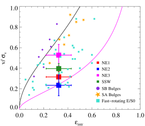
Figure 12.— Anisotropy diagram for spheroidal systems. The large filled squares show the ratio of the observed mean velocity and the velocity dispersion against the intrinsic ellipticity of M31’s spheroid. Error bars represent the range of reported ellipticities converted to edge-on intrinsic ellipticities as explained in Cappellari et al. (2007). The black curve shows the expected value of the ratio $\overline{v}/\sigma_{v}$ as a function of ellipticity for an isotropic, rotating galaxy. The magenta line approximates the behavior of an oblate anisotropic galaxy with anisotropy parameter $\delta\sim 0.7\epsilon$ (Cappellari et al., 2007). Also shown are fast-rotating E/S0 galaxies from SAURON (turquoise squares) and bulges of barred [violet circles, (Kormendy, 1982b)] and unbarred [orange stars, (Kormendy & Illingworth, 1982)] spirals. The inner spheroid of M31 appears to be flattened by velocity anisotropy in addition to rotation, and therefore more closely resembles an elliptical galaxy than a spiral galaxy bulge.

4.5. Anisotropy

We investigate the degree to which the flattening of the spheroid may be due to rotation by comparing the spheroid ellipticity $\epsilon=1-b/a$ to the ratio $v/\sigma_{v}$. The value of $\epsilon$ is uncertain at these radii. Pritchet & van den Bergh (1994) measure $\epsilon=0.4$ with limited data at $R_{\rm proj}=10~{}\rm kpc$. Courteau et al. (2011) perform a fit to a more extended data set to obtain values between $0.21$ and $0.37$, depending on their bulge/disk decomposition and modeling technique, for a relatively small bulge with scale length $\sim 1.0~{}\rm kpc$.

Despite this range of possible ellipticities, $\overline{v}/\sigma_{v}$ of the spheroid in every region is lower than that of a rotationally flattened oblate isotropic rotator (black line in Figure 12). We measure $\overline{v}/\sigma_{v}$ = 0.23–0.52, but $v_{\rm rot}/\sigma_{v}$ of $0.87$ or $0.54$ would be required for rotation to flatten the spheroid to an ellipticity of $0.4$ or $0.21$, respectively. Hence, rotation alone probably does not account for all of the flattening of the spheroid.

It is possible that anisotropy in the velocity ellipsoid can provide the remainder of the flattening. Anisotropy can be parameterized by

$$\delta\equiv 1-\frac{\Pi_{zz}}{\Pi_{xx}}$$ (7)

where $z$ points along the axis of symmetry of the spheroid, $x$ is any orthogonal direction (say, $r$), and $\Pi_{kk}$ represents the pressure from velocity dispersion along direction $k$ (e.g. Cappellari et al., 2007). In a system with an axisymmetric velocity ellipsoid, $\delta=0$ corresponds to a system whose flattening is unaffected by anisotropy, while $\delta\sim 1$ corresponds to a system whose flattening is almost entirely due to anisotropy. Using the iterative method described in Cappellari et al. (2007), we find that an anisotropy of $\delta=$ 0.05–0.27 is required to explain a spheroid ellipticity of 0.21–0.4, given the mean value of $\overline{v}/\sigma_{v}$ in regions NE1–NE3 and SSW.

We compare the inner spheroid of M31 to other spheroidal systems. The bulges of spiral galaxies generally fall on or above the line for rotationally-flattened systems (Kormendy & Illingworth, 1982; Kormendy, 1982b). In contrast, so-called “fast-rotating” ellipticals tend to lie between this line and the line $\delta\sim 0.7\epsilon_{\rm intr}$ (magenta in Figure 12) (Cappellari et al., 2007). However, these comparison systems are observed at around one effective radius $(r_{\rm eff})$, whereas our kinematical measurements range from 1.5–14$~{}r_{\rm eff}$. The inner spheroid of M31, then, more closely resembles the inner $r_{\rm eff}$ of a fast-rotating elliptical than the central bulge of a spiral galaxy.

As suggested earlier in § 4.2, it is possible that the spheroid velocity distribution may be contaminated by thick disk stars. If so, the true spheroid mean velocity is lower than we report, and the true spheroid dispersion higher. However, note that the $\overline{v}/\sigma_{v}$ of the spheroid is already small enough to look more like an elliptical galaxy than the bulge of a spiral galaxy. The possible bias induced by a thick disk component would merely increase this effect, confirming our conclusion that M31’s inner spheroid rotates unusually slowly.

4.6. Effect of Target Selection Criteria on Velocity Distribution

The majority of our spectroscopic targets were chosen on the basis of $i^{\prime}$ magnitude only, but a small fraction of the targets in the MCT region were identified based on position in the PHAT CMD. This latter category contains proportionally more of the rarer metal-poor and metal-intermediate RGB populations. If metal-poor and metal-intermediate RGBs preferentially trace the kinematically hot population, then inclusion of the PHAT-selected objects could bias our measurements, especially our spheroid membership probabilities. To test for bias, we performed a Komolgorov-Smirnov (K-S) test comparing the velocity distributions of the PHAT-selected targets and the magnitude-selected targets in each subregion. The test confirmed that the two distributions were indistinguishable.

Similarly, we used a K-S test to confirm that inclusion of crowded objects does not bias us towards one structural subcomponent. We created two lists of objects: “crowded” (those sharing a slit with at least one serendipitously detected neighbor) and “isolated” (those without any such neighbors). Again, there was no singificant difference between the velocity distributions of the two categories in any subregion.

Table 2Uncorrected Kinematical Spheroid Parameters

Region	$\xi~{}(^{\circ})$	$\eta~{}(^{\circ})$	$R_{\rm proj}$ (kpc)	$a_{\rm eff}$ (kpc)	$N_{\rm region}$	$\overline{v}-\overline{v}_{M31}~{}(\rm km~{}s^{-1})$	$\sigma_{v}~{}(\rm km~{}s^{-1})$	$N_{\rm spheroid}/N_{\rm total}$	$\chi^{2}$ prob
NE1	0.40	0.31	6.45	6.81	1615	$+$39.3 $\pm$ 13.9	136.7 $\pm$  5.4	0.288	0.731
NE2	0.48	0.55	10.11	10.31	1180	$+$2.8 $\pm$ 24.6	150.1 $\pm$ 12.0	0.120	0.136
NE3	0.64	0.79	13.93	14.00	859	$+$48.0 $\pm$ 24.0	131.4 $\pm$ 9.9	0.203	0.930
SE	0.26	$-$0.14	4.30	6.91	684	$+$8.7 $\pm$ 10.3	174.1 $\pm$  10.5	0.522	0.121
SSW	$-$0.09	$-$0.40	5.69	6.73	1313	$-$57.3 $\pm$ 8.9	145.5 $\pm$  5.5	0.465	1.5$\times 10^{-5}$

Table 3Kinematical Spheroid Parameters Corrected for Tidal Debris

Region	$\eta~{}(^{\circ})$	$\xi~{}(^{\circ})$	$R_{\rm proj}$ (kpc)	$a_{\rm eff}$ (kpc)	$N_{\rm region}$	$\overline{v}-\overline{v}_{M31}~{}(\rm km~{}s^{-1})$	$\sigma_{v}~{}(\rm km~{}s^{-1})$	$N_{\rm spheroid}/N_{\rm total}$	$\chi^{2}$ prob
NE1	0.40	0.31	6.45	6.81	1615	$+$41.8 $\pm$ 13.3	134.4 $\pm$  5.5	0.297	0.945
NE2	0.48	0.55	10.11	10.31	1180	$+$31.3 $\pm$ 24.5	135.3 $\pm$ 12.5	0.130	1.000
NE3	0.64	0.79	13.93	14.00	859	$+$61.2 $\pm$ 16.44	117.5 $\pm$ 8.8	0.198	0.998
SE	0.26	$-$0.14	4.30	6.91	684	$+$9.0 $\pm$ 12.2	144.5 $\pm$  5.5	0.571	0.819
SSW	$-$0.09	$-$0.40	5.69	6.73	1313	$-$57.1 $\pm$ 8.2	145.4 $\pm$  6.5	0.484	2.1$\times 10^{-4}$

5. SUMMARY & CONCLUSIONS

We have measured reliable radial velocities of over five thousand red giant branch stars in the inner $20\rm~{}kpc$ of M31 using the Keck/DEIMOS multiobject spectrograph. Targets were selected using a series of statistical tests designed to identify isolated M31 members bright enough to yield quality spectra.

By fitting a locally cold disk and a kinematically hot spheroid to the velocity distribution with an MCMC algorithm, we have measured the most probable kinematical parameters $\overline{v}$ and $\sigma_{v}$ of the red giant stellar population of the inner spheroid of M31 in each of five spatial bins. We find that, though the raw values are inconsistent with a physical rotation pattern, accounting for the presence of tidal debris due to the GSS allows us to detect a significant spheroid rotation velocity.

We find that probable spheroid members are present at all radii in our sample. When used in conjunction with integrated-light measurements, these membership probabilities will be a powerful tool for rigorous bulge/disk decomposition in the inner parts of M31.

We also compare the $\overline{v}/\sigma_{v}$ of the inner spheroid to those of other spheroidal structures. We find that rotation is insufficient to explain the flattening of the inner spheroid; it more closely resembles an anisotropic fast-rotating elliptical than the bulge of a spiral or barred spiral galaxy as measured at $\sim 1~{}r_{\rm eff}$.

Our magnitude-limited survey biases us towards the bright, old stellar population. As more PHAT data becomes available over the next few years, we will be able to select spectroscopic targets that represent a range of stellar populations within our magnitude range. We plan to present an analysis of the kinematics of different stellar populations in an upcoming paper.

6. Acknowledgments

We would like to thank the referee Alan McConnachie for helpful comments and Roeland van der Marel and Elisa Toloba for useful discussions.

PG, KH, MF and CD acknowledge NSF grants AST-0607852 and AST-1010039. PG, KH and CD acknowledge NASA grant HST-GO-12055. Additionally, CD was supported by a University of California Eugene Cota-Robles Graduate Fellowship and a NSF Graduate Research Fellowship.

We wish to recognize and acknowledge the very significant cultural role and reverence that the summit of Mauna Kea has always had within the indigenous Hawaiian community. We are most fortunate to have the opportunity to conduct observations from this mountain.

Appendix A MCMC results for regions NE2, NE3, SE, and SSW

Figures 13–16 are the analogs of Figure 8 for regions NE2, NE3, SE, and SSW, respectively. In this appendix, we briefly describe the results in each of these regions.

A.1. NE2 Region

Eleven stars are excluded from the MCMC fit in the NE2 region due to possible tidal debris membership; as seen in Figure 13, all are from the four subregions closest to the major axis. Exclusion drastically improves the chi-squared probability that the spheroid plus disk Gaussians are a good representation of the velocity distribution, raising it from 0.136 to 1.000. Exclusion also increases the mean velocity and decreases the velocity dispersion of the spheroid, bringing them much more into agreement with those measured in the other regions.

Several trends characterize the subregion panels. First, the fraction of stars in the spheroid (parameterized by ratio of the areas of the red spheroid and blue/green disk curves) increases with increasing distance from the major axis. Second, the mean velocity of the cold component decreases with increasing distance from the major axis. Reading off the velocity axis of the parameter-space view in the bottom right panel, we see that the mean velocity of the cold component moves from about $-90$ to $-170~{}\rm km~{}s^{-1}$. The minimum velocity is less negative than that in region NE1 because region NE2 subtends a smaller range in PA.

A.2. NE3 Region

Nine stars are excluded from region NE3 as possible tidal debris contaminants. Exclusion slightly improves the reduced chi-squared of the fit. It also slightly increases the mean velocity of the hot component and decreases the velocity dispersion, bringing them more into agreement with those measured in the other regions.

Because this region is centered farthest from the center of M31, it subtends the smallest range in PA of the three NE regions, and so the variation in cold component mean velocity between subregions is small. However, the parameter-space view in Figure 14 shows that the cold component kinematical parameters are very well defined.

A.3. SE Region

We exclude 36 stars from the tails of the velocity distribution in the SE minor axis region. While this does not skew the results of the MCMC fits in one direction or another, it does serve to increase the uncertainty in the final kinematical parameters; this effect can be seen in the large scatter in the walker positions in the parameter-space view in Figure 15.

The minor axis is a saddle point in the velocity field of M31. Here, the observed rotation velocity changes from less negative than $-300~{}\rm km~{}s^{-1}$ on the north side to more negative than $-300~{}\rm km~{}s^{-1}$ on the south side. The mean velocities of the cold component reflect this transition. The parameter-space view in the final panel of Figure 15 shows that in subregion $SE_{1}$ (blue), which lies parallel to and just north of the minor axis, we measure a mean velocity slightly less negative than the systemic velocity of M31. In subregions $SE_{2}$ (turquoise) and $SE_{3}$ (green), situated south and north of the minor axis, respectively, we measure mean velocities more negative and less negative than $-300~{}\rm km~{}s^{-1}$. Finally, we notice that the fraction of spheroid members is smallest in subregion $SE_{1}$, which is centered farthest from the center of the galaxy than the other two subregions.

A.4. SSW Region

Eleven stars fall into the velocity range excluded due to stream contamination in the SSW region. The exclusion does not have a significant effect on the mean velocity or dispersion of the hot component. The chi-squared probability of a good fit is lower in the SSW region than in the others, but exclusion of the possible stream stars improves the probability by a factor of about 15.

Subregion $\rm SSW_{4}$ completely contains the galaxy M32, which is treated as a second cold component. (In a previous trial run, we allowed for the possibility of a second cold component in each of the five subregions, but the best-fit fraction of M32 stars in subregions $\rm SSW_{1-3,5}$ was zero.) The parameter-space view in Figure 16 shows that the mean velocity and dispersion of M32 are very well constrained around $-200$ and $27~{}\rm km~{}s^{-1}$, respectively.

As in the NE regions, the fraction of stars in the spheroid is higher in the subregions farther from the major axis.

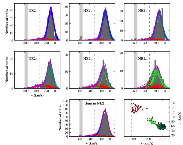
Figure 13.— Same as Figure 8, but for the NE2 region.

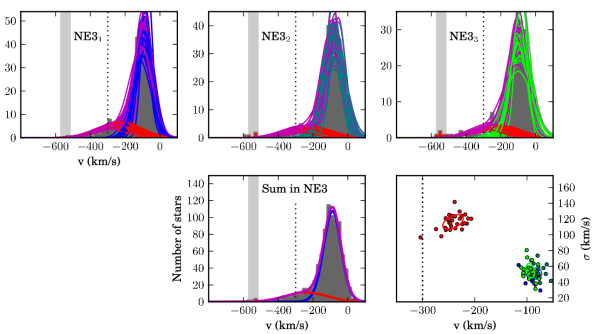
Figure 14.— Same as Figure 8, but for the NE3 region.

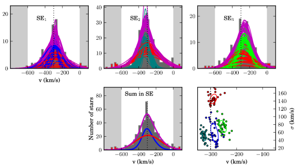
Figure 15.— Same as Figure 8, but for the SE region. $\rm SE_{1}$, $\rm SE_{2}$ and $\rm SE_{3}$ are the outer, inner south, and inner north subregions, respectively.

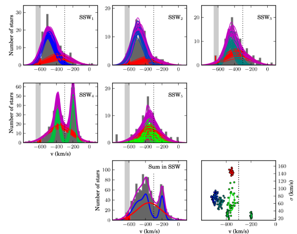
Figure 16.— Same as Figure 8, but for the SSW region.

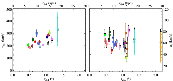
Figure 17.— Kinematical parameters of the cold component in each subregion, with $1\sigma$ error bars, before exclusion of velocity ranges corresponding to GSS debris (black points) and after exclusion (colored points). Note that exclusion of tidal debris has a negligible effect on the cold component. These cold components correspond to M31’s stellar disk. The left panel shows the rotation velocity of each cold component (computed using Equation 3) vs. the mean $r_{\rm deproj}$ of each subregion. The three SE subregions have been excluded because they do not yield meaningful constraints on the rotation velocity. The right panel shows the velocity dispersion. The velocity and dispersion follow the trends expected for M31’s stellar disk, supporting the idea that that our minimal assumption of a locally cold disk adequately accounts for disk contamination.

Table 4Kinematical Disk Parameters Corrected for Tidal Debris

Subregion	$\xi~{}(^{\circ})$	$\eta~{}(^{\circ})$	$R_{\rm proj}$ (kpc)	$r_{\rm disk}$ (kpc)	$N_{\rm region}$	$\overline{v}-\overline{v}_{M31}~{}(\rm km~{}s^{-1})$	$\sigma_{v}~{}(\rm km~{}s^{-1})$	$N_{\rm cold}/N_{\rm total}$	$\chi^{2}$ prob
$\rm NE1_{1}$	0.284	0.363	6.311	6.35	220	$+$192.4 $\pm$  5.8	56.4 $\pm$  5.4	0.725	0.706
$\rm NE1_{2}$	0.287	0.364	6.36	6.61	227	$+$186.8 $\pm$  6.1	64.2 $\pm$  4.4	0.806	0.753
$\rm NE1_{3}$	0.286	0.359	6.33	7.05	236	$+$179.4 $\pm$  6.0	58.6 $\pm$  5.3	0.729	0.191
$\rm NE1_{4}$	0.321	0.349	6.56	8.06	234	$+$184.5 $\pm$  8.9	63.8 $\pm$  6.7	0.602	0.220
$\rm NE1_{5}$	0.362	0.328	6.74	9.22	164	$+$181.8 $\pm$  6.4	47.0 $\pm$  5.5	0.599	0.933
$\rm NE1_{6}$	0.394	0.281	6.67	11.01	252	$+$137.0 $\pm$  6.0	60.2 $\pm$  6.5	0.700	0.862
$\rm NE1_{7}$	0.422	0.180	6.30	14.64	282	$+$103.6 $\pm$  5.2	60.0 $\pm$  6.8	0.733	0.520
$\rm NE2_{1}$	0.463	0.597	10.36	10.42	306	$+$213.9 $\pm$  3.7	56.1 $\pm$  2.8	0.892	0.767
$\rm NE2_{2}$	0.459	0.594	10.30	10.71	264	$+$206.9 $\pm$  4.2	52.3 $\pm$  3.3	0.943	1.000
$\rm NE2_{3}$	0.449	0.583	10.15	11.30	247	$+$188.4 $\pm$  4.7	62.5 $\pm$  4.0	0.893	0.005
$\rm NE2_{4}$	0.481	0.562	10.25	12.48	135	$+$198.5 $\pm$  6.3	53.5 $\pm$  5.6	0.749	0.979
$\rm NE2_{5}$	0.551	0.434	9.63	14.17	108	$+$179.0 $\pm$  8.7	58.3 $\pm$  6.6	0.743	0.987
$\rm NE2_{6}$	0.568	0.366	9.26	16.17	120	$+$133.5 $\pm$ 12.1	80.1 $\pm$  9.2	0.861	1.000
$\rm NE3_{1}$	0.653	0.837	14.56	14.65	339	$+$206.6 $\pm$  8.2	47.7 $\pm$ 6.0	0.770	1.000
$\rm NE3_{2}$	0.639	0.805	14.12	14.68	280	$+$218.7 $\pm$  9.4	51.1 $\pm$  7.1	0.827	0.104
$\rm NE3_{3}$	0.609	0.704	12.83	14.51	240	$+$206.2 $\pm$  7.9	54.6 $\pm$  9.2	0.820	0.999
$\rm SE_{1}$	0.426	$-$0.241	6.68	29.38	130	$+$16.0 $\pm$ 14.0	52.8 $\pm$ 26.1	0.448	0.424
$\rm SE_{2}$	0.193	$-$0.170	3.62	15.61	355	$-$25.5 $\pm$  8.9	49.8 $\pm$ 13.2	0.345	0.340
$\rm SE_{3}$	0.281	$-$0.036	3.95	15.00	199	$+$46.3 $\pm$ 14.4	77.9 $\pm$ 16.2	0.567	0.912
$\rm SSW_{1}$	$-$0.262	$-$0.358	6.07	6.38	254	$-$200.9 $\pm$ 10.1	74.2 $\pm$  8.2	0.647	0.489
$\rm SSW_{2}$	$-$0.219	$-$0.425	6.54	8.34	149	$-$183.7 $\pm$  9.8	74.5 $\pm$  8.0	0.779	0.998
$\rm SSW_{3}$	$-$0.111	$-$0.371	5.31	9.84	175	$-$145.3 $\pm$ 12.5	61.6 $\pm$ 10.8	0.449	0.433
$\rm SSW_{4}$	$-$0.011	$-$0.404	5.54	15.18	608	$-$88.5 $\pm$  5.7	33.6 $\pm$  6.4	0.191	0.002
$\rm SSW_{5}$	$-$0.098	$-$0.366	5.19	18.58	127	$-$54.7 $\pm$ 21.6	61.8 $\pm$ 21.5	0.340	5.34 $\times 10^{-9}$
$\rm SSW_{4}~{}(M32)$	$-$0.011	$-$0.404	5.54	15.18	608	$+$102.2 $\pm$ 2.7	26.4 $\pm$  3.2	0.270	0.002

References

- (1)
- Athanassoula & Beaton (2006) Athanassoula, E. & Beaton, R. L. 2006, MNRAS, 370, 1499
- Beaton et al. (2007) Beaton, R. L., Majewski, S. R., Guhathakurta, P., et al. 2007, ApJ, 658, L91
- Brown et al. (2006) Brown, T. M., Smith, E., Ferguson, H. C., et al. 2006, ApJ, 652, 323
- Bullock & Johnston (2005) Bullock, J. S. & Johnston, K. V. 2005, ApJ, 635, 931
- Caldwell et al. (2010) Caldwell, N., Morrison, H., Kenyon, S. J., et al. 2010, ApJ, 139, 372
- Cappellari et al. (2007) Cappellari, M., Emsellem, E., Bacon, R., et al. 2007, MNRAS, 379, 418
- Carollo et al. (2007) Carollo, D., Beers, T. C., Lee, Y. S., et al. 2007, Nature, 450, 1020
- Carollo et al. (2010) Carollo, D., Beers, T. C., Chiba, M., et al. 2010, ApJ, 712, 692
- Chapman et al. (2006) Chapman, S. C., Ibata, R., Lewis, G. F., et al. 2006, ApJ, 653, 255
- Choi et al. (2002) Choi, P. I., Guhathakurta, P., & Johnston, K. V. 2002, AJ, 124, 310
- Collins et al. (2011) Collins, M. L. M., Chapman, S. C., Ibata, R. A., et al. 2011, MNRAS, 413, 1548
- Corbelli et al. (2010) Corbelli, E., Lorenzoni, S., Walterbos, R., Braun, R. & Thilker, D. 2010, A&A, 511, A89
- Courteau (1996) Courteau, S. 1996, ApJS, 103, 363
- Courteau et al. (2011) Courteau, S., Widrow, L. M., McDonald, M., et al. 2011, ApJ, in press (arXiv: 1106.3564)
- Dalcanton et al. (2012) Dalcanton, J. J., Williams, B. F., Lang, D., et al. 2012, ApJS(arXiv: 1204.0010)
- Davis et al. (2003) Davis, M., Faber, S. M., Newman, J., et al. 2003, SPIE, 4834, 161
- Fardal et al. (2007) Fardal, M. A., Guhathakurta, P., Babul, A., & McConnachie, A. W. 2007, MNRAS, 380, 15
- Fardal et al. (2012) Fardal, M. A., Guhathakurta, P., Gilbert, K. M., et al. 2012, MNRAS, submitted
- Foreman-Mackey et al. (2012) Foreman-Mackey, D., Hogg, D. W., Lang, D. & Goodman, J. 2012 (arXiv: 1292.3665)
- Geha et al. (2006) Geha, M., Guhathakurta, P., Rich, R. M. & Cooper, M. C. 2006, AJ, 131, 332
- Geha et al. (2010) Geha, M., van der Marel, R. P., Guhathakurta, P., et al. 2010, ApJ, 711, 361
- Gilbert et al. (2007) Gilbert, K. M., Guhathakurta, P., Kalirai, J. S., et al. 2007, ApJ, 652, 1188
- Gilbert et al. (2009) Gilbert, K. M., Guhathakurta, P., Kollipara, P., et al. 2009, ApJ, 705, 1275
- Goodman & Weare (2010) Goodman, J. & Weare, J., 2010, Comm. App. Math. Comp. Sci., 5(1), 65
- Guhathakurta et al. (1988) Guhathakurta, P., van Gorkom, J. H., Kotanyi, C. G. & Balkowski, C. 1988, AJ, 96, 3
- Guhathakurta et al. (2005) Guhathakurta, P., Osteimer, J. C., Gilbert, K. M., et al. 2005 (arXiv: astro-ph/050236v5)
- Guhathakurta et al. (2006) Guhathakurta, P., Rich, R. M., Reitzel, D. B., et al. 2006, ApJ, 131, 2497
- Howley et al. (2008) Howley, K. M., Geha, M., Guhathakurta, P., et al. 2008, ApJ, 683, 722
- Howley et al. (2012) Howley, K. M., Guhathakurta, P., van der Marel, R., et al. 2012, ApJ, submitted (arXiv: astro-ph/1202.2897)
- Hubble (1936) Hubble, E. P. 1936, The Realm of the Nebulae (New Haven: Yale Univ. Press)
- Ibata et al. (2001) Ibata, R., Irwin, M., Lewis, G., Ferguson, A. M. N. & Tanvir, N. 2001, Nature, 412, 49I
- Ibata et al. (2005) Ibata, R., Chapman, S., Ferguson, A. M. N, et al. 2005, ApJ, 634,
- Ibata et al. (2007) Ibata, R., Marin, N. F., Irwin, M., Chapman, S., et al. 2007, ApJ, 634, 287
- Irwin et al. (2005) Irwin, M. J., Ferguson, A. M. N., Ibata, R. A., Lewis, G. F. & Tanvir, N. R. 2005, ApJ, 628, L105
- Kalirai et al. (2006a) Kalirai, J. S., Gilbert, K. M., Guhathakurta, P., et al. 2006, ApJ, 648, 389
- Kalirai et al. (2006b) Kalirai, J. S., Guhathakurta, P., Gilbert, K. M., et al. 2006, ApJ, 641, 268
- Kormendy & Illingworth (1982) Kormendy, J. & Illingworth, G. 1982, ApJ, 256, 460
- Kormendy (1982b) Kormendy, J. 1982, ApJ, 257, 75
- Kormendy & Kennicutt (2004) Kormendy, J. & Kennicutt, R. C. 2004, Annual Reviews of Astronomy & Astrophysics, 42, 603
- McConnachie et al. (2008) McConnachie, A. W., Irwin, M. J., Ferguson, A. M. N., Ibata, R. A., Lewis, G. F. & Tanvir, N. 2005, MNRAS, 356, 979
- Merrett et al. (2006) Merrett, H. R., Merrifield, M. R., Douglas, N. G., et al 2006, MNRAS, 369, 120
- Peng et al. (2002) Peng, C. Y., Ho, L.C., Impey, C. D. & Rix, H. 2002, AJ, 124, 266
- Pritchet & van den Bergh (1994) Pritchet, C. J., & van den Bergh, S. 1994, AJ, 107, 1730
- Reitzel et al. (1998) Reitzel, D. B., Guhathakurta, P. & Gould, A. 1998, AJ, 116, 707
- Saglia et al. (2010) Saglia, R. P., Fabricius, M., Bender, R., et al. 2010, A&A, 509, A61
- Simard (2002) Simard, L. 2002, ApJS, 142, 1
- Simon & Geha (2007) Simon, J. D. & Geha, M. 2007, ApJ, 670, 313
- Sohn et al. (2007) Sohn, S. T., Majewski, S. R., Muñoz, et al. 2007, ApJ, 663, 960
- Stetson (1994) Stetson, P. B. 1994, PASP, 106, 250
- Tollerud (2011) Tollerud, E. J., Beaton, R. L., Geha, M. C., et al. 2011, ApJ, submitted (arXiv: 1112:1067)
- Zolotov et al. (2010) Zolotov, A., Willman, B., Brooks, A. M., et al. 2010, ApJ, 721, 738