Kernel discriminant analysis and clustering
with parsimonious Gaussian process models

Abstract

This work presents a family of parsimonious Gaussian process models which allow to build, from a finite sample, a model-based classifier in an infinite dimensional space. The proposed parsimonious models are obtained by constraining the eigen-decomposition of the Gaussian processes modeling each class. This allows in particular to use non-linear mapping functions which project the observations into infinite dimensional spaces. It is also demonstrated that the building of the classifier can be directly done from the observation space through a kernel function. The proposed classification method is thus able to classify data of various types such as categorical data, functional data or networks. Furthermore, it is possible to classify mixed data by combining different kernels. The methodology is as well extended to the unsupervised classification case. Experimental results on various data sets demonstrate the effectiveness of the proposed method.

1 Introduction

Classification is an important and useful statistical tool in all scientific fields where decisions have to be made. Depending on the availability of a learning data set, two main situations may happen: supervised classification (also known as discriminant analysis) and unsupervised classification (also known as clustering). Discriminant analysis aims to build a classifier (or a decision rule) able to assign an observation $x$ in an arbitrary space $E$ with unknown class membership to one of $k$ known classes $C_{1},...,C_{k}$. For building this supervised classifier, a learning dataset $\{(x_{1},z_{1}),...,(x_{n},z_{n})\}$ is used, where the observation $x_{\ell}\in E$ and $z_{\ell}\in\{1,...,k\}$ indicates the class belonging of the observation $x_{\ell}$. In a slightly different context, clustering aims to directly partition an incomplete dataset $\{x_{1},...,x_{n}\}$ into $k$ homogeneous groups without any other information, i.e., assign to each observation $x_{\ell}\in E$ its group membership $z_{\ell}\in\{1,...,k\}$. Several intermediate situations exist, such as semi-supervised or weakly-supervised classifications [6], but they will not be considered here.

Since the pioneer work of Fisher [10], a huge number of supervised and unsupervised classification methods have been proposed in order to deal with different types of data. Indeed, there exist a wide variety of data such as quantitative, categorical and binary data but also texts, functions, sequences, images and more recently networks. As a practical example, biologists are frequently interested in classifying biological sequences (DNA sequences, protein sequences), natural language expressions (abstracts, gene mentioning), networks (gene interactions, gene co-expression), images (cell imaging, tissue classification) or structured data (gene structures, patient information). The observation space $E$ can be therefore $\mathbb{R}^{p}$ if quantitative data are considered, $L^{2}([0,1])$ if functional data are considered (time series for example) or $\mathcal{A}^{p}$, where $\mathcal{A}$ is a finite alphabet, if the data at hand are categorical (DNA sequences for example). Furthermore, the data to classify can be a mixture of different data types: categorical and quantitative data or categorical and network data for instance.

Classification methods can be split into two main families: generative and discriminative techniques. On the one hand, generative techniques model the data of each class with a probability distribution and deduce the classification rule from this modeling. Model-based discriminant analysis assumes that $\{x_{1},...,x_{n}\}$ are independent realizations of a random vector $X$ on $E$ and that the class conditional distribution of $X$ is parametric, i.e. $f(x|z=i)=f_{i}(x;\theta_{i}).$ When $E={\mathbb{R}}^{p}$, among the possible parametric distributions for $f_{i}$, the Gaussian distribution is often preferred and, in this case, the marginal distribution of $X$ is therefore a mixture of Gaussians:

$$f(x)=\sum_{i=1}^{k}\pi_{i}\phi(x;\mu_{i},\Sigma_{i}),$$

where $\phi$ is the Gaussian density, $\pi_{i}$ is the prior probability of the $i$th class, $\mu_{i}$ is the mean of the $i$th class and $\Sigma_{i}$ is its covariance matrix. In such a case, the optimal decision rule is called the maximum a posteriori (MAP) rule which assigns a new observation $x$ to the class which has the largest posterior probability. Introducing the classification function $D_{i}(x)=\log|\Sigma_{i}|+(x-\mu_{i})^{t}\Sigma_{i}^{-1}(x-\mu_{i})-2\log(\pi_{i})$, which can be rewritten as:

$$D_{i}(x) = \sum_{j=1}^{p}\frac{1}{\lambda_{ij}}<x-\mu_{i},q_{ij}>_{\mathbb{R}^{p}}^{2}+\sum_{j=1}^{p}\log(\lambda_{ij})-2\log(\pi_{i}),$$ (1)

where $q_{ij}$ and $\lambda_{ij}$ are respectively the $j$th eigenvector and eigenvalue of $\Sigma_{i}$, it can be easily shown that the MAP rule reduces to finding the label $i\in\{1,\dots,k\}$ for which $D_{i}(x)$ is the smallest. Estimation of model parameters is usually done by maximum likelihood. This method is known as the quadratic discriminant analysis (QDA), and, under the additional assumption that $\Sigma_{i}=\Sigma$ for all $i\in\{1,\dots,k\}$, it corresponds to the linear discriminant analysis (LDA). A detailed overview on this topic can be found in [15]. Recent extensions allowing to deal with high-dimensional data include [1, 2, 3, 16, 17, 20, 21]. Although model-based classification is usually enjoyed for its multiple advantages, model-based discriminant analysis methods have however two limiting characteristics. First, they are limited to quantitative data and cannot process for instance qualitative or functional data. Second, even in the case of quantitative data, the Gaussian assumption may not be well-suited for the data at hand.

On the other hand, discriminative techniques directly build the classification rule from the learning dataset. Among the discriminative classification methods, kernel methods [13] are probably the most popular and overcome some of the shortcomings of generative techniques. Kernel methods are non-parametric algorithm and can be applied to any data for which a kernel function can be defined. A kernel $K:E\times E\to\mathbb{R}$ is a positive definite function such as every evaluation can be written as $K(x_{i},x_{j})=<\varphi(x_{i}),\varphi(x_{j})>_{\mathcal{H}}$, with $x_{i},x_{j}\in E$, $\varphi$ a mapping function (called the feature map), $\mathcal{H}$ a finite or infinite dimensional reproducing kernel Hilbert space (the feature space) and $<\cdot,\cdot>_{\mathcal{H}}$ the dot product in $\mathcal{H}$. An advantage of using kernels is the possibility of computing the dot product in the feature space from the original input space without explicitly knowing $\varphi$ (kernel trick) [13]. Turning conventional learning algorithms into kernel learning algorithms can be easily done if the algorithms operate on the data only in terms of dot product. In particular, the kernel trick is used to transform linear algorithms to non-linear ones. Additionally, a nice property of kernel learning algorithms is the possibility to deal with any kind of data. The only condition is to be able to define a positive definite function over pairs of elements to be classified [13]. For instance, kernel functions can be defined on strings [27, Chap. 10 and 11], graphs [29] or trees [26, Chap. 5]. Many conventional linear algorithms have been turned to non-linear algorithms thanks to kernels [24]. For instance, a kernelized version of principal component analysis (KPCA) has been proposed in [25]. Mika et al. have also proposed kernel Fisher discriminant (KFD) as a non-linear version of FDA which only relies on kernel evaluations [19]. A kernelized Gaussian mixture model (KGMM) has been proposed in [9] for the supervised classification of hyperspectral data. But, due to computational considerations, the authors have introduced a strong assumption: the classes share the same covariance matrix in the feature space. However, the method still needs to be regularized. Recently, pseudo-inverse and ridge regularization have been proposed to define a kernel quadratic classifier where classes have their own covariance matrices [22]. In all these cases, a benefit is found by using the kernel version rather than the original algorithm. KPCA shows better results results than PCA in terms of reconstruction errors for image denoising [14]. Kernel GMM provides better accuracy than conventional GMM for the classification of hyperspectral images [9]. Let us however highlight that the kernel version involves the inversion of a kernel matrix, i.e., a $n\times n$ matrix estimated with only $n$ samples. Usually, the kernel matrix is ill-conditioned and regularization is needed, while sometimes a simplified model is required too. Thus, it may limit the effectiveness of the kernel version. In addition, and conversely to model-based techniques, the classification results provided by kernel methods are unfortunately difficult to interpret which would be useful in many application domains.

In this work, we propose to adapt model-based methods for the classification of any kind of data by working in a feature space of high or even infinite dimensional space. To this end, we propose a family of parsimonious Gaussian process models which allow to build, from a finite sample, a model-based classifier in a infinite dimensional space. It will be demonstrated that the building of the classifier can be directly done from the observation space through the so-called “kernel trick”. The proposed classification method will be thus able to classify data of various types (categorical data, mixed data, functional data, networks, …). The methodology is as well extended to the unsupervised classification case (clustering).

The paper is organized as follows. Section 2 presents the context of our study and introduces the family of parsimonious Gaussian process models. The inference aspects are addressed in Section 3. It is also demonstrated in this section that the proposed method can work directly from the observation space through a kernel. Section 4 is dedicated to some special cases and to the extension to the unsupervised framework. Experimental comparisons with state-of-the-art kernel methods are presented in Section 5 as well as applications of the proposed methodologies to various types of data including functional, categorical, mixed and network data. Some concluding remarks are given in Section 6 and proofs are postponed to the appendix.

2 Classification with parsimonious Gaussian process models

In this section, we first define the context of our approach and exhibit the associated computational problems. Then, a parsimonious parameterization of Gaussian processes is proposed in order to overcome the highlighted computational issues.

2.1 Classification with Gaussian processes

Let us consider a learning set $\{(x_{1},z_{1}),...,(x_{n},z_{n})\}$ where $\{x_{1},...,x_{n}\}\subset E$ are assumed to be independent realizations of a, possibly non-quantitative and non-Gaussian, random variable $X$. The class labels $\{z_{1},...,z_{n}\}$ are assumed to be realizations of a discrete random variable $Z\in\{1,...,k\}$. It indicates the memberships of the learning data to the $k$ classes denoted by $C_{1},\dots,C_{k}$, i.e., $z_{\ell}=i$ indicates that $x_{\ell}$ belongs to $C_{i}$.

Let us assume that there exists a non-linear mapping $\varphi$ such that $Y=\varphi(X)$ is, conditionally on $Z=i$, a Gaussian process on $[0,1]$ with mean $\mu_{i}$ and continuous covariance function $\Sigma_{i}$. More specifically, one has $\mu_{i}(t)={\mathbb{E}}(Y(t)|Z=i)$ and $\Sigma_{i}(s,t)={\mathbb{E}}(Y(s)Y(t)|Z=i)-\mu_{i}(t)\mu_{i}(s)$. It is then well-known [28] that, for all $i=1,\dots,k$, there exist positive eigenvalues (sorted in decreasing order) $\{\lambda_{ij}\}_{j\geq 1}$, together with eigenvector functions $\{q_{ij}(.)\}_{j\geq 1}$ continuous on $[0,1]$, such that

$$\Sigma_{i}(s,t)=\sum_{j=1}^{\infty}\lambda_{ij}q_{ij}(s)q_{ij}(t),$$

where the series is uniformly convergent on $[0,1]^{2}$. Moreover, the eigenvector functions are orthonomal in $L^{2}([0,1])$ for the dot product $<f,g>_{L_{2}}=\int_{0}^{1}f(t)g(t)dt$. It is then easily seen, that, for all $r\geq 1$ and $i\in\{1,\dots,k\}$, the random vector on ${\mathbb{R}}^{r}$ defined by $\{<Y,q_{ij}>_{L_{2}}\}_{j=1,\dots,r}$ is, conditionally on $Z=i$, Gaussian with mean $\{<\mu_{i},q_{ij}>\}_{j=1,\dots,r}$ and covariance matrix $\mathop{\mathrm{diag}}(\lambda_{i1},\dots,\lambda_{ir})$. To classify a new observation $x$, we therefore propose to apply the Gaussian classification function (1) to $\varphi(x)$:

$$D_{i}(\varphi(x))=\sum_{j=1}^{r}\frac{1}{\lambda_{ij}}<\varphi(x)-\mu_{i},q_{ij}>_{L_{2}}^{2}+\sum_{j=1}^{r}\log(\lambda_{ij})-2\log(\pi_{i}).$$

From a theoretical point of view, if the Gaussian process is non degenerated, one should use $r=+\infty$. In practice, $r$ has to be large in order not to loose to much information on the Gaussian process. Unfortunately, in this case, the above quantities cannot be estimated from a finite sample set. Indeed, only a part of the classification function can be actually computed from a finite sample set:

$$D_{i}(\varphi(x)) = \underbrace{\sum_{j=1}^{r_{i}}\frac{1}{\lambda_{ij}}<\varphi(x)-\mu_{i},q_{ij}>_{L_{2}}^{2}+\sum_{j=1}^{r_{i}}\log(\lambda_{ij})-2\log(\pi_{i})}_{\text{computable quantity}}$$

$$+ \underbrace{\sum_{j=r_{i}+1}^{r}\frac{1}{\lambda_{ij}}<\varphi(x)-\mu_{i},q_{ij}>_{L_{2}}^{2}+\sum_{j=r_{i}+1}^{r}\log(\lambda_{ij})}_{\text{non computable quantity}},$$

where $r_{i}=\min(n_{i},r)$ and $n_{i}=\mathrm{Card}\left(C_{i}\right)$. Consequently, the Gaussian model cannot be used directly in the feature space to classify data if $r>n_{i}$ for $i=1,...,k$.

2.2 A parsimonious Gaussian process model

To overcome the computation problem highlighted above, it is proposed here to use in the feature space a parsimonious model for the Gaussian process modeling each class. Following the idea of [3], we constrain the eigen-decomposition of the Gaussian processes as follows.

Definition 1.

A parsimonious Gaussian process model is a Gaussian process $Y$ for which, conditionally to $Z=i$, the eigen-decomposition of its covariance operator $\Sigma_{i}$ is such that:

1. it exists a dimension $r<+\infty$ such that $\lambda_{ij}=0$ for $j\geq r$ and for all $i=1,...,k,$

2. it exists a dimension $d_{i}<\min\{r,n_{i}\}$ such that $\lambda_{ij}=\lambda$ for $d_{i}<j<r$ and for all $i=1,...,k$.

It is worth noticing that $r$ can be as large as it is desired, as long it is finite, and in particular $r$ can be much larger than $n_{i}$, for any $i=1,...,k$. From a practical point of view, this modeling can be viewed as assuming that the data of each class live in a specific subspace of the feature space. The variance of the actual data of the $i$th group is modeled by the parameters $\lambda_{i1},...,\lambda_{id_{i}}$ and the variance of the noise is modeled by $\lambda$. This assumption amounts to supposing that the noise is homoscedastic and its variance is common to all the classes. The dimension $d_{i}$ can be considered as well as the intrinsic dimension of the latent subspace of the $i$th group in the feature space. This model is referred to by pgp${\cal M}_{0}$ (or ${\cal M}_{0}$ for short) hereafter. With these assumptions, we have the following result.

Proposition 1.

Letting $d_{\max}=\max(d_{1},...,d_{k})$, the classification function $D_{i}$ can be written as follows in the case of a parsimonious Gaussian process model pgp$\mathcal{M}$:

$$D_{i}(\varphi(x)) = \sum_{j=1}^{d_{i}}\left(\frac{1}{\lambda_{ij}}-\frac{1}{\lambda}\right)<\varphi(x)-\mu_{i},q_{ij}>_{L_{2}}^{2}+\frac{1}{\lambda}||\varphi(x)-\mu_{i}||_{L_{2}}^{2}$$ (2)

$$+ \sum_{j=1}^{d_{i}}\log(\lambda_{ij})+(d_{\max}-d_{i})\log(\lambda)-2\log(\pi_{i})+\gamma,$$

where $\gamma$ is a constant term which does not depend on the index $i$ of the class.

At this point, it is important to notice that the classification function $D_{i}$ depends only on the eigenvectors associated with the $d_{i}$ largest eigenvalues of $\Sigma_{i}$. This estimation is now possible due to the inequality $d_{i}<n_{i}$ for $i=1,...,k$. Furthermore, the computation of the classification function does not depend any more on the parameter $r$. As shown in the next section, it is possible to reformulate the classification function such that it does not depend either on the mapping function $\varphi$.

2.3 Submodels of the parsimonious model

By fixing some parameters to be common within or between classes, it is possible to obtain particular models which correspond to different regularizations. Table 1 presents the 8 additional models which can be obtained by constraining the parameters of model ${\cal M}_{0}$. For instance, fixing the dimensions $d_{i}$ to be common between the classes yields the model ${\cal M}_{1}$. Similarly, fixing the first $d_{i}$ eigenvalues to be common within each class, we obtain the more restricted model ${\cal M}_{2}$. It is also possible to constrain the first $d_{i}$ eigenvalues to be common between the classes (models ${\cal M}_{4}$ and ${\cal M}_{7}$), and within and between the classes (models ${\cal M}_{5}$, ${\cal M}_{6}$ and ${\cal M}_{8}$). This family of 9 parsimonious models should allow the proposed classification method to fit into various situations.

Model	Variance inside the subspace $F_{i}$	Variance outside $F_{i}$	Subspace orientation $Q_{i}$	Intrinsic dimension $d_{i}$
${\cal M}_{0}$	Free	Common	Free	Free
${\cal M}_{1}$	Free	Common	Free	Common
${\cal M}_{2}$	Common within groups	Common	Free	Free
${\cal M}_{3}$	Common within groups	Common	Free	Common
${\cal M}_{4}$	Common between groups	Common	Free	Common
${\cal M}_{5}$	Common within and between groups	Common	Free	Free
${\cal M}_{6}$	Common within and between groups	Common	Free	Common
${\cal M}_{7}$	Common between groups	Common	Common	Common
${\cal M}_{8}$	Common within and between groups	Common	Common	Common

Table 1: List of the submodels of the parsimonious Gaussian process model (referred to by ${\cal M}_{0}$ here).

3 Model inference and classification with a kernel

This section focuses on the inference of the parsimonious models proposed above and on the classification of new observations through a kernel. Model inference is only presented for the model $\mathcal{M}_{0}$ since inference for the other parsimonious models is similar. Estimation of intrinsic dimensions and visualization in the feature subspaces are also discussed.

3.1 Estimation of model parameters

In the model-based classification context, parameters are usually estimated by their empirical counterparts [15] which conduces, in the present case, to estimate the proportions $\pi_{i}$ by $\hat{\pi}_{i}={n_{i}}/{n}$ and the mean function $\mu_{i}$ by $\hat{\mu}_{i}(t)={\displaystyle\frac{1}{n_{i}}\sum_{x_{j}\in C_{i}}\varphi(x_{j})(t)}$. Regarding the covariance operator, the eigenvalue $\lambda_{ij}$ and the eigenvector $q_{ij}$ are respectively estimated by the $j$th largest eigenvalue $\hat{\lambda}_{ij}$ and its associated eigenvector function $\hat{q}_{ij}$ of the empirical covariance operator $\hat{\Sigma}_{i}$:

$$\hat{\Sigma}_{i}(s,t)=\frac{1}{n_{i}}\sum_{x_{\ell}\in C_{i}}\varphi(x_{\ell})(s)\varphi(x_{\ell})(t)-\hat{\mu}_{i}(s)\hat{\mu}_{i}(t).$$

Finally, the estimator of $\lambda$ is:

$$\hat{\lambda}=\frac{1}{\sum_{i=1}^{k}\hat{\pi}_{i}\left(r-d_{i}\right)}\sum_{i=1}^{k}\hat{\pi}_{i}\left(\mathrm{trace}(\hat{\Sigma}_{i})-\sum_{j=1}^{d_{i}}\hat{\lambda}_{ij}\right).$$ (3)

Using the plug-in method, the estimated classification function $\hat{D}_{i}$ can be written as follows:

$$\hat{D}_{i}(\varphi(x)) = {\displaystyle\sum_{j=1}^{d_{i}}\left(\frac{1}{\hat{\lambda}_{ij}}-\frac{1}{\hat{\lambda}}\right)<\varphi(x)-\hat{\mu}_{i},\hat{q}_{ij}>_{L_{2}}^{2}+\frac{1}{\hat{\lambda}}||\varphi(x)-\hat{\mu}_{i}||_{L_{2}}^{2}}$$ (4)

$$+ {\displaystyle\sum_{j=1}^{d_{i}}\log(\hat{\lambda}_{ij})+(d_{\max}-d_{i})\log(\hat{\lambda})-2\log(\hat{\pi}_{i}).}$$

However, as we can see, the estimated classification function $\hat{D}_{i}$ still depends on the function $\varphi$ and therefore requires computations in the feature space. However, since all these computations involve dot products, it will be shown in the next paragraph that the estimated classification function can be computed without explicit knowledge of $\varphi$ through a kernel function.

3.2 Estimation of the classification function through a kernel

Kernel methods are all based on the so-called “kernel trick” which allows the computation of the classifier in the observation space through a kernel $K$. Let us therefore introduce the kernel $K:E\times E\to{\mathbb{R}}$ defined as $K(x,y)=<\varphi(x),\varphi(y)>_{L_{2}}$ and $\rho_{i}:E\times E\to{\mathbb{R}}$ defined as $\rho_{i}(x,y)=<\varphi(x)-\mu_{i},\varphi(y)-\mu_{i}>_{L_{2}}$. In the following, it is shown that the classification function $D_{i}$ only involves $\rho_{i}$ which can be computed using $K$:

$$\rho_{i}(x,y) =\frac{1}{n_{i}^{2}}\sum_{x_{\ell},x_{\ell^{\prime}}\in C_{i}}<\varphi(x)-\varphi(x_{\ell}),\varphi(y)-\varphi(x_{\ell^{\prime}})>_{L_{2}}$$ (5)

$$=K(x,y)-\frac{1}{n_{i}}\sum_{x_{\ell}\in C_{i}}(K(x_{\ell},y)+K(x,x_{\ell}))+\frac{1}{n_{i}^{2}}\sum_{x_{\ell},x_{\ell^{\prime}}\in C_{i}}K(x_{\ell},x_{\ell^{\prime}}).$$ (6)

For each class $C_{i}$, let us introduce the $n_{i}\times n_{i}$ symmetric matrix $M_{i}$ defined by:

$$(M_{i})_{\ell,\ell^{\prime}}=\frac{\rho_{i}(x_{\ell},x_{\ell^{\prime}})}{n_{i}}.$$

With these notations, we have the following result.

Proposition 2.

For $i=1,\dots,k$, the estimated classification function can be computed, in the case of the model $\mathcal{M}_{0}$, as follows:

$$\hat{D}_{i}(\varphi(x)) =\frac{1}{n_{i}}\sum_{j=1}^{d_{i}}\frac{1}{\hat{\lambda}_{ij}}\left(\frac{1}{\hat{\lambda}_{ij}}-\frac{1}{\hat{\lambda}}\right)\left(\sum_{x_{\ell}\in C_{i}}\beta_{ij\ell}\rho_{i}(x,x_{\ell})\right)^{2}+\frac{1}{\hat{\lambda}}\rho_{i}(x,x)$$

$$+\sum_{j=1}^{d_{i}}\log(\hat{\lambda}_{ij})+(d_{\max}-d_{i})\log(\hat{\lambda})-2\log(\hat{\pi}_{i}),$$

where, for $j=1,\dots,d_{i}$, $\beta_{ij}$ is the normed eigenvector associated to the $j$th largest eigenvalue $\hat{\lambda}_{ij}$ of $M_{i}$ and $\hat{\lambda}=1/\sum_{i=1}^{k}\hat{\pi_{i}}(r_{i}-d_{i})\times\sum_{i=1}^{k}\hat{\pi}_{i}\left(\mathrm{trace}(M_{i})-\sum_{j=1}^{d_{i}}\hat{\lambda}_{ij}\right).$

It thus appears that each new sample point $x$ can be assigned to the class $C_{i}$ with the smallest value of the classification function without knowledge of $\varphi$. The methodology based on Proposition 2 is referred to pgpDA in the sequel. In practice, the value of $r_{i}$ depends on the chosen kernel (see Table 2 for examples).

Kernels	$K(x,y)$	$r_{i}$
Linear	$<x,y>_{L_{2}}$	$\min(n_{i},p)$
Gaussian	$\exp\left(-\frac{\|x-y\|_{L_{2}}^{2}}{2\sigma^{2}}\right)$	$n_{i}$
Polynomial	$\left(<x,y>_{L_{2}}+1\right)^{q}$	$\min\left(n_{i},\binom{p+q}{p}\right)$

Table 2: Dimension $r_{i}$ for several kernels.

3.3 Intrinsic dimension estimation

The estimation of the intrinsic dimension of a dataset is a difficult problem which occurs frequently in data analysis, such as in principal component analysis. A classical solution in PCA is to look for a break in the eigenvalue scree of the covariance matrix. This strategy relies on the fact that the $j$th eigenvalue of the covariance matrix corresponds to the fraction of the full variance carried by the $j$th eigenvector of this matrix. Since, in our case, the class conditional matrix $M_{i}$ shares with the empirical covariance operator of the associated class its largest eigenvalues, we propose to use a similar strategy based on the eigenvalue scree of the matrices $M_{i}$ to estimate $d_{i}$, $i=1,...,k$. More precisely, we propose to make use of the scree-test of Cattell [5] for estimating the class specific dimension $d_{i}$, $i=1,...,k$. For each class, the selected dimension is the one for which the subsequent eigenvalues differences are smaller than a threshold which can be tuned by cross-validation for instance.

3.4 Visualization in the feature subspaces

An interesting advantage of the approach is to allow the visualization of the data in subspaces of the feature space. Indeed, even though the chosen mapping function is associated with a space of very high or infinite dimension, the proposed methodology models and classifies the data in low-dimensional subspaces of the feature space. It is therefore possible to visualize the projection of the mapped data on the feature subspaces of each class using Equation (11) of the appendix. The projection of $\varphi(x)$ on the $j$th axis of the class $C_{i}$ is therefore given by:

$$P_{ij}(\varphi(x)):=<\varphi(x)-\hat{\mu}_{i},\hat{q}_{ij}>=\frac{1}{\sqrt{n_{i}\hat{\lambda}_{ij}}}\sum_{x_{\ell}\in C_{i}}\beta_{ij\ell}\rho_{i}(x,x_{\ell}).$$

Thus, even if the observations are non quantitative, it is possible to visualize their projections in the feature subspaces of the classes which are quantitative spaces.

4 Particular cases and extension to clustering

The methodology proposed in the previous section is made very general by the large choice for the mapping function $\varphi(x)$. We focus in this section on two specific choices for $\varphi(x)$ for which the direct calculation of the classification rule is possible. An extension to unsupervised classification is also considered through the use of an EM algorithm.

4.1 Case of the linear kernel for quantitative data

In the case of quantitative data, $E={\mathbb{R}}^{p}$ and one can choose $\varphi(x)=x$ associated to the standard scalar product which gives rise to the linear kernel $K(x,y)=x^{t}y$. In such a framework, the estimated classification function can be simplified as follows:

Proposition 3.

If $E={\mathbb{R}}^{p}$ and $K(x,y)=x^{t}y$ then, for $i=1,\dots,k$, the estimated classification function reduces to

$$\hat{D}_{i}(x) =\sum_{j=1}^{d_{i}}\left(\frac{1}{\hat{\lambda}_{ij}}-\frac{1}{\hat{\lambda}}\right)\left(\hat{q}_{ij}^{t}(x-\hat{\mu}_{i})\right)^{2}+\frac{1}{\hat{\lambda}}||x-\hat{\mu}_{i}||_{\mathbb{R}^{p}}^{2}$$

$$+\sum_{j=1}^{d_{i}}\log(\hat{\lambda}_{ij})+(d_{\max}-d_{i})\log(\hat{\lambda})-2\log(\hat{\pi}_{i}).$$

where $\hat{\mu}_{i}$ is the empirical mean of the class $C_{i}$, $\hat{q}_{ij}$ is the eigenvector of the empirical covariance matrix $\hat{\Sigma}_{i}$ associated to the $j$th largest eigenvalue $\hat{\lambda}_{ij}$ and $\hat{\lambda}$ is given by (3).

It appears that the estimated classification function reduces to the one of the HDDA method [3] with the model $[a_{ij}bQ_{i}d]$ which has constraints similar to ${\cal M}_{0}$. Therefore, the methodology proposed in this work partially encompasses the method HDDA.

4.2 Case of functional data

Let us consider now functional data observed in $E=L^{2}([0,1])$. Let $(b_{j})_{j\geq 1}$ be a basis of $L^{2}([0,1])$ and $F={\mathbb{R}}^{L}$ where $L$ is a given integer. For all $\ell=1,\dots,L$, the projection of a function $x$ on the $j$th basis function is computed as

$$\gamma_{j}(x)=\int_{0}^{1}x(t)b_{j}(t)dt$$

and $\gamma(x):=(\gamma_{j}(x))_{j=1,\dots,L}$. Let $B$ the $L\times L$ Gram matrix associated to the basis:

$$B_{j\ell}=\int_{0}^{1}b_{j}(t)b_{\ell}(t)dt,$$

and consider the associated scalar product defined by $<u,v>=u^{t}Bv$ for all $u,v\in{\mathbb{R}}^{L}$. One can then choose $\varphi(x)=B^{-1}\gamma(x)$ and $K(x,y)=\gamma(x)^{t}B^{-1}\gamma(y)$ leading to a simple estimated classification function.

Proposition 4.

Let $E=L^{2}([0,1])$ and $K(x,y)=\gamma(x)^{t}B^{-1}\gamma(y)$. Introduce, for $i=1,\dots,k$, the $L\times L$ covariance matrix of the $\gamma(x_{j})$ when $x_{j}\in C_{i}$:

$$\hat{\Sigma}_{i}=\frac{1}{n_{i}}\sum_{x_{\ell}\in C_{i}}(\gamma(x_{\ell})-\bar{\gamma}_{i})(\gamma(x_{\ell})-\bar{\gamma}_{i})^{t}\mbox{ where }\bar{\gamma}_{i}=\frac{1}{n_{i}}\sum_{x_{j}\in C_{i}}\gamma(x_{j})$$

Then, for $i=1,\dots,k$, the estimated classification function reduces to

$$\hat{D}_{i}(\varphi(x)) =\sum_{j=1}^{d_{i}}\left(\frac{1}{\hat{\lambda}_{ij}}-\frac{1}{\hat{\lambda}}\right)\left(\hat{q}_{ij}^{t}(\gamma(x)-\bar{\gamma}_{i})\right)^{2}+\frac{1}{\hat{\lambda}}(\gamma(x)-\bar{\gamma}_{i})^{t}B^{-1}(\gamma(x)-\bar{\gamma}_{i})$$

$$+\sum_{j=1}^{d_{i}}\log(\hat{\lambda}_{ij})+(d_{\max}-d_{i})\log(\hat{\lambda})-2\log(\hat{\pi}_{i}),$$

where $\hat{q}_{ij}$ and $\hat{\lambda}_{ij}$ are respectively the $j$th normed eigenvector and eigenvalue of the matrix $B^{-1}\hat{\Sigma}_{i}$ and $\hat{\lambda}$ is given by (3).

Remark that $B^{-1}\hat{\Sigma}_{i}$ coincides with the matrix of interest in functional PCA [23, Chap. 8.4] and that, if the basis is orthogonal, then $B$ is the identity matrix. Notice that the proposed method therefore encompasses as well the model proposed in [4] for the clustering of functional data.

4.3 Extension to unsupervised classification

Since the previous section has demonstrated the possibility to use the Gaussian classification function in the feature space, it is also possible to extend its use to unsupervised classification (also known as clustering). Indeed, in the model-based classification context, the unsupervised and supervised cases mainly differ in the manner to estimate the parameters of the model. The clustering task aims to form $k$ homogeneous groups from a set of $n$ observations $\{x_{1},...,x_{n}\}$ without any prior information about their group memberships. Since the labels are not available, it is not possible in this case to directly estimate the model parameters. In such a context, the expectation-maximization (EM) algorithm [8] is frequently used. As a consequence, the use of the EM algorithm allows to both estimate the model parameters and predict the class memberships of the observations at hand. In the case of the parsimonious model $\mathcal{M}_{0}$ introduced above, the EM algorithm takes the following form:

The E step

This first step reduces, at iteration $q$, to the computation of $t_{ij}^{(q)}={\mathbb{E}}(Z_{j}=i|x_{j},\theta^{(q-1)})$, for $j=1,\dots,n$ and $i=1,\dots,k$, conditionally on the current value of the model parameter $\theta^{(q-1)}$:

$$t_{ij}^{(q)}=1/\sum_{\ell=1}^{k}\exp\left(D_{i}^{(q-1)}(\varphi(x_{j}))-D_{\ell}^{(q-1)}(\varphi(x_{j}))\right),$$ (7)

where

$$D_{i}^{(q-1)}(\varphi(x)) =\frac{1}{n_{i}}\sum_{j=1}^{d_{i}}\frac{1}{\hat{\lambda}_{ij}^{(q-1)}}\left(\frac{1}{\hat{\lambda}_{ij}^{(q-1)}}-\frac{1}{\hat{\lambda}^{(q-1)}}\right)\left(\sum_{\ell=1}^{n}\beta_{ij\ell}\sqrt{t_{i\ell}}\rho_{i}^{(q-1)}(x,x_{\ell})\right)^{2}$$

$$+\frac{1}{\hat{\lambda}^{(q-1)}}\rho_{i}^{(q-1)}(x,x)+\sum_{j=1}^{d_{i}}\log(\hat{\lambda}_{ij}^{(q-1)})+(d_{\max}-d_{i})\log(\hat{\lambda}^{(q-1)})-2\log(\hat{\pi}_{i}^{(q-1)}).$$

is the Gaussian classification function associated with the model parameters estimated in the M step at iteration $q-1$. This result can be proved by substituting Equation (10) in the proof of Proposition 2 by:

$$\hat{q}_{ij}=\frac{1}{\sqrt{n_{i}\hat{\lambda}_{ij}}}\sum_{x_{\ell}\in C_{i}}\beta_{ij\ell}\sqrt{t_{\ell i}}(\varphi(x_{\ell})-\hat{\mu}_{i}).$$ (8)

The M step

This second step estimates the model parameters conditionally on the posterior probabilities $t_{ij}^{(q)}$ computed in the previous step. In practice, this step reduces to update the estimate of model parameters according to the following formula:

• mixture proportions are estimated by $\hat{\pi}_{i}^{(q)}=n_{i}^{(q)}/n$ where $n_{i}^{(q)}=\sum_{j=1}^{n}t_{ij}^{(q)}$,

• parameters $\lambda_{ij}$, $\lambda$, $\beta_{ij}$ and $d_{i}$ are estimated at iteration $q$ using the formula given in Proposition 2 but where the matrix $M_{i}$ is now a $n\times n$ matrix, recomputed at each iteration $q$, and such that, for $i=1,...,k$ and $\ell,\ell^{\prime}=1,...,n$:

  $$\left(M_{i}^{(q)}\right)_{\ell,\ell^{\prime}}=\frac{\sqrt{t_{i\ell}^{(q)}t_{i\ell^{\prime}}^{(q)}}}{n_{i}^{(q)}}\rho_{i}^{(q)}(x_{\ell},x_{\ell^{\prime}})$$

  where $\rho_{i}^{(q)}(x_{\ell},x_{\ell^{\prime}})$ can be computed through the kernel $K$ as follows:

  $$\rho_{i}^{(q)}(x_{\ell},x_{\ell^{\prime}})= K(x_{\ell},x_{\ell^{\prime}})-\frac{1}{n_{i}^{(q)}}\sum_{j=1}^{n}t_{ji}^{(q)}\left(K(x_{j},x_{\ell})+K(x_{\ell^{\prime}},x_{j})\right)$$

  $$+\frac{1}{(n_{i}^{(q)})^{2}}\sum_{j,j^{\prime}=1}^{n}t_{ji}^{(q)}t_{j^{\prime}i}^{(q)}K(x_{j},x_{j^{\prime}}).$$

The clustering algorithm associated with this methodology will be denoted to by pgpEM in the following.

5 Benchmark study and applications to non-quantitative data

In this section, numeral experiments and comparisons are conducted on real-world data sets to highlight the main features of the pgpDA and pgpEM methods.

5.1 Benchmark study on quantitative data

We focus here on the comparison of pgpDA with state-of-the-art methods. To that end, two kernel generative classifiers are considered, kernel Fisher discriminant analysis (KFD) [19] and kernel QDA (KQDA) [9], and one kernel discriminative classifier, support vector machine (SVM) [24]. The Gaussian kernel is used once again in the experiments for all methods, including pgpDA. Since real-world problems are considered, all the hyper-parameters of the classifiers have been tuned using 5-fold cross-validation.

Six data sets from the UCI Machine Learning Repository (http://archive.ics.uci.edu/ml/) have been selected: glass, ionosphere, iris, sonar, USPS and wine. We selected these data sets because they represent a wide range of situations in term of number of observations $n$, number of variables $p$ and number of groups $k$. The USPS dataset has been modified to focus on discriminating the three most difficult classes to classify, namely the classes of the digits 3, 5 and 8. This dataset has been called USPS 358. The main feature of the data sets are described in Table 3.

Dataset	$n$	$p$	$n/p$	$k$	$hr$
Iris	150	4	37.5	3	0.5
Glass	214	9	23.7	6	0.25
Wine	178	13	13.7	3	0.5
Ionosphere	351	34	10.3	2	0.5
Sonar	208	60	3.5	2	0.5
USPS 358	2248	256	8.8	3	0.5

Table 3: Data used in the experiments. $n$ is the number of samples, $p$ is the number of features, $k$ is the number of classes and $hr$ is the hold-out ratio used in the experiments.

Each data set was randomly split into training and testing sets in the hold-out ratio $hr$ given in Table 3. The data were scaled between -1 and 1 on each variable. The search range for the cross-validation was for the kernel hyperparameter $\sigma\in[-4,4]$, for the common intrinsic dimension $d\in[1,20]$, for the scree test threshold $\tau\in[10^{-7},1]$, for the regularization parameter in KFD and KQDA $\lambda\in[10^{-13},10^{-6}]$ and for the penalty parameter of the SVM $\gamma\in[2^{5},2^{9}]$. The global classification accuracy was computed on the testing set and the reported results have been averaged over 50 replications of the whole process. The average classification accuracies and the standard deviations are given in Table 5.1.

Method	Iris	Glass	Wine	Ionosphere	Sonar	USPS 358	Mean (rank)
pgpDA $\mathcal{M}_{0}$	95.9$\pm$ 2.1	64.9 $\pm$ 6.3	96.8 $\pm$ 1.7	90.5 $\pm$ 2.3	77.9 $\pm$ .9	92.2 $\pm$ 1.0	86.4 (5)
pgpDA $\mathcal{M}_{1}$	95.2$\pm$ 2.1	62.6 $\pm$ 12.5	96.7 $\pm$ 2.3	93.7 $\pm$ 1.6	81.8 $\pm$ 4.9	96.6 $\pm$ 0.4	87.8 (2)
pgpDA $\mathcal{M}_{2}$	94.4$\pm$ 6.2	64.4 $\pm$ 6.7	96.8 $\pm$ 1.8	91.0 $\pm$ 2.8	71.6 $\pm$ 13.4	95.4 $\pm$ 0.8	85.6 (7)
pgpDA $\mathcal{M}_{3}$	95.8$\pm$ 2.3	64.3 $\pm$ 6.8	96.9 $\pm$ 2.0	93.2 $\pm$ 2.1	79.3 $\pm$ 4.9	96.2 $\pm$ 0.5	87.6 (3)
pgpDA $\mathcal{M}_{4}$	94.4$\pm$ 2.2	65.3 $\pm$ 6.4	97.2 $\pm$ 1.8	93.4 $\pm$ 2.0	81.6 $\pm$ 4.5	96.3 $\pm$ 0.7	88.0 (1)
pgpDA $\mathcal{M}_{5}$	94.2$\pm$ 7.1	59.8 $\pm$ 10.9	96.4 $\pm$ 2.0	92.0 $\pm$ 1.8	72.5 $\pm$ 12.6	96.0 $\pm$ 0.5	85.2 (8)
pgpDA $\mathcal{M}_{6}$	94.8$\pm$ 2.1	65.2 $\pm$ 5.6	97.2 $\pm$ 1.8	92.5 $\pm$ 2.1	79.8 $\pm$ 4.9	96.1 $\pm$ 0.5	87.6 (3)
pgpDA $\mathcal{M}_{7}$	41.3$\pm$ 16.5	40.0 $\pm$ 5.4	75.2 $\pm$ 8.3	64.6 $\pm$ 2.6	48.8 $\pm$ 5.7	63.5 $\pm$ 1.5	55.5 (11)
pgpDA $\mathcal{M}_{8}$	29.2$\pm$ 17.4	35.4 $\pm$ 7.9	64.2 $\pm$ 26.8	64.3 $\pm$ 2.5	50.5 $\pm$ 5.5	36.8 $\pm$ 1.2	46.7 (12)
KFD	93.4$\pm$ 3.7	47.3 $\pm$ 10.1	95.9 $\pm$ 2.3	94.1 $\pm$ 1.7	82.9 $\pm$ 3.1	93.6 $\pm$ 0.5	84.5 (9)
KQDA	96.6$\pm$ 2.3	64.5 $\pm$ 6.3	96.6 $\pm$ 1.7	88.1 $\pm$ 2.3	68.9$\pm$18.1	64.7 $\pm$ 37.5	79.9 (10)
SVM	95.7$\pm$ 2.0	69.1 $\pm$ 5.5	96.8 $\pm$ 1.4	92.8 $\pm$ 1.8	84.8 $\pm$ 4.0	77.6 $\pm$ 5.4	86.1 (6)

Classification results on real-world datasets: reported values are average correct classification rates and standard deviation computed on validation sets.

Regarding the competitive methods, KFD and SVM provide often better results than KQDA. The model used in KQDA only fits “ionosphere”, ”iris” and “wine” data, for which classification accuracies are similar to or better than those obtain with KFD and SVM. For the parsimonious pgpDA models, except for $\mathcal{M}_{7}$ and $\mathcal{M}_{8}$, the classification accuracies are globally good. Models $\mathcal{M}_{1}$ and $\mathcal{M}_{4}$ provide the best results in terms of average correct classification rates. In particular, for the “USPS 358” and “wine” data sets, they provide the best overall accuracies. Let us remark that pgpDA performs significantly better than SVM (for the Gaussian kernel) on high-dimensional data (USPS 358).

In conclusion of these experiments, by relying on parsimonious models rather than regularization, pgpDA provides good classification accuracies and it is robust to the situation where few samples are available in regards to the number of variables in the original space. In practice, models $\mathcal{M}_{1}$ and $\mathcal{M}_{4}$ should be recommended: intrinsic dimension is common between the classes and the variance inside the class intrinsic subspace is either free or common. Conversely, models $\mathcal{M}_{7}$ and $\mathcal{M}_{8}$ must be avoided since they appeared to be too constrained to handle real classification situations.

5.2 Classification of functional data: the Canadian temperatures

We now focus on illustrating the possible range of application of the proposed methodologies to different types of data. We consider here the clustering of functional data with pgpEM for which the mapping function $\varphi$ is explicit (see Section 4.2). The Canadian temperature data used in this study, presented in details in [23], consist in the daily measured temperatures at 35 Canadian weather stations across the country. The pgpEM algorithm was applied here with the model $\mathcal{M}_{0}$, which is the most general parsimonious Gaussian process model proposed in this work, with a fixed number $k$ of groups set to $4$. The mapping function $\varphi$ consists in the projection of the observed curves on a basis of 20 natural cubic splines. Once the pgpEM algorithm has converged, various informations are available and some of them are of particular interest. Group means, intrinsic dimensions of the group-specific subspaces and functional principal components of each group could in particular help the practitioner in understanding the clustering of the dataset at hand. The left panel of Figure 1 presents the clustering of the temperature data set into 4 groups with pgpEM.

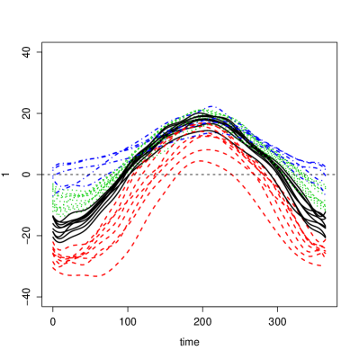
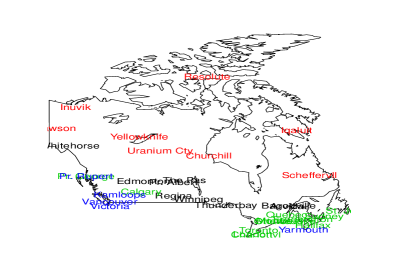
Figure 1: Clustering of the 35 times series of the Canadian temperature data set into 4 groups with pgpEM (left) and geographical positions of the weather stations according to their group belonging (right). The colors indicate the group memberships: group 1 in black, group 2 in red, group 3 in green and group 4 in blue.

It is first interesting to have a look at the name of the weather stations gathered in the different groups formed by pgpEM. It appears that group 1 (black solid curves) is mostly made of continental stations, group 2 (red dashed curves) mostly gathers the stations of the North of Canada, group 3 (green dotted curves) mostly contains the stations of the Atlantic coast whereas the Pacific stations are mostly gathered in group 4 (blue dot-dashed curves). For instance, group 3 contains stations such as Halifax (Nova Scotia) and St Johns (Newfoundland) whereas group 4 has stations such as Vancouver and Victoria (both in British Columbia). The right panel of Figure 1 provides a map of the weather stations where the colors indicate their group membership. This figure shows that the obtained clustering with pgpEM is very satisfying and rather coherent with the actual geographical positions of the stations (the clustering accuracy is 71% here compared with the geographical classification provided by [23]). We recall that the geographical positions of the stations have not been used by pgpEM to provide the partition into 4 groups.

(a) Group 1 (mostly continental stations)

(b) Group 2 (mostly Arctic stations)

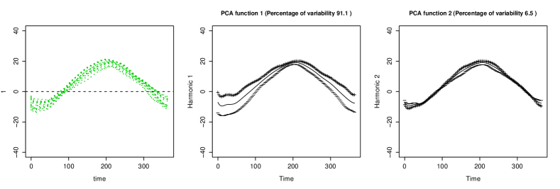
(c) Group 3 (mostly Atlantic stations)

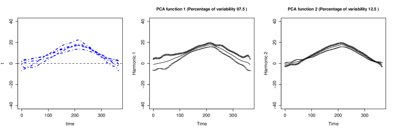
(d) Group 4 (mostly Pacific stations)

Figure 2: The group means of the Canadian temperature data obtained with pgpEM and the effects of adding (+) and subtracting (−) twice the square root of the feature subspace variance (see text for details).

An important characteristic of the groups, but not necessarily easy to visualize, is the specific functional subspace of each group. A classical way to observe principal component functions is to plot the group mean function $\hat{\mu}_{i}(t)$ as well as the functions $\hat{\mu}_{i}(t)\pm 2\sqrt{\hat{\lambda}_{ij}}\hat{q}_{ij}(t)$ (see [23] for more details). Figure 2 shows such a plot for the 4 groups of weather stations formed by pgpEM. It first appears on the first functional principal component of each group that there is more variance between the weather stations in winter than in summer. In particular, the first principal component of group 4 (blue curves, mostly Pacific stations) reveals a specific phenomenon which occurs at the beginning and the end of the winter. Indeed, we can observe a high variance in the temperatures of the Pacific coast stations at these periods of time which can be explained by the presence of mountain stations in this group. The analysis of the second principal components reveals finer phenomena. For instance, the second principal component of group 1 (black curves, mostly continental stations) shows a slight shift between the + and − along the year which indicates a time-shift effect. This may mean that some cities of this group have their seasons shifted, e.g. late entry and exit in the winter. Similarly, the inversion of the + and − on the second principal component of the Pacific and Atlantic groups (blue and green curves) suggests that, for these groups, the coldest cities in winter are also the warmest cities in summer. On the second principal component of group 2 (red curves, mostly Arctic stations), the fact that the + and − curves are almost superimposed shows that the North stations have very similar temperature variations (different temperature means but same amplitude) along the year.

5.3 Classification of networks: the Add Health dataset

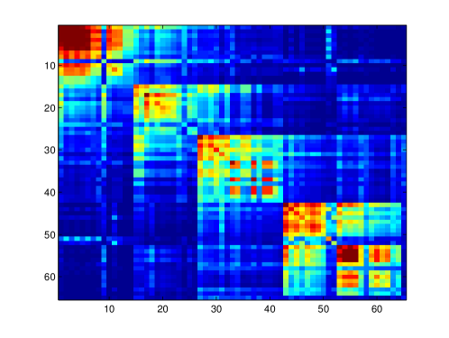
Figure 3: Regularized Laplacian kernel associated to the Add Health network for $\nu=4$: blue pixels correspond to low values (low similarity between nodes) and red pixels correspond to high values (high similarity between nodes).

We now consider network data which are nowadays widely used to represent relationships between persons in organizations or communities. Recently, the need of classifying and visualizing such data has suddenly grown due to the emergence of Internet and of a large number of social network websites. Indeed, increasingly, it is becoming possible to observe “network informations” in a variety of contexts, such as email transactions, connectivity of web pages, protein-protein interactions and social networking. A number of scientific goals can apply to such networks, ranging from unsupervised problems such as describing network structure, to supervised problems such as predicting node labels with information on their relationships.

We investigate here the use of pgpDA to classify the nodes of a network. To our knowledge, only a few kernels (see [29] for more details) have been proposed for network data and the regularized Laplacian kernel is probably the most used. This kernel is defined as follows: let $X$ be a symmetric $n\times n$ socio-matrix where $X_{ij}=1$ if a relationship is observed between the nodes $i$ and $j$ and $X_{ij}=0$ in the opposite case. Let $D$ be the diagonal matrix where $D_{ii}$ indicates the number of relationships for the node $i$, i.e., $D_{ii}=\sum_{j=1}^{n}X_{ij}$. The regularized Laplacian kernel $K$ is then defined by:

$$K=\left[\tilde{L}+\nu I_{n}\right]^{-1},$$

where $\tilde{L}=I_{n}-D^{-\frac{1}{2}}XD^{-\frac{1}{2}}$ is the normalized Laplacian of the network, $\nu$ is a positive value and $I_{n}$ is the identity matrix of size $n$.

The social network studied here is from the National Longitudinal Study of Adolescent Health and it is a part of a big dataset, usually called the “Add Health” dataset. The data were collected in 1994-95 within 80 high-schools and 52 middle schools in the USA. The whole study is detailed in [12]. In addition to personal and social information, each student was asked to nominate his best friends. We consider here the social network based on the answers of 67 students from a single school, treating the grade of each student as the class variable. Two adolescents who nominated nobody were removed from the network. We therefore consider a whole dataset made of 65 students distributed into 5 classes: grade 7 to grade 11.

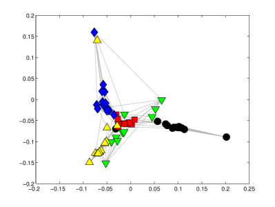
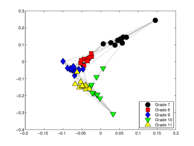
(a) Subspace of class 2	(b) Subspace of class 4

Figure 4: Visualisation of the Add Health network with pgpDA in the feature subspace of the 2nd and the $4$th class (grade 8 and 10 respectively).

We first selected by cross-validation the kernel parameter on a learning sample and the threshold parameter for the intrinsic dimensions was set to $0.2$. The most adapted value for $\nu$ was 4 and this gives on average 96.92% of correct classification for the test nodes. Remark that $\nu$ turned out not to be a sensitive parameter and we obtain satisfying results for a large range of values of $\nu$. Figure 3 presents the kernel associated with the selected value of $\nu$. Since network visualization is an important issue in network analysis, we then kept these parameters to visualize the whole network in the feature subspace of each class. Figure 4 presents the visualization of the network into the feature subspace of the classes 2 and 4. Both visualizations turn out to be very informative and, in particular, the visualization on the feature subspace of the 4th class (grade 10) is particularly useful to understand the network. It is interesting to notice that the network is almost organized along a 1-dimensional manifold (an half-circle here) which is consistent with the nature of the network: students of different classes. The specific form of the representation is due here to some relations between students of grade 7 and 10 (students of the same family perhaps). We also remark that the classes are quite well separated and most of the relationships between students of different classes are between consecutive grades. This suggests that relationships between classes are due to students who failed to move to the upper grade and who may keep contact with old friends. It is in addition interesting to notice that this visualization is very close to the one obtained on the same network by Hoff, Handcock and Raftery in [11] using the so-called “latent space model”.

5.4 Classification of categoretical data: the house-vote dataset

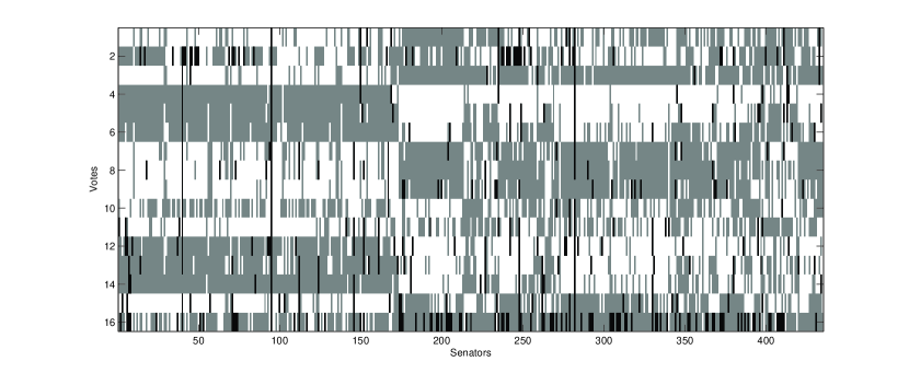
Figure 5: Votes (yea, nay or unknown) for each of the U.S. House of Representatives congressmen on 16 key votes in 1984. Yeas are in indicated in white, nays in gray and missing values in black. The first 168 congressmen are republicans whereas the 267 last ones are democrats.

We focus now on categorical data which are also very frequent in scientific fields. We consider here the task of clustering (unsupervised classification) and therefore the pgpEM algorithm. To evaluate the ability of pgpEM to classify categorical data, we used the U.S. House Votes data set from the UCI repository. This data set is a record of the votes (yea, nay or unknown) for each of the U.S. House of Representatives congressmen on 16 key votes in 1984. These data were recorded during the during the third and fourth years of Ronald Reagan’s Presidency. At this time, the republicans controlled the Senate, while the democrats controlled the House of Representatives. Figure 5 shows the database where yeas are in indicated in white, nays in gray and missing values in black. The first 168 congressmen are republicans whereas the 267 last ones are democrats. As we can see, the considered votes are very discriminative since republicans and democrats vote differently in almost all cases while most of the congressmen follow the majority vote in their group. We can however notice that a significant part (around 50 congressmen) of the democrats tend to vote differently from the other democrats.

To cluster this dataset, we first build a kernel from the categorical observations (16 qualitative variables with 3 possible values: yea, nay or ?). We chose a kernel, proposed in [7], based on the Hamming distance which measures the minimum number of substitutions required to change one observation into another one. Figure 6 presents the resulting kernel (left panel) and the clustering result obtained with the pgpEM algorithm. The clustering results are presented through a binary matrix where a black pixel indicates a common membership between two senators and a white pixel means different memberships for the two senators. The pgpEM algorithm was used with the model $\mathcal{M}_{0}$, with a number of group equals to 2 and the Cattell’s threshold was set to 0.2. The clustering accuracy between the obtained partition of the data and the democrat/republican partition was 84.37% on this example. As one can observe, the pgpEM algorithm globally succeeds in recovering the partition of the House of Representatives. It is also interesting to notice that most of the congressmen which are not correctly classified are those who tend to vote differently from the majority vote in their group. Finally, the pgpEM algorithm allows to visualize the observed categorical data into the (quantitative) feature subspace of the two groups. Figure 7 presents these visualizations. The observation of these two plots confirms the fact that republicans voted more homogeneously than democrats in 1984 since there is no clear concentration of points on both plots for the democrats.

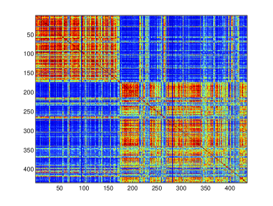
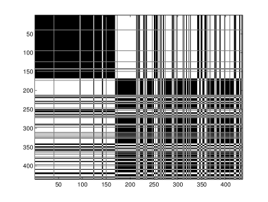
Figure 6: Kernel based on the Hamming distance (left) computed on the house-vote dataset and clustering results (right) obtained with pgpEM. For the kernel, blue and red pixels correspond respectively to low and high values. The clustering results are presented through a binary matrix where a black pixel indicates a common membership between two senators.

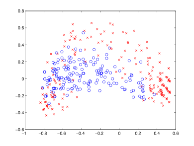
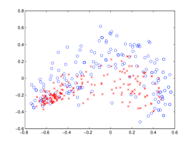
Figure 7: Visualization of the house-vote data in the feature subspace of the republican (left) and the democrat (right) groups (red crosses denote republicans and blue circles denote democrats).

5.5 Classification of mixed data: the Thyroid dataset

In this final experiment, we consider the supervised classification of mixed data which is more and more a frequent case. Indeed, it is usual to collect for the same individuals both quantitative and categorical data. For instance, in Medicine, several quantitative features can be measured for a patient (blood test results, blood pressure, morphological characteristics, …) and these data can be completed by answers of the patient on its general health conditions (pregnancy, surgery, tabacco, …). The Thyroid dataset considered here is from the UCI repository and contains thyroid disease records supplied by the Garavan Institute, Sydney, Australia. The dataset contains 665 records on male patients for which the answers (true of false) on 14 questions have been collected as well as 6 blood test results (quantitative measures). Among the 665 patients of the study, 61 suffer from a thyroid disease.

To make pgpDA able to deal with such data, we built a combined kernel by mixing a kernel based on the Hamming distance [7] (same kernel as in the previous section) for the categorical features and a Gaussian kernel for the quantitative data. We chose to combine both kernels simply as follows:

$$K(x_{j},x_{\ell})=\alpha K_{1}(x_{j},x_{\ell})+(1-\alpha)K_{2}(x_{j},x_{\ell}),$$

where $K_{1}$ and $K_{2}$ are the kernels computed respectively on the categorical and quantitative features. Another solution would be to multiply both kernels. We refer to [18] for further details on multiple kernel learning.

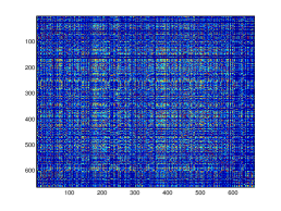
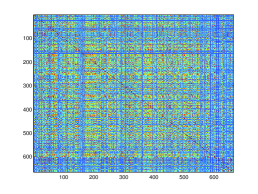
Quantitative data kernel	Categorical data kernel	Combined kernel

Figure 8: Quantitative (left) and categorical (center) data kernels and the combined kernel (right) for the Thyroid dataset (mixed data).

We selected the optimal set of kernel parameters by cross-validation on a learning part of the data. The model for pgpDA was the model $\mathcal{M}_{0}$ with the Cattell’s threshold set to $0.2$. The mixing parameter $\alpha$ for kernels was set to $0.5$ in order not to favor any kernel but it is expected an improvement of the results if this parameter is tuned too. Kernel parameters have been tuned by cross-validation on a learning sample and the kernels associated to these values are presented in Figure 8. The rows and columns of the matrices are sorted according to the class memberships (healthy or sick) and the sick patients are the last ones. We then compared the performance of pgpDA with the combined kernel to pgpDA with, on the one hand, a simple RBF kernel built only on the quantitative variables of the dataset and, on the other hand, a Hamming kernel built only on the categorical variables. Table 4 presents both the true positive (TP) and false positive (FP) rates obtained on 25 replications of the classification experiment for pgpDA on quantitative data, on categorical data and on the mixed data. It turns out that quantitative data contains most of the important information to discriminate the patients with thyroid diseases and that categorical data, when considered alone, are not enough to build an efficient classifier. However, it appears that the use of the categorical features in combination with the quantitative data allows to slightly improve the prediction of thyroid diseases (increases the TP rate and decreases the FP rate). In particular, the reduction of the FP rate is important here since it implies an important reduction of the number of false alarms.

Method	pgpDA on quantitative data	pgpDA on categorical data	pgpDA with the combined kernel
TP rate	74.86	96.00	75.88
FP rate	22.16	95.53	21.97

Table 4: Classification results on test sets for the Thyroid dataset (mixed data). Results are averaged on 25 replications of the experiment.

6 Conclusion

This work has introduced a family of parsimonious Gaussian process models for the supervised and unsupervised classification of quantitative and non-quantitative data. The proposed parsimonious models are obtained by constraining the eigen-decomposition of the Gaussian processes modeling each class. They allow in particular to use non-linear mapping functions which project the observations into an infinite dimensional space and to build, from a finite sample, a model-based classifier in this space. It has been also demonstrated that the building of the classifier can be directly done from the observation space through a kernel, avoiding the explicit knowledge of the mapping function. It has been possible to classify data of various nature including categorical data, functional data, networks and even mixed data by combining different kernels. The methodology is as well extended to the unsupervised classification case. Numerical experiments on benchmark data sets have shown that pgpDA performs similarly or better compared to the best kernel methods of the state of the art. The possibility to examine the model parameters and to visualize the data into the class-specific feature subspaces permits a finer interpretation of the results than with conventional discriminative kernel methods. Among the possible extensions of this work, it would be interesting to extend the methodology to the semi-supervised case in which only a few observations are labeled.

Appendix: Proofs

Proof of Proposition 1

Recalling that $d_{\max}=\max(d_{1},...,d_{k})$, the classification function can be rewritten as:

$$D_{i}(\varphi(x))=\sum_{j=1}^{r}\frac{1}{\lambda_{ij}}<\varphi(x)-\mu_{i},q_{ij}>_{L_{2}}^{2}+\sum_{j=1}^{d_{i}}\log(\lambda_{ij})+\sum_{j=d_{i}+1}^{d_{\max}}\log(\lambda)-2\log(\pi_{i})+\gamma,$$

where $\gamma=(r-d_{\max})\log(\lambda)$ is a constant term which does not depend on the index $i$ of the class. In view of the assumptions, $D_{i}(\varphi(x))$ can be also rewritten as:

$$D_{i}(\varphi(x)) = \sum_{j=1}^{d_{i}}\frac{1}{\lambda_{ij}}<\varphi(x)-\mu_{i},q_{ij}>_{L_{2}}^{2}+\frac{1}{\lambda}\sum_{j=d_{i}+1}^{r}<\varphi(x)-\mu_{i},q_{ij}>_{L_{2}}^{2}$$

$$+ \sum_{j=1}^{d_{i}}\log(\lambda_{ij})+(d_{\max}-d_{i})\log(\lambda)-2\log(\pi_{i})+\gamma.$$

Introducing the norm $||.||_{L_{2}}$ associated with the scalar product $<.,.>_{L_{2}}$ and in view of Proposition 1 of [28, p. 208], we finally obtain:

$$D_{i}(\varphi(x)) = \sum_{j=1}^{d_{i}}\left(\frac{1}{\lambda_{ij}}-\frac{1}{\lambda}\right)<\varphi(x)-\mu_{i},q_{ij}>_{L_{2}}^{2}+\frac{1}{\lambda}||\varphi(x)-\mu_{i}||_{L_{2}}^{2}$$

$$+ \sum_{j=1}^{d_{i}}\log(\lambda_{ij})+(d_{\max}-d_{i})\log(\lambda)-2\log(\pi_{i})+\gamma,$$

which is the desired result. $\square$

Proof of Proposition 2

The proof involves three steps.

i) Computation of the projection $<\varphi(x)-\hat{\mu}_{i},\hat{q}_{ij}>_{L_{2}}$ : Since $(\hat{\lambda}_{ij},\hat{q}_{ij})$ is solution of the Fredholm-type equation, it follows that, for all $t\in[0,1]$,

$$\hat{\lambda}_{ij}\hat{q}_{ij}(t) = \int_{0}^{1}\hat{\Sigma}_{i}(s,t)\hat{q}_{ij}(s)ds$$ (9)

$$= \frac{1}{n_{i}}\sum_{x_{\ell}\in C_{i}}<\varphi(x_{\ell})-\hat{\mu}_{i},\hat{q}_{ij}>_{L_{2}}(\varphi(x_{\ell})(t)-\hat{\mu}_{i}(t)).$$

This implies that $\hat{q}_{ij}$ lies in the linear subspace spanned by the $(\varphi(x_{\ell})-\hat{\mu}_{i})$, $x_{\ell}\in C_{i}$. As a consequence, the rank of the operator $\hat{\Sigma}_{i}$ is finite and is at most $r_{i}=\min(n_{i},r)$. It therefore exists $\beta_{ij\ell}\in{\mathbb{R}}$ such that:

$$\hat{q}_{ij}=\frac{1}{\sqrt{n_{i}\hat{\lambda}_{ij}}}\sum_{x_{\ell}\in C_{i}}\beta_{ij\ell}(\varphi(x_{\ell})-\hat{\mu}_{i})$$ (10)

leading to:

$$<\varphi(x)-\hat{\mu}_{i},\hat{q}_{ij}>_{L_{2}}=\frac{1}{\sqrt{n_{i}\hat{\lambda}_{ij}}}\sum_{x_{\ell}\in C_{i}}\beta_{ij\ell}\rho_{i}(x,x_{\ell}),$$ (11)

for all $j=1,\dots,r_{i}$. The estimated classification function has therefore the following form:

$$\hat{D}_{i}(\varphi(x)) =\frac{1}{n_{i}}\sum_{j=1}^{d_{i}}\frac{1}{\hat{\lambda}_{ij}}\left(\frac{1}{\hat{\lambda}_{ij}}-\frac{1}{\hat{\lambda}}\right)\left(\sum_{x_{\ell}\in C_{i}}\beta_{ij\ell}\rho_{i}(x,x_{\ell})\right)^{2}+\frac{1}{\hat{\lambda}}\rho_{i}(x,x)$$

$$+\sum_{j=1}^{d_{i}}\log(\hat{\lambda}_{ij})+(d_{\max}-d_{i})\log(\hat{\lambda})-2\log(\hat{\pi}_{i}),$$

for all $i=1,\dots,k$.

ii) Computation of the $\beta_{ij\ell}$ and $\hat{\lambda}_{ij}$: Replacing (10) in the Fredholm-type equation (9) it follows that

$$\frac{1}{n_{i}}\sum_{x_{\ell},x_{\ell^{\prime}}\in C_{i}}\beta_{ij\ell^{\prime}}(\varphi(x_{\ell})-\hat{\mu}_{i})\rho_{i}(x_{\ell},x_{\ell^{\prime}})=\hat{\lambda}_{ij}\sum_{x_{\ell^{\prime}}\in C_{i}}\beta_{ij\ell^{\prime}}(\varphi(x_{\ell^{\prime}})-\hat{\mu}_{i}).$$

Finally, projecting this equation on $\varphi(x_{m})-\hat{\mu}_{i}$ for $x_{m}\in C_{i}$ yields

$$\frac{1}{n_{i}}\sum_{x_{\ell},x_{\ell^{\prime}}\in C_{i}}\beta_{ij\ell^{\prime}}\rho_{i}(x_{\ell},x_{m})\rho_{i}(x_{\ell},x_{\ell^{\prime}})=\hat{\lambda}_{ij}\sum_{x_{\ell^{\prime}}\in C_{i}}\beta_{ij\ell^{\prime}}\rho_{i}(x_{m},x_{\ell^{\prime}}).$$

Recalling that $M_{i}$ is the matrix $n_{i}\times n_{i}$ defined by $(M_{i})_{\ell,\ell^{\prime}}=\rho_{i}(x_{\ell},x_{\ell^{\prime}})/n_{i}$ and introducing $\beta_{ij}$ the vector of ${\mathbb{R}}^{n_{i}}$ defined by $(\beta_{ij})_{\ell}=\beta_{ij\ell}$, the above equation can be rewritten as $M_{i}^{2}\beta_{ij}=\hat{\lambda}_{ij}M_{i}\beta_{ij}$ or, after simplification $M_{i}\beta_{ij}=\hat{\lambda}_{ij}\beta_{ij}.$ As a consequence, $\hat{\lambda}_{ij}$ is the $j$th largest eigenvalue of $M_{i}$ and $\beta_{ij}$ is the associated eigenvector for all $1\leq j\leq d_{i}$. Let us note that the constraint $\|\hat{q}_{ij}\|=1$ can be rewritten as $\beta_{ij}^{t}\beta_{ij}=1$.

iii) Computation of $\hat{\lambda}$: Remarking that trace$(\hat{\Sigma}_{i})=\mbox{trace$(M_{i})+\mbox{$\sum_{j=r_{i}+1}^{r}\hat{\lambda}_{ij}$}$}$, it follows:

$$\hat{\lambda}=\frac{1}{\sum_{i=1}^{k}\hat{\pi_{i}}(r_{i}-d_{i})}\sum_{i=1}^{k}\hat{\pi}_{i}\left(\mathrm{trace}(M_{i})-\sum_{j=1}^{d_{i}}\hat{\lambda}_{ij}\right),$$

and the proposition is proved. $\square$

Proof of Proposition 3

It is sufficient to prove that $\hat{q}_{ij}$ and $\hat{\lambda}_{ij}$ are respectively the $j$th normed eigenvector and eigenvalue of $\hat{\Sigma}_{i}$. First,

$$\hat{\Sigma}_{i}\hat{q}_{ij} =\frac{1}{\sqrt{n_{i}\hat{\lambda}_{ij}}}\frac{1}{n_{i}}\sum_{x_{\ell^{\prime}}\in C_{i}}(x_{\ell^{\prime}}-\bar{\mu}_{i})(x_{\ell^{\prime}}-\bar{\mu}_{i})^{t}\sum_{x_{\ell}\in C_{i}}\beta_{ij\ell}(x_{\ell}-\bar{\mu}_{i})$$

$$=\frac{1}{\sqrt{n_{i}\hat{\lambda}_{ij}}}\frac{1}{n_{i}}\sum_{x_{\ell^{\prime}},x_{\ell}\in C_{i}}\beta_{ij\ell}(x_{\ell^{\prime}}-\bar{\mu}_{i})(x_{\ell^{\prime}}-\bar{\mu}_{i})^{t}(x_{\ell}-\bar{\mu}_{i})$$

$$=\frac{1}{\sqrt{n_{i}\hat{\lambda}_{ij}}}\frac{1}{n_{i}}\sum_{x_{\ell^{\prime}},x_{\ell}\in C_{i}}\beta_{ij\ell}(x_{\ell^{\prime}}-\bar{\mu}_{i})\rho_{i}(x_{\ell},x_{\ell^{\prime}})$$

$$=\frac{1}{\sqrt{n_{i}\hat{\lambda}_{ij}}}\sum_{x_{\ell^{\prime}},x_{\ell}\in C_{i}}(M_{i})_{\ell,\ell^{\prime}}\beta_{ij\ell}(x_{\ell^{\prime}}-\bar{\mu}_{i})$$

$$=\frac{1}{\sqrt{n_{i}\hat{\lambda}_{ij}}}B^{-1}\sum_{x_{\ell^{\prime}}\in C_{i}}(M_{i}\beta_{ij})_{\ell^{\prime}}(x_{\ell^{\prime}}-\bar{\mu}_{i}),$$

and remarking that $\beta_{ij}$ is eigenvector of $M_{i}$, it follows:

$$\hat{\Sigma}_{i}\hat{q}_{ij}=\hat{\lambda}_{ij}\frac{1}{\sqrt{n_{i}\hat{\lambda}_{ij}}}B^{-1}\sum_{x_{\ell^{\prime}}\in C_{i}}\beta_{ij\ell^{\prime}}(x_{\ell^{\prime}}-\bar{\mu}_{i})=\hat{\lambda}_{ij}\hat{q}_{ij}.$$

Second, straightforward algebra shows that

$$||\hat{q}_{ij}||^{2} =\frac{1}{n_{i}\hat{\lambda}_{ij}}\sum_{x_{\ell}\in C_{i}}\beta_{ij\ell}(x_{\ell})-\bar{\mu}_{i})^{t}\sum_{x_{\ell^{\prime}}\in C_{i}}\beta_{ij\ell^{\prime}}(x_{\ell^{\prime}}-\bar{\mu}_{i})$$

$$=\frac{1}{n_{i}\hat{\lambda}_{ij}}\sum_{x_{\ell^{\prime}},x_{\ell}\in C_{i}}\beta_{ij\ell}\beta_{ij\ell^{\prime}}(x_{\ell}-\bar{\mu}_{i})^{t}(x_{\ell^{\prime}}-\bar{\mu}_{i})$$

$$=\frac{1}{\hat{\lambda}_{ij}}\sum_{x_{\ell^{\prime}},x_{\ell}\in C_{i}}(M_{i})_{\ell,\ell^{\prime}}\beta_{ij\ell}\beta_{ij\ell^{\prime}}$$

$$=\frac{1}{\hat{\lambda}_{ij}}\hat{q}_{ij}^{t}M_{i}\hat{q}_{ij}=1,$$

and the result is proved. $\square$

Proof of Proposition 4

For all $\ell=1,\dots,L$, the $\ell$th coordinate of the mapping function $\varphi(x)$ is defined as the $\ell$th coordinate of the function $x$ expressed in the truncated basis $\{b_{1},\dots,b_{L}\}$. More specifically,

$$x(t)=\sum_{\ell=1}^{L}\varphi_{\ell}(x)b_{\ell}(t),$$

for all $t\in[0,1]$ and thus, for all $j=1,\dots,L$, we have

$$\gamma_{j}(x)=\int_{0}^{1}x(t)b_{j}(t)dt=\sum_{\ell=1}^{L}\varphi_{\ell}(x)\int_{0}^{1}b_{j}(t)b_{\ell}(t)dt=\sum_{\ell=1}^{L}B_{j\ell}\varphi_{\ell}(x).$$

As a consequence, $\varphi(x)=B^{-1}\gamma(x)$ and $K(x,y)=\gamma(x)^{t}B^{-1}\gamma(y)$. Introducing

$$\bar{\gamma}_{i}=\frac{1}{n_{i}}\sum_{x_{j}\in C_{i}}\gamma(x_{j}),$$

it follows that $\rho_{i}(x,y)=(\gamma(x)-\bar{\gamma}_{i})^{t}B^{-1}(\gamma(y)-\bar{\gamma}_{i})$. Let us first show that $\hat{q}_{ij}$ is eigenvector of $B^{-1}\hat{\Sigma}_{i}$. Recalling that

$$\hat{q}_{ij}=\frac{1}{\sqrt{n_{i}\hat{\lambda}_{ij}}}B^{-1}\sum_{x_{\ell}\in C_{i}}\beta_{ij\ell}(\gamma(x_{\ell})-\bar{\gamma}_{i}),$$

we have

$$B^{-1}\hat{\Sigma}_{i}\hat{q}_{ij} =\frac{1}{\sqrt{n_{i}\hat{\lambda}_{ij}}}B^{-1}\frac{1}{n_{i}}\sum_{x_{\ell^{\prime}}\in C_{i}}(\gamma(x_{\ell^{\prime}})-\bar{\gamma}_{i})(\gamma(x_{\ell^{\prime}})-\bar{\gamma}_{i})^{t}B^{-1}\sum_{x_{\ell}\in C_{i}}\beta_{ij\ell}(\gamma(x_{\ell})-\bar{\gamma}_{i})$$

$$=\frac{1}{\sqrt{n_{i}\hat{\lambda}_{ij}}}B^{-1}\frac{1}{n_{i}}\sum_{x_{\ell^{\prime}},x_{\ell}\in C_{i}}\beta_{ij\ell}(\gamma(x_{\ell^{\prime}})-\bar{\gamma}_{i})(\gamma(x_{\ell^{\prime}})-\bar{\gamma}_{i})^{t}B^{-1}(\gamma(x_{\ell})-\bar{\gamma}_{i})$$

$$=\frac{1}{\sqrt{n_{i}\hat{\lambda}_{ij}}}B^{-1}\frac{1}{n_{i}}\sum_{x_{\ell^{\prime}},x_{\ell}\in C_{i}}\beta_{ij\ell}(\gamma(x_{\ell^{\prime}})-\bar{\gamma}_{i})\rho_{i}(x_{\ell},x_{\ell^{\prime}})$$

$$=\frac{1}{\sqrt{n_{i}\hat{\lambda}_{ij}}}B^{-1}\sum_{x_{\ell^{\prime}},x_{\ell}\in C_{i}}(M_{i})_{\ell,\ell^{\prime}}\beta_{ij\ell}(\gamma(x_{\ell^{\prime}})-\bar{\gamma}_{i})$$

$$=\frac{1}{\sqrt{n_{i}\hat{\lambda}_{ij}}}B^{-1}\sum_{x_{\ell^{\prime}}\in C_{i}}(M_{i}\beta_{ij})_{\ell^{\prime}}(\gamma(x_{\ell^{\prime}})-\bar{\gamma}_{i}).$$

Remarking that $\beta_{ij}$ is eigenvector of $M_{i}$, it follows:

$$B^{-1}\hat{\Sigma}_{i}\hat{q}_{ij}=\hat{\lambda}_{ij}\frac{1}{\sqrt{n_{i}\hat{\lambda}_{ij}}}B^{-1}\sum_{x_{\ell^{\prime}}\in C_{i}}\beta_{ij\ell^{\prime}}(\gamma(x_{\ell^{\prime}})-\bar{\gamma}_{i})=\hat{\lambda}_{ij}\hat{q}_{ij}.$$

Let us finally compute the norm of $\hat{q}_{ij}$:

$$||\hat{q}_{ij}||^{2} =\frac{1}{n_{i}\hat{\lambda}_{ij}}\sum_{x_{\ell}\in C_{i}}\beta_{ij\ell}(\gamma(x_{\ell})-\bar{\gamma}_{i})^{t}B^{-1}\sum_{x_{\ell^{\prime}}\in C_{i}}\beta_{ij\ell^{\prime}}(\gamma(x_{\ell^{\prime}})-\bar{\gamma}_{i})$$

$$=\frac{1}{n_{i}\hat{\lambda}_{ij}}\sum_{x_{\ell^{\prime}},x_{\ell}\in C_{i}}\beta_{ij\ell}\beta_{ij\ell^{\prime}}(\gamma(x_{\ell})-\bar{\gamma}_{i})^{t}B^{-1}(\gamma(x_{\ell^{\prime}})-\bar{\gamma}_{i})$$

$$=\frac{1}{\hat{\lambda}_{ij}}\sum_{x_{\ell^{\prime}},x_{\ell}\in C_{i}}(M_{i})_{\ell,\ell^{\prime}}\beta_{ij\ell}\beta_{ij\ell^{\prime}}$$

$$=\frac{1}{\hat{\lambda}_{ij}}\hat{q}_{ij}^{t}M_{i}\hat{q}_{ij}=1,$$

and the result is proved. $\square$

References

- [1] C. Bouveyron and C. Brunet. Simultaneous model-based clustering and visualization in the Fisher discriminative subspace. Statistics and Computing, 22(1):301–324, 2012.
- [2] C. Bouveyron, S. Girard, and C. Schmid. High Dimensional Data Clustering. Computational Statistics and Data Analysis, 52:502–519, 2007.
- [3] C. Bouveyron, S. Girard, and C. Schmid. High-Dimensional Discriminant Analysis. Communication in Statistics: Theory and Methods, 36:2607–2623, 2007.
- [4] C. Bouveyron and J. Jacques. Model-based clustering of time series in group-specific functional subspaces. Advances in Data Analysis and Classification, 5(4):281–300, 2011.
- [5] R. Cattell. The scree test for the number of factors. Multivariate Behavioral Research, 1(2):245–276, 1966.
- [6] O. Chapelle, B. Schölkopf, and A. Zien, editors. Semi-Supervised Learning. MIT Press, Cambridge, MA, 2006.
- [7] J. Couto. Kernel k-means for categorical data. In Advances in Intelligent Data Analysis VI, volume 3646 of Lecture Notes in Computer Science, pages 739–739. 2005.
- [8] A. Dempster, N. Laird, and D. Rubin. Maximum likelihood from incomplete data via the EM algorithm. Journal of the Royal Statistical Society, Series B, 39(1):1–38, 1977.
- [9] M.M. Dundar and D.A. Landgrebe. Toward an optimal supervised classifier for the analysis of hyperspectral data. IEEE Transactions on Geoscience and Remote Sensing, 42(1):271 – 277, jan. 2004.
- [10] R.A. Fisher. The use of multiple measurements in taxonomic problems. Annals of Eugenics, 7:179–188, 1936.
- [11] M. Handcock, A. Raftery, and J. Tantrum. Model-based clustering for social networks. Journal of the Royal Statistical Society, Series A, 170(2):1–22, 2007.
- [12] Harris, K. et al. The national longitudinal of adolescent health: research design. Technical report, Carolina Population Center, University of North Carolina, 2003.
- [13] T. Hofmann, B. Schölkopf, and A. Smola. Kernel methods in machine learning. Annals of Statistics, 36(3):1171–1220, 2008.
- [14] I. Kwang, M. Franz, and B. Scholkopf. Iterative kernel principal component analysis for image modeling. IEEE Transactions on Pattern Analysis and Machine Intelligence, 27(9):1351 –1366, 2005.
- [15] G. McLachlan. Discriminant Analysis and Statistical Pattern Recognition. Wiley, New York, 1992.
- [16] G. McLachlan, D. Peel, and R. Bean. Modelling high-dimensional data by mixtures of factor analyzers. Computational Statistics and Data Analysis, 41:379–388, 2003.
- [17] P. McNicholas and B. Murphy. Parsimonious Gaussian mixture models. Statistics and Computing, 18(3):285–296, 2008.
- [18] G Mehmet and E. Alpaydin. Multiple kernel learning algorithms. Journal of Machine Learning Research, 12:2211–2268, 2011.
- [19] S. Mika, G. Ratsch, J. Weston, B. Schölkopf, and K.R. Müllers. Fisher discriminant analysis with kernels. In Neural Networks for Signal Processing, pages 41–48, 1999.
- [20] A. Montanari and C. Viroli. Heteroscedastic Factor Mixture Analysis. Statistical Modeling: An International journal, 10(4):441–460, 2010.
- [21] T.B. Murphy, N. Dean, and A.E. Raftery. Variable Selection and Updating in Model-Based Discriminant Analysis for High Dimensional Data with Food Authenticity Applications. Annals of Applied Statistics, 4(1):219–223, 2010.
- [22] E. Pekalska and B. Haasdonk. Kernel discriminant analysis for positive definite and indefinite kernels. IEEE Transactions on Pattern Analysis and Machine Intelligence, 31(6):1017 –1032, 2009.
- [23] J. O. Ramsay and B. W. Silverman. Functional data analysis. Springer Series in Statistics. Springer, New York, second edition, 2005.
- [24] B. Scholkopf and A. Smola. Learning with Kernels: Support Vector Machines, Regularization, Optimization, and Beyond. MIT Press, Cambridge, MA, USA, 2001.
- [25] B. Schölkopf, A. Smola, and K-R. Müller. Nonlinear component analysis as a kernel eigenvalue problem. Neural Computation, 10(5):1299–1319, 1998.
- [26] B. Schölkopf, K. Tsuda, and J.-P. Vert, editors. Kernel Methods in Computational Biology. MIT Press, Cambridge, MA, 2004.
- [27] J. Shawe-Taylor and N. Cristianini. Kernel Methods for Pattern Analysis. Cambridge University Press, 2004.
- [28] G.R. Shorack and J.A. Wellner. Empirical Processes with Applications to Statistics. Wiley, New York, 1986.
- [29] A. Smola and R. Kondor. Kernels and regularization on graphs. In Proc. Conf. on Learning Theory and Kernel Machines, pages 144–158, 2003.