Ordering of the Heisenberg spin glass in four dimensions
Abstract
Ordering of the Heisenberg spin glass in four dimensions (4D) with the nearest-neighbor Gaussian coupling is investigated by equilibrium Monte Carlo simulations, with particular attention to its spin and chiral orderings. It is found that the spin and the chirality order simultaneously with a common correlation-length exponent , i.e., the absence of the spin-chirality decoupling in 4D. Yet, the spin-glass ordered state exhibits a nontrivial phase-space structure associated with a continuous one-step-like replica-symmetry breaking, different in nature from that of the Ising spin glass or of the mean-field spin glass. Comparison is made with the ordering of the Heisenberg spin glass in 3D, and with that of the 1D Heisenberg spin glass with a long-range power-law interaction. It is argued that the 4D might be close to the marginal dimension separating the spin-chirality decoupling/coupling regimes.
I I. Introduction
The Heisenberg spin-glass (SG) model, or the Edwards-Anderson model with the isotropic Heisenberg exchange interaction EA , has been considered as the standard model of many real SG materials review . In realistic three spatial dimensions (3D), earlier studies in the 80’s suggested that the isotropic Heisenberg SG did not exhibit an equilibrium SG transition at any finite temperature in apparent contrast to experiments Banavar82 ; McMillan85 ; Olive86 ; Matsubara91 ; Yoshino93 . Then, a proposal was made in 1992 that the model might exhibit a finite-temperature transition in the chiral sector, with the standard SG order occurring at a temperature lower than the chiral-glass (CG) ordering temperature , i.e., Kawamura92 . The occurrence of such separate spin and chirality transitions is now called “spin-chirality decoupling” Kawamura10 . Chirality is a multispin variable representing the sense or the handedness of local noncoplanar spin structures induced by spin frustration. A possible counter-view to such a picture might be that the spin and the chirality order at a common finite temperature Matsubara ; LeeYoung03 ; Campos06 ; LeeYoung07 ; Fernandez09 . Although there is no complete consensus, recent simulations point to the occurrence of the spin-chirality decoupling in 3D Matsumoto02 ; HukuKawa05 ; Campbell07 ; VietKawamura09a ; VietKawamura09b . For example, Ref.VietKawamura09b reported that was lower than by about %.
To get further insight into the issue, it might be useful to extend the space dimension from original to general -dimensions. In , the Heisenberg SG with a short-range (SR) interaction exhibits only a transition. In , recent calculations suggested that the vector SG model, either the three-component Heisenberg SG KawaYone03 or the two-component XY SG Weigel08 , exhibited a transition but with the spin-chirality decoupling, i.e., the CG correlation-length exponent was greater than the SG correlation-length exponent , meaning that this transition was characterized by two distinct diverging length scales, each associated with the chirality and with the spin. In the opposite limit of , the model is known to reduce to the mean-field (MF) model, i.e., the Sherrington-Kirkpatrick (SK) model. The Heisenberg SK model is known to exhibit a single finite-temperature transition, with no spin-chirality decoupling. In high but finite , Monte Carlo (MC) study by Imagawa and Kawamura suggested that the spin-chirality decoupling did not occur for , whereas the situation in appeared somewhat more marginal ImaKawa03a .
Another useful way of attacking the issue might be to study the one-dimensional (1D) Heisenberg SG with a long-range (LR) power-law interaction proportional to ( the spin distance). Indeed, several studies both for the Ising and the Heisenberg SGs suggested that the 1D LR SG model with a power-law exponent might show the ordering behavior analogous to the -dimensional SG model with a SR interaction BinderYoung86 ; Katzgraber03 ; Katzgraber05 ; Katzgraber09 ; Leuzzi99 ; Leuzzi08 ; VietKawamura10a ; VietKawamura10b ; SharmaYoung . Even a simple empirical formula relating and , , was proposed BinderYoung86 , though the relation is only approximate.
Recent MC calculation on the 1D LR Heisenberg SG by Viet and Kawamura suggested that the spin-chirality decoupling occurred for , but did not occur for , being estimated numerically to be VietKawamura10a ; VietKawamura10b . If one applies the approximate correspondence formula quoted above BinderYoung86 , the critical dimension below which the spin-chirality decoupling is expected would be , suggesting that might lie near the margin of, slightly on the side of the spin-chirality coupling regime. Of course, the above correspondence formula is only approximate, and even whether is greater or smaller than is not clear. Previous simulation on the Heisenberg SG, which dealt with the linear size of , was not definitive concerning the occurrence of the spin-chirality decoupling in 4D ImaKawa03a .
Under such circumstances, the purpose of the present paper is first to clarify whether the spin and the chirality are decoupled or not in the Heisenberg SG by simulating larger systems than the ones studied in Ref.ImaKawa03a . Since is expected to be close to the marginal dimension concerning the spin-chirality decoupling, we wish to see what kind of ordering behavior is realized for the spin and the chirality near the marginal dimension.
The present paper is organized as follows. In §II, we introduce our model and explain some of the details of our MC simulation. Various physical quantities are defined in §III. The results of our MC simulations, including the spin and the chiral correlation lengths, the spin and the chiral Binder ratios, are presented in §IV. The SG and CG transition temperatures are determined by carefully examining the size dependence of the finite-size data. In §V, critical properties of the spin and of the chirality are investigated by means of a finite-size scaling analysis. Finally, section §VI is devoted to summary and discussion.
II II. The model and the method
The model we consider is the isotropic classical Heisenberg model on a 4D hyper-cubic lattice, with the nearest-neighbor Gaussian coupling. The Hamiltonian is given by
| (1) |
where is a three-component unit vector, and sum is taken over nearest-neighbor pairs on the lattice. The nearest-neighbor coupling is assumed to obey the Gaussian distribution with zero mean and variance , which is taken to be unity () in the following. The temperature is measured in units of .
We perform equilibrium MC simulations on the model. The lattices are hyper-cubic lattices with sites with , 8, 10, 12, 16 and 20. We impose periodic boundary conditions in all four directions. Sample average is taken over 1300, 1200, 840, 590, 430 and 256 independent bond realizations for , 8, 10, 12, 16 and 20, respectively. Error bars of physical quantities are estimated by sample-to-sample statistical fluctuations over the bond realization.
In order to facilitate efficient thermalization, we combine the heat-bath and the over-relaxation methods with the temperature-exchange technique HukushimaNemoto . For each heat-bath sweep we perform 11, 15, 19, 23, 31 and 55 over-relaxation sweeps, while the total number of temperature points in the temperature-exchange process are taken to be 35, 51, 59, 55, 55 and 60 for , 8, 10, 12, 16 and 20, respectively. Care is taken to be sure that the system is fully equilibrated. Equilibration is checked by following the procedures of Ref.VietKawamura09b .
III III. Physical quantities
In this section, we define various physical quantities measured in our simulations.
For the Heisenberg spin, the local chirality at the -th site and in the -th direction may be defined for three neighboring Heisenberg spins by a scalar
| (2) |
where denotes a unit vector along the -th axis. There are in total local chiral variables.
We define an “overlap” for the chirality. We prepare at each temperature two independent systems 1 and 2 described by the same Hamiltonian (1) with the same interaction set. We simulate these two independent systems 1 and 2 in parallel with using different spin initial conditions and different sequences of random numbers.
The -dependent chiral overlap, , is defined as an overlap variable between the two replicas 1 and 2 as a scalar
| (3) |
where the upper suffixes (1) and (2) denote the two replicas of the system, and is the position vector of the site .
The -dependent spin overlap, , is defined by a tensor variable between the and components of the Heisenberg spin,
| (4) |
In term of the -dependent overlap, the CG and the SG order parameters are defined by the second moment of the overlap at a wavevector ,
| (5) |
| (6) |
where represents a thermal average and an average over the bond disorder. The CG order parameter has been normalized here by the mean-square amplitude of the local chirality,
| (7) |
which remains nonzero only when the spin has a noncoplanar structure locally. The local-chirality amplitude depends on the temperature and the lattice size only weakly.
Finite-size correlation length is defined by
| (8) |
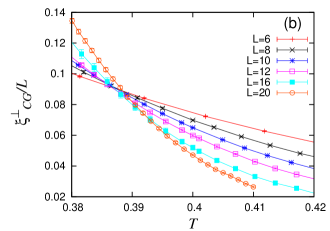
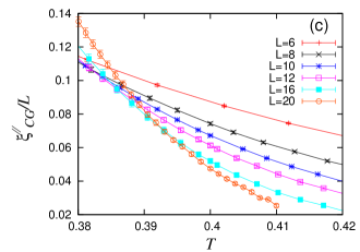
for each case of the chirality and the spin, and , where with . For the CG correlation length , we consider two distinct definitions depending on the mutual direction between the -vector appearing in the definition of the local chirality (2) and the -vector. When , i.e., , we call the corresponding the parallel CG correlation length , whereas, when , i.e., , we call the corresponding the perpendicular CG correlation length. The perpendicular CG correlation length is actually defined by the mean of three equivalent ones, each defined in the directions.
The CG and the SG Binder ratios are defined by
| (9) |
| (10) |
These quantities are normalized so that, in the thermodynamic limit, they vanish in the high-temperature phase and gives unity in the non-degenerate ordered state. In the present Gaussian coupling model, the ground state is expected to be non-degenerate so that both and should be unity at .
IV IV. Monte Carlo results
In this section, we present the results of our MC simulations on the 4D isotropic Heisenberg SG with the random Gaussian coupling.
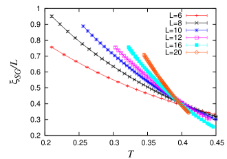
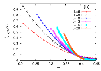
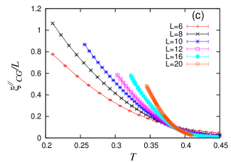
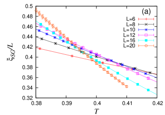
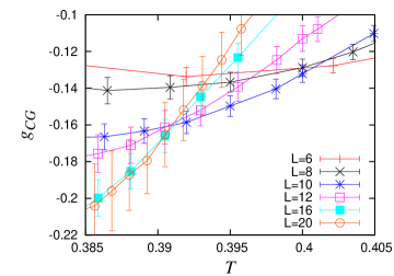
We show in Fig.1 the temperature dependence of the CG and the SG correlation-length ratios, in (a), in (b), and in (c). As can be seen from the figures, both the chiral and the spin curves cross at temperatures which are weakly -dependent. Magnified views of the crossing-temperature range are shown in Figs.2(a)-(c) for the spin, the perpendicular chirality and the parallel chirality, respectively.
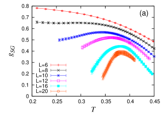
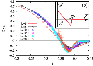
As an other indicator of the transition, we show in Fig.3 the Binder ratios for the spin (a) and for the chirality (b). The chiral Binder ratio exhibits a negative dip. The data of different cross on the negative side of . A magnified view of in the crossing-temperature region is shown in Fig.4.
In contrast to , the spin Binder ratio shown in Fig.3(a) exhibits no crossing in the investigated range of the temperature and the lattice size, monotonically decreasing with . However, develops a more and more singular shape with increasing , a prominent peak appearing for larger .
In the limit, the Binder ratios and should satisfy here in the high-temperature phase, and at . Hence, the asymptotic form of in the limit should be like the one as illustrated in the inset of Fig.3(b). In fact, such a form of is expected in a system with an ordered state exhibiting a continuous one-step-like replica-symmetry breaking (RSB) ImaKawa03b . A similar form of was observed in 3D HukuKawa05 ; VietKawamura09a ; VietKawamura09b . Note that the one-step-like RSB discussed here is of a continuous type, in contrast to the one-step RSB of a discontinuous type often discussed in conjunction with structural glasses. In the latter case, the negative dip of should exhibit a negative divergence at the transition, while such a negatively divergent behavior is not observed here.
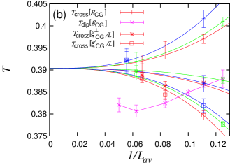
In order to estimate the bulk SG and CG transition temperatures quantitatively, we plot in Fig.5(a) the crossing temperatures of versus the inverse system size for pairs of the sizes and with and 5/4, where . Likewise, the crossing temperatures of , and are plotted versus in Fig.5(b). The crossing temperature is expected to obey the scaling form,
| (11) |
where is the correlation-length exponent and is the leading correction-to-scaling exponent. We fit our data of for the spin or for the chirality to the above form (11), to extract the transition temperature ( or ) and the exponent ( or ) for the spin or the chirality.
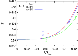
For the spin, we perform a joint fit of of for three different values of , where the values of and are taken common while the values of be -dependent. We then find an optimal fit for and with the associated value, /DOF=0.73.
For the chirality, we have several kinds of crossing temperatures , i.e., of , and . Then, we perform a joint fit of the data of of these three kinds of , each with , where and are taken common while the values of be -dependent. We then get and with the associated value, /DOF=0.51.
One sees from these results that the spin and the chiral transition temperatures agree within the error bars, i,e, within the accuracy of 1%. This observation strongly suggests the absence of the spin-chirality decoupling in 4D, in contrast to the case of 3D where lies below by about %.
For the CG transition, we have another indicator, i.e., the negative-dip temperature of the chiral Binder ratio , which is expected to obey the scaling form,
| (12) |
The data of are also shown in Fig.5(b). As can be seen from the figure, changes its behavior with increasing . It tends to decrease with for smaller sizes, while it tends to increase with for larger sizes of . Indeed, such a non-monotonic size-dependence of is expected due to the following reason. For large enough , the negative-dip temperature should lie below the crossing temperature of , . Since the exponents governing the asymptotic size dependence of and are and which satisfy the inequality by definition, needs to approach from below for large enough . Hence, a bending-up behavior observed in for larger is a necessary changeover as expected from the argument above.
Anyway, this changeover in the observed size-dependence of makes a systematic extrapolation of difficult. Nevertheless, as can be seen from Fig.5(b), our data of for larger seems fully consistent with the -value obtained above from the crossing temperatures.
As mentioned above, the negative dip of shown in Fig.3(b) is consistent with the occurrence of a one-step-like RSB HukuKawa05 ; VietKawamura09a ; VietKawamura09b . The corresponding spin Binder ratio shown in Fig.3(b) also develops a more and more singular form with a peak structure appearing for larger . If one recalls the fact that takes a value unity at and approaches zero above in the limit, is expected to develop a negative dip as in the case of . In the limit, this negative dip temperature should yield . Since is likely to agree with in 4D, a one-step-like RSB is expected to arise independently of the occurrence of the spin-chirality decoupling. In other words, in 4D, the Heisenberg SG is likely to exhibit a single SG transition without the spin-chirality decoupling. Yet, the SG (simultaneously CG) ordered state is peculiar in that the ordered state possesses a one-RSB-like nontrivial phase-space structure.
V V. Critical properties
In the previous section, we have demonstrated that, in 4D, the SG and the CG transitions are likely to take place simultaneously, i.e., . In this section, we study the critical properties of the transition on the basis of a finite-size scaling analysis of our MC data. In the absence of the spin-chirality decoupling, a natural expectation for the critical properties is that, as usual, the spin is a primary order parameter of the transition. Then one should have and . The latter corresponds to the fact that the spin is the primary order parameter and the chirality is the composite of the spin.
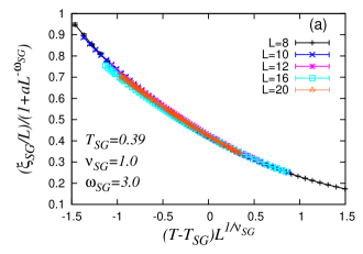
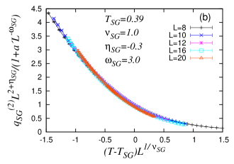
We first study the critical properties of the spin by means of a finite-size scaling analysis of both and . We employ the following finite-size scaling form with the leading correction-to-scaling term,
| (13) |
| (14) |
where and are numerical constants, while and are appropriate scaling functions. The SG transition temperature is fixed to as determined in the previous section.
We begin with the finite-size scaling of with and free fitting parameters. The best fit is obtained for and =3.0. The resulting scaling plot is given in Fig.6(a). Inspecting the quality of the plot by eyes, we put the error bars as and =3(1). Note that these estimates of and are consistent with our above estimate of . Next, with assuming and , we perform the finite-size scaling analysis of to obtain . The resulting scaling plot is shown in Fig.6(b).
We also try the type of the extended finite-size scaling analysis proposed by Campbell et al where the scaling variables are chosen to take a matching between the critical regime and the high temperature regime in order to get a wider scaling regime Campbell06 . The resulting exponent values turn out to be the same as those obtained above by the standard analysis.
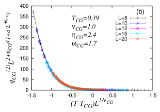
Similar scaling analysis is also applied to the chiral degrees of freedom to estimate the chiral correlation-length exponent and the chiral anomalous-dimension exponent . The transition temperature is fixed to as determined in the previous section. The finite-size scaling of the chiral correlation-length ratio yields and . We get the same estimates even when we use either the perpendicular or the transverse CG correlation-length ratio. The resulting scaling plot for the perpendicular one is given in Fig.7(a). These estimates of and are consistent with our above estimate of . The finite-size scaling of the CG order parameter with fixing and yields . The resulting scaling plot is given in Fig.7(b). We also try the extended finite-size scaling analysis a la Campbell et al Campbell06 . Again, as in the case of the spin, the resulting exponent values turn out to be the same as those obtained above by the standard analysis.

Combining the exponent estimates obtained above, we finally quote as our best estimates of the spin exponents,
| (15) |
while for the chirality exponents quote
| (16) |
If one applies the standard scaling or hyperscaling relations, one can estimate other SG exponents as , , , and , etc.
One sees from these estimates that the correlation-length exponents for the spin and for the chirality agree within the error bars, i.e., , which indicates the existence of only one diverging length scale at the transition. This observation is fully consistent with the absence of the spin-chirality decoupling in the 4D Heisenberg SG. Our data are also not incompatible with the relation within the error bars. By contrast, the anomalous-dimension exponents satisfy the inequality , indicating that the spin is the primary order parameter as usual. If one applies the scaling relation to the CG exponents , one would get the CG susceptibility exponent as . The estimated value of means that the CG susceptibility does not diverge, or diverges only weakly, at the transition. This observation is again consistent with the view that the primary order parameter in 4D is the spin and the chirality is only composite.
The obtained CG exponents values might be compared with the earlier estimates by Imagawa and Kawamura on the same model, i.e., and ImaKawa03a . One sees that agrees with our present estimate within the error bars, while deviates somewhat. In view of the larger sizes employed in the present study as compared with those of ref.ImaKawa03a , i.e., vs. , and also of larger number of independent samples, e.g., 840 vs. 80 for , our present estimate would be more trustable.
VI VI. Summary and discussion
We studied equilibrium ordering properties of the 4D isotropic Heisenberg SG by means of an extensive MC simulation. By calculating various physical quantities including the correlation-length ratio, the Binder ratio and the glass order parameter up to the size as large as and down to temperatures well below , we have found that is likely to coincide with , which indicates that the spin and the chirality order simultaneously in the 4D Heisenberg SG, i.e., the absence of the spin-chirality decoupling. If and are to differ, the distance in transition temperatures should be less than 1%. We also studied the critical properties of the transition on the basis of the finite-size scaling analysis. The exponents were estimated to be and for the spin, and and for the chirality. Although the SG transition in 4D is usual in the sense that the spin is the primary order parameter, the standard exponent relations and being satisfied. Yet, the SG transition is somewhat unusual in the sense that the low-temperature SG (simultaneously CG) ordered state exhibits a nontrivial phase-space structure, i.e., a continuous one-step-like RSB. Note that the type of RSB is quite different from the one observed in the Ising SG, or the one observed in the mean-field limit of both the Ising and the Heisenberg SGs.
As mentioned in §1, possible correspondence between the orderings of the -dimensional SR Heisenberg SG and of the 1D LR Heisenberg SG with a power-law interaction has been suggested in the literature. Although this correspondence is by no means exact, recent numerical studies both on the Ising and the Heisenberg SGs supported such correspondence. Indeed, Katzgraber et al proposed a formula for the - correspondence, a refined version of the one mentioned in §1 Katzgraber09 ,
| (17) |
where is the spin anomalous-dimension exponent of the -dimensional SR system. Now, we have an estimate of for the Heisenberg SG as . Substituting this into the r.h.s. of eq.(17) and putting , we get . Together with the recent numerical estimate of the borderline value of separating the spin-chirality coupling/decoupling regimes, VietKawamura10a ; VietKawamura10b , the - correspondence suggests that the 4D lies very close to the borderline dimensionality of the spin-chirality coupling/decoupling, on the coupling regime only slightly. Such a view on the basis of the - correspondence seems fully consistent with our present MC results.
In fact, the correspondence holds also for the critical exponents. In the - analogy, the exponent of the 1D LR model should be related to that of the -dimensional SR model via the relation, [1D-LR]=[D-SR] Larson . Then, our 4D result suggests that the corresponding 1D LR model should be characterized by the exponent . Meanwhile, ref.VietKawamura10b gave and for so that the expected relation is indeed satisfied. All these results suggest that probably lies fairly close to the borderline dimensionality of the spin-chirality decoupling/coupling, may even lie just at the border.
Acknowledgements.
The authors are thankful to T. Okubo and T. Obuchi for useful discussion. This study was supported by Grant-in-Aid for Scientific Research on Priority Areas “Novel States of Matter Induced by Frustration” (19052006 & 19052007). We thank ISSP, University of Tokyo, YITP, Kyoto University, and Cyber Media Center, Osaka University for providing us with the CPU time.References
- (1) S.F. Edwards and P.W. Anderson, J. Phys. F: Met. Phys. 5, 965 (1975).
- (2) For reviews on spin glasses, see e. g., J. A. Mydosh: Spin Glasses, (Taylor & Francis, LondonWashington DC, 1993); Spin glasses and random fields, ed. A. P. Young (World Scientific, Singapore, 1997); N. Kawashima and H. Rieger, in Frustrated Spin Systems, ed. H.T. Diep (World Scientific, Singapore, 2004).
- (3) J. R. Banavar and M. Cieplak, Phys. Rev. Lett. 48, 832 (1982).
- (4) W. L. McMillan, Phys. Rev. B. 31, 342 (1985).
- (5) J. A. Olive, A. P. Young and D. Sherrington, Phys. Rev. B 34, 6341 (1986).
- (6) F. Matsubara, T. Iyota and S. Inawashiro, Phys. Rev. Lett. 67, 1458 (1991).
- (7) H. Yoshino and H. Takayama, Europhys. Lett 22, 631 (1993).
- (8) H. Kawamura, Phys. Rev. Lett. 68, 3785 (1992).
- (9) See, for review, H. Kawamura, J. Phys. Soc. Jpn. 79, 011007 (2010); H. Kawamura, J. Phys. Conf. Ser. 233 012012 (2010).
- (10) F. Matsubara, S. Endoh and T. Shirakura, J. Phys. Soc. Jpn. 69, 1927 (2000); S. Endoh, F. Matsubara and T. Shrakura, J. Phys. Soc. Jpn. 70, 1543 (2001).
- (11) L. W. Lee and A. P. Young, Phys. Rev. Lett. 90, 227203 (2003).
- (12) I. Campos, M. Cotallo-Aban, V. Martin-Mayor, S. Perez-Gaviro and A. Tarancon, Phys. Rev. Lett. 97, 217204 (2006).
- (13) L. W. Lee and A. P. Young, Phys. Rev. B 76, 024405 (2007).
- (14) L.A. Fernandez, V. Martin-Mayor, S. Perez-Gaviro, A. Tarancon and A.P. Young, Phys. Rev. B 80, 024422 (2009).
- (15) M. Matsumoto, K. Hukushima and H. Takayama, Phys. Rev.B 66, 104404 (2002).
- (16) K. Hukushima and H. Kawamura, Phys. Rev. B 72, 144416 (2005).
- (17) I. A. Campbell and H. Kawamura, Phys. Rev. Lett. 99, 019701 (2007).
- (18) D.X. Viet and H. Kawamura, Phys. Rev. Lett. 102, 027202 (2009).
- (19) D.X. Viet and H. Kawamura, Phys. Rev. B 80, 064418 (2009).
- (20) H. Kawamura and H. Yonehara, J. Phys. A 36, 10867 (2003).
- (21) M. Weigel and M.J.P. Gingras, Phys. Rev. B 77, 104437 (2008).
- (22) D. Imagawa and H. Kawamura, Phys. Rev. B 67, 224412 (2003).
- (23) K. Binder and A.P. Young, Rev. Mod. Phys. 58, 801 (1986).
- (24) H.G. Katzgraber and A.P. Young, Phys. Rev. B 67, 134410 (2003).
- (25) H.G. Katzgraber and A.P. Young, Phys. Rev. B72, 184416 (2005).
- (26) H.G. Katzgraber, D. Larson and A.P. Young, Phys. Rev. Lett. 102, 177205 (2009).
- (27) L. Leuzzi, J. Phys. A 32, 1417 (1999).
- (28) L. Leuzzi, G. Parisi, F. Ricci-Tersenghi, and J. J. Ruiz-Lorenzo, Phys. Rev. Lett. 101, 107203 (2008).
- (29) D.X. Viet and H. Kawamura, Phys. Rev. Letters 105, 097206 (2010).
- (30) D.X. Viet and H. Kawamura, J. Phys. Soc. Jpn. 79, 104708 (2010).
- (31) A. Sharma and A.P. Young, Phys. Rev. B 83, 214405 (2011).
- (32) K. Hukushima and K. Nemoto, J. Phys. Soc. Jpn 65, 1604 (1996).
- (33) D. Imagawa and H. Kawamura, Phys. Rev. B 67, 224412 (2003).
- (34) I. A. Campbell, K. Hukushima, and H. Takayama, Phys. Rev. Lett. 97, 117202 (2006).
- (35) D. Larson, H.G. Katzgraber, M.A. Moore and A.P. Young, Phys. Rev. B 81, 064415 (2010).