Matrix Formula of Differential Resultant for First Order Generic Ordinary Differential Polynomials

Abstract: In this paper, a matrix representation for the differential resultant of two generic ordinary differential polynomials $f_{1}$ and $f_{2}$ in the differential indeterminate $y$ with order one and arbitrary degree is given. That is, a non-singular matrix is constructed such that its determinant contains the differential resultant as a factor. Furthermore, the algebraic sparse resultant of $f_{1},f_{2},\delta f_{1},\delta f_{2}$ treated as polynomials in $y,y^{\prime},y^{\prime\prime}$ is shown to be a non-zero multiple of the differential resultant of $f_{1},f_{2}$. Although very special, this seems to be the first matrix representation for a class of nonlinear generic differential polynomials.

Keywords: Matrix formula, differential resultant, sparse resultant, Macaulay resultant.

1 Introduction

Multivariate resultant, which gives a necessary condition for a set of $n+1$ polynomials in $n$ variables to have common solutions, is an important tool in elimination theory. One of the major issues in the resultant theory is to give a matrix representation for the resultant, which allows fast computation of the resultant using existing methods of determinant computation. By a matrix representation of the resultant, we mean a non-singular square matrix whose determinant contains the resultant as a factor. There exist stronger forms of matrix representations. For instance, in the case of two univariate polynomials in one variable, there exist matrix formulae named after Sylvester and B$\acute{\text{e}}$zout, whose determinants equal the resultant. Unfortunately, such determinant formulae do not generally exist for multivariate resultants. Macaulay showed that the multivariate resultant can be represented as a ratio of two determinants of certain Macaulay matrixes [15]. D’Andrea established a similar result for the multivariate sparse resultant [7] based on the pioneering work on sparse resultant [10, 16, 2]. This paper will study matrix representations for differential resultants.

Using the analogue between ordinary differential operators and univariate polynomials, the differential resultant for two linear ordinary differential operators was studied by Berkovich and Tsirulik [1] using Sylvester style matrices. The subresultant theory was first studied by Chardin [5] for two differential operators and then by Li [14] and Hong [11] for the more general Ore polynomials.

For nonlinear differential polynomials, the differential resultant is more difficult to define and study. The differential resultant for two nonlinear differential polynomials in one variable was defined by Ritt in [18, p.47]. In [22, p.46], Zwillinger proposed to define the differential resultant of two differential polynomials as the determinant of a matrix following the idea of algebraic multivariate resultant, but did not give details. General differential resultants were defined by Carrà Ferro using Macaulay’s definition of algebraic resultants [4]. But, the treatment in [4] is not complete, as will be shown in Section 2.2 of this paper. In [21], Yang, Zeng, and Zhang used the idea of algebraic Dixon resultant to compute the differential resultant. Although very efficient, this approach is not complete and does not provide a matrix representation for the differential resultant. Differential resultants for linear ordinary differential polynomials were studied by Rueda-Sendra [20]. In [19], Rueda gave a matrix representation for a generic sparse linear system. In [8], the first rigorous definition for the differential resultant of $n+1$ differential polynomials in $n$ differential indeterminates was given and its properties were proved. In [12, 13], the sparse resultant for differential Laurent polynomials was defined and a single exponential time algorithm to compute the sparse resultant was given. Note that an ideal approach is used in [8, 12, 13], and whether the multivariate differential resultant admits a matrix representation is left as an open issue.

In this paper, based on the idea of algebraic sparse resultants and Macaulay resultants, a matrix representation for the differential resultant of two generic ordinary differential polynomials $f_{1},f_{2}$ in the differential indeterminate $y$ with order one and arbitrary degree is given. The constructed square matrix has entries equal to the coefficients of $f_{1},f_{2}$, their derivatives, or zero, whose determinant is a nonzero multiple of the differential resultant. Furthermore, we prove that the sparse resultant of $f_{1},f_{2},\delta f_{1},\delta f_{2}$ treated as polynomials in $y,y^{\prime},y^{\prime\prime}$ is not zero and contains the differential resultant of $f_{1},f_{2}$ as a factor. Although very special, this seems to be the first matrix representation for a class of nonlinear generic differential polynomials.

The rest of the paper is organized as follows. In Section 2, the method of Carrà Ferro is briefly introduced and the differential resultant is defined following [8]. In Section 3, a matrix representation for the differential resultant of two differential polynomials with order one and arbitrary degree is given. In Section 4, it is shown that the differential resultant can be computed as a factor of a special algebraic sparse resultant. In Section 5, the conclusion is presented and a conjecture is proposed.

2 Preliminaries

To motivate what we do, we first briefly recall Carrà Ferro’s definition for differential resultant and then give a counter example to show the incompleteness of Carrà Ferro’s method when dealing with nonlinear generic differential polynomials. Finally, definition for differential resultant given in [8] is introduced.

2.1 A sketch of Carrà Ferro’s definition

Let $K$ be an ordinary differential field of characteristic zero with $\delta$ as a derivation operator. $K\{y\}=K[\delta^{n}y,n\in{\mathbb{N}}]$ is the differential ring of the differential polynomials in the differential indeterminate $y$ with coefficients in $K$. Let $p_{1}$ (respectively $p_{2}$) be a differential polynomial of order $m$ and degree $d_{1}$ (respectively of order $n$ and degree $d_{2}$ ) in $K\{y\}$. According to Carrà Ferro [4], the differential resultant of $p_{1},p_{2}$, denoted by $\delta\mbox{R}(p_{1},p_{2})$, is defined to be the Macaulay’s algebraic resultant of $m+n+2$ differential polynomials

$$\mathcal{P}(p_{1},p_{2})=\{\delta^{n}p_{1},\delta^{n-1}p_{1},\dots,p_{1},\delta^{m}p_{2},\delta^{m-1}p_{2},\dots,p_{2}\}$$

in the polynomial ring $S_{m+n}=K[y,\delta y,\dots,\delta^{m+n}y]$ in $m+n+1$ variables.

Specifically, let

$$D=1+(n+1)(d_{1}-1)+(m+1)(d_{2}-1),~{}~{}L={m+n+1+D\choose m+n+1}.$$

Let $y_{i}=\delta^{i}y$ for all $i=0,1,\dots,m+n$. For each $a=(a_{0},\dots,a_{m+n})\in{\mathbb{N}}^{m+n+1}$, $Y^{a}=y_{0}^{a_{0}}\cdots y_{m+n}^{a_{m+n}}$ is a power product in $S_{m+n}$. $M_{m+n+1}^{D}$ stands for the set of all power products in $S_{m+n}$ of degree less than or equal to $D$. Obviously, the cardinality of $M_{m+n+1}^{D}$ equals $L$. In a similar way it is possible to define $M_{m+n+1}^{D-d_{1}}$ which has $L_{1}={m+n+1+D-d_{1}\choose m+n+1}$ monomials, and $M_{m+n+1}^{D-d_{2}}$ which has $L_{2}={m+n+1+D-d_{2}\choose m+n+1}$ monomials. The monomials in $M_{m+n+1}^{D},M_{m+n+1}^{D-d_{1}}$ and $M_{m+n+1}^{D-d_{2}}$ are totally ordered using first the degree and then the lexicographic order derived from $y_{0}<y_{1}<\dots<y_{m+n}$.

Definition 2.1

The $(((n+1)L_{1}+(m+1)L_{2})\times L)$-matrix

$$M(\delta,n,m)=M(\delta^{n}p_{1},\dots,\delta p_{1},p_{1},\delta^{m}p_{2},\dots,\delta p_{2},p_{2}),$$

is defined in the following way: for each $i$ such that $(j-1)L_{1}<i\leq jL_{1}$ the coefficients of the polynomial $Y^{a}\delta^{n+1-j}p_{1}$ are the entries of the $i$-th row for each $Y^{a}\in M_{m+n+1}^{D-d_{1}}$ and each $j=1,\dots,n+1$, while for each $i$ such that

$$(n+1)L_{1}+(j-n-2)L_{2}<i\leq(n+1)L_{1}+(j-n-1)L_{2}$$

the coefficients of the polynomial $Y^{a}\delta^{m+n+2-j}p_{2}$ are the entries of the $i$-th row for each $Y^{a}\in M_{m+n+1}^{D-d_{2}}$ and each $j=n+2,\dots,m+n+2$, that are written with respect to the power products in $M_{m+n+1}^{D}$ in decreasing order.

Definition 2.2

The differential resultant of $p_{1}$ and $p_{2}$ is defined to be

$$\hskip 64.87224pt\gcd(\mbox{\rm{det}}(P):P~{}\mbox{is an}~{}(L\times L)\mbox{-submatrix of}~{}M(\delta,n,m)).$$

2.2 A counter example and definition of differential resultant

In this subsection, we use Carrà Ferro’s method [4] to construct matrix formula of two nonlinear generic ordinary differential polynomials with order one and degree two,

$$g_{1}=a_{0}y_{1}^{2}+a_{1}y_{1}y+a_{2}y^{2}+a_{3}y_{1}+a_{4}y+a_{5},$$

$$g_{2}=b_{0}y_{1}^{2}+b_{1}y_{1}y+b_{2}y^{2}+b_{3}y_{1}+b_{4}y+b_{5},$$ (1)

where, hereinafter, $y_{1}=\delta y$ and $a_{i},b_{i}$ with $i=0,\dots,5$ are generic differential indeterminates.

For differential polynomials in (2.2), we have $d_{1}=d_{2}=2,m=n=1$, $D=5,L=56,$ and $L_{1}=L_{2}=20$. The set of column monomials is

$$M_{3}^{5}=\{y_{2}^{5},y_{2}^{4}B_{3}^{1},y_{2}^{3}B_{3}^{2},y_{2}^{2}B_{3}^{3},y_{2}B_{3}^{4},B_{3}^{5}\},$$

where, and throughout the paper, $B=\{1,y,y_{1},y_{2}\}$ and $B_{i}^{j}$ denotes all monomials of total degree less than or equal to $j$ in the first $i$ elements of $B$. For example, $B_{2}^{2}=\{1,y,y^{2}\}$ and $B_{3}^{2}=\{1,y,y_{1},y^{2},yy_{1},y_{1}^{2}\}$. Note that the monomials of $M_{3}^{3}$ are $M_{3}^{3}=\{y_{2}^{3},y_{2}^{2}B_{3}^{1},y_{2}B_{3}^{2},B_{3}^{3}\}=B^{3}_{4}$.

According to Definition 2.1, $M(\delta,1,1)$ is an $80\times 56$ matrix

$\begin{array}[]{c}\\ \\ M_{3}^{3}\delta g_{1}\Bigg{\{}\\ \\ M_{3}^{3}g_{1}\Bigg{\{}\\ \\ M_{3}^{3}\delta g_{2}\Bigg{\{}\\ \\ M_{3}^{3}g_{2}\Bigg{\{}\\ \\ \end{array}$

$y_{2}^{5}$    $y_{2}^{4}y_{1}$    $\dots$    $y_{2}^{3}$    $\dots$        $y$      $1$

$\left(\begin{array}[]{ccccccc}0&d_{1}a_{0}&\dots&\delta a_{5}&\dots&0&0\\ &&&\dots\dots&&&\\ 0&0&\dots&0&\dots&\delta a_{4}&\delta a_{5}\\ 0&0&\dots&a_{0}&\dots&0&0\\ &&&\dots\dots&&&\\ 0&0&\dots&0&\dots&a_{4}&a_{5}\\ 0&d_{2}b_{0}&\dots&\delta b_{5}&\dots&0&0\\ &&&\dots\dots&&&\\ 0&0&\dots&0&\dots&\delta b_{4}&\delta b_{5}\\ 0&0&\dots&b_{0}&\dots&0&0\\ &&&\dots\dots&&&\\ 0&0&\dots&0&\dots&b_{4}&b_{5}\end{array}\right)$

Obviously, the entries of the first column are all zero in $M(\delta,1,1)$, since the monomial $y^{5}_{2}$ never appears in any row polynomial $Y\ast f$, where the monomial $Y\in M_{3}^{3}$ and $f\in\{\delta g_{1},g_{1},\delta g_{2},g_{2}\}$. Consequently, the differential resultant of $g_{1},g_{2}$ is identically zero according to this definition.

Actually, the differential resultant is defined using an ideal approach for two generic differential polynomials in one differential indeterminate in [18] and $n+1$ generic differential polynomials in $n$ differential indeterminates in [8]. $f$ is said to be a generic differential polynomial in differential indeterminates ${\mathbb{Y}}=\{y_{1},\dots,y_{n}\}$ with order $s$ and degree $m$ if $f$ contains all the monomials of degree up to $m$ in $y_{1},\dots,y_{n}$ and their derivatives up to order $s$. Furthermore, the coefficients of $f$ are also differential indeterminates. For instance, $g_{1}$ and $g_{2}$ in (2.2) are two generic differential polynomials.

Theorem 2.3 ([8])

Let $p_{0},p_{1},\ldots,p_{n}$ be generic differential polynomials with order $s_{i}$ and coefficient sets ${\mathbf{u}}_{i}$ respectively. Then $[p_{0},p_{1},\ldots,p_{n}]$ is a prime differential ideal in ${\mathbb{Q}}\{{\mathbb{Y}},{\mathbf{u}}_{0},$ $\ldots,{\mathbf{u}}_{n}\}$. And

$$[p_{0},p_{1},\ldots,p_{n}]\cap{\mathbb{Q}}\{{\mathbf{u}}_{0},\ldots,{\mathbf{u}}_{n}\}=\hbox{\rm{sat}}({\mathbf{R}}({\mathbf{u}}_{0},\ldots,{\mathbf{u}}_{n})).$$ (2)

is a prime differential ideal of codimension one, where ${\mathbf{R}}$ is defined to be the differential sparse resultant of $p_{0},p_{1},\ldots,p_{n}$, which has the following properties

a) ${\mathbf{R}}({\mathbf{u}}_{0},{\mathbf{u}}_{1},\ldots,{\mathbf{u}}_{n})$ is an irreducible polynomial and differentially homogeneous in each ${\mathbf{u}}_{i}$.

b) ${\mathbf{R}}({\mathbf{u}}_{0},{\mathbf{u}}_{1},\ldots,{\mathbf{u}}_{n})$ is of order $h_{i}=s-s_{i}$ in ${\mathbf{u}}_{i}$ $(i=0,\ldots,n)$ with $s=\sum_{l=0}^{n}s_{l}$.

c) The differential resultant can be written as a linear combination of $p_{i}$ and the derivatives of $p_{i}$ up to the order $s-s_{i}$. Precisely, we have

$${\mathbf{R}}({\mathbf{u}}_{0},{\mathbf{u}}_{1},\ldots,{\mathbf{u}}_{n})=\sum_{i=0}^{n}\sum_{j=0}^{s-s_{i}}h_{ij}p_{i}^{(j)}$$

where $h_{ij}\in{\mathbb{Q}}[{\mathbb{Y}},{\mathbb{Y}}^{(1)}\ldots,{\mathbb{Y}}^{(s)},{\mathbf{u}}_{0}^{(s-s_{0})},\ldots,{\mathbf{u}}_{n}^{(s-s_{n})}]$.

3 Matrix formula for differential polynomials

In this section, we will give a matrix representation for the following generic differential polynomials in $y$

$$f_{1}=a_{y_{1}^{d_{1}}}y_{1}^{d_{1}}+a_{y_{1}^{d_{1}-1}y}y_{1}^{d_{1}-1}y+\dots+a_{0},$$ (3)

$$f_{2}=b_{y_{1}^{d_{2}}}y_{1}^{d_{2}}+b_{y_{1}^{d_{2}-1}y}y_{1}^{d_{2}-1}y+\dots+b_{0},$$

where $y_{1}=\delta y$, $1\leq d_{1}\leq d_{2}$, and $a_{y_{1}^{d_{1}}},\dots,a_{0},b_{y_{1}^{d_{2}}},\dots,b_{0}$ are differential indeterminates.

3.1 Matrix construction

In this subsection, we show that when choosing a proper column monomial set, a square matrix can be constructed following Macaulay’s idea [15].

By c) of Theorem 2.3, the differential resultant for $f_{1},f_{2}$ can be written as a linear combination of $f_{1},f_{2},\delta f_{1},\delta f_{2}$ which are treated as polynomials in variables $y,y_{1},y_{2}=\delta y_{1}$. So, we will try to construct a matrix representation for the differential resultant of $f_{1},f_{2}$ from these four polynomials.

From Section 2, it is easy to see that the main problem for Carrà Ferro’s definition is that the matrix $M(\delta,n,m)$ contains too many columns. Or equivalently, the monomial set $M_{m+n+1}^{D}$ used to represent the columns is too large.

Consider the monomial set

$$\mathcal{E}=B_{3}^{D}\cup y_{2}B_{3}^{D-1}$$ (4)

with $D=2d_{1}+2d_{2}-3$. We will show that if using $\mathcal{E}$ as the column monomial set, a nonsingular square matrix can be constructed.

Define the main monomial of polynomials $p_{1}=\delta f_{1},p_{2}=\delta f_{2},p_{3}=f_{1},p_{4}=f_{2}$ to be

$$\mbox{mm}(p_{1})=y_{2}\,y_{1}^{d_{1}-1},\mbox{mm}(p_{2})=y_{1}^{d_{2}},\mbox{mm}(p_{3})=y^{d_{1}},\mbox{mm}(p_{4})=1.$$ (5)

Then, we can divide $\mathcal{E}$ into four mutually disjoint sets $\mathcal{E}={\mathcal{S}}_{1}\cup{\mathcal{S}}_{2}\cup{\mathcal{S}}_{3}\cup{\mathcal{S}}_{4}$, where

$${\mathcal{S}}_{1}=\{Y^{\alpha}\in\mathcal{E}:{\rm{mm}}(p_{1})~{}\text{divides}~{}Y^{\alpha}\},$$

$${\mathcal{S}}_{2}=\{Y^{\alpha}\in\mathcal{E}:{\rm{mm}}(p_{1})~{}\text{does not divide}~{}Y^{\alpha}~{}\text{but}~{}{\rm{mm}}(p_{2})~{}\text{does}\},$$ (6)

$${\mathcal{S}}_{3}=\{Y^{\alpha}\in\mathcal{E}:{\rm{mm}}(p_{1}),{\rm{mm}}(p_{2})~{}\text{do not divide}~{}Y^{\alpha}~{}\text{but}~{}{\rm{mm}}(p_{3})~{}\text{does}\},$$

$${\mathcal{S}}_{4}=\{Y^{\alpha}\in\mathcal{E}:{\rm{mm}}(p_{1}),{\rm{mm}}(p_{2}),{\rm{mm}}(p_{3})~{}\text{do not divide}~{}Y^{\alpha}\}.$$

As a consequence, we can write down a system of equations:

$$Y^{\alpha}/\mbox{mm}(p_{1})\ast p_{1}=0,\hskip 52.06859pt\text{for }~{}Y^{\alpha}\in{\mathcal{S}}_{1},$$

$$Y^{\alpha}/\mbox{mm}(p_{2})\ast p_{2}=0,\hskip 52.06859pt\text{for}~{}~{}Y^{\alpha}\in{\mathcal{S}}_{2},$$

$$Y^{\alpha}/\mbox{mm}(p_{3})\ast p_{3}=0,\hskip 52.06859pt\text{for }~{}Y^{\alpha}\in{\mathcal{S}}_{3},$$ (7)

$$Y^{\alpha}/\mbox{mm}(p_{4})\ast p_{4}=0,\hskip 52.06859pt\text{for }~{}Y^{\alpha}\in{\mathcal{S}}_{4}.$$

Observe that the total number of equations is the number of elements in $\mathcal{E}$ and denoted by $N=(D+1)^{2}$.

Regarding the monomials in (3.1) as unknowns, we obtain a system of $N$ linear equations about these monomial unknowns. Denote the coefficient matrix of the system of linear equations (3.1) by $D_{d_{1},d_{2}}$ whose elements are zero or the coefficients of $f_{i}$ and $\delta f_{i},i=1,2$.

Note that the main monomials of the polynomials are not the maximal monomials in the sense of Macaulay [15], so the monomials on the left hand side of (3.1) may not be contained in $\mathcal{E}$. Next, we prove that this does not occur for our main monomials.

Lemma 3.1

The coefficient matrix $D_{d_{1},d_{2}}$ of system (3.1) is square.

Proof: The coefficient matrix of system (3.1) has $N=|\mathcal{E}|$ rows. In order to prove the lemma, it suffices to demonstrate that, for each $Y^{\alpha}\in{\mathcal{S}}_{i},i=1,\ldots,4$, all monomials in $[Y^{\alpha}/\mbox{mm}(p_{i})]\ast p_{i}$ are contained in $\mathcal{E}$. Recall that $\mathcal{E}=B_{3}^{D}\cup y_{2}B_{3}^{D-1}$. Then by (3.1), one has

$${\mathcal{S}}_{1}=B_{3}^{D-d_{1}}\ast\mbox{mm}(p_{1})=B_{3}^{D-d_{1}}\ast\mbox{mm}(\delta f_{1}),$$

$${\mathcal{S}}_{2}=B_{3}^{D-d_{2}}\ast\mbox{mm}(p_{2})=B_{3}^{D-d_{2}}\ast\mbox{mm}(\delta f_{2}),$$

$${\mathcal{S}}_{3}=T_{1}\ast\mbox{mm}(p_{3})=T_{1}\ast\mbox{mm}(f_{1}),$$ (8)

$${\mathcal{S}}_{4}=T_{2}\ast\mbox{mm}(p_{4})=T_{2}\ast\mbox{mm}(f_{2}),$$

where

$$T_{1}=\left\{\Big{(}\bigcup_{i=0}^{d_{2}-1}y_{1}^{i}B_{2}^{D-d_{1}-i}\Big{)}\bigcup\Big{(}y_{2}\bigcup_{i=0}^{d_{1}-2}y_{1}^{i}B_{2}^{D-d_{1}-1-i}\Big{)}\right\},$$ (9)

$$T_{2}=\left\{\Big{(}\bigcup_{i=0}^{d_{2}-1}y_{1}^{i}B_{2}^{d_{1}-1}\Big{)}\bigcup\Big{(}y_{2}\bigcup_{i=0}^{d_{1}-2}y_{1}^{i}B_{2}^{d_{1}-1}\Big{)}\right\}.$$

Note that the representation of ${\mathcal{S}}_{2}$ in (3.1) is obtained with the help of the condition $d_{1}\leq d_{2}$.

Hence, the equations (3.1) become

$$B_{3}^{D-d_{1}}\ast\delta f_{1}=0,$$

$$B_{3}^{D-d_{2}}\ast\delta f_{2}=0,$$ (10)

$$T_{1}\ast f_{1}=0,$$

$$T_{2}\ast f_{2}=0.$$

Since the monomial set of $\delta f_{1}$ is $B_{3}^{d_{1}}\cup y_{2}\ast B_{3}^{d_{1}-1}$, the monomial set of $B_{3}^{D-d_{1}}\ast\delta f_{1}$ is $B_{3}^{D-d_{1}}\ast(B_{3}^{d_{1}}\cup y_{2}\ast B_{3}^{d_{1}-1})=B_{3}^{D}\cup y_{2}B_{3}^{D-1}=\mathcal{E}$. So monomials in the first set of equations in (10) are in $\mathcal{E}$. Since the monomial set of $f_{1}$ is $B_{3}^{d_{1}}=\cup_{l=0}^{d_{1}}y_{1}^{l}B_{2}^{d_{1}-l}$, the monomial set of $T_{1}\ast f_{1}$ is $T_{11}\cup y_{2}T_{12}$, where $T_{11}=\bigcup_{k=0}^{d_{1}+d_{2}-1}y_{1}^{k}B_{2}^{D-k}$ and $T_{12}=\bigcup_{k=0}^{2d_{1}-2}y_{1}^{k}B_{2}^{D-k-1}$. Since $d_{1}\geq 1$ and $d_{2}\geq 1$, we have $d_{1}+d_{2}-1\leq D=2d_{1}+2d_{2}-3$ and hence $T_{11}\subset B_{3}^{D}$. Since $d_{1}\geq 1$ and $d_{2}\geq 1$, we have $2d_{1}-2\leq D-1=2d_{1}+2d_{2}-4$ and hence $T_{12}\subset B_{3}^{D-1}$. As a consequence, $T_{11}\cup y_{2}T_{12}\subset\mathcal{E}$ and the monomials in the third set of equations in (10) are in $\mathcal{E}$. Other cases can be proved similarly. Thus all monomials in the left hand side of (10) are in $\mathcal{E}$. This proves the lemma. $\Box$

It is worthy to say that, due to the decrease of the number of monomials in $\mathcal{E}$ compared with the method by Carrà Ferro, the size of the matrix $D_{d_{1},d_{2}}$ decreases significantly.

3.2 Matrix representation for differential resultant

In this section, we show that $\mbox{det}(D_{d_{1},d_{2}})$ is not identically equal to zero and contains the differential resultant as a factor.

Lemma 3.2

$\hbox{\rm{det}}(D_{d_{1},d_{2}})$ is not identically equal to zero.

Proof: It suffices to show that there exists a unique monomial in the sense that it is different from all other monomials in the expansion of $\mbox{det}(D_{d_{1},d_{2}})$.

The coefficients of the main monomials in $\delta f_{1},\delta f_{2},f_{1},f_{2}$ are respectively

$$\delta f_{1}:~{}~{}a_{y_{1}^{d_{1}}}\hskip 81.09052pt\mbox{the coefficient of}~{}\mbox{mm}(\delta f_{1})=y_{2}y_{1}^{d_{1}-1},$$

$$\delta f_{2}:~{}~{}\delta b_{y_{1}^{d_{2}}}+b_{y_{1}^{d_{2}-1}y}\hskip 31.2982pt\mbox{the coefficient of}~{}\mbox{mm}(\delta f_{2})=y_{1}^{d_{2}},$$ (11)

$$f_{1}~{}:~{}~{}a_{y^{d_{1}}}\hskip 82.51282pt\mbox{the coefficient of}~{}\mbox{mm}(f_{1})=y^{d_{1}},$$

$$f_{2}~{}:~{}~{}b_{0}\hskip 92.47145pt\mbox{the coefficient of}~{}\mbox{mm}(f_{2})=1.$$

We will show that the monomial $(a_{y_{1}^{d_{1}}})^{n_{1}}(\delta b_{y_{1}^{d_{2}}})^{n_{2}}(a_{y^{d_{1}}})^{n_{3}}(b_{0})^{n_{4}}$ is a unique one by the following four steps, where $n_{i}$ is the number of elements in ${\mathcal{S}}_{i}$ with $i=1,\dots,4$. From (10), $n_{1}=|B_{3}^{D-d_{1}}|$, $n_{2}=|B_{3}^{D-d_{2}}|$, $n_{3}=|T_{1}|$, $n_{4}=|T_{2}|$.

1. Observe that, in $\delta f_{1}$, $a_{y^{d_{1}}}$ only occurs in the coefficient of $y_{1}y^{d_{1}-1}$ with the form $a_{y^{d_{1}}}+\delta a_{y_{1}y^{d_{1}-1}}$. Furthermore, $\delta a_{y_{1}y^{d_{1}-1}}$ only occurs in this term given by $\delta f_{1}$ and no other places of $D_{d_{1},d_{2}}$. So using the transformation

$$\delta a_{y_{1}y^{d_{1}-1}}=c_{y_{1}y^{d_{1}-1}}-d_{1}a_{y^{d_{1}}},~{}~{}\mbox{with other coefficients unchanged, }$$ (12)

where $c_{y_{1}y^{d_{1}-1}}$ is a new differential indeterminate, $D_{d_{1},d_{2}}$ is transformed to a new matrix which is singular if and only if the original one is singular. Still denote the matrix by $D_{d_{1},d_{2}}$.

From (10), for a monomial $M\in T_{1}$, $a_{y^{d_{1}}}$ is the coefficient of the monomial $My^{d_{1}}$ in each polynomial $T_{1}\ast f_{1}$ and hence in each corresponding row of $D_{d_{1},d_{2}}$. Then $a_{y^{d_{1}}}$ is in different rows and columns of $D_{d_{1},d_{2}}$, and this gives the factor $(a_{y^{d_{1}}})^{n_{3}}$. Delete those rows and columns of $D_{d_{1},d_{2}}$ containing $a_{y^{d_{1}}}$ and denote the remaining matrix by $D^{(1)}_{d_{1},d_{2}}$. From (10), the columns deleted are represented by monomials $y^{d_{1}}T_{1}$. So, $D^{(1)}_{d_{1},d_{2}}$ is still a square matrix.

2. Let $M\in B_{3}^{D-d_{1}}$. The term $a_{y_{1}^{d_{1}}}$ occurs in $M\ast\delta f_{1}$ as the coefficient of the monomial $y_{2}y_{1}^{d_{1}-1}M$, or equivalently it occurs in the columns represented by $y_{2}y_{1}^{d_{1}-1}M$. This gives the factor $(a_{y_{1}^{d_{1}}})^{n_{1}}$. It is easy to check that $a_{y_{1}^{d_{1}}}$ does not occur in other places of $D^{(1)}_{d_{1},d_{2}}$. From the definition for $T_{1}$ (9), the columns deleted in case 1 correspond those columns represented by monomials of the form $y_{2}^{k_{2}}y_{1}^{k_{1}}y^{d_{1}}$ where either $k_{2}=0$ and $k_{1}<d_{2}$ or $k_{2}=1$ and $k_{1}<d_{1}-1$. Then $\{y^{d_{1}}T_{1}\}\cap\{y_{2}y_{1}^{d_{1}-1}B_{3}^{D-d_{1}}\}=\emptyset$, or equivalently those columns of $D_{d_{1},d_{2}}$ containing $a_{y_{1}^{d_{1}}}$ are still in $D^{(1)}_{d_{1},d_{2}}$. Similar to case 1, one can delete those rows and columns of $D^{(1)}_{d_{1},d_{2}}$ containing $a_{y_{1}^{d_{1}}}$ and denote the remaining matrix by $D^{(2)}_{d_{1},d_{2}}$ which is still a square matrix. From (10), the columns deleted are represented by monomials $y_{2}y_{1}^{d_{1}-1}B_{3}^{D-d_{1}}$.

3. At the moment, $D^{(2)}_{d_{1},d_{2}}$ only contains coefficients of $f_{2}$ and $\delta f_{2}$. Observe that $b_{0}$ only occurs in the rows corresponding to $T_{2}\ast f_{2}$, where $T_{2}$ is defined in (9). Note that $\delta b_{0}$ instead of $b_{0}$ occurs in $\delta f_{2}$. Since $\{y^{d_{1}}T_{1}\}\cap T_{2}=\emptyset$ and $\{y_{2}y_{1}^{d_{1}-1}B_{3}^{D-d_{1}}\}\cap T_{2}=\emptyset$, the columns of $D_{d_{1},d_{2}}$ containing $b_{0}$, represented by $T_{2}$, are not deleted in case 1 and case 2. Then, we have the factor $(b_{0})^{n_{4}}$. Similarly, delete those rows and columns of $D^{(2)}_{d_{1},d_{2}}$ containing $b_{0}$ and denote the remaining matrix by $D^{(3)}_{d_{1},d_{2}}$ which is still a square matrix. From (10), the columns deleted are represented by monomials $T_{2}$.

4. From (10), the rows of $D^{(3)}_{d_{1},d_{2}}$ are from coefficients of $B_{3}^{D-d_{2}}\ast\delta f_{2}$. The term $\delta b_{y_{1}^{d_{2}}}$ is in the coefficient of the monomial $M\ast y_{1}^{d_{2}}$ in $M\ast\delta f_{2}$ for $M\in B_{3}^{D-d_{2}}$, and $\delta b_{y_{1}^{d_{2}}}$ does not occur in other places of $M\ast\delta f_{2}$. Furthermore, since $\{y^{d_{1}}T_{1}\}\cap\{y_{1}^{d_{2}}B_{3}^{D-d_{2}}\}=\emptyset$, $\{y_{2}y_{1}^{d_{1}-1}B_{3}^{D-d_{1}}\}\cap\{y_{1}^{d_{2}}B_{3}^{D-d_{2}}\}=\emptyset$, and $T_{2}\cap\{y_{1}^{d_{2}}B_{3}^{D-d_{2}}\}\}=\emptyset$, the columns containing the term $\delta b_{y_{1}^{d_{2}}}$ are not deleted in the first three cases. Then, we have the factor $(\delta b_{y_{1}^{d_{2}}})^{n_{2}}$.

Following the above procedures step by step, the coefficients of choosing main monomials of the polynomials $f_{1},f_{2},\delta f_{1},\delta f_{2}$ occur in each row and each column of $D_{d_{1},d_{2}}$ and only once, and the monomial $\big{(}a_{y_{1}^{d_{1}}}\big{)}^{n_{1}}\big{(}\delta b_{y_{1}^{d_{2}}}\big{)}^{n_{2}}\big{(}a_{y^{d_{1}}}\big{)}^{n_{3}}\big{(}b_{0}\big{)}^{n_{4}}$ is a unique one in the expansion of the determinant of $D_{d_{1},d_{2}}$. So the lemma follows. $\Box$

Note that the selection of main monomials in above algorithm is not unique, thus there may exist other ways to construct matrix formula for system (3).

Corollary 3.3

Following the above notations, for any $Y^{\alpha}\in{\mathcal{S}}_{i}$, if all monomials of $[Y^{\alpha}/\text{mm}(p_{j})]*p_{j}$ are contained in $\mathcal{E}(j\neq i)$, then the rearranged matrix, which is obtained by replacing the row polynomials $[Y^{\alpha}/\text{mm}(p_{i})]*p_{i}$ by $[Y^{\alpha}/\text{mm}(p_{j})]*p_{j}$, is not identically equal to zero.

Corollary 3.3 follows from the fact that the proof of Lemma 3.2 is independent of the number of elements in ${\mathcal{S}}_{i}$ as long as the main monomials are the same.

The relation between $\mbox{det}(D_{d_{1},d_{2}})$ and differential resultant of $f_{1},f_{2}$, denoted by ${\mathbf{R}}$, is stated as the following theorem.

Theorem 3.4

$\mbox{\rm{det}}(D_{d_{1},d_{2}})$ is a nonzero multiple of ${\mathbf{R}}$.

Proof. From Lemma 3.2, $\det(D_{d_{1},d_{2}})$ is nonzero. In the matrix $D_{d_{1},d_{2}}$, multiply a column monomial $M\neq 1$ in ${\mathcal{E}}$ to the corresponding column and add the result to the constant column corresponding to the monomial $1$. Then the constant column becomes $Y^{\alpha}\ast p_{i}$ with $p_{1}=\delta f_{1},p_{2}=\delta f_{2},p_{3}=f_{1},p_{4}=f_{2}$ and $Y^{\alpha}\in{\mathcal{S}}_{i}/\mbox{mm}(p_{i})$, $i=1,\dots,4$. Since a determinant is multi-linear on the columns, expanding the matrix by the constant column, we obtain

$$\mbox{det}(D_{d_{1},d_{2}})=h_{1}\,f_{1}+h_{2}\,\delta f_{1}+h_{3}\,f_{2}+h_{4}\,\delta f_{2},$$ (13)

where $h_{j}$ are differential polynomials. From (2), $\mbox{det}(D_{d_{1},d_{2}})\in\mbox{sat}({\mathbf{R}})$. On the other hand, from Theorem 2.3, ${\mathbf{R}}$ is irreducible and the order of ${\mathbf{R}}$ about the coefficients of $f_{1},f_{2}$ is one. Therefore, ${\mathbf{R}}$ must divide $\mbox{det}(D_{d_{1},d_{2}})$.$\Box$

From Theorem 3.4, we can easily deduce a degree bound $N=4(d_{1}+d_{2}-1)^{2}$ for the differential resultant of $f_{1}$ and $f_{2}$. The main advantage to represent the differential resultant as a factor of the determinant of a matrix is that we can use fast algorithms of matrix computation to compute the differential resultant as did in the algebraic case [3].

Suppose that $\mbox{det}(D_{d_{1},d_{2}})$ is expanded as a polynomial. Then the differential resultant can be found by the following result.

Corollary 3.5

Suppose $\mbox{\rm{det}}(D_{d_{1},d_{2}})=\prod_{i=1}^{s}P_{i}^{e_{i}}$ is an irreducible factorization of $\mbox{det}(D_{d_{1},d_{2}})$ in ${\mathbb{Q}}[C_{f_{1}},C_{f_{2}}]$, where $C_{f_{i}},i=1,2$ are the sets of coefficients of $f_{i}$. Then there exists a unique factor, say $P_{1}$, which is in $[f_{1},f_{2}]$ and is the differential resultant of $f_{1}$ and $f_{2}$.

Proof. From c) of Theorem 2.3 and Theorem 3.4, ${\mathbf{R}}\in[f_{1},f_{2}]$ and is an irreducible factor of $\mbox{det}(D_{d_{1},d_{2}})$. Suppose $\mbox{det}(D_{d_{1},d_{2}})$ contains another factor, say $P_{2}$, which is also in $[f_{1},f_{2}]$. Then $P_{2}\in\mbox{sat}({\mathbf{R}})$ by (2). Since ${\mathbf{R}}$ is irreducible with order one and $P_{2}$ is of order no more than one, $P_{2}$ must equal ${\mathbf{R}}$, which contradicts to the hypothesis.$\Box$

3.3 Example (2.2) revisited

In this section, we apply the method just proposed to construct a matrix representation for the differential resultant of the system (2.2).

Following the method given in the proceeding section, for system (2.2), we have $D=2d_{1}+2d_{2}-3=5$ and select the main monomials of $\delta g_{1},\delta g_{2},g_{1},g_{2}$ are $y_{2}y_{1},y_{1}^{2},y^{2},1$ respectively. Then $\mathcal{E}=y_{2}B_{3}^{4}\cup B_{3}^{5}$ is divided into the following four disjoint sets

$${\mathcal{S}}_{1}=y_{2}y_{1}B_{3}^{3},$$

$${\mathcal{S}}_{2}=y_{1}^{2}B_{3}^{3},$$

$${\mathcal{S}}_{3}=y^{2}\left[B_{2}^{3}\cup y_{1}B_{2}^{2}\cup y_{2}B_{2}^{2}\right],$$ (14)

$${\mathcal{S}}_{4}=B_{2}^{1}\cup y_{1}B_{2}^{1}\cup y_{2}B_{2}^{1}.$$

Using (3.1) and regarding the monomials in $\mathcal{E}$ as variables, we obtain the matrix $D_{2,2}$, which is a $36\times 36$ square matrix in the following form.

$\begin{array}[]{r}\\ \\ B_{3}^{3}\delta g_{1}\Bigg{\{}\\ \\ (B_{2}^{3}\cup y_{1}B_{2}^{2}\cup y_{2}B_{2}^{2})g_{1}\Bigg{\{}\\ \\ B_{3}^{3}\delta g_{2}\Bigg{\{}\\ \\ (B_{2}^{1}\cup y_{1}B_{2}^{1}\cup y_{2}B_{2}^{1})g_{2}\Bigg{\{}\\ \\ \end{array}$

$y_{2}y_{1}^{4}$   $y_{2}y_{1}^{3}y$  $\dots$  $y_{2}y_{1}^{2}y^{2}$  $\dots$    $y$      $1$

$\left(\begin{array}[]{ccccccc}2a_{0}&a_{1}&\dots&0&\dots&0&0\\ &&&\dots\dots&&&\\ 0&0&\dots&0&\dots&\delta a_{4}&\delta a_{5}\\ 0&0&\dots&a_{0}&\dots&0&0\\ &&&\dots\dots&&&\\ 0&0&\dots&0&\dots&a_{4}&a_{5}\\ 2b_{0}&b_{1}&\dots&0&\dots&0&0\\ &&&\dots\dots&&&\\ 0&0&\dots&0&\dots&\delta b_{4}&\delta b_{5}\\ 0&0&\dots&b_{0}&\dots&0&0\\ &&&\dots\dots&&&\\ 0&0&\dots&0&\dots&b_{4}&b_{5}\end{array}\right)$

As shown in the proof of Lemma 3.2, $(a_{0})^{10}(a_{2})^{10}(b_{5})^{6}(\delta b_{0})^{10}$ is a unique monomial in the expansion of the determinant of $D_{2,2}$. Hence, the differential resultant of $g_{1}$ and $g_{2}$ is a factor of $\mbox{det}(D_{2,2})$. Note that in Carrà Ferro’s construction for $g_{1},g_{2}$, $M(\delta,1,1)$ is an $80\times 56$ matrix, which is larger than $D_{2,2}$.

In particular, suppose $a_{0}=b_{0}=1$ and $a_{i},b_{i}$ are differential constants, i.e, $\delta a_{i}=\delta b_{i}=0$, $i=1,\dots,5$. Then $D_{2,2}$ can be expanded as a polynomial and the differential resultant of $g_{1},g_{2}$ can be found with Corollary 3.5, which is a polynomial of degree 12 and contains 3210 terms. This is the same as the result obtained in [21].

4 Differential resultant as the algebraic sparse resultant

In this section, we show that differential resultant of $f_{1}$ and $f_{2}$ is a factor of the algebraic sparse resultant of the system $\{f_{1},f_{2},\delta f_{1},\delta f_{2}\}$.

4.1 Results about algebraic sparse resultant

In this subsection, notions of algebraic sparse resultants are introduced. Detailed can be found in [3, 6, 10, 16].

A set $S$ in $\mathbbm{R}^{n}$ is said to be convex if it contains the line segment connecting any two points in $S$. If a set is not itself convex, its convex hull is the smallest convex set containing it and denoted by Conv($S$). A set $V=\{a_{1},\ldots,a_{m}\}$ is called a vertex set of a convex set $Q$ if each point $q\in Q$ can be expressed as

$$q=\sum_{j=1}^{m}\lambda_{j}a_{j},~{}~{}~{}~{}\text{with}~{}\sum_{j=1}^{m}\lambda_{j}=1~{}\text{and}~{}\lambda_{j}\geq 0,$$

and each $a_{j}$ is called a vertex of $Q$.

Consider $n+1$ generic sparse polynomials in the algebraic indeterminates $x_{1},\dots,x_{n}$:

$$p_{i}=u_{i0}+u_{i1}M_{i1}+\cdots+u_{il_{i}}M_{il_{i}},~{}~{}~{}i=1,\ldots,n+1,$$

where $u_{ij}$ are indeterminates and $M_{ik}=\prod_{s=1}^{n}x_{s}^{e^{ik_{s}}}$ are monomials in ${\mathbb{Q}}[x_{1},\ldots,x_{n}]$ with exponent vectors $a_{ik}=(e^{ik_{1}},\ldots,e^{ik_{n}})\in\mathbbm{Z}^{n}$. Note that we assume each $p_{i}$ contains a constant term $u_{i0}$. For $a=(e^{1},\ldots,e^{n})\in\mathbbm{Z}^{n}$, the corresponding monomial is denoted as $M(a)=\prod_{s=1}^{n}x_{s}^{e^{s}}$.

The finite set $\mathcal{A}_{i}\subset\mathbbm{Z}^{n}$ of all monomial exponents appearing in $p_{i}$ is called the support of $p_{i}$, denoted by supp($p_{i}$). Its cardinality is $l_{i}=|\mathcal{A}_{i}|$. The Newton polytope $Q_{i}\subset\mathbbm{R}^{n}$ of $p_{i}$ is the convex hull of $\mathcal{A}_{i}$, denoted by $Q_{i}={\rm Conv}(\mathcal{A}_{i})$. Since $Q_{i}$ is the convex hull for a finite set of points, it must have a vertex set. For simplicity, we assume that each $\mathcal{A}_{i}$ is of dimension $n$ as did in [10, p.252]. Let ${\mathbf{u}}$ be the set of coefficients of $p_{i},i=0,\ldots,n$. Then, the ideal

$$(p_{1},p_{2},\ldots,p_{n+1})\cap{\mathbb{Q}}[{\mathbf{u}}]=(\SS({\mathbf{u}}))$$ (15)

is principal and the generator $\SS$ is defined to be the sparse resultant of $p_{1},\ldots,p_{n+1}$ [10, p.252]. When the coefficients ${\mathbf{u}}$ of $p_{i}$ are specialized to certain values ${\mathbf{v}}$, the sparse resultant for the specialized polynomials is defined to be $\SS({\mathbf{v}})$. The matrix representation of $\SS$ is associated with the decomposition of the Minkowski sum of the Newton polytopes $Q_{i}$.

The Minkowski sum of the convex polytopes $Q_{i}$

$$Q=Q_{1}+\dots+Q_{n+1}=\{q_{1}+\dots+q_{n+1}|q_{i}\in Q_{i}\}.$$

is still convex and of dimension $n$.

Choose sufficiently small numbers $\delta_{i}>0$ and let $\delta=(\delta_{1},\ldots,\delta_{n})\in{\mathbbm{R}}^{n}$ be a perturbed vector. Then the points which lie in the interior of the perturbed district ${\mathcal{E}}=\mathbb{Z}^{n}\cap(Q+\delta)$ are chosen as the column monomial set [3] to construct the matrix for the sparse resultant.

Choose $n+1$ sufficiently generic linear lifting functions $l_{1},\dots,l_{n+1}\in\mathbb{Z}[x_{1},\dots,x_{n}]$ and define the lifted Newton polytopes $\widehat{Q}_{i}=\{\widehat{q}_{i}=(q_{i},l_{i}(q_{i})):q_{i}\in Q_{i}\}\subset\mathbb{R}^{n+1}$. Let

$$\widehat{Q}=\sum_{i=1}^{n+1}\widehat{Q}_{i}\subset\mathbb{R}^{n+1}$$

which is an $(n+1)$-dimensional convex polytope. The lower envelope of $\widehat{Q}$ with respect to vector $(0,\dots,0,1)\in\mathbb{R}^{n+1}$ is the union of all the $n$-dimensional faces of $\widehat{Q}$, whose inner normal vector has positive last component.

Let $\pi:(q_{1},\dots,q_{n+1})\mapsto(q_{1},\dots,q_{n})$ be the projection to the first $n$ coordinates from $\mathbb{R}^{n+1}$ to $\mathbb{R}^{n}$. Then $\pi$ is a one to one map between the lower envelope of $\widehat{Q}$ and $Q$ [3]. The genericity requirements on $l_{i}$ assure that every point $\widehat{q}$ on the lower envelope can be uniquely expressed as $\widehat{q}=\widehat{q}_{1}+\dots+\widehat{q}_{n+1}$ with $\widehat{q}_{i}\in\widehat{Q}_{i}$, such that the sum of the projections under $\pi$ of these points leads to a unique sum of $q=q_{1}+\dots+q_{n+1}\in Q\subset\mathbb{R}^{n}$ with $q_{i}\in Q_{i}$, which is called the optimal (Minkowski) sum of $q$. For $\mathcal{F}_{i}\subset Q_{i}$, $R=\sum_{i=1}^{n+1}\mathcal{F}_{i}$ is called an optimal sum, if each element of $R$ can be written as a unique optimal sum $\sum_{i=0}^{n}p_{i}$ for $p_{i}\in\mathcal{F}_{i}$.

A polyhedral subdivision of an $n$-dimensional polytope $Q$ consists of finitely many $n$-dimensional polytopes $R_{1},\dots,R_{s}$, called the cells of the subdivision, such that $Q=R_{1}\cup\dots\cup R_{s}$ and for $i\neq j$ and $R_{i}\cap R_{j}$ is either empty or a face of both $R_{i}$ and $R_{j}$. A polyhedral subdivision is called a mixed subdivision if each cell $R_{l}$ can be written as an optimal sum $R_{l}=\sum_{i=1}^{n+1}\mathcal{F}_{i}$, where each $\mathcal{F}_{i}$ is a face of $Q_{i}$ and $n=\sum_{i=1}^{n+1}\text{dim}(\mathcal{F}_{i})$. Furthermore, if $R_{j}=\sum_{i=1}^{n+1}\mathcal{F}^{\prime}_{i}$ is another cell in the subdivision, then $R_{l}\cap R_{j}=\sum_{i=1}^{n+1}(\mathcal{F}_{i}\cap\mathcal{F}^{\prime}_{i})$. A cell $R_{l}=\sum_{i=1}^{n+1}\mathcal{F}_{i}$ is called mixed if dim($\mathcal{F}_{i})\leq 1$ for all $i$; otherwise, it is a non-mixed cell. As a result of $n=\sum_{i=1}^{n+1}\text{dim}(\mathcal{F}_{i})$, a mixed cell has one unique vertex, which satisfies $\text{dim}(\mathcal{F}_{i_{0}})=0$, while a non-mixed cell has at least two vertices.

Recall $\delta=(\delta_{1},\delta_{2},\ldots,\delta_{n})$, where $0<\delta_{i}<1$. If $Q=R_{1}\cup\dots\cup R_{s}$ is a subdivision of $Q$, then $\delta+Q=(\delta+R_{1})\cup\dots\cup(\delta+R_{s})$ is a subdivision of $\delta+Q$.

Let $q\in\mathbb{Z}^{n}\cap(Q+\delta)$ lie in the interior of a cell $\delta+\mathcal{F}_{1}+\dots+\mathcal{F}_{n+1}$ of a mixed subdivision for $Q+\delta$, where $\mathcal{F}_{i}$ is a face of $Q_{i}$. The row content function of $q$ is defined as the largest integer such that $\mathcal{F}_{i}$ is a vertex. In fact, all the vertices in the optimal sum of $p$ can be selected as the row content functions. Hence, we define generalized row content functions (GRC for brief) as one of the integers, not necessary largest, such that $\mathcal{F}_{i}$ is a vertex.

Suppose that we have a mixed subdivision of $Q$. With a fixed GRC, a sparse resultant matrix can be constructed as follows. For each $i=1,\ldots,n+1$, define the subset $S_{i}$ of $\mathcal{E}$ as follows:

$$S_{i}=\{q\in{\mathcal{E}}\,|\,\hbox{GRC}(q)=(i,j_{0})\},$$ (16)

where $j_{0}\in\{1,\dots,m_{i}\}$, $m_{i}$ is the number of vertexes of $Q_{i}$, and we obtain a disjoint union for $\mathcal{E}$:

$$\mathcal{E}=S_{1}\cup\cdots\cup S_{n+1}.$$ (17)

For $q\in S_{i}$, let $q=q_{1}+\dots+q_{n+1}\in Q$ be an optimal sum of $q$. Then, $q_{i}$ is a vertex of $Q_{i}$ and the corresponding monomial $M(q_{i})$ is called the main monomial of $p_{i}$ and denoted by ${\rm{mm}}(p_{i})$, similar to what we did in Section 3. Main monomials have the following important property [6, p350].

Lemma 4.1

If $q\in S_{i}$, then the monomials in $(M(q)/{\rm{mm}}(p_{i}))p_{i}$ are contained in ${\mathcal{E}}$.

Now consider the following equation systems

$$(M(q)/{\rm{mm}}(p_{i}))p_{i},~{}~{}~{}~{}q\in S_{i},i=1,\ldots,n+1.$$ (18)

Treating the monomials in ${\mathcal{E}}$ as variables, by Lemma 4.1, the coefficient matrix for the equations in (18) is an $|{\mathcal{E}}|\times|{\mathcal{E}}|$ square matrix, called the sparse resultant matrix. The sparse resultant of $p_{i},i=1,\ldots,n+1$ is a factor of the determinant of this matrix.

In [2, 3], Canny and Emiris used linear programming algorithms to find the row content functions and to construct $S_{i}$. We briefly describe this procedure below.

Now assume $Q_{i}$ has the vertex set $V_{i}=\{a_{i1},\dots,a_{i\,m_{i}}\}$. A point $q\in\mathbb{Z}^{n}\cap(Q+\delta)$ implies that $q\in\sigma+\delta$ with a cell $\sigma\in Q$. In order to obtain the generalized row content functions of $q$, we wish to find the optimal sum of $q-\delta$ in terms of the vertexes in $V_{i}$. Introducing variables $\lambda_{ij},i=1,\ldots,n+1,j=1,\ldots,m_{i}$, one has

$$q-\delta=\sum_{i=1}^{n+1}q_{i}=\sum_{i=1}^{n+1}\sum_{j=1}^{m_{i}}\lambda_{ij}~{}a_{ij},~{}~{}~{}~{}\text{with}~{}\sum_{j=1}^{m_{i}}\lambda_{ij}=1~{}\text{and}~{}\lambda_{ij}\geq 0.$$ (19)

On the other hand, in order to make the lifted points lie on the lower envelope of $\widehat{Q}$, one must force the “height” of the listed points minimal, thus requiring to find $\lambda_{ij}$ such that

$$\sum_{i=1}^{n+1}\sum_{j=1}^{m_{i}}\lambda_{ij}~{}l_{i}(a_{ij})~{}~{}~{}~{}\text{to be minimized}$$ (20)

under the linear constraint conditions (19), where $l_{i}(a_{ij})$ is a random linear function in $a_{ij}$.

For $q\in{\mathcal{E}}$, let $\lambda_{ij}^{*}$ be an optimal solution for the linear programming problem (20). Then $q-\delta=\sum_{i=1}^{n+1}q_{i}^{*}$ where $q_{i}^{*}=\sum_{j=1}^{m_{i}}\lambda_{ij}^{*}l_{i}(a_{ij})$. $a_{ij_{0}}^{*}$ is a vertex of $Q_{i}$ if and only if there exists a $j_{0}$ such that $\lambda_{ij_{0}}^{*}=1$ and $\lambda_{ij}^{*}=0$ for $j\neq j_{0}$. In this case, the generalized row content function of $q$ is $(i,j_{0})$ and ${\rm{mm}}(p_{i})$ is $M(a_{ij_{0}}^{*})$. It is shown that when the lift functions $l_{i}$ are general enough, all $S_{i}$ can be computed in the above way [3].

In order to study the linear programming problem (20), we need to recall a lemma about the optimality criterion for the general linear programming problem

$$\min_{x}~{}~{}~{}~{}~{}~{}~{}z=c^{T}x$$

$$\text{subject to}~{}~{}~{}~{}~{}Ax=b,~{}~{}\text{with}~{}~{}l\leq x\leq u,$$ (21)

where $A$ is an $m\times n$ rectangular matrix, $b$ is a column vector of dimension $m$, $c$ and $x$ are column vectors of dimension $n$, and the superscript $T$ stands for transpose. In order for the linear programming problem to be meaningful, the row rank of $A$ must be less than the column rank of $A$. We thus can assume $A$ to be row full rank. Let $n_{1},\ldots,n_{m}$ be linear independent columns of $A$. Then the corresponding $x_{n_{1}},\ldots,x_{n_{m}}$ are called basic variables of $x$. Let $B$ be the matrix consisting of the $n_{1},\ldots,n_{m}$ columns of $A$. Then $B$ is an $m\times m$ invertible matrix. Lemma 4.2 below gives an optimality criterion for the linear programming problem (4.1).

Lemma 4.2

([9]) Let $x_{B}$ be a basic variables set of $x$, where $B$ is the corresponding coefficient matrix of $x_{B}$. If the corresponding basic feasible solution $x_{B}=B^{-1}b\geq 0$ and the conditions $c_{B}B^{-1}A-c\leq 0$ hold, where $c_{B}$ is the row vector obtained by listing the coefficients of $x_{B}$ in the object function, then an optimal solution for the linear programming problem (4.1) can be given as $x_{B}=B^{-1}b$ and all other $x_{i}$ equals zero, which is called the optimal solution determined by the basic variables $x_{B}$.

4.2 Algebraic sparse resultant matrix

In this subsection, we show that the sparse resultant for $f_{1},f_{2},\delta f_{1},\delta f_{2}$ is nonzero and contains the differential resultant of $f_{1}$ and $f_{2}$ as a factor.

For the differential polynomials $f_{1}$ and $f_{2}$ given in (3), consider the $p_{1}=\delta f_{1},p_{2}=\delta f_{2},p_{3}=f_{1},p_{4}=f_{2}$ as algebraic polynomials in $y,y_{1},y_{2}$. The monomial sets of $\delta f_{1},\delta f_{2},f_{1},f_{2}$ are $B_{3}^{d_{1}}\cup y_{2}\ast B_{3}^{d_{1}-1}$, $B_{3}^{d_{2}}\cup y_{2}\ast B_{3}^{d_{2}-1}$, $B_{3}^{d_{1}}$, and $B_{3}^{d_{2}}$ respectively. For convenience, we will not distinguish a monomial $M$ and its exponential vector when there exists no confusion. Then the Newton polytopes for $\delta f_{1},\delta f_{2},f_{1},f_{2}$ are respectively,

$$Q_{1}=\mbox{Conv}({\rm{sup}}(\delta f_{1}))=\mbox{Conv}(B_{3}^{d_{1}}\cup y_{2}\ast B_{3}^{d_{1}-1})\subset{\mathbbm{R}}^{3},$$

$$Q_{2}=\mbox{Conv}({\rm{sup}}(\delta f_{2}))=\mbox{Conv}(B_{3}^{d_{2}}\cup y_{2}\ast B_{3}^{d_{2}-1})\subset{\mathbbm{R}}^{3},$$

$$Q_{3}=\mbox{Conv}({\rm{sup}}(f_{1}))=\mbox{Conv}(B_{3}^{d_{1}})\subset{\mathbbm{R}}^{3},$$ (22)

$$Q_{4}=\mbox{Conv}({\rm{sup}}(f_{2}))=\mbox{Conv}(B_{3}^{d_{2}})\subset{\mathbbm{R}}^{3},$$

The Newton polytopes $Q_{1}$ and $Q_{3}$ are shown in Figure 1 (for $d_{1}=5$) while $Q_{2}$ and $Q_{4}$ have similar polytopes as $Q_{1}$ and $Q_{3}$ but with different sizes respectively.

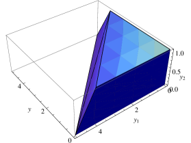
Figure 1: The Newton polytopes $Q_{1}$ and $Q_{3}$

Let the Minkowski sum $Q=Q_{1}+Q_{2}+Q_{3}+Q_{4}$. In order to compute the column monomial set, we choose a perturbed vector $\delta=(\delta_{1},\delta_{2},\delta_{3})$ with $0<\delta_{i}<1$ with $i=1,2,3$. Then the points in $\mathbb{Z}^{3}\cap(Q+\delta)$ is easily shown to be $yy_{1}y_{2}\mathcal{E}$ where ${\mathcal{E}}$ is given in (4). Note that using ${\mathcal{E}}$ or $yy_{1}y_{2}\mathcal{E}$ as the column monomial set will lead to the same matrix.

The vertex sets of $Q_{i}$, denoted by $\mbox{V}_{i}$, are respectively

$$\mbox{V}_{1}:=\{(0,0,0),(0,0,1),(0,d_{1}-1,1),(0,d_{1},0),(d_{1}-1,0,1),(d_{1},0,0)\},$$

$$\mbox{V}_{2}:=\{(0,0,0),(0,0,1),(0,d_{2}-1,1),(0,d_{2},0),(d_{2}-1,0,1),(d_{2},0,0)\},$$

$$\mbox{V}_{3}:=\{(0,0,0),(0,d_{1},0),(d_{1},0,0)\},$$

$$\mbox{V}_{4}:=\{(0,0,0),(0,d_{2},0),(d_{2},0,0)\}.$$

Let the lifting functions be $l_{i}=(L_{i1},L_{i2},L_{i3}),i=1,\dots,4$, where $L_{ij}$ are parameters to be determined later. From (20), the object function of the linear programming problem to be solved is

$$\min_{\lambda_{ij}}(\lambda_{12}L_{13}+\lambda_{13}[L_{12}(d_{1}-1)+L_{13}]+\lambda_{14}L_{12}d_{1}+\lambda_{15}[L_{11}(d_{1}-1)+L_{13}]+\lambda_{16}L_{11}d_{1}$$

$$+\lambda_{22}L_{23}+\lambda_{23}[L_{22}(d_{2}-1)+L_{23}]+\lambda_{24}L_{22}d_{2}+\lambda_{25}[L_{21}(d_{2}-1)+L_{23}]+\lambda_{26}L_{21}d_{2}$$

$$+\lambda_{32}L_{32}d_{1}+\lambda_{33}L_{31}d_{1}$$ (23)

$$+\lambda_{42}L_{42}d_{2}+\lambda_{43}L_{41}d_{2})$$

under the constraints

$$A_{1}=\lambda_{15}(d_{1}-1)+\lambda_{16}d_{1}+\lambda_{25}(d_{2}-1)+\lambda_{26}d_{2}+\lambda_{33}d_{1}+\lambda_{43}d_{2},$$

$$A_{2}=\lambda_{13}(d_{1}-1)+\lambda_{14}d_{1}+\lambda_{23}(d_{2}-1)+\lambda_{24}d_{2}+\lambda_{32}d_{1}+\lambda_{42}d_{2},$$

$$A_{3}=\lambda_{12}+\lambda_{13}+\lambda_{15}+\lambda_{22}+\lambda_{23}+\lambda_{25},$$ (24)

$$\sum_{j=1}^{m_{i}}\lambda_{ij}=1,~{}i=1,\dots,4,$$

$$\lambda_{ij}\geq 0,i=1,\ldots,4,j=1,\ldots,m_{i}~{}~{}\text{with}~{}m_{1}=m_{2}=6,m_{3}=m_{4}=3,$$

where $A_{1}=\varepsilon_{1}-\delta_{1},A_{2}=\varepsilon_{2}-\delta_{2},A_{3}=\varepsilon_{3}-\delta_{3}$ with $(\varepsilon_{1},\varepsilon_{2},\varepsilon_{3})\in\mathbb{Z}^{3}\cap(Q+\delta)$. According to the procedure given in Section 4.1, we need to solve the linear programming problem (4.2) for each $(\varepsilon_{1},\varepsilon_{2},\varepsilon_{3})\in\mathbb{Z}^{n}\cap(Q+\delta)$. Note that $L_{ij}$ are parameters. What we need to do is to show that there exist $L_{ij}$ such that the solutions of (4.2) make the corresponding main monomials to be the ones selected by us in (5). More precisely, we need to determine $L_{ij}$ such that for each $q\in\mathbb{Z}^{n}\cap(Q+\delta)$, the optimal solution for the linear programming problem (4.2) consists one of the following cases:

$$\lambda_{13}=1\hbox{ implies }\hbox{GRC}(q)=(1,3),\hbox{ the vertex is }(0,d_{1}-1,1),\hbox{ and }{\rm{mm}}(\delta f_{1})=y_{2}y_{1}^{d_{1}-1},$$

$$\lambda_{24}=1\hbox{ implies }\hbox{GRC}(q)=(2,4),\hbox{ the vertex is }(0,d_{2},0),\hbox{ and }{\rm{mm}}(\delta f_{2})=y_{1}^{d_{2}},$$

$$\lambda_{33}=1\hbox{ implies }\hbox{GRC}(q)=(3,3),\hbox{ the vertex is }(d_{1},0,0),\hbox{ and }{\rm{mm}}(f_{1})=y^{d_{1}},$$

$$\lambda_{41}=1\hbox{ implies }\hbox{GRC}(q)=(4,1),\hbox{ the vertex is }(0,0,0),\hbox{ and }{\rm{mm}}(f_{2})=1.$$

The following lemma proves that the above statement is valid.

Lemma 4.3

There exist $L_{ij}$ such that the optimal solution of the corresponding linear programming problem (4.2) can be chosen such that the corresponding main monomials for $f_{1},f_{2},\delta f_{1},\delta f_{2}$ are $\text{mm}(f_{1})=y^{d_{1}}$, $\text{mm}(f_{2})=1$, $\text{mm}(\delta f_{1})=y_{2}y_{1}^{d_{1}-1}$, $\text{mm}(\delta f_{2})=y_{1}^{d_{2}}$ respectively and ${\mathcal{E}}$ can be written as a disjoint union ${\mathcal{E}}=S_{1}\cup S_{2}\cup S_{3}\cup S_{4}$, where $S_{i}$ is defined in (16).

Proof. We write the linear programming problem as the standard form (4.1). It is easy to see

$$c=(0,L_{13},(d_{1}-1)L_{12}+L_{13},d_{1}L_{12},(d_{1}-1)L_{11}+L_{13},d_{1}L_{11},$$

$$\hskip 23.61583pt0,L_{23},(d_{2}-1)L_{22}+L_{23},d_{2}L_{22},(d_{2}-1)L_{21}+L_{23},d_{2}L_{21},$$

$$\hskip 23.61583pt0,d_{1}L_{32},d_{1}L_{31},0,d_{2}L_{42},d_{2}L_{41}).$$

Let $\delta=(\delta_{1},\delta_{2},\delta_{3})$ be a sufficiently small vector in sufficiently generic position, the validity of $\delta$ is analyzed in [3]. Then

A=$\left(\begin{array}[]{cccccccccccccccccc}0&0&0&0&\widetilde{d}_{1}&d_{1}&0&0&0&0&\widetilde{d}_{2}&d_{2}&0&0&d_{1}&0&0&d_{2}\\ 0&0&\widetilde{d}_{1}&d_{1}&0&0&0&0&\widetilde{d}_{2}&d_{2}&0&0&0&d_{1}&0&0&d_{2}&0\\ 0&1&1&0&1&0&0&1&1&0&1&0&0&0&0&0&0&0\\ 1&1&1&1&1&1&0&0&0&0&0&0&0&0&0&0&0&0\\ 0&0&0&0&0&0&1&1&1&1&1&1&0&0&0&0&0&0\\ 0&0&0&0&0&0&0&0&0&0&0&0&1&1&1&0&0&0\\ 0&0&0&0&0&0&0&0&0&0&0&0&0&0&0&1&1&1\end{array}\right),$

where $\widetilde{d}_{1}=d_{1}-1,\widetilde{d}_{2}=d_{2}-1$, which is a $7\times 18$ matrix and $b=(A_{1},A_{2},A_{3},1,1,1,1)$. It is easy to see that the rank of $A$ is 7, since $d_{1}\geq 1$.

From (4), we have ${\mathcal{E}}=\mathbb{Z}^{3}\cap(Q+\delta)=yy_{1}y_{2}(B_{3}^{D}\cup y_{2}B_{3}^{D-1})$, where $D=2d_{1}+2d_{2}-3$. We will construct a disjoint union ${\mathcal{E}}=S_{1}\cup S_{2}\cup S_{3}\cup S_{4}$ like (17) such that the corresponding main monomials are respectively $\text{mm}(\delta f_{1})=y_{2}y_{1}^{d_{1}-1}$, $\text{mm}(\delta f_{2})=y_{1}^{d_{1}}$,$\text{mm}(f_{1})=y^{d_{1}}$, $\text{mm}(f_{2})=1$.

Four cases will be considered.

Case 1. We will give the conditions about $L_{ij}$ under which $\text{mm}(\delta f_{1})=y_{2}y_{1}^{d_{1}-1}$, or equivalently, the linear programming problem (4.2) has an optimal solution where $\lambda_{13}=1$. As a consequence, $S_{1}$ will also be constructed.

As shown by Lemma 4.2, an optimal solution for a linear programming problem can be uniquely determined by a set of basic variables. We will construct the required optimal solutions by choosing different sets of basic variables. Four sub-cases are considered.

1.1. Selecting basic variables as $\text{vet}_{11}=\{\lambda_{13},\lambda_{23},\lambda_{24},\lambda_{32},\lambda_{33},\lambda_{41},\lambda_{43}\}$ while other variables are nonbasic variables and equal to zero. Due the constraint $\lambda_{11}+\lambda_{12}+\dots+\lambda_{16}=1$, we have $\lambda_{13}=1$. Then for any such an optimal solution of the linear programming problem (4.2), in the optimal sum of any element $q=q_{1}+q_{2}+q_{3}+q_{4}$, $q_{1}=(0,d_{1}-1,1)$ is a vertex of $Q_{1}$, $\text{mm}(\delta f_{1})=y_{2}y_{1}^{d_{1}-1}$, and the corresponding $q$ belongs to $S_{1}$ as defined in (16).

We claim that the basic feasible solutions in $\text{vet}_{11}$ must be nondegenerate meaning that all basic variables are positive, that is, $x_{B}=B^{-1}b>0$. A mixed cell $R=\sum_{i=1}^{4}\mathcal{F}_{i}$, where $\mathcal{F}_{i}$ is a face of $Q_{i}$, must satisfy the dimension constraint $\sum_{i=1}^{4}\dim(\mathcal{F}_{i})=3$. In the cell corresponding to the basic variables $\text{vet}_{11}$, ${\mathcal{F}}_{1}=(0,d_{1}-1,1)$ is a vertex of $Q_{1}$, ${\mathcal{F}}_{4}$ is a one dimensional face of $Q_{4}$ of the form $\lambda_{41}V_{41}+\lambda_{43}V_{43}$, where $V_{41}=(0,0,0)$, $V_{43}=(d_{2},0,0)$, and $\lambda_{41}+\lambda_{43}=1$. ${\mathcal{F}}_{2}$ and ${\mathcal{F}}_{3}$ are one dimensional faces of $Q_{2}$ and $Q_{3}$ respectively. In order for the dimension constraint $\sum_{i=1}^{4}\dim(\mathcal{F}_{i})=3$ to be valid, the claim must be true. For otherwise, one of the variables in $\text{vet}_{11}$ must be zero, say $\lambda_{41}=0$. Then $\lambda_{43}=1$ and ${\mathcal{F}}_{4}$ becomes a vertex, which implies $\sum_{i=1}^{4}\dim(\mathcal{F}_{i})<3$, a contradiction.

From Lemma 4.2, the coefficient matrix of basic variables in (4.2) is

$B_{{11}}=\left(\begin{array}[]{ccccccc}0&0&0&0&d_{1}&0&d_{2}\\ d_{1}-1&d_{2}-1&d_{2}&d_{1}&0&0&0\\ 1&1&0&0&0&0&0\\ 1&0&0&0&0&0&0\\ 0&1&1&0&0&0&0\\ 0&0&0&1&1&0&0\\ 0&0&0&0&0&1&1\end{array}\right),$

with rank($B_{{11}}$)=7. For all $(A_{1},A_{2},A_{3})$ and $b=(A_{1},A_{2},A_{3},1,1,1,1)$, the requirement $B_{{11}}^{-1}b>0$ in Lemma 4.2 gives

$$1<A_{3}<2,d_{1}+d_{2}<A_{2}+A_{3}<2d_{1}+d_{2},$$

$$2d_{1}+d_{2}<A_{1}+A_{2}+A_{3}<2d_{1}+2d_{2}.$$

Substituting $A_{1}=\varepsilon_{1}-\delta_{1},A_{2}=\varepsilon_{2}-\delta_{2},A_{3}=\varepsilon_{3}-\delta_{3}$ into the above inequalities and considering that $(\varepsilon_{1},\varepsilon_{2},\varepsilon_{3})$ are integer points, we have

$$\varepsilon_{3}=2,~{}~{}\varepsilon_{2}=d_{1}+d_{2}-1,\dots,2d_{1}+d_{2}-2,$$ (25)

$$\varepsilon_{1}+\varepsilon_{2}=2d_{1}+d_{2}-1,\dots,2d_{1}+2d_{2}-2.$$

On the other hand, $c_{B_{{}_{11}}}=((d_{1}-1)L_{12}+L_{13},(d_{2}-1)L_{22}+L_{23},d_{2}L_{22},d_{1}L_{32},d_{1}L_{31},0,$ $d_{2}L_{41})$. After simplification and rearrangement, the condition $c_{B_{{}_{11}}}B_{{}_{11}}^{-1}A-c\leq 0$ in Lemma 4.2 becomes

$$\{L_{12}-L_{11}+L_{31}-L_{32},L_{12}+L_{31}-L_{32}-L_{41},$$

$$\hskip 5.69046ptL_{13}-L_{12}+L_{22}-L_{23},L_{22}-L_{21}+L_{31}-L_{32},$$ (26)

$$\hskip 5.69046ptL_{22}+L_{31}-L_{32}-L_{41},L_{31}-L_{41},L_{32}-L_{31}+L_{41}-L_{42}\}\leq 0$$

where, hereinafter, $\{w_{1},\dots,w_{s}\}\leq 0$ means $w_{i}\leq 0$ for $i=1,\dots,s$.

By Lemma 4.2, if (25) and (4.2) are valid, we obtain an optimal solution of the linear programming problem (4.2) which is determined by the basic variables $\text{vet}_{11}$. Hence, if (4.2) is valid, the corresponding $q=(\varepsilon_{1},\varepsilon_{2},\varepsilon_{3})$ in and (25) are in $S_{1}$, since in the optimal decomposition of $q=q_{1}+q_{2}+q_{3}+q_{4}$, $q_{1}=(0,d_{1}-1,1)$ is a vertex.

1.2. Similarly, choosing the basic variables as $\text{vet}_{12}=\{\lambda_{13},\lambda_{23},\lambda_{24},\lambda_{31},\lambda_{32},\lambda_{33},\lambda_{41}\}$, which generates a new basic matrix $B_{{12}}$, and from $B_{{12}}^{-1}b>0$, we obtain

$$0<A_{1},d_{1}+d_{2}<A_{2}+A_{3},1<A_{3}<2,A_{1}+A_{2}+A_{3}<2d_{1}+d_{2},$$

which in turn lead to the following values for $\varepsilon_{1},\varepsilon_{2},\varepsilon_{3}$

$$\varepsilon_{3}=2,~{}~{}\varepsilon_{1}=1,\dots,~{}~{}\varepsilon_{2}=d_{1}+d_{2}-1,\dots,$$ (27)

$$\varepsilon_{1}+\varepsilon_{2}=d_{1}+d_{2},\dots,2d_{1}+d_{2}-2.$$

The condition $c_{B_{{12}}}B_{{12}}^{-1}A-c\leq 0$ leads to the following constraints on $L_{ij},i=1,\dots,4,j=1,2,3$,

$$\{L_{12}-L_{11}+L_{31}-L_{32},L_{12}-L_{32},$$

$$\hskip 5.69046ptL_{13}-L_{12}+L_{22}-L_{23},L_{22}-L_{32},$$ (28)

$$\hskip 5.69046ptL_{22}-L_{21}+L_{31}-L_{32},L_{31}-L_{41},L_{32}-L_{42}\}\leq 0.$$

1.3. Similarly, the basic variables $\text{vet}_{13}=\{\lambda_{13},\lambda_{23},\lambda_{24},\lambda_{32},\lambda_{33},\lambda_{41},$ $\lambda_{42}\}$ lead to

$$\varepsilon_{3}=2,~{}~{}\varepsilon_{1}=1,\dots,d_{1},~{}~{}$$

$$\varepsilon_{1}+\varepsilon_{2}=2d_{1}+d_{2}-1,\dots,2d_{1}+2d_{2}-2,$$ (29)

and

$$\{L_{12}-L_{42},L_{12}-L_{11}+L_{31}-L_{32},$$

$$\hskip 5.69046ptL_{13}-L_{12}+L_{22}-L_{23},L_{22}-L_{21}+L_{31}-L_{32},$$ (30)

$$\hskip 5.69046ptL_{22}-L_{42},L_{31}-L_{32}-L_{41}+L_{42},L_{32}-L_{42}\}\leq 0.$$

1.4. Similarly, the basic variables $\text{vet}_{14}=\{\lambda_{13},\lambda_{23},\lambda_{24},\lambda_{33},\lambda_{41},\lambda_{42},$ $\lambda_{43}\}$ lead to

$$\varepsilon_{3}=2,~{}~{}\varepsilon_{1}=d_{1}+1,\dots,~{}~{}\varepsilon_{2}=d_{1}+d_{2}-1,\dots,$$

$$\varepsilon_{1}+\varepsilon_{2}=2d_{1}+d_{2},\dots,2d_{1}+2d_{2}-2.$$ (31)

and

$$\{L_{12}-L_{11}+L_{41}-L_{42},L_{12}-L_{42},$$

$$\hskip 5.69046ptL_{13}-L_{12}+L_{22}-L_{23},L_{22}-L_{21}+L_{41}-L_{42},$$ (32)

$$\hskip 5.69046ptL_{22}-L_{42},L_{31}-L_{41},L_{31}-L_{32}-L_{41}+L_{42}\}\leq 0.$$

Let $S_{1}$ be the set $(\varepsilon_{1},\varepsilon_{2},\varepsilon_{3})$ defined in (25), (27), (4.2), and (4.2). Then for $\eta\in S_{1}$ and an optimal sum of $\eta=q_{1}+q_{2}+q_{3}+q_{4}$, since $\lambda_{13}=1$, $q_{1}$ must be the vertex $(0,d_{1}-1,1)$ of $Q_{1}$. Therefore, $\text{mm}(\delta f_{1})=y_{2}y_{1}^{d_{1}-1}$. Of course, in order for this statement to be valid, $L_{ij}$ must satisfy constraints (4.2), (4.2), (4.2), and (4.2). We will show later that these constraints indeed have common solutions.

The following three cases can be treated similarly, and we only list the conditions for $\varepsilon_{1},\varepsilon_{2},\varepsilon_{3}$ while the concrete requirements for $L_{ij}$ are listed at the end of the proof.

Case 2. In order for $\text{mm}(\delta f_{2})=y_{1}^{d_{1}}$, we choose the basic variables

$$\text{vet}_{21}=\{\lambda_{13},\lambda_{14},\lambda_{24},\lambda_{31},\lambda_{32},\lambda_{33},\lambda_{41}\},$$

$$\text{vet}_{22}=\{\lambda_{13},\lambda_{14},\lambda_{24},\lambda_{33},\lambda_{41},\lambda_{42},\lambda_{43}\},$$

$$\text{vet}_{23}=\{\lambda_{13},\lambda_{14},\lambda_{24},\lambda_{32},\lambda_{33},\lambda_{41},\lambda_{43}\},$$

$$\text{vet}_{24}=\{\lambda_{13},\lambda_{14},\lambda_{24},\lambda_{32},\lambda_{33},\lambda_{41},\lambda_{42}\},$$

$$\text{vet}_{25}=\{\lambda_{11},\lambda_{12},\lambda_{13},\lambda_{24},\lambda_{31},\lambda_{33},\lambda_{41}\},$$

$$\text{vet}_{26}=\{\lambda_{13},\lambda_{14},\lambda_{15},\lambda_{24},\lambda_{33},\lambda_{41},\lambda_{43}\},$$

$$\text{vet}_{27}=\{\lambda_{12},\lambda_{13},\lambda_{14},\lambda_{15},\lambda_{24},\lambda_{33},\lambda_{41}\},$$

which lead to the following elements of $S_{2}$

$$\varepsilon_{3}=1,~{}~{}0<\varepsilon_{1},~{}~{}d_{1}+d_{2}-1<\varepsilon_{2},\varepsilon_{1}+\varepsilon_{2}=d_{1}+d_{2}+1,\dots,2d_{1}+d_{2}-1;$$

$$\varepsilon_{3}=1,~{}~{}d_{1}<\varepsilon_{1},~{}~{}d_{1}+d_{2}-1<\varepsilon_{2},\varepsilon_{1}+\varepsilon_{2}=2d_{1}+d_{2}+1,\dots,2d_{1}+2d_{2}-1;$$

$$\varepsilon_{3}=1,~{}~{}\varepsilon_{2}=d_{1}+d_{2},\dots,2d_{1}+d_{2}-1,~{}~{}\varepsilon_{1}+\varepsilon_{2}=2d_{1}+d_{2},\dots,2d_{1}+2d_{2}-1;$$

$$\varepsilon_{3}=1,~{}~{}\varepsilon_{1}=1,\dots,d_{1},~{}~{}\varepsilon_{1}+\varepsilon_{2}=2d_{1}+d_{2},\dots,2d_{1}+2d_{2}-1;$$

$$\varepsilon_{3}=1,~{}~{}\varepsilon_{1}=1,\dots,d_{1},~{}~{}\varepsilon_{2}=d_{2}+1,\dots,d_{1}+d_{2}-1;$$

$$\varepsilon_{3}=1,~{}~{}\varepsilon_{2}=d_{2}+1,\dots,d_{1}+d_{2}-1,~{}~{}\varepsilon_{2}=2d_{1}+d_{2},\dots,2d_{1}+2d_{2}-1;$$

$$\varepsilon_{3}=1,~{}~{}\varepsilon_{1}=d_{1}+1,\dots,~{}~{}\varepsilon_{2}=d_{2}+1,\dots,\varepsilon_{1}+\varepsilon_{2}=d_{1}+d_{2}+2,\dots,2d_{1}+d_{2}-1.$$

Case 3. In order for $\text{mm}(f_{1})=y_{1}^{d_{1}}$, we choose the basic variables

$$\text{vet}_{31}=\{\lambda_{15},\lambda_{16},\lambda_{24},\lambda_{26},\lambda_{33},\lambda_{41},\lambda_{43}\},$$

$$\text{vet}_{32}=\{\lambda_{13},\lambda_{15},\lambda_{23},\lambda_{24},\lambda_{33},\lambda_{41},\lambda_{43}\},$$

$$\text{vet}_{33}=\{\lambda_{15},\lambda_{23},\lambda_{24},\lambda_{25},\lambda_{33},\lambda_{41},\lambda_{43}\},$$

$$\text{vet}_{34}=\{\lambda_{12},\lambda_{13},\lambda_{15},\lambda_{23},\lambda_{24},\lambda_{33},\lambda_{41}\},$$

which lead to the following results about $\varepsilon_{1},\varepsilon_{2},\varepsilon_{3}$ in $S_{3}$

$$\varepsilon_{3}=1,~{}~{}\varepsilon_{2}=1,\dots,d_{2},~{}~{}\varepsilon_{1}+\varepsilon_{2}=2d_{1}+d_{2},\dots,2d_{1}+2d_{2}-1;$$

$$\varepsilon_{3}=2,~{}~{}\varepsilon_{2}=d_{2},\dots,d_{1}+d_{2}-2,\varepsilon_{1}+\varepsilon_{2}=2d_{1}+d_{2}-1,\ldots,2d_{1}+2d_{2}-2;$$ (33)

$$\varepsilon_{3}=2,~{}~{}\varepsilon_{2}=1,\dots,d_{2}-1,~{}~{}\varepsilon_{1}+\varepsilon_{2}=2d_{1}+d_{2}-1,\dots,2d_{1}+2d_{2}-2;$$

$$\varepsilon_{3}=2,~{}~{}\varepsilon_{1}=d_{1}+1,\dots,~{}~{}\varepsilon_{2}=d_{2},\dots,\varepsilon_{1}+\varepsilon_{2}=d_{1}+d_{2}+1,\dots,2d_{1}+d_{2}-2.$$

Case 4. In order for ${\rm{mm}}(f_{2})=1$, we choose the following basic variables

$$\text{vet}_{41}=\{\lambda_{11},\lambda_{12},\lambda_{21},\lambda_{24},\lambda_{26},\lambda_{31},\lambda_{41}\},$$

$$\text{vet}_{42}=\{\lambda_{11},\lambda_{12},\lambda_{24},\lambda_{26},\lambda_{31},\lambda_{33},\lambda_{41}\},$$

$$\text{vet}_{43}=\{\lambda_{11},\lambda_{12},\lambda_{15},\lambda_{24},\lambda_{26},\lambda_{33},\lambda_{41}\},$$

$$\text{vet}_{44}=\{\lambda_{12},\lambda_{13},\lambda_{23},\lambda_{24},\lambda_{31},\lambda_{33},\lambda_{41}\},$$

$$\text{vet}_{45}=\{\lambda_{12},\lambda_{23},\lambda_{24},\lambda_{25},\lambda_{31},\lambda_{33},\lambda_{41}\},$$

$$\text{vet}_{46}=\{\lambda_{12},\lambda_{21},\lambda_{22},\lambda_{23},\lambda_{25},\lambda_{31},\lambda_{41}\},$$

$$\text{vet}_{47}=\{\lambda_{12},\lambda_{15},\lambda_{23},\lambda_{25},\lambda_{26},\lambda_{33},\lambda_{41}\},$$

which correspond to the elements in $S_{4}$

$$\varepsilon_{3}=1,~{}~{}0<\varepsilon_{1},~{}~{}0<\varepsilon_{2},~{}~{}\varepsilon_{1}+\varepsilon_{2}=2,\dots,d_{2};$$

$$\varepsilon_{3}=1,~{}~{}\varepsilon_{2}=1,\dots,d_{2},~{}~{}\varepsilon_{1}+\varepsilon_{2}=d_{2}+1,\dots,d_{1}+d_{2};$$

$$\varepsilon_{3}=1,~{}~{}\varepsilon_{2}=1,\dots,d_{2},~{}~{}\varepsilon_{1}+\varepsilon_{2}=d_{1}+d_{2}+1,\dots,2d_{1}+d_{2}-1;$$

$$\varepsilon_{3}=2,~{}~{}\varepsilon_{1}=1,\dots,d_{1},~{}~{}\varepsilon_{2}=d_{2},\dots,d_{1}+d_{2}-2;$$

$$\varepsilon_{3}=2,~{}~{}\varepsilon_{2}=1,\dots,d_{2}-1,~{}~{}\varepsilon_{1}+\varepsilon_{2}=d_{2},\dots,d_{1}+d_{2}-1;$$

$$\varepsilon_{3}=2,~{}~{}\varepsilon_{1}=1,\dots,~{}~{}\varepsilon_{2}=1,\dots,d_{2}-2,~{}~{}\varepsilon_{1}+\varepsilon_{2}=2,\dots,d_{2}-1;$$

$$\varepsilon_{3}=1,~{}~{}\varepsilon_{2}=1,\dots,d_{2}-1,\varepsilon_{1}+\varepsilon_{2}=d_{1}+d_{2}-1,\dots,2d_{1}+d_{2}-2.$$

Merge all the constraints for $L_{ij}$, we obtain

$$L_{11}-L_{12}-L_{21}+L_{22}\leq 0,$$

$$L_{13}\leq L_{23},L_{21}\leq L_{31}\leq L_{11}\leq L_{41},$$ (34)

$$L_{22}\leq L_{12}\leq L_{32}\leq L_{42},L_{31}=L_{32}+L_{41}-L_{42}.$$

The solution set for system (4.2) is nonempty. For example, $l_{1}=(7,-4,-5),l_{2}=(5,-9,5),l_{3}=(6,2,1),l_{4}=(8,4,7)$, which will be used for example (2.2), satisfy the conditions in (4.2).

We can also check that ${\mathcal{E}}=S_{1}\cup S_{2}\cup S_{3}\cup S_{4}$ is a disjoint union for ${\mathcal{E}}$. The lemma is proved.$\Box$

We now have the main result of this section.

Theorem 4.4

The sparse resultant of $f_{1},f_{2},\delta f_{1},\delta f_{2}$ as polynomials in $y,y_{1},y_{2}$ is not identically zero and contains the differential resultant of $f_{1}$ and $f_{2}$ as a factor.

Proof. Note that $a_{0},b_{0},\delta a_{0},\delta b_{0}$, which are the zero degree terms of $f_{1}$, $f_{2}$, $\delta f_{1}$, $\delta f_{2}$ respectively, are algebraic indeterminates. As a consequence,

$$J_{1}=(f_{1},f_{2},\delta f_{1},\delta f_{2})$$

is a prime ideal in ${\mathbb{Q}}[{\mathbf{u}},y,y_{1},y_{2}]$, where ${\mathbf{u}}$ is the set of the coefficients of $f_{1},f_{2}$ are their first order derivatives. Let

$$J_{2}=J_{1}\cap{\mathbb{Q}}[{\mathbf{u}}].$$

Then $J_{2}$ is also a prime ideal. We claim that

$$J_{2}=({\mathbf{R}})$$ (35)

where ${\mathbf{R}}$ is the differential resultant of $f_{1},f_{2}$. From c) of Theorem 2.3, ${\mathbf{R}}\in J_{2}$. Let $T\in J_{2}$. Then $T\in J_{1}\subset[f_{1},f_{2}]$. From (2), the pseudo remainder of $T$ with respect to ${\mathbf{R}}$ is zero. Also note that the order of $T$ in $a_{i},b_{i}$ is less than or equal to $1$. From a) and b) of Theorem 2.3, ${\mathbf{R}}$ must be a factor of $T$, which proves (35).

From Lemma 4.3, the main monomials for $f_{1},f_{2},\delta f_{1},\delta f_{2}$ are the same as those used to construct ${\mathcal{S}}_{1},{\mathcal{S}}_{2},{\mathcal{S}}_{3},{\mathcal{S}}_{4}$ in (5). As a consequence, we have $S_{1}\subset{\mathcal{S}}_{1}$. For $q\in{\mathcal{S}}_{1}\setminus S_{1}$, $q$ must be in some $S_{i}$, say $q\in S_{2}$. Then from Lemma 4.3, the monomials in $(M(q)/{\rm{mm}}(\delta f_{2}))\delta f_{2}$ are contained in ${\mathcal{E}}$. By Corollary 3.3, the sparse resultant matrix of $f_{1},f_{2},\delta f_{1},\delta f_{2}$ obtained after move $q$ from $S_{2}$ to $S_{1}$ is still nonsingular. Doing such movements repeatedly will lead to ${\mathcal{S}}_{1}=S_{1},{\mathcal{S}}_{2}=S_{2},{\mathcal{S}}_{3}=S_{3},{\mathcal{S}}_{4}=S_{4}$. As a consequence, the sparse resultant is not identically zero.

From (15), we have $\SS\in J_{1}$ which implies $\SS\in J_{2}$. Since ${\mathbf{R}}$ is irreducible, ${\mathbf{R}}$ must be a factor of $\SS$.$\Box$

4.3 Example (2.2) revisited

We show how to construct a nonsingular algebraic sparse resultant matrix of the system $\{g_{1},g_{2},\delta g_{1},\delta g_{2}\}$, where $g_{1},g_{2}$ are from (2.2).

Using the algorithm for sparse resultant in [2, 3], we choose perturbed vector $\delta=(0.01,0.01,0.01)$ and the lifting functions $l_{1}=(7,-4,-5),l_{2}=(5,-9,5),l_{3}=(6,2,1),l_{4}=(8,4,7)$, where $l_{i}$ corresponds to $Q_{i}$ defined in (22) with $d_{1}=d_{2}=2$. These lift functions satisfy the conditions (4.2).

By Lemma 4.3, the main monomials for $g_{1},g_{2},\delta g_{1},\delta g_{2}$ are identical with those given in Section 3.3. Let $S_{1},S_{2},S_{3},S_{4}$ be those constructed as in the proof of Lemma 4.3. After the following changes

$$\text{move}~{}\{y_{2}y_{1}y^{3},y_{2}y_{1}y^{2}\}~{}\text{in $S_{3}$ to $S_{1}$},$$

$$\text{move}~{}\{y_{2}y^{2},y_{1}y^{2},y^{3},y^{2}\}~{}\text{in $S_{4}$ to $S_{3}$},$$

$$\text{move}~{}\{y_{2}y_{1}y,y_{2}y_{1}\}~{}\text{in $S_{4}$ to $S_{1}$},$$

we have ${\mathcal{S}}_{i}=S_{i},i=1,\ldots,4$. Then by Corollary 3.3, the sparse resultant matrix constructed with the original $S_{1},S_{2},S_{3},S_{4}$ is nonsingular and contains the differential resultant as a factor.

5 Conclusion and discussion

In this paper, a matrix representation for two first order nonlinear generic ordinary differential polynomials $f_{1},f_{2}$ is given. That is, a non-singular matrix is constructed such that its determinant contains the differential resultant as a factor. The constructed matrix is further shown to be an algebraic sparse matrix of $f_{1},f_{2},\delta f_{1},\delta f_{2}$ when certain special lift functions are used. Combining the two results, we show that the sparse resultant of $f_{1},f_{2},\delta f_{1},\delta f_{2}$ is not zero and conatins the differential resultant of $f_{1},f_{2}$ as a factor.

It can be seen that to give a matrix representation for $n+1$ generic polynomials in $n$ variables is far from solved, even in the case of $n=1$. Based on what is proved in this paper, we propose the following conjecture.

Conjecture. Let $\mathcal{P}=\{f_{1},f_{1},\dots,f_{n+1}\}$ be $n+1$ generic differential polynomials in $n$ indeterminates, $\mbox{ord}(f_{i})=s_{i}$, and $s=\sum_{i=0}^{n}s_{i}$. Then the sparse resultant of the algebraic polynomial system

$$f_{1},\delta f_{1},\dots\delta^{s-s_{0}}f_{1},\ldots,f_{n+1},\delta f_{n+1},\dots\delta^{s-s_{n}}f_{n+1}$$ (36)

is not zero and contains the differential resultant of $\mathcal{P}$ as a factor.

References

- [1] L.M. Berkovich and V.G. Tsirulik. Differential resultants and some of their applications. Differ. Equation. 22 (1986) 750-757.
- [2] J.F. Canny and I.Z. Emiris. Efficient Incremental Algorithms for the Sparse Resultant and the Mixed Volume. Journal of Symbolic Computation, 20(2), (1995), 117-149.
- [3] J.F. Canny and I.Z. Emiris, A Subdivision-based Algorithm for the Sparse Resultant. J. ACM 47(3)(2000) 417-451.
- [4] G. Carrà-Ferro. A Resultant Theory for the Systems of Two Ordinary Algebraic Differential Equations. Applicable Algebra in Engineering, Communication and Computing, 8, 539-560, 1997.
- [5] M. Chardin. Differential Resultants and Subresultants. Fundamentals of Computation Theory, LNCS, Vol. 529, 180-189, Springer-Verlag, Berlin, 1991.
- [6] D. Cox, J. Little and D. O’Shea. Using Algebraic Geometry, Springer-Verlag, New York, 1998.
- [7] C. D’Andrea. Macaulay style formulas for the sparse resultant. Trans. Amer. Math. Soc. 354 (2002) 2595-2629.
- [8] X.S. Gao, W. Li, and C.M. Yuan. Intersection theory in differential algebraic geometry: generic intersections and the differential Chow form. Accepted by Trans. Amer. Math. Soc., 58 pages. Also in arXiv:1009.0148v2.
- [9] S.I. Gass. Linear Programming: Methods and applications, (5th ed.) McGraw-Hill, Inc. New York, USA, 1984.
- [10] I.M. Gelfand, M. Kapranov, and A. V. Zelevinsky. Discriminants, Resultants and Multidimensional Determinants. Boston, Birkh auser, 1994.
- [11] H. Hong. Ore subresultant coefficients in solutions. Applicable Algebra in Engineering, Communication and Computing, 12(5), 421-428, 2001.
- [12] W. Li, X.S. Gao, and C.M. Yuan. Sparse differential resultant. In Proc. ISSAC 2011, San Jose, CA, USA, 225-232, ACM Press, New York, 2011.
- [13] W. Li, C.M. Yuan, and X.S. Gao. Sparse differential resultant for Laurent differential polynomials. arXiv:1111.1084v2, 2012.
- [14] Z. Li. A Subresultant Theory for Linear Differential, Linear Difference and Ore Polynomials, with Applications. PhD thesis, Johannes Kepler University, 1996.
- [15] F.S. Macaulay. The Algebraic Theory of Modular Systems. Cambridge: Proc. Cambridge Univ. Press 1916.
- [16] B. Sturmfels. Sparse elimination theory. In D. Eisenbud and L. Robbiano, editors, Computation Algebraic Geometry and Commutative Algebra, Proceedings, Cortona, June 1991, Cambridge University Press, 264-298.
- [17] B. Sturmfels. On the Newton polytope of the resultant. Journal of Algebraic Combinatorics, 3, 207-236, 1994.
- [18] J. F. Ritt. Differential Equations from the Algebraic Standpoint. Amer. Math. Soc., New York, 1932.
- [19] S. L. Rueda. Linear sparse differential resultant formulas. arXiv:1112.3921v1, Dec. 2011.
- [20] S. L. Rueda and J. R. Sendra. Linear Complete Differential Resultants and the Implicitization of Linear DPPEs. Journal of Symbolic Computation, 45(3), 324-341, 2010.
- [21] L. Yang, Z. Zeng and W. Zhang. Differential Elimination with Dixon Resultants. Abstract in Proc. ACA2009, June 2009, Montreal, Canada. Preprint No. 2, SKLTC, East China Normal University, July, 2011.
- [22] D. Zwillinger. Handbook of Differential Equations. Academic Press, San Diego, USA, 1998.