Abstract

We derive a nonperturbative expression for the non-vacuum, $q{\bar{q}}$-Reggeon-exchange contribution to the meson-meson elastic scattering amplitude at high energy and low momentum transfer, in the framework of QCD. Describing the mesons in terms of colourless $q{\bar{q}}$ dipoles, the problem is reduced to the two-fermion-exchange contribution to the dipole-dipole scattering amplitudes, which is expressed as a path integral, over the trajectories of the exchanged fermions, of the expectation value of a certain Wilson loop. We also show how the resulting expression can be reconstructed from a corresponding quantity in the Euclidean theory, by means of analytic continuation. Finally, we make contact with previous work on Reggeon exchange in the gauge/gravity duality approach.

1 Introduction

The problem of hadronic high-energy scattering at low transferred momentum, i.e., in the so-called soft high-energy regime, has been challenging theoretical physicists for many decades, since well before the discovery of Quantum Chromodynamics (QCD). Nowadays, it is generally believed that QCD is the fundamental, microscopic theory underlying strong interactions, and thus it should provide an explanation of soft high-energy scattering from first principles. However, soft high-energy processes are characterised by two different energy scales, the total center-of-mass energy $\sqrt{s}$, which is a large scale, and the transferred momentum $\sqrt{|t|}$, which is fixed, and smaller than or of the order of the typical hadronic scale, $\sqrt{|t|}\lesssim 1{\rm GeV}\ll\sqrt{s}$. As a consequence, the study of these processes requires the investigation of the nonperturbative regime of QCD, which has not been completely understood yet.

From a phenomenological point of view, soft high-energy hadron-hadron scattering processes can be described, in the language of Regge theory, in terms of the exchange of “families” of states between the interacting hadrons. These “families” correspond to the singularities in the complex-angular-momentum plane of the amplitude in the crossed channel, and their position as a function of the transferred momentum defines the corresponding “Regge trajectory” $\alpha(t)$ (see, e.g., Ref. [1]). The leading contribution to elastic scattering amplitudes at high energy comes from the so-called Pomeron, which carries the quantum numbers of the vacuum, while subleading non-vacuum contributions are usually called Reggeons, and correspond to various non-vacuum quantum-number exchanges.

One of the aims of the theoretical study of soft high-energy reactions in the framework of QCD is an explanation from first principles of these phenomenological concepts. As regards the Pomeron, a nonperturbative approach to the problem has been formulated long ago [2]. This approach is based on the description of the interacting hadrons in terms of partons, which together with the LSZ reduction formulas [3, 4], and the eikonal approximation for propagators in an external field, leads to the Wilson-loop formalism for soft high energy scattering [5, 6, 7, 8, 9, 10, 11]. The resulting expressions for the scattering amplitudes have been investigated by means of various nonperturbative techniques, including the Stochastic Vacuum Model [5, 6, 8, 10, 11, 12], the Instanton Liquid Model [13, 14], the AdS/CFT correspondence for non-confining [15, 16, 17] and confining [18, 19, 20] backgrounds, and Lattice Gauge Theory [21, 14, 22], taking advantage, in most cases, of the analytic continuation of the amplitudes in Euclidean space [23, 24, 25, 26, 27, 28, 29]. These works are concerned with the leading behaviour of the elastic scattering amplitudes at high energy, and so non-vacuum Reggeon-exchange contributions are neglected from the onset.

To our knowledge, the only attempt at an extension of this approach to the problem of subleading contributions, i.e., to Reggeon exchange, is the one discussed in Ref. [30], and recently reanalysed in Ref. [31]. In those works, the Reggeon-exchange amplitude is put into a relation with the expectation value of certain Euclidean Wilson loops, describing the exchange of a (Reggeised) quark-antiquark pair between the interacting hadrons. More precisely, the loop contours are made up of a fixed part, corresponding to the eikonal trajectories of the “spectator” fermions, and a “floating” part, corresponding to the trajectories of the exchanged fermions. The Reggeon-exchange scattering amplitude is obtained by summing up the contributions of these loops, through a path-integration over the trajectories of the exchanged fermions, and performing an appropriate analytic continuation to Minkowski space-time. An estimate of the Reggeon-exchange amplitude is then obtained, by relating the Wilson-loop expectation value, via gauge/gravity duality, to minimal surfaces in a curved confining metric [34, 35, 36, 37, 38, 39, 40], having the loop contour as boundary, and by evaluating the path integral by means of a saddle-point approximation. The resulting amplitude is of Regge-pole type with a linear Regge trajectory in the massless-quark case [30]; the inclusion of the effects of a nonzero quark mass leaves unchanged the linearity and the slope of the trajectory, while modifying the slope of the amplitude at $t=0$ and its shrinkage with energy [31]. The slope of the Regge trajectory is equal to the inverse string tension $\alpha^{\prime}_{\rm eff}=1/(2\pi\sigma)$ appearing in the confining potential: this is a first step into understanding the relation between the Wilson-loop formalism and the usual picture of Regge poles in the crossed channel.

The results of Refs. [30, 31] are therefore in qualitative agreement with the phenomenology. Nevertheless, two points are left unclear. First of all, although the authors of Ref. [30] give reasonable arguments for the validity of the proposed expression for the Reggeon-exchange amplitude, they do not provide a direct derivation from first principles. In particular, they do not take into account the fact that the fermions involved in the Reggeon-exchange process are partons inside of a hadron. The more detailed discussion of Ref. [31] mentions these problems, but does not provide a direct derivation either. The second issue is the use of analytic continuation to Euclidean space. The analytic-continuation relation used in Refs. [30, 31] is the one which has been proved to be correct for Pomeron exchange [23, 24, 25, 26, 27, 28, 29]. Although it seems reasonable that it should work also in the Reggeon-exchange case, this is not guaranteed a priori.

The aim of this paper is precisely to clarify these two points. We provide a derivation of the Reggeon-exchange amplitude in the high energy, low transferred-momentum limit, in the framework of QCD, considering in particular the elastic scattering of two mesons. Using the partonic description of hadrons and the LSZ reduction approach discussed in [2], the meson-meson scattering amplitude is reconstructed from the scattering amplitude of two colourless $q{\bar{q}}$ dipoles, which in turn is decomposed into a sum of terms corresponding to elastic and inelastic processes at the partonic level. While Pomeron exchange corresponds to the parton-elastic process, Reggeon exchange is identified with the process in which two valence fermions are exchanged between the interacting hadrons. Exploiting then the path-integral representation for fermion propagators [41] in an external non-Abelian gauge field [42, 43, 44, 45, 46], we reduce the corresponding amplitude to a path-integral over the trajectories of the exchanged fermions of the (properly normalised) expectation value of a certain Wilson loop. Finally, using the techniques of [29], we show how the amplitude in Minkowski space can be reconstructed from a Euclidean quantity by means of analytic continuation, under appropriate analyticity assumptions.

The plan of the paper is the following. In Section 2 we review the main assumptions and the techniques used in the nonperturbative approach to soft high-energy scattering, in particular in the case of elastic meson-meson scattering. In Section 3 we rederive the Pomeron-exchange amplitude using the path-integral representation for the fermion propagator in an external non-Abelian gauge field. In Section 4 we apply similar techniques in order to derive a nonperturbative expression for the Reggeon-exchange amplitude. In Section 5 we derive the analytic continuation relations which allow to reconstruct the physical, Minkowskian amplitude from an appropriate Euclidean quantity. In Section 6 we make contact with the work of Refs. [30, 31]. Finally, in Section 7 we discuss our conclusions and show some prospects for the future.

2 Nonperturbative approach to soft high-energy scattering

Figure 1: Space-time picture of the Pomeron-exchange process.

In the soft high-energy regime, perturbation theory is not completely reliable because of the presence of two different and widely separated energy scales, and a genuine nonperturbative approach is required. Such an approach has been proposed long ago in Ref. [2], based on certain assumptions which can be justified in the given energy regime. The basic idea is that, by choosing appropriately the resolution for the hadronic wave functions, the interacting hadrons can be reliably described in terms of partons over a small time interval, during which the partonic state of the hadrons does not change qualitatively, i.e., annihilation and production processes can be neglected. Moreover, this time interval is chosen to be also larger than the typical interaction time, so that the partons can be approximately considered as good in (resp. out) states at the beginning (resp. at the end) of the small time-window. One can then reconstruct the hadron-hadron scattering amplitudes from the scattering amplitudes of partons, which in turn can be expressed in terms of vacuum expectation values of products of field operators through the LSZ reduction approach [3, 4].

The next step is to evaluate the partonic amplitudes. Due to the high energy of the interacting hadrons, partons which carry a finite fraction of the longitudinal momentum of the hadrons travel approximately on straight, almost lightlike trajectories; moreover, since the transferred momentum is small, these trajectories are left practically unchanged by the soft diffusion process (see Fig. 1). The dominant contribution to the partonic scattering amplitudes comes therefore from the elastic component, which involves the exchange of soft gluons between the interacting partons. Finally, by making use of an eikonal approximation for the parton propagators [2, 6, 7, 9], it is possible to obtain approximate (but nonperturbative) expressions for the partonic amplitudes, in terms of the correlation function of lightlike Wilson lines in the appropriate representation, running along the classical trajectories of the partons. In the language of Regge theory, the resulting amplitude should describe the exchange of “Pomerons” between the interacting particles, i.e., the exchange of “Reggeons” carrying the quantum numbers of the vacuum, and in the following we will refer to it as the Pomeron-exchange amplitude.

Our purpose in this paper is to investigate a subdominant contribution to the high-energy scattering amplitude, involving the exchange between the hadrons of a pair of valence partons, i.e., an inelastic process at the partonic level. Since, according to the description given above, partons which carry a finite fraction of the hadronic momenta travel undisturbed along their classical, straight-line trajectories, this kind of process can take place only when the valence partons are “wee”, i.e., only when they carry a vanishingly small fraction of the longitudinal momentum. This would agree with Feynman’s description of high-energy processes [47], according to which only “wee” partons can be exchanged between the scattering hadrons. Clearly, the eikonal approximation cannot be used to describe the propagation of the exchanged fermions, and different techniques are required. Nevertheless, it remains a viable approximation for the “spectator” partons, carrying a finite fraction of longitudinal momentum. The scattering amplitude corresponding to this process describes the exchange of a different “Reggeon” between the interacting particles, which this time carries non-vacuum quantum numbers. In the following we will refer to it simply as the Reggeon-exchange amplitude (understanding that the Reggeon we refer to is not the Pomeron, of course).

In the remaining part of this Section, we discuss in some detail the decomposition of the hadronic amplitudes in terms of the partonic ones, and the reduction of the latter by means of the LSZ formula. Moreover, we introduce the path-integral formalism for the propagators, which will be used in the following Sections in order to obtain a representation of the partonic amplitudes in terms of Wilson loops. For definiteness, we focus on the case of elastic meson-meson scattering.

2.1 Elastic meson-meson scattering

The $S$-matrix element we want to evaluate is ($p_{f}\equiv p_{1}^{\prime}+p_{2}^{\prime}$, $p_{i}\equiv p_{1}+p_{2}$)

$$S_{fi}=\langle{\rm out}\,\,M_{1}(p_{1}^{\prime})M_{2}(p_{2}^{\prime})|M_{1}(p_{1})M_{2}(p_{2})\,\,{\rm in}\rangle=\delta_{fi}+i(2\pi)^{4}\delta^{(4)}(p_{f}-p_{i}){\cal A}_{fi}\,,$$ (2.1)

where $M_{1,2}$ denote two mesons, which for simplicity are taken with the following flavour content, $M_{1}=Q{\bar{q}},M_{2}=q{\bar{Q}}$, and therefore with the same mass $m$. Here $p^{1}_{1}\simeq p_{1}^{0}$, $p^{1}_{2}\simeq-p_{2}^{0}$, since we are considering highly energetic mesons travelling in the $x^{1}$ direction, and moreover $p_{1,2}^{\prime}\simeq p_{1,2}$. More precisely,

$$p_{1} =m\left(\cosh\frac{\chi}{2},\sinh\frac{\chi}{2},\vec{0}_{\perp}\right)\equiv mu_{1}\,,$$ (2.2)

$$p_{2} =m\left(\cosh\frac{\chi}{2},-\sinh\frac{\chi}{2},\vec{0}_{\perp}\right)\equiv mu_{2}\,,$$

$$q =p_{2}^{\prime}-p_{2}=p_{1}-p_{1}^{\prime}\simeq(0,0,\vec{q}_{\perp})\,,$$

where $\chi$ is the hyperbolic angle between the classical trajectories of the mesons,

$$\cosh\chi=\frac{s}{2m^{2}}-1\,.$$ (2.3)

In the high-energy limit we are interested in, $\chi$ is large and approximately equal to $\chi\simeq\log(s/m^{2})$. In particular, $(p_{i}^{\prime}-p_{i})\cdot u_{i}\simeq 0$, $i=1,2$, where the dot stands for the Minkowskian scalar product.

We adopt a simple description of the mesons as superpositions of colourless $q{\bar{q}}$ dipoles [5, 6, 10] (see also [49, 50, 51]); after the evaluation of the dipole-dipole scattering amplitude, the mesonic amplitude is reconstructed by folding with the appropriate wave functions. In a first approximation, we neglect the gluonic component of the wave functions, and so we do not consider the case in which gluons carrying a finite fraction of the meson momenta take part in the process. The approach can however be generalised to take into account these contributions. Alternatively, the present approach can be seen as a description of mesons in terms of constituent $q{\bar{q}}$ dipoles, with gluonic and sea-quark contributions included in the wave functions; of course, the meson wave functions would be different in the two cases. We then describe the mesons as follows:

$$|M_{1}(p_{1})\,\rangle=\int d\mu_{1}\,|d_{1}(\mu_{1})\,\rangle\,, |M_{2}(p_{2})\,\rangle=\int d\mu_{2}\,|d_{2}(\mu_{2})\,\rangle\,,$$ (2.4)

where we have introduced the dipole states

$$|d_{1}(\mu_{1})\,\rangle=\frac{1}{\sqrt{N_{c}}}\sum_{i,j}\delta_{ij}|Q_{s_{Q}i}(p_{Q})\,{\bar{q}}_{t_{\bar{q}}j}(p_{{\bar{q}}})\,\rangle\,,\quad\mu_{1}=(p_{Q},s_{Q};p_{{\bar{q}}},t_{\bar{q}})\,,$$ (2.5)

$$p_{Q}=\left(\zeta_{1}p_{1}^{0},\zeta_{1}p_{1}^{1},\frac{\vec{p}_{1\perp}}{2}+\vec{k}_{1\perp}\right)\,,\quad p_{\bar{q}}=p_{1}-p_{Q}\,,$$

$$|d_{2}(\mu_{2})\,\rangle=\frac{1}{\sqrt{N_{c}}}\sum_{i,j}\delta_{ij}|q_{s_{q}i}(p_{q})\,{\bar{Q}}_{t_{\bar{Q}}j}(p_{{\bar{Q}}})\,\rangle\,,\quad\mu_{2}=(p_{q},s_{q};p_{{\bar{Q}}},t_{\bar{Q}})\,,$$

$$p_{q}=\left(\zeta_{2}p_{2}^{0},\zeta_{2}p_{2}^{1},\frac{\vec{p}_{2\perp}}{2}+\vec{k}_{2\perp}\right)\,,\quad p_{\bar{Q}}=p_{2}-p_{q}\,.$$

Similar relations hold for the meson states with primed variables. Here the quarks $q$ and $Q$ have (Lagrangian) masses $m_{q}$ and $m_{Q}$ respectively, the quark and antiquark states are normalised according to the relativistic normalisation,

$$\langle X(\vec{p}_{X}^{\,\prime},s_{X}^{\prime},i^{\prime})|X(\vec{p}_{X},s_{X},i)\rangle =\delta_{s_{X}^{\prime}s_{X}^{\phantom{\prime}}}\delta_{i^{\prime}i}(2\pi)^{3}2p_{X}^{0}\delta^{(3)}(\vec{p}_{X}^{\,\prime}-\vec{p}_{X})\equiv\delta_{X}\,,$$ (2.6)

$$\langle\bar{X}(\vec{p}_{\bar{X}}^{\,\prime},t_{\bar{X}}^{\prime},j^{\prime})|\bar{X}(\vec{p}_{\bar{X}},t_{\bar{X}},j)\rangle =\delta_{t_{\bar{X}}^{\prime}t_{\bar{X}}^{\phantom{\prime}}}\delta_{j^{\prime}j}(2\pi)^{3}2p^{0}_{\bar{X}}\delta^{(3)}(\vec{p}_{\bar{X}}^{\,\prime}-\vec{p}_{\bar{X}})\equiv\delta_{\bar{X}}\,,\quad X=q,Q\,,$$

$s_{q,Q}$ and $t_{{\bar{q}},{\bar{Q}}}$ are spin indices and $i$ and $j$ are colour indices, $\zeta_{1,2}\in[0,1]$ are the longitudinal momentum fractions of the quarks, and we have introduced the measure

$$\int d\mu_{1}f(\mu_{1}) \equiv\int d^{2}k_{1\perp}\int_{0}^{1}d\zeta_{1}\sum_{s_{Q},t_{\bar{q}}}\psi_{1\,s_{Q}t_{\bar{q}}}(\vec{k}_{1\perp},\zeta_{1})f(p_{Q},s_{Q};p_{{\bar{q}}},t_{\bar{q}})\,,$$ (2.7)

$$\int d\mu_{2}f(\mu_{2}) \equiv\int d^{2}k_{2\perp}\int_{0}^{1}d\zeta_{2}\sum_{s_{q},t_{\bar{Q}}}\psi_{2\,s_{q}t_{\bar{Q}}}(\vec{k}_{2\perp},\zeta_{2})f(p_{q},s_{q};p_{{\bar{Q}}},t_{\bar{Q}})\,,$$

where $\psi_{i}$ are the mesonic wave functions. In order for the meson states to have relativistic normalisation,

$$\langle M_{i}(\vec{p}_{i}^{\,\prime})|M_{i}(\vec{p}_{i})\rangle=(2\pi)^{3}2p^{0}_{i}\delta^{(3)}(\vec{p}^{\,\prime}_{i}-\vec{p}_{i})\,,\quad i=1,2\,,$$ (2.8)

we need the wave functions to be normalised as

$$\coth\frac{\chi}{2}\int d^{2}k_{\perp}\int_{0}^{1}d\zeta\sum_{s,t}(2\pi)^{3}2\zeta(1-\zeta)|\psi_{i\,st}(\vec{k}_{\perp},\zeta)|^{2}=1\,,\quad i=1,2\,.$$ (2.9)

For later convenience we define also

$$\varphi_{i\,st}(\vec{R}_{\perp},\zeta)=\sqrt{\coth\frac{\chi}{2}}\sqrt{2\zeta(1-\zeta)2\pi}\int d^{2}k_{\perp}e^{i\vec{k}_{\perp}\cdot\vec{R}_{\perp}}\psi_{i\,st}(\vec{k}_{\perp},\zeta)\,,\quad i=1,2\,,$$ (2.10)

which has the simple normalisation

$$\int d^{2}\vec{R}_{\perp}\int_{0}^{1}d\zeta\sum_{s,s^{\prime}}|\varphi_{i\,ss^{\prime}}(\vec{R}_{\perp},\zeta)|^{2}=1\,,\quad i=1,2\,.$$ (2.11)

The factor $\coth\frac{\chi}{2}$ is practically $1$ at large $\chi$, and we will often ignore it. In terms of the dipole states, the matrix element Eq. (2.1) is then rewritten as

$$S_{fi}= \int d\mu_{1}^{\prime}{}^{*}\int d\mu_{2}^{\prime}{}^{*}\int d\mu_{1}\int d\mu_{2}\,\langle{\rm out}\,\,d_{1}(\mu_{1}^{\prime})d_{2}(\mu_{2}^{\prime})|d_{1}(\mu_{1})d_{2}(\mu_{2})\,\,{\rm in}\rangle$$ (2.12)

$$\equiv \int d\mu_{1}^{\prime}{}^{*}\int d\mu_{2}^{\prime}{}^{*}\int d\mu_{1}\int d\mu_{2}\,S^{(dd)}_{fi}(\mu_{1},\mu_{2},\mu_{1}^{\prime},\mu_{2}^{\prime})\,,$$

where the “conjugate” measure is defined to be

$$\int d\mu_{1}^{\prime}{}^{*}f(\mu_{1}^{\prime})=\int d^{2}k_{1\perp}^{\prime}\int_{0}^{1}d\zeta_{1}^{\prime}\sum_{s_{Q}^{\prime},t_{\bar{q}}^{\prime}}\psi^{*}_{1\,s_{Q}^{\prime}t_{\bar{q}}^{\prime}}(\vec{k}_{1\perp}^{\prime},\zeta_{1}^{\prime})f(p_{Q}^{\prime},s_{Q}^{\prime};p_{{\bar{q}}}^{\prime},t_{\bar{q}}^{\prime})\,,$$ (2.13)

and similarly for $d\mu_{2}^{\prime}{}^{*}$.

2.2 LSZ reduction

The next step is the application of the LSZ reduction formulas to $S^{(dd)}_{fi}$. Although, as it is well known, there are no true asymptotic quark or antiquark states, to which the LSZ reduction scheme can be strictly applied, such an approach is reasonable in the picture described above. Indeed, as we have already remarked, the size of the time-window $[-t_{0},t_{0}]$ at interaction time is determined by two conditions: that partons are approximately well-defined particles inside of it (i.e., splitting and annihilation processes can be neglected over $2t_{0}$); and that $t_{0}$ is large enough for partons in different mesons to be distant from one another at $\pm t_{0}$ (i.e., at the beginning and at the end of the interactions), so that they can be considered non-interacting asymptotic states at $\pm t_{0}$. However, this does not apply to the $q$ and ${\bar{q}}$ belonging to same dipole: as we will see, this will require a correction “by hand” of the amplitudes in order to make the result sensible.

In what follows we will use a functional-integral representation of the $T$-ordered vacuum expectation values of operators appearing in the LSZ formulas, namely

$$\langle 0|T\{{\cal O}_{1}[\boldsymbol{\psi},\mathbf{A}]\ldots{\cal O}_{n}[\boldsymbol{\psi},\mathbf{A}]\}|0\rangle=\langle\langle{\cal O}_{1}[\psi,A]\ldots{\cal O}_{n}[\psi,A]\rangle_{\psi}\rangle_{A}\,,$$ (2.14)

where boldface symbols denote operators, and the fermionic and gluonic expectation values are defined as

$$\langle{\cal O}[\psi,A]\rangle_{\psi} =\frac{\displaystyle\int[{\cal D}\psi{\cal D}\bar{\psi}]e^{iS_{\rm ferm}[\psi,A]}{\cal O}[\psi,A]}{\displaystyle\int[{\cal D}\psi{\cal D}\bar{\psi}]e^{iS_{\rm ferm}[\psi,A]}}\,,$$ (2.15)

$$\langle{\cal O}[A]\rangle_{A} =\frac{\displaystyle\int[{\cal D}A]\det{\cal Q}[A]e^{iS_{\rm YM}[A]}{\cal O}[A]}{\displaystyle\int[{\cal D}A]e^{iS_{\rm YM}[A]}\det{\cal Q}[A]}\,,$$

where $S_{\rm ferm}$ and $S_{\rm YM}$ are respectively the fermionic and pure-gauge part of the action, and $\det{\cal Q}[A]$ is the fermion-matrix determinant,

$$\det{\cal Q}[A]=\int[{\cal D}\psi{\cal D}\bar{\psi}]e^{iS_{\rm ferm}[\psi,A]}\,.$$ (2.16)

Performing the reduction, in which we keep all the disconnected terms, we find the following expression for the dipole-dipole $S$-matrix element $S^{(dd)}_{fi}$ (see Eq. (2.12)),

$$S_{fi}^{(dd)}={\cal P}^{(dd)}+{\cal R}_{1}^{(dd)}+{\cal R}_{2}^{(dd)}+{\cal E}^{(dd)}\,,$$ (2.17)

where the various contributions are given by the gluonic expectation values

$${\cal P}^{(dd)}(\mu_{1},\mu_{2},\mu_{1}^{\prime},\mu_{2}^{\prime}) =\langle\left(\hat{S}_{Q}+\delta_{Q}\right)\left(\hat{S}_{{\bar{Q}}}+\delta_{{\bar{Q}}}\right)\left(\hat{S}_{{\bar{q}}}+\delta_{{\bar{q}}}\right)\left(\hat{S}_{q}+\delta_{q}\right)\rangle_{A}\,,$$ (2.18)

$${\cal R}_{1}^{(dd)}(\mu_{1},\mu_{2},\mu_{1}^{\prime},\mu_{2}^{\prime}) =\langle\left(\hat{S}_{Q}+\delta_{Q}\right)\left(\hat{S}_{{\bar{Q}}}+\delta_{{\bar{Q}}}\right)V^{+}_{q{\bar{q}}}V^{-}_{{\bar{q}}q}\rangle_{A}\,,$$

$${\cal R}_{2}^{(dd)}(\mu_{1},\mu_{2},\mu_{1}^{\prime},\mu_{2}^{\prime}) =\langle V^{+}_{Q{\bar{Q}}}V^{-}_{{\bar{Q}}Q}\left(\hat{S}_{{\bar{q}}}+\delta_{{\bar{q}}}\right)\left(\hat{S}_{q}+\delta_{q}\right)\rangle_{A}\,,$$

$${\cal E}^{(dd)}(\mu_{1},\mu_{2},\mu_{1}^{\prime},\mu_{2}^{\prime}) =\langle V^{+}_{Q{\bar{Q}}}V^{-}_{{\bar{Q}}Q}V^{+}_{q{\bar{q}}}V^{-}_{{\bar{q}}q}\rangle_{A}\,.$$

The symbols $\delta_{X}$ and $\delta_{\bar{X}}$, $X=q,Q$, have been defined in Eq. (2.6), and we have denoted with $\hat{S}_{Q}$ and $\hat{S}_{{\bar{Q}}}$ the truncated-connected propagators in momentum space for $Q$ and ${\bar{Q}}$, respectively, contracted with the appropriate Dirac spinors,

$$(\hat{S}_{Q})_{i^{\prime}i}= \lim_{p_{Q}^{\prime 2}\to\tilde{m}_{Q}^{\prime 2}}\lim_{p_{Q}^{2}\to\tilde{m}_{Q}^{2}}\frac{1}{Z_{Q}}\int d^{4}y\int d^{4}x\,e^{ip_{Q}^{\prime}\cdot y-ip_{Q}\cdot x}$$ (2.19)

$$\phantom{\lim_{p_{Q}^{\prime 2}\to\tilde{m}_{Q}^{\prime 2}}}\times\bar{u}^{s_{Q}^{\prime}}(p_{Q}^{\prime})\,\frac{{\raisebox{-0.5pt}{\makebox[0.0pt][l]{\bf{ /}}}{p}}_{Q}^{\prime}-\tilde{m}_{Q}^{\prime}}{i}\langle{Q}_{i^{\prime}}(y){{\bar{Q}}}_{i}(x)\rangle_{\psi}\frac{{\raisebox{-0.5pt}{\makebox[0.0pt][l]{\bf{ /}}}{p}}_{Q}-\tilde{m}_{Q}}{i}\,u^{s_{Q}}(p_{Q})\,,$$

$$(\hat{S}_{{\bar{Q}}})_{j^{\prime}j}= \lim_{p_{\bar{Q}}^{\prime 2}\to\tilde{m}_{\bar{Q}}^{\prime 2}}\lim_{p_{\bar{Q}}^{2}\to\tilde{m}_{\bar{Q}}^{2}}\frac{1}{Z_{Q}}\int d^{4}y\int d^{4}x\,e^{ip_{{\bar{Q}}}^{\prime}\cdot y-ip_{{\bar{Q}}}\cdot x}$$

$$\phantom{\lim_{p_{\bar{Q}}^{\prime 2}\to\tilde{m}_{\bar{Q}}^{\prime 2}}}\times\bar{v}^{t_{\bar{Q}}}(p_{{\bar{Q}}})\,\frac{{\raisebox{-0.5pt}{\makebox[0.0pt][l]{\bf{ /}}}{p}}_{{\bar{Q}}}+\tilde{m}_{{\bar{Q}}}}{i}\langle{{\bar{Q}}}_{j^{\prime}}(y){Q}_{j}(x)\rangle_{\psi}\frac{{\raisebox{-0.5pt}{\makebox[0.0pt][l]{\bf{ /}}}{p}}_{{\bar{Q}}}^{\prime}+\tilde{m}_{{\bar{Q}}}^{\prime}}{i}\,v^{t_{\bar{Q}}^{\prime}}(p_{{\bar{Q}}}^{\prime})\,;$$

completely analogous expressions hold for the $q$ and ${\bar{q}}$ propagators. Here $Z_{Q}$ is the renormalisation constant entering the LSZ reduction formula, and we have denoted with $\tilde{m}_{Q}$ (resp. $\tilde{m}_{Q}^{\prime}$) the “physical” mass of $Q$ in the initial (resp. final) states, which we identify with the “constituent masses” in the dipole states, $\tilde{m}_{Q}\equiv\zeta_{Q}m$, and similarly for the other terms. As usual, ${\raisebox{1.0pt}{\makebox[0.0pt][l]{\bf{ /}}}{A}}=A_{\mu}\gamma^{\mu}$, with $\gamma^{\mu}$ the Dirac matrices. The bispinors are normalised as

$$\bar{u}^{s_{X}^{\prime}}({p}_{X})u^{s_{X}}({p}_{X})=2\tilde{m}_{X}\delta_{s_{X}^{\prime}s_{X}},\quad\bar{v}^{t_{\bar{X}}}({p}_{\bar{X}})v^{t_{\bar{X}}^{\prime}}({p}_{\bar{X}})=-2\tilde{m}_{\bar{X}}\delta_{t_{\bar{X}}^{\prime}t_{\bar{X}}}\,.$$ (2.20)

Moreover, $V^{+}_{q{\bar{q}}}$ and $V^{-}_{{\bar{q}}q}$ are the terms which describe the exchange of fermions $q$ and ${\bar{q}}$ between the two mesons,

$$(V^{+}_{q{\bar{q}}})_{i^{\prime}j^{\prime}}= \lim_{p_{\bar{q}}^{\prime 2}\to\tilde{m}_{\bar{q}}^{\prime 2}}\lim_{p_{q}^{\prime 2}\to\tilde{m}_{q}^{\prime 2}}\frac{1}{Z_{q}}\int d^{4}y\int d^{4}x\,e^{ip_{q}^{\prime}\cdot y+ip_{\bar{q}}^{\prime}\cdot x}$$ (2.21)

$$\phantom{\lim_{p_{\bar{q}}^{\prime 2}\to\tilde{m}_{\bar{q}}^{\prime 2}}}\times\bar{u}^{s_{q}^{\prime}}(p_{q}^{\prime})\,\frac{{\raisebox{-0.5pt}{\makebox[0.0pt][l]{\bf{ /}}}{p}}_{q}^{\prime}-\tilde{m}_{q}^{\prime}}{i}\langle q_{i^{\prime}}(y){\bar{q}}_{j^{\prime}}(x)\rangle_{\psi}\frac{{\raisebox{-0.5pt}{\makebox[0.0pt][l]{\bf{ /}}}{p}}_{\bar{q}}^{\prime}+\tilde{m}_{\bar{q}}^{\prime}}{i}\,v^{s_{\bar{q}}^{\prime}}(p_{\bar{q}}^{\prime})\,,$$

$$(V^{-}_{{\bar{q}}q})_{ji}= \lim_{p_{\bar{q}}^{2}\to\tilde{m}_{\bar{q}}^{2}}\lim_{p_{q}^{2}\to\tilde{m}_{q}^{2}}\frac{1}{Z_{q}}\int d^{4}y\int d^{4}x\,e^{-ip_{\bar{q}}\cdot y-ip_{q}\cdot x}$$

$$\phantom{\lim_{p_{\bar{q}}^{2}\to\tilde{m}_{\bar{q}}^{2}}}\times\bar{v}^{s_{\bar{q}}}(p_{\bar{q}})\,\frac{{\raisebox{-0.5pt}{\makebox[0.0pt][l]{\bf{ /}}}{p}}_{\bar{q}}+\tilde{m}_{\bar{q}}}{i}\langle q_{j}(y){\bar{q}}_{i}(x)\rangle_{\psi}\frac{{\raisebox{-0.5pt}{\makebox[0.0pt][l]{\bf{ /}}}{p}}_{q}-\tilde{m}_{q}}{i}\,u^{s_{q}}(p_{q})\,;$$

similar expressions hold for $V^{+}_{Q{\bar{Q}}}$ and $V^{-}_{{\bar{Q}}Q}$. In the following we will also use the notation

$${\cal P} =\int d\mu_{1}\,d\mu_{2}\,d\mu_{1}^{\prime}{}^{*}\,d\mu_{2}^{\prime}{}^{*}\,{\cal P}^{(dd)}(\mu_{1},\mu_{2},\mu_{1}^{\prime},\mu_{2}^{\prime})\,,$$ (2.22)

$${\cal R}_{1,2} =\int d\mu_{1}\,d\mu_{2}\,d\mu_{1}^{\prime}{}^{*}\,d\mu_{2}^{\prime}{}^{*}\,{\cal R}_{1,2}^{(dd)}(\mu_{1},\mu_{2},\mu_{1}^{\prime},\mu_{2}^{\prime})\,,$$

to indicate the contributions to the scattering amplitudes obtained by folding the dipole-dipole scattering-matrix elements with the mesonic wave functions.

The two terms in Eq. (2.22) have a clear interpretation. The term ${\cal P}$ describes a process in which the interaction between the mesons is mediated by the gluon field; it corresponds to Pomeron exchange, and it is the dominant one at high energy (see Fig. 1). The terms ${\cal R}_{i}$ describe a process in which the mesons exchange also a $q{\bar{q}}$ pair in the $t$-channel, and they correspond to the exchange of a Reggeon with non-vacuum quantum numbers (see Fig. 2). In perturbation theory, diagrams corresponding to these terms contain fermion lines with large momentum flow, of order ${\cal O}(\sqrt{s})$, and are therefore suppressed with respect to diagrams where only gluons are exchanged. Since there are at least two such fermion lines, one expects a suppression of order ${\cal O}(1/s)$ of Reggeon exchange with respect to Pomeron exchange (see also Ref. [52, 53] for a similar argument in the case of $\gamma^{*}p\to\gamma^{*}p$ scattering).

2.3 Path-integral representation for the fermion propagator

It is convenient at this point to introduce the path-integral representation for the propagators in the first-quantised theory [41]. Using the proper-time representation of propagators [54, 55, 56] in the case of a fermion in an external non-Abelian gauge field [42, 43, 44, 45, 46], one obtains

$$\langle Q_{\alpha i}(y){\bar{Q}}_{\beta j}(x)\rangle_{\psi} =\langle y|\frac{i}{i{\raisebox{0.8pt}{\makebox[0.0pt][l]{\bf{ /}}}{D}}-m_{Q}+i\epsilon}|x\rangle$$ (2.23)

$$=\int_{0}^{\infty}d\nu e^{-i(m_{Q}-i\epsilon)\nu}\int_{X(0)=x}^{X(\nu)=y}[{\cal D}X]\,({\cal S}_{0,\nu}[\dot{X}])_{\alpha\beta}\,({W}_{0,\nu}[X])_{ij}\,,$$

where $D_{\mu}=\partial_{\mu}+igA_{\mu}$ is the covariant derivative, ${\cal S}_{0,\nu}$ is the “spin factor”

$${\cal S}_{0,\nu}[\dot{X}]=\int[{\cal D}\Pi]\,{\cal M}_{0,\nu}[\dot{X},\Pi]\,,$$ (2.24)

$${\cal M}_{\eta,\nu}[\dot{X},\Pi]={\rm Texp}\left[i\int_{\eta}^{\nu}d\tau\left({\raisebox{0.8pt}{\makebox[0.0pt][l]{\bf{ /}}}{\Pi}}(\tau)-\Pi(\tau)\cdot\dot{X}(\tau)\right)\right]\,,$$

and ${W}_{0,\nu}$ is the Wilson line

$${W}_{\eta,\nu}[X]={\rm Texp}\left[-ig\int_{\eta}^{\nu}d\tau A\big{(}X(\tau)\big{)}\cdot\dot{X}(\tau)\right]\,.$$ (2.25)

The measure of the unconstrained path-integral over paths $X(\tau)$ in coordinate space, $[{\cal D}X]$, and over paths $\Pi(\tau)$ in momentum space, $[{\cal D}\Pi]$, is defined as

$$\int[{\cal D}X]\int[{\cal D}\Pi]=\lim_{N\to\infty}\int d^{4}X_{1}\ldots\int d^{4}X_{N+1}\int\frac{d^{4}\Pi_{1}}{(2\pi)^{4}}\ldots\int\frac{d^{4}\Pi_{N-1}}{(2\pi)^{4}}\,;$$ (2.26)

the measure for paths satisfying $X(0)=x$, $X(\nu)=y$ is obtained by inserting the delta functions $\delta^{(4)}(X(0)-x)\delta^{(4)}(X(\nu)-y)$ in Eq. (2.26).

In order to obtain the truncated propagators relevant to the LSZ reduction formulas, we use the trick proposed in [57] (based on a result of [58]) for the scalar propagator, which is easily generalised to the case of the fermion propagator:

$$Z_{Q}\hat{S}_{Q}={\rm Lim}\frac{1}{\nu_{f}-\nu_{i}}\int [{\cal D}X]\,e^{ip_{Q}^{\prime}\cdot X(\nu_{f})-ip_{Q}\cdot X(\nu_{i})}$$ (2.27)

$$\times \bar{u}^{s_{Q}^{\prime}}(p^{\prime}){\cal S}_{\nu_{i},\nu_{f}}[\dot{X}]{W}_{\nu_{i},\nu_{f}}[X]u^{s_{Q}}(p)+{\rm disc.}\,,$$

where ${\rm Lim}=\lim_{\nu_{f}\to\infty,\nu_{i}\to-\infty}\lim_{p_{Q}^{2}\to\tilde{m}_{Q}^{2},p_{Q}^{\prime 2}\to\tilde{m}_{Q}^{\prime 2}}$, and where we have omitted a disconnected term which will be reinserted when needed. Similar expressions hold for the other truncated propagators and for the fermion-exchange terms. These expressions will be given in the next Section, where we re-derive the Pomeron-exchange amplitude in a very direct way, and in the following Section where we derive the Reggeon-exchange amplitude.

Figure 2: Space–time picture of the Reggeon–exchange process.

3 Pomeron exchange

The term ${\cal P}$ of Eq. (2.22), corresponding to Pomeron exchange, has been already evaluated in the eikonal formalism [5, 6, 8, 10, 11], and it has been investigated in many papers [12, 13, 14, 15, 16, 18, 19, 20, 21, 22]. The main building block is the truncated-connected fermion propagator in an external field, which can be easily evaluated in an eikonal approximation using the path-integral representation described in the previous section. Indeed, when the initial and final momenta are almost lightlike, and moreover $p^{\prime}\simeq p$, the classical straight-line trajectory is expected to give the dominant contribution to the path-integral. Consider for example $\hat{S}_{Q}$. As we show in Appendix A, approximating the integral with the contribution from the classical trajectory only,

$$X(\tau)=b_{Q}+u_{1}\tau,\quad\Pi(\tau)=\tilde{m}_{Q}u_{1}\,,$$ (3.1)

where $u_{1}$ has been defined in Eq. (2.2), we obtain

$$Z_{Q}\hat{S}_{Q}+\delta_{Q}=\delta_{s_{Q}^{\prime}s_{Q}}\,2\sqrt{\tilde{m}_{Q}\tilde{m}_{Q}^{\prime}}e^{i(\tilde{m}_{Q}^{\prime}+\tilde{m}_{Q}-2m_{Q})T}\int d^{3}b_{Q}\,e^{iq_{Q}\cdot b_{Q}}\,{W}_{u_{1}}(b_{Q})\,,$$ (3.2)

where $\delta_{Q}$ has been defined in Eq. (2.6). The “physical” mass $\tilde{m}_{Q}$ (resp. $\tilde{m}_{Q}^{\prime}$) of quark $Q$ in the initial (resp. final) state is identified with the fraction of meson mass carried by the quark, $\tilde{m}_{Q}^{(\prime)}=\zeta^{(\prime)}m$ (see also after Eq. (2.19)). Here ${W}_{u_{1}}(b_{Q})$ is a straight-line Wilson line of length $2T$, parallel to $u_{1}$ and centered at $b_{Q}$, and $q_{Q}=p_{Q}^{\prime}-p_{Q}$ with $q_{Q}\cdot u_{1}\simeq 0$. The length of the Wilson line is kept finite in order to regularise IR divergencies [48], and it has to be sent to infinity at the end of the calculation. The integration measure $d^{3}b_{Q}=db_{Q}^{1}d^{2}b_{Q\perp}$ includes only the coordinate along the directions orthogonal to $u_{1}$ (in Minkowski metric); in other words, $d^{3}b_{Q}$ are the spatial coordinates in the rest frame of the particle. Notice that the coordinate along the direction $u_{1}$ of the position of the center is irrelevant when $T$ is large. Except for the presence of an extra phase, the difference from previous calculations [2, 7, 9] is only apparent, and due to the fact that we are keeping here the trajectory of the fermion slightly away from the light-cone. In Appendix A we show how the two results are reconciled in the high-energy limit.

The appearence of the phase factor is due to the fact that we cannot neglect completely the masses of the mesons and of the fermions: indeed, although negligible when compared to the energy, in the phase factor they appear multiplied by $T$, which has to be taken to infinity at the end of the calculation. The form of the phase factor suggests that it corresponds to the self-interaction of the propagating fermion: when describing the scattering of mesons, this self-interaction should play no role, since it is part of the internal mesonic interactions, and it has therefore to be subtracted. We will return on this point later on.

A remark is in order, concerning the identification of $\tau$ with the proper time along the path, which is implicit in the expression Eq. (3.1) for the saddle point. Although it is not a proof, the consistency of the result Eq. (3.2) with the ones already present in the literature indicates that this identification is actually correct for timelike paths, for which proper time is well-defined; this is enough for our purposes, since in this paper we deal with timelike or “mostly timelike” paths in Minkowski space. In the Euclidean case, the integration over momenta in the expression Eq. (2.24) for the spin factor can be explicitly performed [45, 46], and the result identifies the parameter $\tau$ as the natural parameter along the curve, defined through $\dot{x}^{2}=1$ (in Euclidean metric), which is in a sense the Euclidean analogue of proper time. Extending the analogy to spacelike paths in Minkowski space, we are led to expect that $\tau$ is in that case the “proper-space” defined by $\dot{x}^{2}=-1$; however, further work is needed to clarify the meaning of the parameter $\tau$ in the general case.

We discuss now briefly the derivation of the Pomeron-exchange amplitude in terms of Wilson loops [5], which is discussed in detail in [6]. Since we are neglecting splitting and annihilation processes, we have approximately $Z_{Q}\simeq 1$ [6]. Moreover, denoting with $u_{1}^{\perp}$ the longitudinal direction orthogonal to $u_{1}$, which in the center-of-mass frame reads

$$u_{1}^{\perp}=\left(\sinh\frac{\chi}{2},\cosh\frac{\chi}{2},\vec{0}_{\perp}\right)\,,$$ (3.3)

we have

$$(q\cdot u_{1}^{\perp})\,b^{1}_{Q}=\left[q\cdot\left(\coth\chi\,u_{1}-\frac{1}{\sinh\chi}\,u_{2}\right)\right]b^{1}_{Q}=-(q\cdot u_{2})\,\frac{b^{1}_{Q}}{\sinh\chi}\,,$$ (3.4)

and so, after the change of variables $z_{Q}=\frac{b^{1}_{Q}}{\sinh\chi}$ for the longitudinal coordinate, we can write

$$\hat{S}_{Q}+\delta_{Q}=\delta_{s_{Q}^{\prime}s_{Q}}\,2\sqrt{\tilde{m}_{Q}\tilde{m}_{Q}^{\prime}} \sinh\chi\,e^{i(\tilde{m}_{Q}^{\prime}+\tilde{m}_{Q}-2m_{Q})T}$$ (3.5)

$$\times\int dz_{Q}\int d^{2}b_{Q\perp}\,e^{iq_{Q}\cdot(-z_{Q}u_{2}+b_{Q\perp})}\,{W}_{u_{1}}(-z_{Q}u_{2}+b_{Q\perp})\,,$$

where $b_{Q\perp}=(0,0,\vec{b}_{Q\perp})$. The expressions for the other eikonal propagators are readily obtained, and in particular we have for antiquark ${\bar{Q}}$

$$\hat{S}_{{\bar{Q}}}+\delta_{\bar{Q}}=\delta_{t_{\bar{Q}}^{\prime}t_{\bar{Q}}}\,2\sqrt{\tilde{m}_{\bar{Q}}\tilde{m}_{\bar{Q}}^{\prime}} \sinh\chi\,e^{i(\tilde{m}_{\bar{Q}}^{\prime}+\tilde{m}_{\bar{Q}}-2m_{Q})T}$$ (3.6)

$$\times\int dz_{\bar{Q}}\int d^{2}b_{{\bar{Q}}\perp}\,e^{iq_{\bar{Q}}\cdot(-z_{\bar{Q}}u_{1}+b_{{\bar{Q}}\perp})}\,{W}_{u_{2}}^{*}(-z_{\bar{Q}}u_{1}+b_{{\bar{Q}}\perp})\,,$$

which is exactly the same expression as Eq. (3.5) with the Wilson line changed from the fundamental to the complex-conjugate representation, and with the roles of $u_{1}$ and $u_{2}$ interchanged. Here $b_{{\bar{Q}}\perp}=(0,0,\vec{b}_{{\bar{Q}}\perp})$.

One has now to substitute the eikonal propagators in the expression for ${\cal P}$, and to perform the remaining integrals. The calculation is straightforward but quite lengthy, and we skip here the details of the derivation, which is easily adapted from [6], taking into account that the Wilson lines are now timelike, rather than lightlike. We only mention a point which will be useful in the following discussion and in the study of the Reggeon-exchange case, concerning the integration over the longitudinal coordinates. Discarding the variables which are not relevant here, we have to perform the integral

$$I_{\cal P}=\int dz_{Q}\int dz_{\bar{q}}\int dz_{q} \int dz_{\bar{Q}}\,e^{-i(q_{Q}\cdot u_{2}z_{Q}+q_{\bar{q}}\cdot u_{2}z_{\bar{q}}+q_{q}\cdot u_{1}z_{q}+q_{\bar{Q}}\cdot u_{1}z_{\bar{Q}})}$$ (3.7)

$$\times\langle{W}_{u_{1}}(-z_{Q}u_{2}){W}_{u_{1}}^{*}(-z_{\bar{q}}u_{2}){W}_{u_{2}}(-z_{q}u_{1}){W}_{u_{2}}^{*}(-z_{\bar{Q}}u_{1})\rangle_{A}\,.$$

The Wilson lines are cut off at some proper-times $\pm T_{i}$, $i=Q,{\bar{q}},q,{\bar{Q}}$, which are a priori unrelated. Exploiting the invariance of $W_{u_{i}}$ under translations along the longitudinal coordinate parallel to $u_{i}$ (which, strictly speaking, holds in the limit of infinite length), and the invariance of the expectation value under translations, we can rewrite this integral as

$$I_{\cal P}=\int dz_{Q}\int dz_{\bar{q}} \int dz_{q}\int dz_{\bar{Q}}\,e^{-i[(q_{Q}+q_{\bar{q}})\cdot u_{2}z_{Q}+q_{\bar{q}}\cdot u_{2}(z_{\bar{q}}-z_{Q})+q_{q}\cdot u_{1}(z_{q}-z_{\bar{Q}})+(q_{\bar{Q}}+q_{q})\cdot u_{1}z_{\bar{Q}}]}$$ (3.8)

$$\times\langle{W}_{u_{1}}(0\cdot u_{2}){W}_{u_{1}}^{*}((z_{Q}-z_{\bar{q}})u_{2}){W}_{u_{2}}((z_{\bar{Q}}-z_{q})u_{1}){W}_{u_{2}}^{*}(0\cdot u_{1})\rangle_{A}\,,$$

and changing variables to $z_{Q},z_{\bar{q}}\to z_{Q},z_{1}=z_{\bar{q}}-z_{Q}$ and $z_{\bar{Q}},z_{q}\to z_{\bar{Q}},z_{2}=z_{q}-z_{\bar{Q}}$, we obtain

$$I_{\cal P}=(2\pi)^{2}\delta\big{(}(q_{Q}+q_{\bar{q}})\cdot u_{2}\big{)} \delta\big{(}(q_{\bar{Q}}+q_{q})\cdot u_{1}\big{)}\int dz_{1}\int dz_{2}\,e^{-i(q_{\bar{q}}\cdot u_{2}z_{1}+q_{q}\cdot u_{1}z_{2})}$$ (3.9)

$$\times\langle{W}_{u_{1}}(0\cdot u_{2}){W}_{u_{1}}^{*}(z_{1}u_{2}){W}_{u_{2}}(z_{2}u_{1}){W}_{u_{2}}^{*}(0\cdot u_{1})\rangle_{A}\,.$$

Taking into account that in our approximation $q_{\bar{Q}}\cdot u_{2}=q_{q}\cdot u_{2}=q_{Q}\cdot u_{1}=q_{\bar{q}}\cdot u_{1}=0$, and that $u_{1}\cdot u_{2}=\cosh\chi$, we have

$$I_{\cal P}=\frac{1}{\sinh\chi}(2\pi)^{2}\delta^{(2)}(\vec{p}_{f\parallel}-\vec{p}_{i\parallel}) \int dz_{1}\int dz_{2}\,e^{-im\cosh\chi[(\zeta_{1}-\zeta_{1}^{\prime})z_{1}+(\zeta_{2}^{\prime}-\zeta_{2})z_{2}]}$$ (3.10)

$$\times\langle{W}_{u_{1}}(0\cdot u_{2}){W}_{u_{1}}^{*}(z_{1}u_{2}){W}_{u_{2}}(z_{2}u_{1}){W}_{u_{2}}^{*}(0\cdot u_{1})\rangle_{A}\,,$$

where $\vec{p}_{\parallel}=(p^{0},p^{1})$ are the longitudinal components of the four-vector $p$. Finally, rescaling $\cosh\chi z_{i}=\tilde{z}_{i}$, we obtain in the limit $\chi\to\infty$

$$I_{\cal P}=\frac{1}{m^{2}\sinh\chi\cosh^{2}\chi}(2\pi)^{2} \delta^{(2)}(\vec{p}_{f\parallel}-\vec{p}_{i\parallel})\delta(\zeta_{1}^{\prime}-\zeta_{1})\delta(\zeta_{2}^{\prime}-\zeta_{2})$$ (3.11)

$$\times\langle{W}_{u_{1}}(0\cdot u_{2}){W}_{u_{1}}^{*}(0\cdot u_{2}){W}_{u_{2}}(0\cdot u_{1}){W}_{u_{2}}^{*}(0\cdot u_{1})\rangle_{A}\,.$$

The resulting configuration of Wilson lines is such that the center of each line is fixed, and lies at the origin of the longitudinal plane. At this point, we have to recall that we do not want to describe the propagation of four independent fermions, but rather that of two mesons represented in terms of colourless $q{\bar{q}}$ dipoles. In the high-energy limit, the mesons, and therefore the dipoles, extend in the transverse plane only, due to Lorentz contraction. If we want to recover this physical picture in the amplitude, we need that the length of the Wilson lines corresponding to fermions in the same dipole be the same, i.e., $T_{Q}=T_{\bar{q}}$ and $T_{q}=T_{\bar{Q}}$, and moreover we need to connect them with straight-line “links” in the transverse plane, in order to obtain a gauge-invariant object. The quantities relevant to the description of the interacting dipoles are therefore two rectangular Wilson loops, whose precise definition is given below.

Figure 3: Schematic representation of the Wilson loops ${\cal W}_{1,2}^{2T}$, relevant to Pomeron exchange, defined by the paths ${\cal C}^{(1,2)}_{\pm}$ of Eq. (3.15). The length of each component of the path is indicated inside square brackets.

Performing the remaining integrals, one obtains for ${\cal P}$ the following expression:

$${\cal P}= ~{}2s(2\pi)^{4}\delta^{(4)}(p_{f}-p_{i})e^{i2(m-m_{Q}-m_{q})2T}\int_{0}^{1}d\zeta_{1}\int_{0}^{1}d\zeta_{2}\int d^{2}R_{1\perp}\int d^{2}R_{2\perp}$$ (3.12)

$$\times\rho_{1}(\vec{R}_{1\perp},\zeta_{1})\rho_{2}(\vec{R}_{2\perp},\zeta_{2})\int d^{2}b_{\perp}e^{i\vec{q}_{\perp}\cdot\vec{b}_{\perp}}\langle{\cal W}_{1}^{2T}(\vec{b}_{\perp},\vec{R}_{1\perp}){\cal W}_{2}^{2T}(\vec{0}_{\perp},\vec{R}_{2\perp})\rangle_{A}\,,$$

where we have introduced the notation

$$\rho_{1}(\vec{R}_{1\perp},\zeta_{1})=\sum_{s_{Q}t_{\bar{q}}}|\varphi_{1\,s_{Q}t_{\bar{q}}}(\vec{R}_{1\perp},\zeta_{1})|^{2}\,,\qquad\rho_{2}(\vec{R}_{2\perp},\zeta_{2})=\sum_{s_{q}t_{\bar{Q}}}|\varphi_{2\,s_{q}t_{\bar{Q}}}(\vec{R}_{2\perp},\zeta_{2})|^{2}\,.$$ (3.13)

Note that $\int_{0}^{1}d\zeta\int d^{2}R_{\perp}\,\rho_{1,2}(\vec{R}_{\perp},\zeta)=1$ due to the normalisation of the wave functions. Here ${\cal W}_{1,2}^{2T}$ are the rectangular Wilson loops mentioned above,

$${\cal W}_{i}^{2T}=\frac{1}{N_{c}}\,{\rm tr}\,{\rm Texp}\left\{-ig\oint_{{\cal C}^{(i)}}A(x)\cdot dx\right\}\,,$$ (3.14)

which run along the paths ${\cal C}^{(1,2)}={\cal C}^{(1,2)}_{+}\circ{\cal C}^{(1,2)}_{-}$ (see Fig. 3),

$${\cal C}^{(1)}_{\pm}: \quad X_{1\pm}(\tau)=\pm u_{1}\tau+b\pm\frac{R_{1}}{2}\,, \tau\in[-T,T]\,,$$ (3.15)

$${\cal C}^{(2)}_{\pm}: \quad X_{2\pm}(\tau)=\pm u_{2}\tau\pm\frac{R_{2}}{2}\,, \tau\in[-T,T]\,,$$

where

$$R_{i}=(0,0,\vec{R}_{i\perp})\,,\qquad b=(0,0,\vec{b}_{\perp})\,,$$ (3.16)

with $X_{i+}$ (resp. $X_{i-}$) travelled forward (resp. backward) along the direction $u_{i}$ (hence the $\pm$ sign in front of $u_{i}$), and closed at $\tau=\pm T$ by straight-line paths in the transverse plane in order to ensure gauge invariance. Since the two loops are independent objects, and their lengths have to be sent to infinity at the end of the calculation, there is no obstacle to choose the same length $2T$. Notice that all values of $\zeta_{1}$, $\zeta_{2}$ are involved in Eq. (3.12), and that the fraction of longitudinal momentum carried by a parton is the same in the initial and final state.

The result above coincides with the one given in [6], differing only by a phase. Nevertheless, this expression cannot be the complete answer. One reason is that an $S$-matrix element has to be renormalisation-group invariant, and this is not the case for this expression, since the rectangular Wilson loops get multiplicatively renormalised due to the presence of cusps [59]. Another, more physical reason, is that for large distances one expects the impact-parameter amplitude to vanish, since it corresponds to a process where the mesons undergoing the scattering process are very far away: since at large distances the Wilson loop correlator is expected to factorise, the impact-parameter amplitude could vanish only if the Wilson loop expectation value were 1 independently of its size.

To understand the origin of the problem, one can consider the amplitude for an isolated stable meson to remain unchanged. According to the LSZ approach, $in$ and $out$ state should coincide in this case, namely, considering for definiteness $M_{1}$,

$$\langle{\rm out}\,\,M_{1}(p_{1}^{\prime})|M_{1}(p_{1})\,\,{\rm in}\rangle=(2\pi)^{3}2p_{1}^{0}\delta^{(3)}(\vec{p}_{1}{}^{\prime}-\vec{p}_{1})\,.$$ (3.17)

However, using the same approximation for the fermion propagator in order to compute this quantity, one finds instead

$$\langle{\rm out}\,\,M_{1}(p_{1}^{\prime})|M_{1}(p_{1})\,\,{\rm in}\rangle=$$ (3.18)

$$\phantom{carlo}(2\pi)^{3}2p_{1}^{0}\delta^{(3)}(\vec{p}_{1}{}^{\prime}-\vec{p}_{1})e^{i(m-m_{Q}-m_{q})2T}\int_{0}^{1}d\zeta\int d^{2}R_{\perp}\,\rho_{1}(\vec{R}_{\perp},\zeta)\langle{\cal W}_{1}^{2T}(\vec{b}_{\perp},\vec{R}_{\perp})\rangle_{A}\,.$$

This result is the same obtained in [6], again up to a phase factor. Notice that the expectation value is actually independent of the position and orientation of the Wilson loop due to translation and Lorentz invariance, and depends only on the longitudinal and trasverse sizes, i.e.,

$$\langle{\cal W}_{1}^{2T}(\vec{b}_{\perp},\vec{R}_{\perp})\rangle_{A}=\langle{\cal W}_{2}^{2T}(0,\vec{R}_{\perp})\rangle_{A}\equiv{\cal W}(2T,|\vec{R}_{\perp}|)\,.$$ (3.19)

The reason for this discrepancy is probably that our description of the meson in terms of $q{\bar{q}}$ dipoles is too naïve. In particular, we have completely neglected the fact that the fermions in each dipole are both self-interacting and interacting with each other: these interactions should actually be part of the description of the meson, and should play no role in scattering processes. In the approach described above the fermions are effectively independent: as a consequence, the internal interactions of the mesons appear as part of the scattering process. As we have already pointed out, the phase factor is due to the self-interactions of quarks and antiquarks. On the other hand, it is reasonable to identify the Wilson-loop expectation value in Eq. (3.18) as the consequence of the interaction between the quark and the antiquark forming the dipole. We see therefore that over a propagation proper-time $T_{p}$, the contribution of the internal interactions for a freely-propagating dipole of transverse size $R_{t}$ amounts to a factor

$${\cal B}_{\rm internal}(T_{p},R_{t})=e^{i(m-m_{Q}-m_{q})T_{p}}\,{\cal W}(T_{p},R_{t})\,.$$ (3.20)

In order to restore the correct description of mesons, we have to divide out the contributions from the internal interactions, and so we adopt the following prescription: for a dipole of size $R_{t}$ propagating over a proper-time $T_{p}$, we multiply by a factor $[{\cal B}_{\rm internal}(T_{p},R_{t})]^{-1}$. Using it in Eq. (3.18), we obviously recover the desired result, thanks to the normalisation of $\rho_{1}$. However, this prescription has now to be used also in the case of interacting dipoles. This is done straightforwardly for the Pomeron-exchange amplitude, where the size of the dipoles is the same in the initial and final state, and we obtain

$${\cal A}_{\cal P}(s,t)=-i2s \int_{0}^{1}d\zeta_{1}\int_{0}^{1}d\zeta_{2}\int d^{2}R_{1\perp}\int d^{2}R_{2\perp}\,\rho_{1}(\vec{R}_{1\perp},\zeta_{1})\rho_{2}(\vec{R}_{2\perp},\zeta_{2})$$ (3.21)

$$\times\int d^{2}b_{\perp}e^{i\vec{q}_{\perp}\cdot\vec{b}_{\perp}}\left[\frac{\langle{\cal W}_{1}^{2T}(\vec{b}_{\perp},\vec{R}_{1\perp}){\cal W}_{2}^{2T}(\vec{0}_{\perp},\vec{R}_{2\perp})\rangle_{A}}{\langle{\cal W}_{1}^{2T}(\vec{b}_{\perp},\vec{R}_{1\perp})\rangle_{A}\langle{\cal W}_{2}^{2T}(\vec{0}_{\perp},\vec{R}_{2\perp})\rangle_{A}}-1\right]\,,$$

where $t=-\vec{q}^{\,2}$, and we have used the notation

$${\cal P}=\delta_{fi}+i(2\pi)^{4}\delta^{(4)}(p_{f}-p_{i}){\cal A}_{\cal P}\,.$$ (3.22)

The limit $T\to\infty$ is understood to be taken at the end of the calculation. This is the expression usually found in the recent literature (see, e.g., Refs. [11, 26]), which possesses the properties discussed above.

4 Reggeon exchange

In this Section we want to derive a nonperturbative expression for the Reggeon-exchange amplitude, using the space-time picture of the process as a guideline. According to Feynman’s picture of high-energy scattering [47], the interaction between two colliding hadrons is mediated by those partons which carry a small fraction of longitudinal momentum, and which can therefore be considered as belonging to the wave function of both hadrons. In the case of Reggeon exchange in meson-meson scattering, the coordinate-space picture of the process in the longitudinal plane is then the following (see Fig. 2). From the point of view of an observer in the center-of-mass frame, in the initial stage of the process a “wee” (but fast) valence parton of meson 1, say, the quark, and a “wee” valence parton of meson 2, say, the antiquark, enter the interaction region along the classical straight-line trajectories of the mesons, then “bend” their trajectory, and annihilate producing gluons; in the final stage of the process, these gluons produce a “wee” $q{\bar{q}}$ pair, whose components rejoin the “spectator” partons to form the mesons in the final state. Things can go also in the reverse order, with the production of a fermion-antifermion pair preceeding the annihilation. As for the “spectator” partons, which carry a relevant fraction of longitudinal momentum, they travel almost undisturbed along their eikonal trajectories.

The physical picture given above will be a useful guideline in the derivation of the Reggeon-exchange amplitude. Consider for definiteness the term ${\cal R}_{1}$. The “spectator” partons $Q$ and ${\bar{Q}}$ are treated as in the Pomeron-exchange case, and so the corresponding truncated-connected propagators in the external gluon field are evaluated in the eikonal approximation, thus giving Eqs. (3.5) and (3.6). As regards the exchanged partons $q$ and ${\bar{q}}$, the path-integral representation of the quantities describing their propagation is

$$V^{-}_{{\bar{q}}q}= -{\rm Lim}\frac{1}{\Delta\nu}\int d^{4}x_{i}\int d^{4}x_{f}\,e^{-ip_{\bar{q}}\cdot x_{f}-ip_{q}\cdot x_{i}}\,{\cal V}^{-}(x_{i},x_{f})\,,$$ (4.1)

$${\cal V}^{-}(x_{i},x_{f})= \int_{x_{i}}^{x_{f}}[{\cal D}X]e^{-i\Delta\nu(m_{q}-i\epsilon)}\bar{v}(p_{\bar{q}},t_{\bar{q}}){\cal S}_{\nu_{i},\nu_{f}}[\dot{X}]u(p_{q},s_{q})W_{\nu_{i},\nu_{f}}[X]\,,$$

for the annihilation part, and

$$V^{+}_{q{\bar{q}}}= -{\rm Lim}^{\prime}\frac{1}{\Delta\nu^{\prime}}\int d^{4}x_{i}^{\prime}\int d^{4}x_{f}^{\prime}\,e^{ip_{\bar{q}}^{\prime}\cdot x_{i}^{\prime}+ip_{q}^{\prime}\cdot x_{f}^{\prime}}\,{\cal V}^{+}(x_{i}^{\prime},x_{f}^{\prime})\,,$$ (4.2)

$${\cal V}^{+}(x_{i}^{\prime},x_{f}^{\prime})= \int_{x_{i}^{\prime}}^{x_{f}^{\prime}}[{\cal D}X^{\prime}]e^{-i\Delta\nu^{\prime}(m_{q}-i\epsilon)}\bar{u}(p_{q}^{\prime},s_{q}^{\prime}){\cal S}_{\nu_{i}^{\prime},\nu_{f}^{\prime}}[\dot{X}^{\prime}]v(p_{\bar{q}}^{\prime},t_{\bar{q}}^{\prime})W_{\nu_{i}^{\prime},\nu_{f}^{\prime}}[X^{\prime}]\,,$$

for the creation part, where $\Delta\nu=\nu_{f}-\nu_{i}$ and $\Delta\nu^{\prime}=\nu_{f}^{\prime}-\nu_{i}^{\prime}$, and

$${\rm Lim}=\lim_{\nu_{f}\to\infty,\nu_{i}\to-\infty}\lim_{p_{q}^{2}\to\tilde{m}_{q}^{2},p_{\bar{q}}^{2}\to\tilde{m}_{\bar{q}}^{2}}\,,\quad{\rm Lim}^{\prime}=\lim_{\nu_{f}^{\prime}\to\infty,\nu_{i}^{\prime}\to-\infty}\lim_{p_{q}^{\prime 2}\to\tilde{m}_{q}^{\prime 2},p_{\bar{q}}^{\prime 2}\to\tilde{m}_{\bar{q}}^{\prime 2}}\,.$$ (4.3)

Here and in the following we use the notation $\int_{x_{i}}^{x_{f}}[{\cal D}X]$ for integrals over paths with fixed endpoints, $X(\nu_{i})=x_{i}$, $X(\nu_{f})=x_{f}$. We have neglected the disconnected terms since $p_{q}\neq p_{\bar{q}}$, $p_{q}^{\prime}\neq p_{\bar{q}}^{\prime}$. It is now convenient to change variables as follows,

$$x_{i} =x_{0}-T_{i}u_{2}+x_{i\perp}\,, x_{f} =x_{0}-T_{f}u_{1}+x_{f\perp}\,,$$ (4.4)

$$x_{i}^{\prime} =x_{0}^{\prime}+T_{i}^{\prime}u_{1}+x_{i\perp}^{\prime}\,, x_{f}^{\prime} =x_{0}^{\prime}+T_{f}^{\prime}u_{2}+x_{f\perp}^{\prime}\,,$$

where

$$x_{0} =(x_{0}^{0},x_{0}^{1},\vec{0}_{\perp})\,, x_{0}^{\prime} =(x_{0}^{\prime 0},x_{0}^{\prime 1},\vec{0}_{\perp})\,,$$ (4.5)

$$x_{i\perp} =(0,0,\vec{x}_{i\perp})\,, x_{i\perp}^{\prime} =(0,0,\vec{x}_{i\perp}^{\,\prime})\,,$$

$$x_{f\perp} =(0,0,\vec{x}_{f\perp})\,, x_{f\perp}^{\prime} =(0,0,\vec{x}_{f\perp}^{\,\prime})\,,$$

so that the integration measure becomes

$$d^{4}x_{i}d^{4}x_{f} =\sinh\chi\,d^{2}x_{0}\,dT_{i}\,dT_{f}\,d^{2}x_{i\perp}\,d^{2}x_{f\perp}\,,$$ (4.6)

$$d^{4}x_{i}^{\prime}d^{4}x_{f}^{\prime} =\sinh\chi\,d^{2}x_{0}^{\prime}\,dT_{i}^{\prime}\,dT_{f}^{\prime}\,d^{2}x_{i\perp}^{\prime}\,d^{2}x_{f\perp}^{\prime}\,.$$

Plugging everything in the expression for ${\cal R}_{1}$, we obtain

$${\cal R}^{(dd)}_{1} ={\rm Lim}\frac{1}{\Delta\nu}\,{\rm Lim}^{\prime}\frac{1}{\Delta\nu^{\prime}}\frac{1}{N_{c}^{2}}4(\sinh\chi)^{4}\sqrt{\tilde{m}_{Q}\tilde{m}_{Q}^{\prime}\tilde{m}_{\bar{Q}}\tilde{m}_{\bar{Q}}^{\prime}}\delta_{s_{Q}^{\prime}s_{Q}}\delta_{t_{\bar{Q}}^{\prime}t_{\bar{Q}}}$$ (4.7)

$$\times\int dz_{Q}\int dz_{\bar{Q}}\int d^{2}x_{0}\int dT_{i}\int dT_{f}\int d^{2}x_{0}^{\prime}\int dT_{i}^{\prime}\int dT_{f}^{\prime}\int d^{12}x_{\perp}$$

$$\times e^{i\psi(T)}e^{i\phi(x_{\perp})}e^{-i(p_{Q}^{\prime}-p_{Q})\cdot u_{2}z_{Q}}e^{i(p_{\bar{Q}}^{\prime}-p_{\bar{Q}})\cdot u_{1}z_{\bar{Q}}}e^{i(p_{\bar{q}}^{\prime}+p_{q}^{\prime})\cdot x_{0}^{\prime}}e^{-i(p_{\bar{q}}+p_{q})\cdot x_{0}}$$

$$\times\langle{\rm tr}\big{\{}W_{u_{1}}(-z_{Q}u_{2}+b_{Q\perp}){\cal V}^{-}(x_{i},x_{f})W_{u_{2}}(z_{\bar{Q}}u_{1}+b_{{\bar{Q}}\perp}){\cal V}^{+}(x_{i}^{\prime},x_{f}^{\prime})\rangle_{A}\,,$$

where the trace is over colour indices, and where we have introduced the phases

$$\psi(T) =T_{Q}(\tilde{m}_{Q}+\tilde{m}_{Q}^{\prime}-2m_{Q})+T_{\bar{Q}}(\tilde{m}_{\bar{Q}}+\tilde{m}_{\bar{Q}}^{\prime}-2m_{Q})$$ (4.8)

$$\phantom{auiuiuiuiuiuiuiuiuiuiuiuiuiui}+T_{i}\tilde{m}_{q}+T_{f}\tilde{m}_{\bar{q}}+T_{i}^{\prime}\tilde{m}_{\bar{q}}^{\prime}+T_{f}^{\prime}\tilde{m}_{q}^{\prime}\,,$$

$$\phi(x_{\perp}) =(p_{Q}^{\prime}-p_{Q})\cdot b_{Q\perp}+(p_{\bar{Q}}^{\prime}-p_{\bar{Q}})\cdot b_{{\bar{Q}}\perp}$$

$$\phantom{auiuiuiuiuiuiuiuiuiuiuiuiuiui}+p_{\bar{q}}^{\prime}\cdot x_{i\perp}^{\prime}+p_{q}^{\prime}\cdot x_{f\perp}^{\prime}-p_{\bar{q}}\cdot x_{f\perp}-p_{q}\cdot x_{i\perp}\,,$$

and the compact notation $d^{12}x_{\perp}\!=\!d^{2}b_{Q\perp}d^{2}b_{{\bar{Q}}\perp}d^{2}x_{i\perp}d^{2}x_{f\perp}d^{2}x_{i\perp}^{\prime}d^{2}x_{f\perp}^{\prime}$ for the integration over the transverse variables. We recall that

$$\tilde{m}_{Q}=\zeta_{1}m\,,\qquad\tilde{m}_{\bar{q}}=(1-\zeta_{1})m\,,\qquad\tilde{m}_{q}=\zeta_{2}m\,,\qquad\tilde{m}_{\bar{Q}}=(1-\zeta_{2})m\,,$$ (4.9)

and similarly for primed quantities. Notice that we have kept different the lengths $2T_{Q}$ and $2T_{\bar{Q}}$ of the two eikonal Wilson lines $W_{u_{1}}$ and $W_{u_{2}}$.

4.1 Integration over longitudinal variables: $z_{Q},z_{\bar{Q}},x_{0},x_{0}^{\prime}$

The next step is to take care of the integration over the longitudinal coordinates. In order to do so, we have to take into account that the expectation value is again invariant under translations, as can be directly checked:

$$\langle{\rm tr}\big{\{}W_{u_{1}}(b_{Q}){\cal V}^{-}(x_{i},x_{f})W_{u_{2}}(b_{\bar{Q}}){\cal V}^{+}(x_{i}^{\prime},x_{f}^{\prime})\rangle_{A}=$$ (4.10)

$$\langle{\rm tr}\big{\{}W_{u_{1}}(b_{Q}+a){\cal V}^{-}(x_{i}+a,x_{f}+a)W_{u_{2}}(b_{\bar{Q}}+a){\cal V}^{+}(x_{i}^{\prime}+a,x_{f}^{\prime}+a)\rangle_{A}\,.$$

In particular, a translation in the longitudinal plane affects only $x_{0}$ and $x_{0}^{\prime}$, and not $T_{i,f},T_{i,f}^{\prime}$. Exploiting this fact and the invariance of the (very long) eikonal Wilson lines under translations along their directions, we can write (with a small abuse of notation, and discarding variables which are not relevant here)

$$\langle{\rm tr}\big{\{}W_{u_{1}}(-z_{Q}u_{2}){\cal V}^{-}(x_{0})W_{u_{2}}(-z_{\bar{Q}}u_{1}){\cal V}^{+}(x_{0}^{\prime})\rangle_{A}=$$ (4.11)

$$\langle{\rm tr}\big{\{}W_{u_{1}}(0\cdot u_{2}){\cal V}^{-}(x_{0}+z_{Q}u_{2}+z_{\bar{Q}}u_{1})W_{u_{2}}(0\cdot u_{1}){\cal V}^{+}(x_{0}^{\prime}+z_{Q}u_{2}+z_{\bar{Q}}u_{1})\rangle_{A}\,,$$

and changing variables from $z_{Q},z_{\bar{Q}},x_{0},x_{0}^{\prime}$ to $z_{Q},z_{\bar{Q}},y_{0}=x_{0}+z_{Q}u_{2}+z_{\bar{Q}}u_{1},y_{0}^{\prime}=x_{0}^{\prime}+z_{Q}u_{2}+z_{\bar{Q}}u_{1}$ we can explicitly integrate over $z_{Q},z_{\bar{Q}}$, obtaining the factor ($q_{X}\equiv p_{X}^{\prime}-p_{X}$)

Figure 4: Longitudinal projection of the partons’ trajectories (solid lines): the straight lines correspond to the “spectator” fermions, while the curved lines (of “proper-time” length $\Delta\nu,\Delta\nu^{\prime}$) correspond to the exchanged fermions. The dashed lines (of “proper-time” length $T_{i}+T_{f},T_{i}^{\prime}+T_{f}^{\prime}$) depict the eikonal trajectories for the exchanged fermions.

$$\int dz_{Q} \int dz_{\bar{Q}}\,e^{-i(q_{Q}+q_{\bar{q}}+q_{q})\cdot u_{2}z_{Q}}e^{i(q_{\bar{Q}}+q_{\bar{q}}+q_{q})\cdot u_{1}z_{\bar{Q}}}=$$ (4.12)

$$(2\pi)^{2}\delta\big{(}(q_{Q}+q_{\bar{q}}+q_{q})\cdot u_{2}\big{)}\delta\big{(}(q_{\bar{Q}}+q_{\bar{q}}+q_{q})\cdot u_{1}\big{)}\simeq$$

$$\phantom{ioboja}(2\pi)^{2}\delta\big{(}(q_{Q}+q_{\bar{q}}+q_{q}+q_{\bar{Q}})\cdot u_{2}\big{)}\delta\big{(}(q_{\bar{Q}}+q_{\bar{q}}+q_{q}+q_{Q})\cdot u_{1}\big{)}=$$

$$\phantom{iobojacciacciacciaiobojacciacciacciacciaccia}\frac{1}{\sinh\chi}(2\pi)^{2}\delta^{(2)}(\vec{p}_{f\parallel}-\vec{p}_{i\parallel})\,.$$

We consider next the integration over $d^{2}y_{0}$ and $d^{2}y_{0}^{\prime}$. Since $p_{1,2}^{\prime}\simeq p_{1,2}$, we have approximately for the relevant part of the phase

$$(p_{\bar{q}}^{\prime}+p_{q}^{\prime})\cdot y_{0}^{\prime} \simeq m\left[y_{0}^{\prime 0}\cosh\frac{\chi}{2}(1-\zeta_{1}^{\prime}+\zeta_{2}^{\prime})+y_{0}^{\prime 1}\sinh\frac{\chi}{2}(1-\zeta_{1}^{\prime}-\zeta_{2}^{\prime})\right]\,,$$ (4.13)

$$(p_{\bar{q}}+p_{q})\cdot y_{0} \simeq m\left[y_{0}^{0}\cosh\frac{\chi}{2}(1-\zeta_{1}+\zeta_{2})+y_{0}^{1}\sinh\frac{\chi}{2}(1-\zeta_{1}-\zeta_{2})\right]\,,$$

and changing variables to $z^{0}=\cosh\frac{\chi}{2}y_{0}^{0}$, $z^{1}=\sinh\frac{\chi}{2}y_{0}^{1}$, $z^{\prime}{}^{0}=\cosh\frac{\chi}{2}y_{0}^{\prime}{}^{0}$, $z^{\prime}{}^{1}=\sinh\frac{\chi}{2}y_{0}^{\prime}{}^{1}$, we have

$$I_{\cal R}= \int d^{2}y_{0}\int d^{2}y_{0}^{\prime}e^{i(p_{\bar{q}}^{\prime}+p_{q}^{\prime})\cdot y_{0}^{\prime}}e^{-i(p_{\bar{q}}+p_{q})\cdot y_{0}}f(y_{0}^{0},y_{0}^{1},y_{0}^{\prime 0},y_{0}^{\prime 1})=$$ (4.14)

$$\left(\frac{2}{\sinh\chi}\right)^{2}\int d^{2}z\int d^{2}z^{\prime}e^{im[z_{0}^{\prime 0}(1-\zeta_{1}^{\prime}+\zeta_{2}^{\prime})+z_{0}^{\prime 1}(1-\zeta_{1}^{\prime}-\zeta_{2}^{\prime})]}$$

$$\times e^{im[z_{0}^{0}(1-\zeta_{1}+\zeta_{2})+z_{0}^{1}(1-\zeta_{1}-\zeta_{2})]}f\left(\frac{z^{0}}{\cosh\frac{\chi}{2}},\frac{z^{1}}{\sinh\frac{\chi}{2}},\frac{z^{\prime}{}^{0}}{\cosh\frac{\chi}{2}},\frac{z^{\prime}{}^{1}}{\sinh\frac{\chi}{2}}\right)\,,$$

where we have denoted

$$f(y_{0}^{0},y_{0}^{1},y_{0}^{\prime}{}^{0},y_{0}^{\prime}{}^{1})=$$ (4.15)

$$\phantom{aaaaa}\langle{\rm tr}\big{\{}W_{u_{1}}(0\cdot u_{2}){\cal V}^{-}(x_{0}+z_{Q}u_{2}+z_{\bar{Q}}u_{1})W_{u_{2}}(0\cdot u_{1}){\cal V}^{+}(x_{0}^{\prime}+z_{Q}u_{2}+z_{\bar{Q}}u_{1})\rangle_{A}\,.$$

If we now take naively the infinite-energy limit, $y_{0},y_{0}^{\prime}$ are fixed to zero, and moreover we obtain delta-functions which fix to zero the longitudinal-momentum fractions of the exchanged partons, namely

$$I_{\cal R}\mathop{\to}_{\chi\to\infty}\left(\frac{(2\pi)^{2}}{m^{2}\sinh\chi}\right)^{2}\delta(1-\zeta_{1})\delta(1-\zeta_{1}^{\prime})\delta(\zeta_{2})\delta(\zeta_{2}^{\prime})f(0,0,0,0)\,.$$ (4.16)

The delta functions in Eq. (4.16) make us run into problems: if we take for the wave functions the usual form proportional to $\zeta^{\beta}(1-\zeta)^{\gamma}$, unless ${\beta}={\gamma}=0$ we obtain either exactly zero or a divergence when setting $\zeta=0$ or $\zeta=1$. For example, in the phenomenological Wirbel-Stech-Bauer ansatz [60] one has ${\beta}={\gamma}=1/2$, and so the meson-meson Reggeon-exchange amplitude would be zero. However, the delta-functions are obtained only in the strict $\chi\to\infty$ limit, and while this implies of course that in the high-energy limit $\zeta\to 0$, it says nothing about $\zeta$ when the energy is large but finite. Moreover, the consideration above shows that the way in which $\zeta$ approaches zero as the energy increases is relevant in the determination of the energy dependence of the Reggeon-exchange amplitude: this requires a careful analysis of the integral above. Before doing that, we complete the derivation of the expression for the scattering amplitude, understanding that the limit $\zeta\to 0$ has to be taken in order to obtain the high-energy expression for the amplitude, but delaying the discussion on how this limit has to be taken.

4.2 Integration over longitudinal variables: $T_{i,f}$, $T_{i,f}^{\prime}$

Up to here, we have not exploited yet the physical picture of the process, described at the beginning of this Section. According to this picture, we expect that the relevant contributions to the path integrals come from those paths which at early and late proper-times coincide with the straight (timelike) lines which describe the propagation of the fast partons before and after the interaction. This suggests that the integration range for $T_{i}$, $T_{f}$, $T_{i}^{\prime}$ and $T_{f}^{\prime}$ can be limited to positive values only, so that $x_{i}^{0},x_{f}^{0}<x_{0}^{0}$, $x_{i}^{\prime 0},x_{f}^{\prime 0}>x_{0}^{\prime 0}$. Moreover, we expect the main contribution to come from those paths which depart from the eikonal trajectories only in the time window corresponding to the duration of the interaction, which is much smaller than the total time of the process: for these “mostly timelike” paths one has approximately $T_{i}+T_{f}\sim\Delta\nu-L_{0}$, $T_{i}^{\prime}+T_{f}^{\prime}\sim\Delta\nu^{\prime}-L_{0}$, with $|L_{0}|\ll\Delta\nu,\Delta\nu^{\prime}$. Here $L_{0}$ is the difference between the characteristic “proper-time” duration of the fermion-exchange process, and the proper-time corresponding to the free eikonal propagation of fermions, as depicted in Fig. 4. These paths are therefore expected to contain two long straight-line timelike segments at early and late proper-times, corresponding to the propagation of the partons $q$ and ${\bar{q}}$ before and after the interaction between the two colliding mesons. At this stage of the process the mesons are not yet or no more interacting with each other, so that the contribution of these straight-line segments to the scattering amplitude should depend only weakly on the actual position of the endpoints, i.e., on the values of $T_{i,f}$, $T_{i,f}^{\prime}$, after the subtraction of internal interactions (see the discussion at the end of Section 3).

Figure 5: Paths giving approximately the same contribution to the Reggeon-exchange scattering amplitude, expressed as an integral over the trajectories of the exchanged fermions. The length of the first two paths is the same and equal to $\Delta\nu$, with $T=(T_{i}+T_{f})/2$, while the third path is of length $L=\Delta\nu+2(\tilde{T}-T)$, with $|\tilde{T}-T|\ll\Delta\nu$.

Consider for definiteness a typical path $X(\tau;T_{i},T_{f})$, where we have explicitated the dependence on the initial and final points, which contributes to ${\cal V}^{-}$; the same argument works also for the paths $X^{\prime}(\tau^{\prime};T_{i}^{\prime},T_{f}^{\prime})$ contributing to ${\cal V}^{+}$. The approximate independence of $T_{i},T_{f}$ of the contribution of $X(\tau;T_{i},T_{f})$ means that it is approximately the same as that of $X(\tau;T,T)$ with $2T=T_{f}+T_{i}$, where the non-straight-line part of the paths $X(\tau;T_{i},T_{f})$ and $X(\tau;T,T)$ coincide (see Fig. 5). For the paths which we expect to be relevant $2T\sim\Delta\nu-L_{0}$, and the multiplicity of each of these contributions is therefore of the order of $2\Delta\nu$: since we have to divide by $\Delta\nu$ when taking the limit $\Delta\nu\to\infty$, these are the contributions which are expected to survive. For definiteness, we take $T$ in the interval $\Delta\nu-L_{0}\leq 2T\leq\Delta\nu+L_{0}$, for some fixed (but for the moment unspecified) value of $L_{0}>0$. This parameter sets the “tolerance” for the deviation of the relevant paths of the exchanged fermions from their eikonal trajectories: we will return on this point at the end of Section 4.4. Changing variables in the integral to $T_{i},T$ we obtain

$$\int dT_{i}\int dT_{f}\,{\cal I}(T_{i},T_{f})\simeq 2\int_{0}^{\Delta\nu+L_{0}}dT_{i}\int_{\frac{1}{2}(\Delta\nu-L_{0})}^{\frac{1}{2}(\Delta\nu+L_{0})}dT\,{\cal I}(T,T)$$ (4.17)

$$\simeq 2\Delta\nu\int_{\frac{1}{2}(\Delta\nu-L_{0})}^{\frac{1}{2}(\Delta\nu+L_{0})}dT\,{\cal I}(T,T)\,,$$

where ${\cal I}$ is a shortcut notation for the integrand, and similarly, setting $2T^{\prime}=T_{f}^{\prime}+T_{i}^{\prime}$,

$$\int dT_{i}^{\prime}\int dT_{f}^{\prime}\,{\cal I}(T_{i}^{\prime},T_{f}^{\prime})\simeq 2\Delta\nu^{\prime}\int_{\frac{1}{2}(\Delta\nu^{\prime}-L_{0})}^{\frac{1}{2}(\Delta\nu^{\prime}+L_{0})}dT^{\prime}\,{\cal I}(T^{\prime},T^{\prime})\,.$$ (4.18)

The factors $\Delta\nu$, $\Delta\nu^{\prime}$ are cancelled by corresponding factors in Eq. (4.7), and the only dependence left on these quantities is in the integration range for $T$ and $T^{\prime}$, and in the phase factors contained in ${\cal V}^{\pm}$, see Eqs. (4.1) and (4.2).

At this point we can discuss how the picture of transverse dipoles can be implemented in the Reggeon-exchange case, paralleling the discussion of the Pomeron-exchange case, although some subtleties have to be taken into account. Apart from setting the longitudinal-momentum fractions of the exchanged fermions to vanishing values, the result of the integration over $x_{0},x_{0}^{\prime}$ displayed in Eq. (4.16) constrains the tips of the “wedges” formed by the longitudinal projection of the eikonal trajectories of $q$ and ${\bar{q}}$ to coincide, in particular putting them at the origin of coordinates. Since now $T$ and $T^{\prime}$ are large in the limit of large $\Delta\nu$, $\Delta\nu^{\prime}$, we can “tune” the lengths of the eikonal trajectories of the “spectator” partons, i.e., we can choose them to be not fixed but equal to $T+T^{\prime}$, without changing much the result due to the weak dependence on the position of the endpoints. Notice that we are also moving the position of the center of the eikonal lines, which should not affect much the result for the same reason. Since at this point the trajectories of the partons are properly paired, the picture of transverse dipoles emerges, and we can identify and divide out the contribution of the internal interactions. Defining the transverse sizes

$$\vec{R}_{1\perp} =\vec{b}_{Q\perp}-\vec{x}_{f\perp} \vec{R}_{2\perp} =-\vec{b}_{{\bar{Q}}\perp}+\vec{x}_{i\perp}\,,$$ (4.19)

$$\vec{R}_{1\perp}^{\prime} =\vec{b}_{Q\perp}-\vec{x}_{i\perp}^{\prime} \vec{R}_{2\perp}^{\prime} =-\vec{b}_{{\bar{Q}}\perp}+\vec{x}_{f\perp}^{\prime}\,,$$

the process which we are describing is that of two incoming dipoles of sizes $|\vec{R}_{1,2\perp}|$ propagating over a proper-time $T$ until the nominal interaction point, which is chosen to lie at the origin of coordinates in the longitudinal plane, and two outgoing dipoles of sizes $|\vec{R}_{1,2\perp}^{\,\prime}|$ propagating over a proper-time $T^{\prime}$ after the interaction. Applying the prescription discussed in the previous Section, we have to divide the integrand by the factor (see Eq. (3.19) for the notation)

$${\cal B}_{\rm internal}^{\cal R}= ~{}e^{i2T(m-m_{Q}-m_{q})}e^{i2T^{\prime}(m-m_{Q}-m_{q})}\,{\cal W}(T,|\vec{R}_{1\perp}|)\,{\cal W}(T,|\vec{R}_{2\perp}|)$$ (4.20)

$$\times{\cal W}(T^{\prime},|\vec{R}_{1\perp}^{\,\prime}|)\,{\cal W}(T^{\prime},|\vec{R}_{2\perp}^{\,\prime}|)\,,$$

involving the expectation value of four rectangular Wilson loops. On the other hand, the combination of the phase factors coming from the “spectator” and from the exchanged partons is

$$e^{i[T(\tilde{m}_{Q}+\tilde{m}_{\bar{Q}}-2m_{Q})+T^{\prime}(\tilde{m}_{Q}^{\prime}+\tilde{m}_{\bar{Q}}^{\prime}-2m_{Q})]}e^{i[T(\tilde{m}_{q}+\tilde{m}_{\bar{q}})+T^{\prime}(\tilde{m}_{\bar{q}}^{\prime}+\tilde{m}_{q}^{\prime})]}e^{-i\Delta\nu m_{q}}e^{-i\Delta\nu^{\prime}m_{q}}=$$ (4.21)

$$e^{i2(T+T^{\prime})(m-m_{Q}-m_{q})}e^{-i(\Delta\nu-2T)m_{q}}e^{-i(\Delta\nu^{\prime}-2T^{\prime})m_{q}}\,,$$

which reduces to

$$e^{-i(\Delta\nu-2T)m_{q}}e^{-i(\Delta\nu^{\prime}-2T^{\prime})m_{q}}\,,$$ (4.22)

after the subtraction of self-interactions.

It is useful to remark that if we add (or subtract) a segment of straight line to a given path $X$, $\Delta\nu$ and $T$ are increased (or decreased) by the same amount, so that the difference $\Delta\nu-2T$ remains unchanged. Such a segment does not change the contribution of the path if it is not too large, and so this allows us to add to each path a straight-line segment of variable (possibly negative) length, in order the set the initial and final points to fixed values $x_{i}\to-\tilde{T}u_{2}$, $x_{f}\to-\tilde{T}u_{1}$, with $\tilde{T}$ large, without changing the integrand appreciably (see Fig. 5). The integration over $T$ becomes then an integration over the total length $L=\Delta\nu+2(\tilde{T}-T)$ of the new path,

$$2\int_{\frac{1}{2}(\Delta\nu-L_{0})}^{\frac{1}{2}(\Delta\nu+L_{0})}dT\to\int_{2\tilde{T}-L_{0}}^{2\tilde{T}+L_{0}}dL\,,$$ (4.23)

with $\tilde{T}\to\infty$ at the end of the calculation. The dependence on $\Delta\nu$ has therefore been replaced by that on $\tilde{T}$; more precisely, we have replaced the integration over the endpoints at fixed total length $\Delta\nu$, which is sent to infinity at the end of the calculation when $\nu_{f}\to\infty,\nu_{i}\to-\infty$, with an integration over the length of the path while keeping the endpoints fixed at $-u_{1,2}\tilde{T}$, and sending them to infinity, at the end of the calculation, along the directions $-u_{1,2}$ corresponding to the eikonal trajectories of the incoming partons. The argument can be repeated for the path $X^{\prime}$, fixing its endpoints at $u_{1,2}\tilde{T}^{\prime}$ and replacing

$$2\int_{\frac{1}{2}(\Delta\nu^{\prime}-L_{0})}^{\frac{1}{2}(\Delta\nu^{\prime}+L_{0})}dT^{\prime}\to\int_{2\tilde{T}^{\prime}-L_{0}}^{2\tilde{T}^{\prime}+L_{0}}dL^{\prime}\,,$$ (4.24)

with $L^{\prime}$ the total length of the new path, and $\tilde{T}^{\prime}\to\infty$ at the end of the calculation. There is no problem at this point in taking $\tilde{T}$ and $\tilde{T}^{\prime}$ to be equal, and we therefore set $\tilde{T}=\tilde{T}^{\prime}=T$.

4.3 Integration over transverse variables

We are left now with the integration over the transverse positions of the partons, which can be partially performed exploiting again the invariance of the expectation value under translations. The integral is of the form

$$I_{\perp}=\int d^{12}x_{\perp}e^{i\phi(x_{\perp})}F(\vec{b}_{Q\perp},\vec{b}_{{\bar{Q}}\perp},\vec{x}_{i\perp}^{\prime},\vec{x}_{f\perp}^{\prime},\vec{x}_{i\perp},\vec{x}_{f\perp})\,,$$ (4.25)

where $d^{12}x_{\perp}$ is a compact notation for the integration over the transverse variables, and the phase $\phi(x_{\perp})$ has been given in Eq. (4.8). Changing variables to

$$\vec{C}_{\perp} =\frac{\vec{b}_{Q\perp}+\vec{b}_{{\bar{Q}}\perp}}{2}\,, \vec{b}_{\perp} =\frac{\vec{b}_{Q\perp}+\vec{x}_{f\perp}-\vec{b}_{{\bar{Q}}\perp}-\vec{x}_{i\perp}}{2}\,,$$ (4.26)

$$\vec{R}_{1\perp} =\vec{b}_{Q\perp}-\vec{x}_{f\perp}\,, \vec{R}_{2\perp} =-\vec{b}_{{\bar{Q}}\perp}+\vec{x}_{i\perp}\,,$$

$$\vec{R}_{1\perp}^{\prime} =\vec{b}_{Q\perp}-\vec{x}_{i\perp}^{\prime}\,, \vec{R}_{2\perp}^{\prime} =-\vec{b}_{{\bar{Q}}\perp}+\vec{x}_{f\perp}^{\prime}\,,$$

and exploiting translation invariance of the expectation value to eliminate the variable $\vec{C}_{\perp}$ from the integrand, we obtain

$$I_{\perp}= (2\pi)^{2}\delta^{(2)}(\vec{p}_{f\perp}-\vec{p}_{i\perp})\int d^{2}b_{\perp}\int d^{2}R_{1\perp}\int d^{2}R_{2\perp}\int d^{2}R_{1\perp}^{\prime}\int d^{2}R_{2\perp}^{\prime}$$ (4.27)

$$\times e^{i(\vec{q}_{\perp}\cdot\vec{b}_{\perp}-\vec{k}_{1\perp}^{\prime}\cdot\vec{R}_{1\perp}^{\prime}+\vec{k}_{1\perp}\cdot\vec{R}_{1\perp}-\vec{k}_{2\perp}^{\prime}\cdot\vec{R}_{2\perp}^{\prime}+\vec{k}_{2\perp}\cdot\vec{R}_{2\perp})}$$

$$\textstyle\times F\left(\vec{b}_{\perp}+\frac{\vec{R}_{1\perp}}{2},-\frac{\vec{R}_{2\perp}}{2},\vec{b}_{\perp}+\frac{\vec{R}_{1\perp}}{2}-\vec{R}_{1\perp}^{\prime},\vec{R}_{2\perp}^{\prime}-\frac{\vec{R}_{2\perp}}{2},\frac{\vec{R}_{2\perp}}{2},\vec{b}_{\perp}-\frac{\vec{R}_{1\perp}}{2}\right)\,,$$

where $\vec{q}_{\perp}=\vec{p}_{2\perp}^{\,\prime}-\vec{p}_{2\perp}$ (see Eq. (2.2)). For future utility, we introduce the notation

$$\Delta\vec{R}_{i\perp}=\frac{1}{2}(\vec{R}_{i\perp}^{\,\prime}-\vec{R}_{i\perp})\,,$$ (4.28)

for the variation of the dipole sizes between initial and final state.

4.4 Reggeon-exchange amplitude

The final result for the meson-meson Reggeon-exchange amplitude is obtained after folding the corresponding dipole-dipole amplitude with the mesonic wave functions. This step is straightforward, and we thus quote only the final result. To this extent, we introduce the notation

$$W_{\wedge}^{j_{1}i_{2}}[X,L;T,x_{i\perp},x_{f\perp}] =\left({\rm Texp}\left\{-ig\int_{{\cal C}^{(\wedge)}}A(X)\cdot dX\right\}\right)_{j_{1}i_{2}}\,,$$ (4.29)

$$W_{\vee}^{i_{2}^{\prime}j_{1}^{\prime}}[X^{\prime},L^{\prime};T,x_{i\perp}^{\prime},x_{f\perp}^{\prime}] =\left({\rm Texp}\left\{-ig\int_{{\cal C}^{(\vee)}}A(X^{\prime})\cdot d{X}^{\prime}\right\}\right)_{i_{2}^{\prime}j_{1}^{\prime}}\,,$$

for the Wilson line running along the paths $X$ and $X^{\prime}$, of “proper-time” length $L$ and $L^{\prime}$, corresponding to the trajectories of the exchanged partons, which are integrated over in the path integral,

$${\cal C}^{(\wedge)}:{} X(\tau),\qquad\tau\in[-T,-T+L]\,,$$ (4.30)

$$X(-T)=-u_{2}T+x_{i\perp}=-u_{2}T+\frac{R_{2}}{2}\equiv x^{(\wedge)}_{i}\,,$$

$$X(-T+L)=-u_{1}T+x_{f\perp}=-u_{1}T+b-\frac{R_{1}}{2}\equiv x^{(\wedge)}_{f}\,,$$

$${\cal C}^{(\vee)}:{} X^{\prime}(\tau),\qquad\tau\in[-T,-T+L^{\prime}]\,,$$

$$X^{\prime}(-T)=u_{1}T+x_{i\perp}^{\prime}=u_{1}T+b-R_{1}^{\prime}+\frac{R_{1}}{2}\equiv x^{(\vee)}_{i}\,,$$

$$X^{\prime}(-T+L^{\prime})=u_{2}T+x_{f\perp}^{\prime}=u_{2}T+R_{2}^{\prime}-\frac{R_{2}}{2}\equiv x^{(\vee)}_{f}\,.$$

where we have set

$$b=(0,0,\vec{b}_{\perp})\,,\qquad R_{i}=(0,0,\vec{R}_{i\perp})\,,\qquad R_{i}^{\prime}=(0,0,\vec{R}_{i\perp}^{\,\prime})\,,\quad i=1,2\,.$$ (4.31)

We also write

$${\rm S}_{\wedge}^{t_{\bar{q}}s_{q}}[\dot{X},L;p_{\bar{q}},p_{q}] =\frac{1}{2\sqrt{\tilde{m}_{q}\tilde{m}_{\bar{q}}}}\bar{v}(p_{\bar{q}},t_{\bar{q}}){\cal S}_{-T,-T+L}[\dot{X}]u(p_{q},s_{q})\,,$$ (4.32)

$${\rm S}_{\vee}^{s_{q}^{\prime}t_{\bar{q}}^{\prime}}[\dot{X}^{\prime},L^{\prime};p_{q}^{\prime},p_{\bar{q}}^{\prime}] =\frac{1}{2\sqrt{\tilde{m}_{q}^{\prime}\tilde{m}_{\bar{q}}^{\prime}}}\bar{u}(p_{q}^{\prime},s_{q}^{\prime}){\cal S}_{-T,-T+L^{\prime}}[\dot{X}^{\prime}]v(p_{\bar{q}}^{\prime},t_{\bar{q}}^{\prime})\,,$$

where ${\rm S}_{\wedge,\vee}$ are the spin factors corresponding to the paths $X$ and $X^{\prime}$, contracted with the appropriate bispinors and normalised in order to be dimensionless. We then define the Wilson loop

$${\cal W}_{\cal C}[X,L,X^{\prime}, L^{\prime}]=\frac{1}{N_{c}}\,{\rm tr}\,{\rm Texp}\left\{-ig\oint_{\cal C}A(x)\cdot dx\right\}\equiv$$ (4.33)

$$\frac{1}{N_{c}}\,{\rm tr}\,\big{\{}W_{u_{1}}\left(b+\textstyle\frac{R_{1}}{2}\right)W_{\wedge}\left[X,L;T,\textstyle\frac{R_{2}}{2},b-\textstyle\frac{R_{1}}{2}\right]$$

$$\phantom{dioboia}\times W_{u_{2}}^{\dagger}\left(-\textstyle\frac{R_{2}}{2}\right)W_{\vee}\left[X^{\prime},L^{\prime};T,b+\textstyle\frac{R_{1}}{2}-R_{1}^{\prime},R_{2}^{\prime}-\textstyle\frac{R_{2}}{2}\right]\big{\}}\,,$$

running along the path ${\cal C}$ defined as ${\cal C}={\cal C}^{(1)}_{+}\circ\,{\cal C}^{(\wedge)}\circ\,{\cal C}^{(2)}_{-}\circ\,{\cal C}^{(\vee)}$ (with the parameter along the path increasing from right to left), with

$${\cal C}^{(1)}_{+}: ~{}X_{+}^{(1)}(\tau)=u_{1}\tau+b+\frac{R_{1}}{2}, \tau \in[-T,T]\,,$$ (4.34)

$${\cal C}^{(2)}_{-}: ~{}X_{-}^{(2)}(\tau)=-u_{2}\tau-\frac{R_{2}}{2}, \tau \in[-T,T]\,,$$

corresponding to the trajectories of the “spectator” partons (which are the same as in the Pomeron-exchange case, Eq. (3.15)), and ${\cal C}^{(\wedge)}$ and ${\cal C}^{(\vee)}$ defined in Eq. (4.30). The minus sign in front of $u_{2}$ in ${\cal C}^{(2)}_{-}$ reflects the fact that it is travelled backward along the direction $u_{2}$. The four pieces above are connected by straight-line paths in the transverse plane (not explicitly written in Eq. (4.33)), in order to make the expression gauge-invariant (see Fig. 6). Introducing the normalisation factor Eq. (4.20), we define also the normalised Wilson-loop expectation value

Figure 6: Schematic representation of the Wilson loop ${\cal W}_{\cal C}$, relevant to Reggeon exchange, defined by the path ${\cal C}={\cal C}^{(1)}_{+}\circ\,{\cal C}^{(\wedge)}\circ\,{\cal C}^{(2)}_{-}\circ\,{\cal C}^{(\vee)}$, see Eqs. (4.30) and (4.34). The length of each component of the path is indicated inside square brackets. The contours of the Wilson loops contributing to the normalisation factor, running along the paths $\bar{\cal C}^{(i)}_{\pm}$ of Eq. (4.37), are also drawn with dotted lines (note that they have been displaced in the longitudinal plane, without changing their expectation value, in order to fit into the path ${\cal C}$).

$${\cal U}_{\cal C}[X,L,X^{\prime},L^{\prime}]\equiv{\langle{\cal W}_{\cal C}[X,L,X^{\prime},L^{\prime}]\rangle_{A}}\Big{[}\langle{\cal W}_{1}^{T}(\vec{b}_{\perp},\vec{R}_{1\perp})\rangle_{A}\langle{\cal W}_{2}^{T}(\vec{0}_{\perp},\vec{R}_{2\perp})\rangle_{A}\\ \times\langle{\cal W}_{1}^{T}(\vec{b}_{\perp}-\Delta\vec{R}_{1\perp},\vec{R}_{1\perp}^{\prime})\rangle_{A}\langle{\cal W}_{2}^{T}(\Delta\vec{R}_{2\perp},\vec{R}_{2\perp}^{\prime})\rangle_{A}\Big{]}^{-1}\,.$$ (4.35)

For definiteness, we have expressed the normalisation factor in terms of the Wilson loops ${\cal W}_{i}^{T}(\vec{d}_{\perp},\vec{D}_{\perp})$,

$${\cal W}_{i}^{T}(\vec{d}_{\perp},\vec{D}_{\perp})=\frac{1}{N_{c}}\,{\rm tr}\,{\rm Texp}\left\{-ig\oint_{\bar{{\cal C}}^{(i)}(\vec{d}_{\perp},\vec{D}_{\perp})}A(x)\cdot dx\right\}\,,$$ (4.36)

running along the paths $\bar{\cal C}^{(i)}(\vec{d}_{\perp},\vec{D}_{\perp})=\bar{\cal C}^{(i)}_{+}(\vec{d}_{\perp},\vec{D}_{\perp})\circ\bar{\cal C}^{(i)}_{-}(\vec{d}_{\perp},\vec{D}_{\perp})$,

$$\bar{\cal C}^{(i)}_{\pm}(\vec{d}_{\perp},\vec{D}_{\perp}): ~{}\bar{X}^{(i)}_{\pm}(\tau)=\pm u_{i}\tau+d\pm\frac{D}{2}\,,\qquad\tau\in[-\textstyle\frac{T}{2},\textstyle\frac{T}{2}]\,,$$ (4.37)

$$~{}d=(0,0,\vec{d}_{\perp})\,,\qquad D=(0,0,\vec{D}_{\perp})\,,$$

properly closed by straight-line paths in the transverse plane. Finally, folding with the wave functions and extracting the scattering amplitude from ${\cal R}_{1}$,

$${\cal R}_{1}=i(2\pi)^{4}\delta^{(4)}(p_{f}-p_{i}){\cal A}_{{\cal R}_{1}}\,,$$ (4.38)

we obtain (up to multiplicative factors that tend to 1 in the high-energy limit)

$${\cal A}_{{\cal R}_{1}}(s,t)= \lim_{\zeta_{1}\to 1,\zeta_{2}\to 0}\int d^{2}R_{1\perp}\int d^{2}R_{2\perp}\int d^{2}R_{1\perp}^{\prime}\int d^{2}R_{2\perp}^{\prime}\,\rho^{({\bar{q}})}_{1\,t_{\bar{q}}^{\prime}t_{\bar{q}}}(\vec{R}_{1\perp},\vec{R}_{1\perp}^{\prime},\zeta_{1})$$ (4.39)

$$\phantom{carlotto}\times\rho^{(q)}_{2\,s_{q}^{\prime}s_{q}}(\vec{R}_{2\perp},\vec{R}_{2\perp}^{\prime},\zeta_{2})\,{\cal A}_{{\cal R}_{1}}^{(dd)\,s_{q}^{\prime}t_{\bar{q}}^{\prime};\,t_{\bar{q}}s_{q}}(s,t;\vec{R}_{1\perp},\vec{R}_{1\perp}^{\prime},\vec{R}_{2\perp},\vec{R}_{2\perp}^{\prime})\,,$$

where we have denoted

$$\rho^{({\bar{q}})}_{1\,t_{\bar{q}}^{\prime}t_{\bar{q}}}(\vec{R}_{1\perp},\vec{R}_{1\perp}^{\prime},\zeta_{1}) =\sum_{s_{Q}}\varphi_{1\,s_{Q}t_{\bar{q}}^{\prime}}^{*}(\vec{R}_{1\perp}^{\prime},\zeta_{1})\varphi_{1\,s_{Q}t_{\bar{q}}}(\vec{R}_{1\perp},\zeta_{1})\,,$$ (4.40)

$$\rho^{(q)}_{2\,s_{q}^{\prime}s_{q}}(\vec{R}_{2\perp},\vec{R}_{2\perp}^{\prime},\zeta_{2}) =\sum_{t_{\bar{Q}}}\varphi_{2\,s_{q}^{\prime}t_{\bar{Q}}}^{*}(\vec{R}_{2\perp}^{\prime},\zeta_{2})\varphi_{2\,s_{q}t_{\bar{Q}}}(\vec{R}_{2\perp},\zeta_{2})\,,$$

and we have introduced the dipole-dipole Reggeon-exchange amplitude

$${\cal A}_{{\cal R}_{1}}^{(dd)\,s_{q}^{\prime}t_{\bar{q}}^{\prime};\,t_{\bar{q}}s_{q}}(s,t;\vec{R}_{1\perp},\vec{R}_{1\perp}^{\prime},\vec{R}_{2\perp},\vec{R}_{2\perp}^{\prime})=-i2s\left(\frac{2\pi}{m}\right)^{2}\frac{1}{N_{c}}\int d^{2}b_{\perp}e^{i\vec{q}_{\perp}\cdot\vec{b}_{\perp}}$$ (4.41)

$$\phantom{carlacaralcaacaa}\times\int dL\int_{x_{i}^{(\wedge)}}^{x_{f}^{(\wedge)}}[{\cal D}X]\int dL^{\prime}\int_{x_{i}^{(\vee)}}^{x_{f}^{(\vee)}}[{\cal D}X^{\prime}]e^{-i(m_{q}-i\epsilon)(L+L^{\prime})}e^{i4m_{q}T}$$

$$\phantom{carlacaralcaacaa}\times{\rm S}_{\wedge}^{t_{\bar{q}}s_{q}}[\dot{X},L;p_{\bar{q}},p_{q}]\,{\rm S}_{\vee}^{s_{q}^{\prime}t_{\bar{q}}^{\prime}}[\dot{X}^{\prime},L^{\prime};p_{q}^{\prime},p_{\bar{q}}^{\prime}]\,{\cal U}_{\cal C}[X,L,X^{\prime},L^{\prime}]\,,$$

where $L$ and $L^{\prime}$ lie in the range $[2T-L_{0},2T+L_{0}]$; the limit $T\to\infty$ has to be taken at the end of the calculation. An expression analogous to Eq. (4.39) is obtained for ${\cal A}_{{\cal R}_{2}}$, substituting ${\cal A}_{{\cal R}_{1}}^{(dd)}$ with ${\cal A}_{{\cal R}_{2}}^{(dd)}$, which in turn is obtained by replacing $R_{i}\to-R_{i}$, $R_{i}^{\prime}\to-R_{i}^{\prime}$ and $m_{q}\to m_{Q}$ in the right-hand side of Eq. (4.41), and changing the limit to $\lim_{\zeta_{1}\to 0,\zeta_{2}\to 1}$ in Eq. (4.39). Notice that at large $N_{c}$ the Reggeon-exchange amplitude is of order ${\cal O}(1/N_{c})$, as expected.

The dipole-dipole Reggeon-exchange amplitude Eq. (4.41) calls for a few important remarks.

• The dipole-dipole Reggeon-exchange amplitude is independent of the longitudinal-momentum fractions, and thus is not affected by the problem of taking the limit $\zeta_{1}\to 1,\zeta_{2}\to 0$, mentioned above in subsection 4.1. Indeed, as we show in subsection 4.5, the dependence of ${\rm S}_{\wedge}$ and ${\rm S}_{\vee}$ on $\zeta_{1,2}$ can be neglected in the soft high-energy limit. Therefore, the basic contribution to the Reggeon-exchange meson-meson scattering amplitude is of universal nature, i.e., independent of the kind of mesons involved in the scattering process.

• Since we are dealing here with a physical scattering amplitude, involving colour-neutral states, IR-divergencies are expected to be absent, and so the limit $T\to\infty$ of Eq. (4.41) should be finite. Indeed, the normalised expectation value Eq. (4.35) is expected to be independent of $T$ at large $T$, since the contributions to the integral over gauge fields of regions far away from the interaction region, where the relevant paths coincide with the eikonal trajectories, should cancel between numerator and denominator. Moreover, in these regions the contracted spin factor is expected to be dominated by the classical trajectory, thus reducing to unity. As for the phase factors $e^{im_{q}(L-2T)}$ and $e^{im_{q}(L^{\prime}-2T)}$, a simple change of variables shows that they are actually independent of $T$.

• Notice that the final expression, even in the $T\to\infty$ limit, still depends on $L_{0}$, whose value has not been specified yet. In order to see how it can be fixed, recall that $\pm L_{0}$ are the endpoints of the integration range in the variable $L-2T$, which provides a measure of the deviation of the paths of the exchanged fermions from their eikonal trajectories. If our picture is correct and only paths which do not deviate too much from the eikonal trajectories give relevant contributions, the integration over $L-2T$ should not be very sensitive to the integration range as soon as all the relevant paths have been included. Stated differently, as a function of $L_{0}$ the path integral is expected to approach a constant for $L_{0}\gtrsim L_{\rm char}$, for some characteristic $L_{\rm char}$. In this case, it would not matter too much if we set $L_{0}=L_{\rm char}$ at the end of the calculation, or if we take $L_{0}\to\infty$, thus removing the problem of determining the correct value of $L_{\rm char}$. However, to keep the discussion more general, especially as regards the derivation of the analytic continuation relations in Section 5, we keep $L_{0}$ as an adjustable parameter.

• Finally, we stress the fact that this expression gives the contribution leading in energy in the given, parton-inelastic channel: other contributions of the same order in $s$ can come from subleading contributions to the Pomeron-exchange amplitude, i.e., to the parton-elastic process, but they are clearly not entering here.

As we have pointed out above, the dipole-dipole Reggeon-exchange amplitude gives the basic, universal contribution to the mesonic amplitude. Nevertheless, as we have already mentioned, the fact that we have to take the limit of vanishing longitudinal-momentum fraction of the exchanged partons affects the energy dependence of the mesonic scattering amplitude. The next subsection is devoted to this issue.

4.5 Limit of vanishing longitudinal-momentum fraction

We have now to discuss the important issue of how the limit $\zeta_{1}\to 1$, $\zeta_{2}\to 0$ has to be implemented. Recall that we have to deal with the integral

$$I_{\cal R} =\int d^{2}y_{0}d^{2}y_{0}^{\prime}e^{i(p_{\bar{q}}^{\prime}+p_{q}^{\prime})\cdot y_{0}^{\prime}}e^{-i(p_{\bar{q}}+p_{q})\cdot y_{0}}f(y_{0}^{0},y_{0}^{1},y_{0}^{\prime}{}^{0},y_{0}^{\prime}{}^{1})\,,$$ (4.42)

where $f$ has been defined in Eq. (4.15). We have already shown that taking directly the high-energy limit, this integral gives the product of delta-functions Eq. (4.16), which sets $\zeta_{2}=1-\zeta_{1}=0$. This suggests that the typical values of the longitudinal-momentum fractions of the exchanged fermions, i.e., $\zeta_{2}$ and $1-\zeta_{1}$, decrease with energy until they reach zero in the strict infinite-energy limit.

In order to understand how such typical values depend on energy, or equivalently how the delta-functions in Eq. (4.16) are approached in the high-energy limit, it is useful to notice that due to the short-range nature of strong interactions, one expects only a finite region of space-time to be important in the integral Eq. (4.42). More precisely, it is known that the QCD vacuum is characterised by a “vacuum correlation length” $a$ [61, 62, 63, 64, 65, 66, 67, 68, 69], which sets the scale for the gauge-invariant two-point field-strength correlator in Euclidean space. In a broader sense, we expect also that the “vacuum correlation length” determines the distance beyond which parts of a nonlocal operator, such as a Wilson loop, do not “feel” each other. In the case at hand, it should then lead to an estimate of the relevant region in $(y_{0},y_{0}^{\prime})$-space, in which the Wilson lines corresponding to the exchanged fermions interact non-negligibly with both the Wilson lines corresponding to the “spectator” fermions.

The first step is to translate the meaning of the “vacuum correlation length” from Euclidean to Minkowski space. In Euclidean space, $a$ sets the scale for the exponential damping of correlators $\sim e^{-\sqrt{\Delta X_{E}^{2}}/a}$, where $\Delta X_{E}$ is the separation between two points and the metric is Euclidean. Performing the inverse Wick-rotation, the relevant sphere $|\Delta X_{E}|\lesssim a$ is transformed into the region $|(\Delta X_{M}^{0})^{2}-\Delta\vec{X}_{M}^{\,2}|^{\frac{1}{2}}\lesssim a$. For spacelike separation $\Delta X_{M}$ one has still exponential damping, while for timelike separation the exponential becomes a phase. Nevertheless, when the timelike separation is larger than $a$, this phase varies rapidly, so that one expects destructive interference between the contributions. The relevant region is therefore expected to be given by $|(\Delta X_{M}^{0})^{2}-\Delta\vec{X}_{M}^{\,2}|^{\frac{1}{2}}\lesssim a$. Moreover, the lightlike “branches” of this region become smaller and smaller as the separation along the lightcone increases, thus making the damping or the phase variation more rapid. In a first approximation, one can therefore focus on the “box” $|\Delta X_{M}^{0}|\lesssim a$, $|\Delta\vec{X}_{M}|\lesssim a$ as the relevant region.

The second step is to determine the region of spacetime which affects the Wilson lines corresponding to the “spectator” fermions. It is easy to see that each line “feels” a strip of spatial width $\sim a$ (up to numerical factors), so that the region which affects both is approximately given by the domain ${\cal D}$ depicted in Fig. 7. Here we are considering the most favourable case, in which the spatial transverse separation is small compared to the longitudinal one.

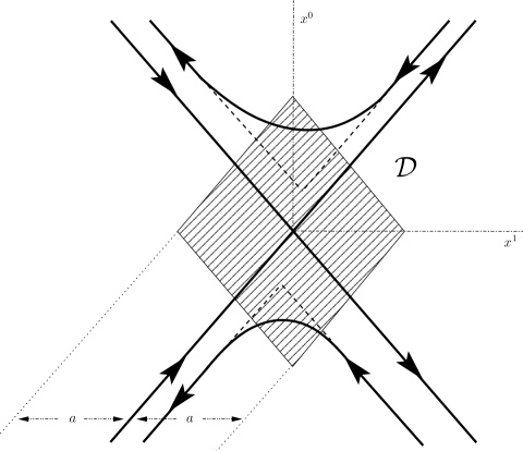
Figure 7: Spacetime region ${\cal D}$ relevant for the integration over the positions $y_{0}$ and $y_{0}^{\prime}$ of the tips of the lower and upper “wedge” in Eq. (4.42).

Taking into account that the typical paths of the exchanged fermions contributing to the path integral are expected not to depart too much from the “wedges” depicted in Fig. 4, we can thus estimate the relevant region of integration for $y_{0}$ and $y_{0}^{\prime}$ as the domain ${\cal D}$ in Fig. 7. Indeed, for $y_{0},y_{0}^{\prime}\in{\cal D}$ each of the curved Wilson lines interacts with both the straight-line ones: more precisely, in this case there is a non-negligible contribution from the interaction region near the origin of coordinates, beside the contributions at early and late times, that are cancelled by the normalisation factor and do not contribute to the scattering amplitude. This is necessary if we want that the exchanged partons be constituents of one meson, “before” the exchange, and of the other meson “after” the exchange. In the representation of the process in terms of Wilson lines, this is the counterpart of Feynman’s picture of the exchanged partons as being part of the wave functions of both the interacting hadrons.

The final step is to estimate the integral Eq. (4.42). The simplest approximation is to take $f(y_{0}^{0},y_{0}^{1},y_{0}^{\prime}{}^{0},y_{0}^{\prime}{}^{1})$ as a constant inside of ${\cal D}$ and zero outside, i.e.,

$$I_{\cal R} \simeq\int d^{2}y_{0}d^{2}y_{0}^{\prime}e^{i(p_{\bar{q}}^{\prime}+p_{q}^{\prime})\cdot y_{0}^{\prime}}e^{-i(p_{\bar{q}}+p_{q})\cdot y_{0}}f(0,0,0,0)\chi_{\cal D}(y)\chi_{\cal D}(y^{\prime})\,,$$ (4.43)

where $\chi_{\cal D}$ is the characteristic function of ${\cal D}$, which can be conveniently expressed as

$$\chi_{\cal D}(y)=\Theta\left(|y\cdot u_{1}^{\perp}|-a\cosh\frac{\chi}{2}\right)\Theta\left(|y\cdot u_{2}^{\perp}|-a\cosh\frac{\chi}{2}\right)\,,$$ (4.44)

with $\Theta(x)$ the Heaviside step function, and with $u_{i}^{\perp}$ the vector orthogonal to $u_{i}$ in Minkowski metric,

$$u_{1}^{\perp}=\left(\sinh\frac{\chi}{2},\cosh\frac{\chi}{2},\vec{0}_{\perp}\right)\,,\qquad u_{2}^{\perp}=\left(\sinh\frac{\chi}{2},-\cosh\frac{\chi}{2},\vec{0}_{\perp}\right)\,.$$ (4.45)

The integral can be easily evaluated, and for large $\chi$ it gives

$$I_{\cal R}\simeq \,f(0,0,0,0)\frac{1}{(\sinh\chi)^{2}}\left(\frac{2\pi}{m}\right)^{4}\delta_{aE}(1-\zeta_{1})\delta_{aE}(\zeta_{2})\delta_{aE}(1-\zeta_{1}^{\prime})\delta_{aE}(\zeta_{2}^{\prime})\,,$$ (4.46)

$$\delta_{\Lambda}(x) \equiv\frac{\sin\Lambda x}{\pi x}\,.$$

For large energy we recover the delta functions of Eq. (4.16), since, as it is well known, $\delta_{\Lambda}(x)\to\delta(x)$ for $\Lambda\to\infty$. However, the expression above gives us the possibility to determine how the limits $\zeta_{1}\to 1$, $\zeta_{2}\to 0$ have to be taken: since $\sin\Lambda x/x\simeq\Lambda$ when $\Lambda x\ll 1$, we have to set $\zeta_{2}\simeq 1/aE$ and $1-\zeta_{1}\simeq 1/aE$ when the energy is large. Indeed, as we will see in a moment, the integrals in the $\zeta$-variables are essentially of the form

$$I_{\alpha} =\int_{0}^{1}d\zeta\zeta^{\alpha}\frac{\sin aE\zeta}{\pi\zeta}\simeq\frac{aE}{\pi}\int_{0}^{\frac{1}{aE}}d\zeta\zeta^{\alpha}=\frac{(aE)^{-\alpha}}{\pi}\int_{0}^{1}dxx^{\alpha}$$ (4.47)

$$=\frac{(aE)^{-\alpha}}{\pi(\alpha+1)}=\frac{1}{\pi(\alpha+1)}\int_{0}^{1}d\zeta\zeta^{\alpha}\delta\left(\zeta-(aE)^{-1}\right)\,,$$

so that actually their evaluation is equivalent to setting $\zeta=1/aE$, up to numerical factors. The case of $\zeta\to 1$ is completely analogous, and the result is shown to be equivalent to setting $1-\zeta=1/aE$. In order to see how this kind of integrals comes about, we have to discuss the dependence on the $\zeta$-variables of the various quantities.

A first possible source of $\zeta$ factors are the “contracted spin factors” ${\rm S}_{\wedge}^{t_{\bar{q}}s_{q}}$ and ${\rm S}_{\vee}^{s_{q}^{\prime}t_{\bar{q}}^{\prime}}$, defined in Eq. (4.32). In order to see that they are independent of the $\zeta$-variables in a first approximation, let us write down explicitly the bispinors corresponding to $q$ and ${\bar{q}}$ (in the Dirac basis),

$$u^{(s_{q})}(p_{q}) =\sqrt{\zeta_{2}}\sqrt{E+m}\left(\begin{array}[]{c}\phi^{(s_{q})}\\ \frac{-\zeta_{2}p\sigma_{1}+\vec{p}_{q\perp}\cdot\vec{\sigma}_{\perp}}{\zeta_{2}(E+m)}\phi^{(s_{q})}\end{array}\right)\,,$$ (4.48)

$$v^{(t_{\bar{q}})}(p_{\bar{q}}) =\sqrt{1-\zeta_{1}}\sqrt{E+m}\left(\begin{array}[]{c}\frac{(1-\zeta_{1})p\sigma_{1}+\vec{p}_{{\bar{q}}\perp}\cdot\vec{\sigma}_{\perp}}{(1-\zeta_{1})(E+m)}\tilde{\phi}^{(t_{\bar{q}})}\\ \tilde{\phi}^{(t_{\bar{q}})}\end{array}\right)\,,$$

where $\phi^{(s_{q})}$ and $\tilde{\phi}^{(t_{\bar{q}})}$ are two-component spinors. The dependence on $\zeta$ is indeed of the form considered in Eq. (4.47). Moreover, since the square-root factors are canceled by the denominators of ${\rm S}_{\wedge}^{t_{\bar{q}}s_{q}}$ and ${\rm S}_{\vee}^{s_{q}^{\prime}t_{\bar{q}}^{\prime}}$, the only dependence comes from the terms involving the transverse momentum of the partons $\vec{p}_{q,{\bar{q}}\perp}=\vec{p}_{1,2\perp}/2\pm\vec{k}_{\perp}$. However, the transverse momentum $\vec{k}_{\perp}$ of a parton inside the meson is typically distributed around zero with a width approximately equal to the mass of the meson, and moreover the transverse momentum of the scattered mesons is small, due to the softness of the process. Recalling from Eq. (4.47) that $\zeta\sim 1/aE$, and that the vacuum correlation length is of the order of $a\sim 0.2\div 0.3\,{\rm fm}\sim 1\div 1.5\,{\rm GeV}^{-1}$ [64, 65, 66, 67, 68, 69], we can estimate

$$\frac{|\vec{p}_{q\perp}|}{\zeta_{2}(E+m)}\lesssim\frac{|\frac{\vec{p}_{\perp}}{2}|+|\vec{k}_{\perp}|}{\frac{1}{aE}(E+m)}\lesssim\frac{a(|\vec{q}_{\perp}|+m)}{2}\,,$$ (4.49)

which is less than one in the considered range of $t$ and for not too heavy mesons. This estimate is quite conservative, and actually we expect that the typical transverse momentum of a parton involved in the process is of the same order of $\sqrt{-t}$: for very small transferred momentum $\sqrt{-t}\ll 1\,{\rm GeV}$, we expect therefore that we can neglect the terms involving the transverse momentum of the partons, at least in a first approximation, so that the “contracted spin factors” are independent of $\zeta$.

The second source of $\zeta$-factors are the coordinate-space wave functions $\varphi_{i}(\zeta)$, where we have dropped the dependence on irrelevant variables: indeed, they contain a “kinematical” factor $\sqrt{\zeta(1-\zeta)}$, as well as any possible dependence on $\zeta$ coming from the momentum-space wave functions $\psi_{i}(\zeta)$. What matters here is the dependence on $\zeta$ near the endpoints, which we take of the usual form $\varphi_{i}(\zeta)=\zeta^{\frac{1}{2}+\beta_{i}}(1-\zeta)^{\frac{1}{2}+\gamma_{i}}g(\zeta)$ with $g(0),g(1)\neq 0$. We assume for simplicity that $\beta_{i}$, $\gamma_{i}$ are independent of the dipole size. For $\zeta\lesssim 1/(aE)\to 0$ one has that $\varphi_{i}(\zeta)\mathop{\simeq}_{\zeta\to 0}\zeta^{\frac{1}{2}+\beta_{i}}g(0)$, and in turn $\rho_{i}\mathop{\simeq}_{\zeta\to 0}\zeta^{1+2\beta_{i}}[g(0)]^{2}$ (see Eq. (4.40)), and we see therefore that the form considered in Eq. (4.47) is actually correct, with $\alpha=1+2\beta_{i}$. Similarly, for $1-\zeta\lesssim 1/(aE)\to 0$ one has that $\varphi_{i}(\zeta)\mathop{\simeq}_{\zeta\to 1}(1-\zeta)^{\frac{1}{2}+\gamma_{i}}g(1)$, and $\rho_{i}\mathop{\simeq}_{\zeta\to 1}(1-\zeta)^{1+2\gamma_{i}}[g(1)]^{2}$, and Eq. (4.47) is obtained by changing variables to $1-\zeta\to\zeta$, and setting $\alpha=1+2\gamma_{i}$.

A few comments are now in order.

• The restriction $\zeta\lesssim(aE)^{-1}$ is in accordance with Feynman’s picture of high-energy scattering [47], implying that only “wee” partons participate to the interaction. In our setting, this can be understood qualitatively in terms of uncertainty relations in the following way. Assuming that the interaction takes place in a spatial region of extension $\sim a$ in the direction of flight, one has $\Delta x\sim a$; since an exchanged parton, say, the quark $q$, belongs to the wave functions of both the interacting hadrons, its momentum can be both $+p_{q}$ and $-p_{q}$, so that $\Delta p_{x}\sim 2p_{q}\sim 2\zeta_{2}E$; finally, from $\Delta x\Delta p_{x}\sim 1$ one gets $\zeta_{2}\sim 1/2aE$.

• The approximation considered here is rather crude, and a more detailed study is needed to check if the estimate of the relevant region of integration is correct. Indeed, a different dependence of the domain ${\cal D}$ on the angle $\chi$ could change the way in which $\zeta\to 0$ as a function of energy. On the other hand, only the way in which the relevant region depends on $\chi$ is relevant to this extent, and not the detailed functional form of $f$: for example, modifying the characteristic functions $\chi_{\cal D}$ in Eq. (4.43), by substituting the Heaviside functions in Eq. (4.44) with damping exponentials, would yield again $\zeta\lesssim(aE)^{-1}$, while changing of course the numerical prefactors.

• Finally, notice that the behaviour of the wave functions near the endpoints affects the dependence on energy of the Reggeon-exchange amplitude, but only through an overall power-law factor which does not depend on $t$. In the language of Regge theory, this corresponds to a constant shift of the Regge trajectory.

This last point requires to be developed in details. We have that the Reggeon-exchange amplitude is proportional to

$${\cal A}_{{\cal R}_{1}}\propto sI_{1+2\gamma_{1}}I_{1+2\beta_{2}}\propto s(aE)^{-2(1+\gamma_{1}+\beta_{2})}=s\left(\frac{4}{a^{2}s}\right)^{1+\gamma_{1}+\beta_{2}}\sim s^{-\gamma_{1}-\beta_{2}}\,,$$ (4.50)

where $I_{\alpha}$ is defined in Eq. (4.47), and where in principle $\beta_{i},\gamma_{i}$, which appear in the meson wave function, depend on the type of meson, but not on the transferred momentum $t$. By the same token, we have for the other Reggeon-exchange amplitude

$${\cal A}_{{\cal R}_{2}}\propto sI_{1+2\gamma_{2}}I_{1+2\beta_{1}}\propto s(aE)^{-2(1+\gamma_{2}+\beta_{1})}=s\left(\frac{4}{a^{2}s}\right)^{1+\gamma_{2}+\beta_{1}}\sim s^{-\gamma_{2}-\beta_{1}}\,,$$ (4.51)

and the only thing that changes is the flavour of the exchanged fermion-antifermion pair. Notice that the right-hand side of the equations above does not contain the whole dependence on energy of the amplitude, but that nevertheless the remaining dependence is a universal function of $E/m$. Therefore, universality and degeneracy of the subleading Regge trajectories, as observed experimentally, hint to a universal behaviour of the wave functions near the endpoints. Indeed, one can immediately see that $\beta_{1}=\gamma_{2}$ and $\beta_{2}=\gamma_{1}$, by using the behaviour of the wave functions under charge conjugation, $\varphi(\vec{R},\zeta)\to\varphi^{(C)}(\vec{R},\zeta)=\eta_{c}\varphi(-\vec{R},1-\zeta)$, with $|\eta_{c}|=1$. Therefore, universality would give $\beta_{1}=\beta_{2}\equiv\beta$, and so $\varphi_{i}(\zeta)=[\zeta(1-\zeta)]^{\frac{1}{2}+\beta}g_{i}(\zeta)$, with the same $\beta$ independently of the flavours $q$ and $Q$ of the valence partons, i.e., independently of the meson. On the other hand, it would be interesting to investigate to what extent the universality of the contribution of the subleading Regge trajectory, i.e., its independence of the specific scattering process, is confirmed by experiments. We note in passing that the issue of universality of the leading contribution in the Wilson-loop formalism has been recently discussed in [22], where strong indications are found from the lattice results of [21, 14] for a universal behaviour of the relevant Wilson-loop correlation function, and therefore for the hadron-hadron total cross section.

Beside universality, another important issue is the understanding of the relation between our results and the usual picture of Regge poles in the crossed channel, which is not explicit in our formalism. A first hint is obtained through the use of gauge/gravity duality [30, 31], as we will discuss below in Section 6.

5 Analytic continuation into Euclidean space

As it is well known, path integrals are difficult to treat in Minkowski space-time outside of perturbation theory, due to the wild fluctuations of the phase factor. A more precise definition of path integrals is given by formulating them in Euclidean space, and by subsequently performing the inverse Wick rotation $x_{E4}\to ix^{0}$ to obtain a Minkowskian quantity. Moreover, a variety of techniques is available to evaluate them nonperturbatively in Euclidean space, most notably through the lattice regularisation, and, in recent times, by means of the gauge/gravity correspondence. However, physical processes happen in Minkowski space-time, and thus a Euclidean formulation can be provided only when one has established what is the Minkowskian quantity of interest. The aim of the derivation of the path-integral representation for the Reggeon-exchange amplitude, given in the previous Section, was therefore to identify such a quantity in the case of interest, and although we have not been completely rigorous from a mathematical point of view, the resulting expression should reflect the main properties of the desired amplitude.

The next step is to perform the Wick rotation of this amplitude into Euclidean space, or, more precisely, to find the Euclidean quantity whose inverse Wick rotation coincides with the given amplitude. Moreover, from the practical point of view, it is better to have a formulation of the Wick rotation of the amplitude in terms of analytic continuation relations for the “external parameters” (e.g., in the case at hand, the hyperbolic angle $\chi$ or the length parameter $T$). For this purpose, we write the dipole-dipole Reggeon-exchange amplitude in the following form:

$${\cal A}_{{\cal R}_{1}}^{(dd)}=-i2s\left(\frac{2\pi}{m}\right)^{2}\frac{1}{N_{c}}\int d^{2}b_{\perp}e^{i\vec{q}_{\perp}\cdot\vec{b}_{\perp}} (\bar{v}^{t_{\bar{q}}}(p_{\bar{q}}))_{\alpha}(u^{s_{q}}(p_{q}))_{\beta}(\bar{u}^{s_{q}^{\prime}}(p_{q}^{\prime}))_{\alpha^{\prime}}(v^{t_{\bar{q}}^{\prime}}(p_{\bar{q}}^{\prime}))_{\beta^{\prime}}$$ (5.1)

$$\times{\cal F}_{\alpha\beta;\alpha^{\prime}\beta^{\prime}}(\chi,T;\vec{b}_{\perp},\vec{R}_{1\perp},\vec{R}_{2\perp},\vec{R}_{1\perp}^{\prime},\vec{R}_{2\perp}^{\prime})\,,$$

where we have introduced the quantity

$${\cal F}_{\alpha\beta;\alpha^{\prime}\beta^{\prime}}(\chi,T;\vec{b}_{\perp},\vec{R}_{1\perp},\vec{R}_{2\perp},\vec{R}_{1\perp}^{\prime},\vec{R}_{2\perp}^{\prime})=$$ (5.2)

$$\phantom{l}\int_{2T-L_{0}}^{2T+L_{0}}dL\int_{x_{i}^{(\wedge)}}^{x_{f}^{(\wedge)}}[{\cal D}X]\int[{\cal D}\Pi]\int_{2T-L_{0}}^{2T+L_{0}}dL^{\prime}\int_{x_{i}^{(\vee)}}^{x_{f}^{(\vee)}}[{\cal D}X^{\prime}]\int[{\cal D}\Pi^{\prime}]e^{-i(m_{q}-i\epsilon)(L+L^{\prime}-4T)}$$

$$\phantom{dioladronacciacci}\times({\cal M}_{-T,-T+L}[\dot{X},\Pi])_{\alpha\beta}({\cal M}_{-T,-T+L^{\prime}}[\dot{X}^{\prime},\Pi^{\prime}])_{\alpha^{\prime}\beta^{\prime}}\,{\cal U}_{\cal C}[X,L,X^{\prime},L^{\prime}]\,.$$

As we will show below, this is the quantity which admits a convenient Euclidean representation, from which it could be obtained by means of rather simple analytic continuation relations. Since spinor indices play no role in the discussion, we will drop them in the following. Moreover, Lorentz invariance allows to restrict to the case of positive hyperbolic angle, without any loss of information [27]: in the following we will therefore take $\chi>0$.

What we expect is that the analytic continuation into Euclidean space can be achieved by performing the appropriate analytic continuation in the variables $\chi$ and $T$, as it happens in the case of the Pomeron-exchange amplitude [23, 24, 25, 26, 27, 28, 29]. To show that this is essentially the case, we follow the approach of [29], which we briefly recall. The main idea is to perform an appropriate rescaling of fields and coordinates, in order to show explicitly the dependence on these variables in the action, while removing it from the other terms. In the case of the Pomeron-exchange amplitude there is no integration over trajectories, but only the functional integration over the gluonic and fermionic fields. In that case the procedure succeeds completely, and it is possible to give a nonperturbative justification to the analytic continuation relations by inspecting the domain of convergence of the functional integral. In the case at hand, we have to deal also with the integration over the trajectories and over the momenta of the exchanged particles: as we will show below, the dependence on the relevant variables cannot be completely removed from the spin factor. As a consequence, the derivation of the analytic continuation relation that we give is formal, and its validity relies on the assumption of an appropriate analyticity domain.

We proceed now with the derivation. We define $T=\xi\tilde{T}$, and rescale the gluon fields as follows:

$$A_{\mu}(x) =\phi_{\nu}(z)M^{\nu}_{\phantom{\nu}\mu}(\chi,\xi)\,,\qquad z^{\mu}=M^{\mu}_{\phantom{\mu}\nu}(\chi,\xi)x^{\nu}$$ (5.3)

$$M^{\mu}_{\phantom{\mu}\nu}(\chi,\xi) ={\rm diag}\left(\frac{1}{\sqrt{2}\xi\cosh\frac{\chi}{2}},\frac{1}{\sqrt{2}\xi\sinh\frac{\chi}{2}},1,1\right)\,.$$

After the rescaling we obtain $\chi,\xi$-dependent expressions for the Yang-Mills action and for the fermion-matrix determinant, expressed as functionals of the new gauge field $\phi(z)$, i.e., $S_{\rm YM}[A(x)]=S_{M\chi,\xi}[\phi(z)]$, ${\cal Q}[A(x)]={\cal Q}_{M\chi,\xi}[\phi(z)]$, whose explicit forms are not relevant here, and which can be found in [29]. We make this explicit by rewriting the expectation value with respect to the rescaled fields as $\langle\ldots\rangle_{A}=\langle\ldots\rangle_{{M\chi,\xi}}$. Moreover, we define $L_{0}=\xi\tilde{L}_{0}$, and we rescale the integration variables in the path integrals as follows,

$$Z^{\mu}=M^{\mu}_{\phantom{\mu}\nu}(\chi,\xi)X^{\nu}\,,\qquad\Pi_{\mu}=\rho_{\nu}M^{\nu}_{\phantom{\nu}\mu}(\chi,\xi)\,,\qquad L=\xi\tilde{L}\,,$$ (5.4)

and similarly for primed quantities. After these transformations, we obtain for ${\cal F}$ the expression

$${\cal F} (\chi,T;\vec{b}_{\perp},\vec{R}_{1\perp},\vec{R}_{2\perp},\vec{R}_{1\perp}^{\prime},\vec{R}_{2\perp}^{\prime})=\tilde{\cal F}(\chi,\xi;\tilde{T};\vec{b}_{\perp},\vec{R}_{1\perp},\vec{R}_{2\perp},\vec{R}_{1\perp}^{\prime},\vec{R}_{2\perp}^{\prime})\equiv$$ (5.5)

$$\left(\frac{1}{\xi\sinh\chi}\right)^{2}\int_{2\tilde{T}-\tilde{L}_{0}}^{2\tilde{T}+\tilde{L}_{0}}d\tilde{L}\int_{z_{i}^{(\wedge)}}^{z_{f}^{(\wedge)}}[{\cal D}Z]\int[{\cal D}\rho]\int_{2\tilde{T}-\tilde{L}_{0}}^{2\tilde{T}+\tilde{L}_{0}}d\tilde{L}^{\prime}\int_{z_{i}^{(\vee)}}^{z_{f}^{(\vee)}}[{\cal D}Z^{\prime}]\int[{\cal D}\rho^{\prime}]$$

$$\phantom{diosp}\times e^{-im_{q}\xi(\tilde{L}+\tilde{L}^{\prime}-4\tilde{T})}\tilde{{\cal M}}_{-\tilde{T},-\tilde{T}+\tilde{L}}[\dot{Z},\rho]\tilde{{\cal M}}_{-\tilde{T},-\tilde{T}+\tilde{L}^{\prime}}[\dot{Z}^{\prime},\rho^{\prime}]\tilde{\cal U}_{\tilde{\cal C}}[\chi,\xi;Z,\tilde{L},Z^{\prime},\tilde{L}^{\prime}]\,,$$

where we have denoted the spin factors expressed in terms of the new variables as

$$\tilde{{\cal M}}_{-\tilde{T},-\tilde{T}+\tilde{L}}[\dot{Z},\rho]={\rm Texp} \left[i\int_{-\tilde{T}}^{-\tilde{T}+\tilde{L}}d\tau\left(\xi\rho_{\mu}(\tau)M^{\mu}_{\phantom{\mu}\nu}(\chi,\xi)\gamma^{\nu}-\rho_{\mu}(\tau)\dot{Z}^{\mu}(\tau)\right)\right]\,,$$ (5.6)

and similarly for $\tilde{{\cal M}}_{-\tilde{T},-\tilde{T}+\tilde{L}^{\prime}}[\dot{Z}^{\prime},\rho^{\prime}]$, and where the normalised expectation value $\tilde{\cal U}_{\tilde{\cal C}}$,

$$\tilde{\cal U}_{\tilde{\cal C}}[\chi,\xi;Z,\tilde{L},Z^{\prime},\tilde{L}^{\prime}]={\langle\tilde{{\cal W}}_{\tilde{\cal C}}[Z,\tilde{L},Z^{\prime},\tilde{L}^{\prime}]\rangle_{{M\chi,\xi}}}\Big{[}\langle\tilde{{\cal W}}_{1}^{\tilde{T}}(\vec{b}_{\perp},\vec{R}_{1\perp})\rangle_{{M\chi,\xi}}\langle\tilde{{\cal W}}_{2}^{\tilde{T}}(\vec{0}_{\perp},\vec{R}_{2\perp})\rangle_{{M\chi,\xi}}\\ \times\langle\tilde{{\cal W}}_{1}^{\tilde{T}}(\vec{b}_{\perp}-\Delta\vec{R}_{1\perp},\vec{R}_{1\perp}^{\prime})\rangle_{{M\chi,\xi}}\langle\tilde{{\cal W}}_{2}^{\tilde{T}}(\Delta\vec{R}_{2\perp},\vec{R}_{2\perp}^{\prime})\rangle_{{M\chi,\xi}}\Big{]}^{-1}\,,$$ (5.7)

is defined in terms of the Wilson loops

$$\tilde{{\cal W}}_{\tilde{\cal C}}[Z,\tilde{L},Z^{\prime},\tilde{L}^{\prime}] =\frac{1}{N_{c}}\,{\rm tr}\,{\rm Texp}\left\{-ig\oint_{\tilde{\cal C}}\phi_{\mu}(z)dz^{\mu}\right\}\,,$$ (5.8)

$$\tilde{{\cal W}}_{i}^{\tilde{T}}(\vec{d}_{i\perp},\vec{D}_{i\perp}) =\frac{1}{N_{c}}\,{\rm tr}\,{\rm Texp}\left\{-ig\oint_{\tilde{\bar{{\cal C}}}^{(i)}(\vec{d}_{\perp},\vec{D}_{\perp})}\phi_{\mu}(z)dz^{\mu}\right\}\,.$$

The paths entering Eq. (5.8) are defined as follows,

$$\tilde{\cal C}=\tilde{\cal C}^{(1)}_{+}\circ\tilde{\cal C}^{(\vee)}\circ\tilde{\cal C}^{(2)}_{-}\circ\tilde{\cal C}^{(\wedge)}\,,\quad\tilde{\bar{{\cal C}}}^{(i)}(\vec{d}_{\perp},\vec{D}_{\perp})=\tilde{\bar{{\cal C}}}^{(i)}_{+}(\vec{d}_{\perp},\vec{D}_{\perp})\circ\tilde{\bar{{\cal C}}}^{(i)}_{-}(\vec{d}_{\perp},\vec{D}_{\perp})\,,\quad i=1,2\,,$$ (5.9)

and the various pieces are given by the following expressions: for the straight-line parts,

$$\tilde{\cal C}^{(1)}_{+}:\,\,Z^{(1)}_{+}(\tau)=n_{1}\tau+b+\frac{R_{1}}{2}\,,\qquad\tilde{\cal C}^{(2)}_{-}:\,\,Z^{(2)}_{-}(\tau)=-n_{2}\tau-\frac{R_{2}}{2}\,,$$ (5.10)

with $\tau\in[-\tilde{T},\tilde{T}]$, and

$$\tilde{\bar{{\cal C}}}^{(i)}_{\pm}(\vec{d}_{\perp},\vec{D}_{\perp}):\,\,\tilde{\bar{Z}}^{(i)}_{\pm}(\tau)=\pm n_{i}\tau+d\pm\frac{D}{2}\,,$$ (5.11)

with $\tau\in[-\frac{\tilde{T}}{2},\frac{\tilde{T}}{2}]$, where

$$n_{1}=\frac{1}{\sqrt{2}}(1,1,\vec{0}_{\perp})\,,\quad n_{2}=\frac{1}{\sqrt{2}}(1,-1,\vec{0}_{\perp})\,,\quad d=(0,0,\vec{d}_{\perp})\,,\quad D=(0,0,\vec{D}_{\perp})\,,$$ (5.12)

while for the curved parts

$$\tilde{\cal C}^{(\wedge)}: ~{}Z(\tau),\qquad\phantom{{}^{\prime}}\tau\in[-\tilde{T},-\tilde{T}+\tilde{L}]\,,$$ (5.13)

$$~{}Z(-\tilde{T})=-n_{2}\tilde{T}+\frac{R_{2}}{2}=z_{i}^{(\wedge)}\,, Z(-\tilde{T}+\tilde{L})=-n_{1}\tilde{T}+b-\frac{R_{1}}{2}=z_{f}^{(\wedge)}\,,$$

$$\tilde{\cal C}^{(\vee)}: ~{}Z^{\prime}(\tau),\qquad\tau\in[-\tilde{T},-\tilde{T}+\tilde{L}^{\prime}]\,,$$

$$~{}Z^{\prime}(-\tilde{T})=n_{1}\tilde{T}+b-R_{1}^{\prime}+\frac{R_{1}}{2}=z_{i}^{(\vee)}\,, Z^{\prime}(-\tilde{T}+\tilde{L}^{\prime})=n_{2}\tilde{T}+R_{2}^{\prime}-\frac{R_{2}}{2}=z_{f}^{(\vee)}\,.$$

The various pieces are connected by the appropriate straight-line paths in the transverse plane at $\tau=\pm\tilde{T}$ or $\tau=\pm\tilde{T}/2$, which we are not writing down explicitly. As we have already mentioned, the only dependence left on $\chi$ and $\xi$ is in the rescaled action, and in the $\gamma$-matrix term in the spin factor. Also, additional dependence could appear when introducing the appropriate regularisation, which is required to make the spin factor a mathematically meaningful quantity [45, 46]. For the time being we are therefore unable to give a complete proof for the analytic continuation, including the determination of a sufficiently wide analyticity domain. Here we limit ourselves to the determination of the appropriate relation which allows to go from Minkowski to Euclidean space, and viceversa, assuming the existence of such a domain.

The stage is now set to determine the form of the analytic continuation into Euclidean space. We know from [29] that performing the analytic continuation $\xi\to-i\eta,\chi\to i\theta$, the Yang-Mills action and the fermion-matrix determinant go over into rescaled versions of the Euclidean Yang-Mills action and of the Euclidean fermion-matrix determinant, respectively. More precisely, the rescaled Euclidean action $S_{E{\rm YM}}[A_{E}(x_{E})]=S_{E\theta,\eta}[\phi(z)]$, and the rescaled Euclidean fermion-matrix determinant ${\cal Q}_{E}[A_{E}(x_{E})]={\cal Q}_{E\theta,\eta}[\phi(z)]$, are obtained by performing the following transformation of fields and coordinates,

$$z^{\mu} =M_{E\mu\nu}P_{\nu\rho}x_{E\rho}\,,\qquad A_{E\mu}(x_{E})=\phi_{\rho}(z)P_{\rho\nu}M_{E\nu\mu}$$ (5.14)

$$M_{E\mu\nu} ={\rm diag}\left(\frac{1}{\sqrt{2}\eta\cos\frac{\theta}{2}},\frac{1}{\sqrt{2}\eta\sin\frac{\theta}{2}},1,1\right)\,,$$

where the matrix $P$ permutes the components of the Euclidean coordinates in order to put them in the order $4123$, and the values 0 and 4 of the spacetime index are identified. The use of a contravariant index for the Euclidean coordinate causes no ambiguity. The relation between the Minkowskian and Euclidean action and fermion-matrix determinant is expressed as

$$S_{E\theta,\eta}[\phi(z)]=S_{Mi\theta,-i\eta}[\phi(z)]\,,\qquad{\cal Q}_{E\theta,\eta}[\phi(z)]={\cal Q}_{Mi\theta,-i\eta}[\phi(z)]\,.$$ (5.15)

The analytic continuation Eq. (5.15) is valid for $\theta\in(0,\pi)$, and starting from the analytic expression at $\chi>0$ in Minkowski space. The restriction on $\theta$ does not cause any loss of information, due to the $O(4)$ invariance of the Euclidean theory [27]. Performing now the analytic continuation $\xi\to-i\eta,\chi\to i\theta$ in (5.5), we obtain

$$\tilde{\cal F} (i\theta,-i\eta;\tilde{T};\vec{b}_{\perp},\vec{R}_{1\perp},\vec{R}_{2\perp},\vec{R}_{1\perp}^{\prime},\vec{R}_{2\perp}^{\prime})=\tilde{\cal F}_{E}(\theta,\eta;\tilde{T};\vec{b}_{\perp},\vec{R}_{1\perp},\vec{R}_{2\perp},\vec{R}_{1\perp}^{\prime},\vec{R}_{2\perp}^{\prime})\equiv$$ (5.16)

$$\left(\frac{1}{\eta\sin\theta}\right)^{2}\int_{2\tilde{T}-\tilde{L}_{0}}^{2\tilde{T}+\tilde{L}_{0}}d\tilde{L}\int_{z_{i}^{(\wedge)}}^{z_{f}^{(\wedge)}}[{\cal D}Z]\int[{\cal D}\rho]\int_{2\tilde{T}-\tilde{L}_{0}}^{2\tilde{T}+\tilde{L}_{0}}d\tilde{L}^{\prime}\int_{z_{i}^{(\vee)}}^{z_{f}^{(\vee)}}[{\cal D}Z^{\prime}]\int[{\cal D}\rho^{\prime}]$$

$$\phantom{trem}\times e^{-m_{q}\eta(\tilde{L}+\tilde{L}^{\prime}-4\tilde{T})}\tilde{{\cal M}}^{(E)}_{-\tilde{T},-\tilde{T}+\tilde{L}}[\dot{Z},\rho]\tilde{{\cal M}}^{(E)}_{-\tilde{T},-\tilde{T}+\tilde{L}^{\prime}}[\dot{Z}^{\prime},\rho^{\prime}]\tilde{\cal U}^{(E)}_{\tilde{\cal C}}[\theta,\eta;Z,\tilde{L},Z^{\prime},\tilde{L}^{\prime}]\,,$$

where we have used the notation

$$\tilde{{\cal M}}^{(E)}_{-\tilde{T},-\tilde{T}+\tilde{L}}[\dot{Z},\rho] ={\rm Texp}\left[i\int_{-\tilde{T}}^{-\tilde{T}+\tilde{L}}d\tau\left(\eta\rho_{\mu}(\tau)M_{E\mu\nu}(\theta,\eta)\gamma_{E\nu}-\rho_{\mu}(\tau)\dot{Z}^{\mu}(\tau)\right)\right]\,,$$ (5.17)

and similarly for $\tilde{{\cal M}}^{(E)}_{-\tilde{T},-\tilde{T}+\tilde{L}^{\prime}}[\dot{Z}^{\prime},\rho^{\prime}]$, for the analytically-continued spin factor, with $\gamma_{E\mu}$ the Euclidean gamma-matrices $\gamma_{E0}=\gamma^{0}$, $\gamma_{Ej}=-i\gamma^{j}$, and

$$\tilde{\cal U}^{(E)}_{\tilde{\cal C}}[\theta,\eta;Z,\tilde{L},Z^{\prime},\tilde{L}^{\prime}]=\langle\tilde{{\cal W}}_{\tilde{\cal C}}[Z,\tilde{L},Z^{\prime},\tilde{L}^{\prime}]\rangle_{{E\theta,\eta}}\Big{[}\langle\tilde{{\cal W}}_{1}^{\tilde{T}}(\vec{b}_{\perp},\vec{R}_{1\perp})\rangle_{{E\theta,\eta}}\langle\tilde{{\cal W}}_{2}^{\tilde{T}}(\vec{0}_{\perp},\vec{R}_{2\perp})\rangle_{{E\theta,\eta}}\\ \times\langle\tilde{{\cal W}}_{1}^{\tilde{T}}(\vec{b}_{\perp}-\Delta\vec{R}_{1\perp},\vec{R}_{1\perp}^{\prime})\rangle_{{E\theta,\eta}}\langle\tilde{{\cal W}}_{2}^{\tilde{T}}(\Delta\vec{R}_{2\perp},\vec{R}_{2\perp}^{\prime})\rangle_{{E\theta,\eta}}\Big{]}^{-1}\,,$$ (5.18)

for the analytically-continued normalised expectation value. Notice that the Wilson loops in Eq. (5.18) are exactly the same defined above in Eq. (5.8). The expectation value obtained using the rescaled Euclidean Yang-Mills action and rescaled Euclidean fermion-matrix determinant has been denoted with $\langle\ldots\rangle_{E\theta,\eta}$.

Now, we already know from [29] that the expectation values $\langle\tilde{{\cal W}}_{i}^{\tilde{T}}\rangle_{{E\theta,\eta}}$ in Eq. (5.18) are simply the expression in terms of the rescaled Euclidean action of the expectation values $\langle{\cal W}^{(E)\,T_{E}}_{i}\rangle_{E}$, where $\langle\ldots\rangle_{E}$ is the expectation value in the sense of the usual Euclidean functional integral, and the Wilson loops ${\cal W}^{(E)\,T_{E}}_{i}$ are defined as follows,

$${\cal W}^{(E)\,T_{E}}_{i}(\vec{d}_{\perp},\vec{D}_{\perp})=\frac{1}{N_{c}}\,{\rm tr}\,{\rm Texp}\left\{-ig\oint_{\bar{{\cal C}}_{E}^{(i)}(\vec{d}_{\perp},\vec{D}_{\perp})}A_{E}(x_{E})\cdot dx_{E}\right\}\,,$$ (5.19)

where the dot stands for the Euclidean scalar product, and the paths are defined as

$$\bar{{\cal C}}_{E}^{(i)}(\vec{d}_{\perp},\vec{D}_{\perp})=\bar{{\cal C}}^{(i)}_{E+}(\vec{d}_{\perp},\vec{D}_{\perp})\circ\bar{{\cal C}}^{(i)}_{E-}(\vec{d}_{\perp},\vec{D}_{\perp})\,,\quad i=1,2\,,$$ (5.20)

with the various pieces being given by the straight lines

$$\bar{{\cal C}}^{(i)}_{E\pm}(\vec{d}_{\perp},\vec{D}_{\perp}) :\,\bar{X}^{(i)}_{E\pm}(\tau)=\pm u_{Ei}\tau+d_{E}\pm\frac{D_{E}}{2}\,,$$ (5.21)

with $\tau\in[-\textstyle\frac{{T}_{E}}{2},\textstyle\frac{{T}_{E}}{2}]$, having set $T_{E}=\eta\tilde{T}$, and with

$$u_{E1} =(\sin\theta,\vec{0}_{\perp},\cos\theta)\,, u_{E2} =(-\sin\theta,\vec{0}_{\perp},\cos\theta)\,,$$ (5.22)

$$d_{E} =(0,\vec{d}_{\perp},0)\,, D_{E} =(0,\vec{D}_{\perp},0)\,,$$

and moreover closed by appropriate straight-line paths in the transverse plane at $\pm T_{E}/2$. In particular, $d_{E}$ and $D_{E}$ take the following values, $d_{E}=0$, $b_{E}$, $b_{E}-\Delta R_{E1}$, $\Delta R_{E2}$ and $D_{E}=R_{E1,2}$, $R_{E1,2}^{\prime}$, with

$$b_{E}=(0,\vec{b}_{\perp},0)\,,\quad R_{Ei}=(0,\vec{R}_{i\perp},0)\,,\quad R_{Ei}^{\prime}=(0,\vec{R}_{i\perp}^{\prime},0)\,,\quad\Delta R_{Ei}=(0,\Delta\vec{R}_{i\perp},0)\,.$$ (5.23)

To see what the other terms correspond to in the Euclidean theory expressed through the usual variables, we have to rescale back coordinates and momenta in the path integral according to the following transformations,

$$Z^{\mu}=M_{E\mu\nu}P_{\nu\rho}X_{E\nu}\,,\qquad\Pi_{E\mu}=\rho_{\rho}P_{\rho\nu}M_{E\nu\mu}\,,$$ (5.24)

and moreover to set ${L}_{E0}=\eta\tilde{L}_{0}$, ${L}_{E}=\eta\tilde{L}$, and similarly for primed quantities. It is then immediate to see that the analytically-continued spin factor is simply the rescaled version of the usual Euclidean spin factor,

$${{\cal M}}^{(E)}_{-T_{E},T_{E}+L_{E}}[\dot{X}_{E},\Pi_{E}] ={\rm Texp}\left[i\int_{-T_{E}}^{T_{E}+{L}_{E}}d\tau\left({\raisebox{0.8pt}{\makebox[0.0pt][l]{\bf{ /}}}{\Pi}}_{E}(\tau)-\Pi_{E}(\tau)\cdot\dot{X}_{E}(\tau)\right)\right]\,,$$ (5.25)

with ${\raisebox{0.8pt}{\makebox[0.0pt][l]{\bf{ /}}}{\Pi}}_{E}=\Pi_{E\mu}\gamma_{E\mu}$, and similarly for ${{\cal M}}^{(E)}_{-T_{E},T_{E}+L^{\prime}_{E}}[\dot{X}^{\prime}_{E},\Pi_{E}^{\prime}]$; also, the expectation value $\langle\tilde{{\cal W}}_{\tilde{\cal C}}[Z,\tilde{L},Z^{\prime},\tilde{L}^{\prime}]\rangle_{{E\theta,\eta}}$ is equal to the usual expectation value $\langle{\cal W}^{(E)}_{{\cal C}_{E}}[X_{E},{L}_{E},X_{E}^{\prime},{L}_{E}^{\prime}]\rangle_{E}$ of the following Euclidean Wilson loop,

$${\cal W}^{(E)}_{{\cal C}_{E}}[X_{E},{L}_{E},X_{E}^{\prime},{L}_{E}^{\prime}]= \frac{1}{N_{c}}\,{\rm tr}\,{\rm Texp}\left\{-ig\oint_{{\cal C}_{E}}A_{E}(x_{E})\cdot dx_{E}\right\}\,,$$ (5.26)

where the path ${\cal C}_{E}$ is defined as

$${\cal C}_{E} ={\cal C}^{(1)}_{E+}\circ{\cal C}_{E}^{(\vee)}\circ{\cal C}^{(2)}_{E-}\circ{\cal C}_{E}^{(\wedge)}\,,$$ (5.27)

with ${\cal C}^{(1)}_{E+}$, ${\cal C}^{(2)}_{E-}$ given by

$${\cal C}^{(1)}_{E+} :\,X^{(1)}_{E+}(\tau)=u_{E1}\tau+b_{E}+\frac{R_{E1}}{2}\,, {\cal C}^{(2)}_{E-} :\,X^{(2)}_{E-}(\tau)=-u_{E2}\tau-\frac{R_{E2}}{2}\,,$$ (5.28)

with $\tau\in[-{T}_{E},{T}_{E}]$, and moreover

$${\cal C}_{E}^{(\wedge)}: ~{}X_{E}(\tau)\,,\qquad\phantom{{}^{\prime}}\tau\in[-{T}_{E},-{T}_{E}+{L}_{E}]$$ (5.29)

$$~{}X_{E}(-{T}_{E})=-u_{E2}{T}_{E}+\frac{R_{E2}}{2} X_{E}(-{T}_{E}+{L}_{E})=-u_{E1}{T}_{E}+b_{E}-\frac{R_{E1}}{2}$$

$$~{}\phantom{X_{E}(-{T}_{E})}=x_{Ei}^{(\wedge)}\,, \phantom{X_{E}(-{T}_{E}+{L}_{E})}=x_{Ef}^{(\wedge)}\,,$$

$${\cal C}_{E}^{(\vee)}: ~{}X^{\prime}_{E}(\tau)\,,\qquad\tau\in[-{T}_{E},-{T}_{E}+{L}_{E}^{\prime}]$$

$$~{}X^{\prime}_{E}(-{T}_{E})=u_{E1}{T}_{E}+b_{E}-R_{E1}^{\prime}+\frac{R_{E1}}{2} X^{\prime}_{E}(-{T}_{E}+{L}_{E}^{\prime})=u_{E2}{T}_{E}+R_{E2}^{\prime}-\frac{R_{E2}}{2}\,,$$

$$~{}\phantom{X^{\prime}_{E}(-{T}_{E})}=x_{Ei}^{(\vee)}\,, \phantom{X^{\prime}_{E}(-{T}_{E}+{L}_{E}^{\prime})}=x_{Ef}^{(\vee)}\,.$$

It turns out therefore that $\tilde{\cal F}_{E}$ is simply the rescaled version of ${\cal F}_{E}$,

$$\tilde{\cal F}_{E}(\theta,\eta;\tilde{T};\vec{b}_{\perp},\vec{R}_{1\perp},\vec{R}_{2\perp},\vec{R}_{1\perp}^{\prime},\vec{R}_{2\perp}^{\prime})={\cal F}_{E}(\theta,T_{E};\vec{b}_{\perp},\vec{R}_{1\perp},\vec{R}_{2\perp},\vec{R}_{1\perp}^{\prime},\vec{R}_{2\perp}^{\prime})\,,$$ (5.30)

where

$${\cal F}_{E}(\theta,T_{E};\vec{b}_{\perp},\vec{R}_{1\perp},\vec{R}_{2\perp},\vec{R}_{1\perp}^{\prime},\vec{R}_{2\perp}^{\prime})=$$ (5.31)

$$\int_{2T_{E}-L_{E0}}^{2T_{E}+L_{E0}}d{L}_{E}\int_{x_{Ei}^{(\wedge)}}^{x_{Ef}^{(\wedge)}}[{\cal D}X_{E}]\int[{\cal D}\Pi_{E}]\int_{2T_{E}-L_{E0}}^{2T_{E}+L_{E0}}d{L}_{E}^{\prime}\int_{x_{Ei}^{(\vee)}}^{x_{Ef}^{(\vee)}}[{\cal D}X_{E}^{\prime}]\int[{\cal D}\Pi_{E}^{\prime}]$$

$$\phantom{madiaaa}\times e^{-m_{q}({L}_{E}+{L}_{E}^{\prime}-4T_{E})}{{\cal M}}^{(E)}_{-T_{E},-T_{E}+L_{E}}[\dot{X}_{E},\Pi_{E}]{{\cal M}}^{(E)}_{-T_{E},T_{E}+L_{E}^{\prime}}[\dot{X}_{E}^{\prime},\Pi_{E}^{\prime}]\,$$

$$\phantom{madiaaa}\times{\cal U}^{(E)}_{{\cal C}_{E}}[X_{E},L_{E},X_{E}^{\prime},L_{E}^{\prime}]\,,$$

where the Euclidean normalised expectation value is given by

$${\cal U}^{(E)}_{{\cal C}_{E}}[X_{E},L_{E},X_{E}^{\prime},L_{E}^{\prime}]\equiv\langle{\cal W}^{(E)}_{\cal C}[X_{E},L_{E},X_{E}^{\prime},L_{E}^{\prime}]\rangle_{E}\Big{[}\langle{\cal W}^{(E)\,T_{E}}_{1}(\vec{b}_{\perp},\vec{R}_{1\perp})\rangle_{E}\\ \times\langle{\cal W}^{(E)\,T_{E}}_{2}(\vec{0}_{\perp},\vec{R}_{2\perp})\rangle_{E}\langle{\cal W}^{(E)\,T_{E}}_{1}(\vec{b}_{\perp}-\Delta\vec{R}_{1\perp},\vec{R}_{1\perp}^{\prime})\rangle_{E}\langle{\cal W}^{(E)\,T_{E}}_{2}(\Delta\vec{R}_{2\perp},\vec{R}_{2\perp}^{\prime})\rangle_{E}\Big{]}^{-1}\,.$$ (5.32)

In conclusion, comparing Eqs. (5.5), (5.16) and (5.30), we obtain the desired analytic continuation relations connecting the Minkowskian quantity ${\cal F}$, entering the expression for the Reggeon-exchange amplitude, and its Euclidean counterpart ${\cal F}_{E}$,

$${\cal F}_{E}(\theta,T_{E},L_{E0};\vec{b}_{\perp},\vec{R}_{1\perp},\vec{R}_{2\perp},\vec{R}_{1\perp}^{\prime},\vec{R}_{2\perp}^{\prime}) ={\cal F}(i\theta,-iT_{E},-iL_{E0};\vec{b}_{\perp},\vec{R}_{1\perp},\vec{R}_{2\perp},\vec{R}_{1\perp}^{\prime},\vec{R}_{2\perp}^{\prime})\,,$$ (5.33)

$${\cal F}(\chi,T,L_{0};\vec{b}_{\perp},\vec{R}_{1\perp},\vec{R}_{2\perp},\vec{R}_{1\perp}^{\prime},\vec{R}_{2\perp}^{\prime}) ={\cal F}_{E}(-i\chi,iT,iL_{0};\vec{b}_{\perp},\vec{R}_{1\perp},\vec{R}_{2\perp},\vec{R}_{1\perp}^{\prime},\vec{R}_{2\perp}^{\prime})\,.$$

The relations Eq. (5.33), which allow to reconstruct the physical Reggeon-exchange amplitude from a calculation in Euclidean space, call for a few remarks.

• The analytic continuation relations Eq. (5.33) are similar to those obtained in the case of the Pomeron-exchange amplitude, the only modification being that we also have to perform $L_{E0}\to iL_{0}$. This can be a non trivial task, since it requires the determination of the precise analytic dependence on $L_{E0}$. However, if the Euclidean path integral saturates at a certain characteristic value of $L_{E}$, at which all the relevant contributions have been included, it would be possible to take $L_{E0}\to\infty$ without changing appreciably the result.

• The dependence on $T_{E}$ is expected to become trivial in the limit $T_{E}\to\infty$, the argument being the same given in the Minkowskian case. If ${\cal F}$, ${\cal F}_{E}$ have finite limits as $T,T_{E}\to\infty$, as we expect, and moreover if they satisfy appropriate analyticity assumptions, it is possible to prove that in the limit $T,T_{E}\to\infty$ the analytic continuation relations simplify, reducing to the analytic continuation $\theta\to-i\chi$, $L_{E0}\to iL_{0}$ only. The argument is based on the Phragmén-Lindelöf theorem, and can be easily adapted from Ref. [26]. The same argument can be applied to the dependence on $L_{E0}$: if we can take the limits $L_{E0}\to\infty$ and $L_{0}\to\infty$ without changing appreciably the results, with the appropriate analyticity assumptions it is possible to prove in the same way that in this limit the analytic continuation reduces simply to $\theta\to-i\chi$.

• As we have already said, at the present stage we are not in the position to determine the domain of analyticity of ${\cal F}$ and ${\cal F}_{E}$, and thus the domain of validity of Eq. (5.33). Consider ${\cal F}_{E}$ for definiteness. In order to make these relations meaningful, it is necessary that the analyticity domain ${\cal D}_{E}$ of ${\cal F}_{E}$ contains the real segment $(0,\pi)$ at ${\rm Re\,}{\eta}>0,{\rm Im\,}{\eta}=0$, and the negative imaginary half-axis $i\theta\in(0,\infty)$ at ${\rm Re\,}{\eta}=0,{\rm Im\,}{\eta}>0$.  This has been tacitly assumed when deriving the analytic continuation relations Eq. (5.33). Under this hypothesis, the analytic continuation relations would therefore allow to reconstruct the physical Minkowskian amplitude at $\chi>0$ starting from the Euclidean quantity ${\cal F}_{E}$ in the interval $\theta\in(0,\pi)$.

• The main obstacle in carrying over here the discussion of Ref. [29] is the dependence on $\theta,\eta$ (resp. $\chi,\xi$) of the rescaled Euclidean (resp. Minkowskian) spin factor. Since the integrand is an analytic function of the relevant variables, the criterion for analyticity is the convergence of the functional integral over gauge fields, and of the path integrals over the trajectories $X,X^{\prime}$ and the momenta $\Pi,\Pi^{\prime}$. It is known [42, 43, 45, 46] that, as it stands, the integral over momenta is not converging even in Euclidean space, and that an appropriate regularisation is needed. Multiplying the integrand by a factor $e^{-\int_{\nu_{i}}^{\nu_{f}}d\nu\,\epsilon(\nu)\sqrt{\Pi_{E}(\nu)^{2}}}$ [72], it can be shown that [45, 46]

  $${\cal S}_{\nu_{i},\nu_{f}}^{(E)}[\dot{X}_{E}]\equiv\int[{\cal D}\Pi_{E}]\,{{\cal M}}^{(E)}_{\nu_{i},\nu_{f}}[\dot{X}_{E},\Pi_{E}]=\prod_{\nu=\nu_{i}}^{\nu_{f}}\delta\left(1-\big{(}\dot{X}_{E}(\nu)\big{)}^{2}\right)\frac{1+{\raisebox{0.65pt}{\makebox[0.0pt][l]{\bf{ /}}}{\dot{X}_{E}}}(\nu)}{2}\,,$$ (5.34)

  when the regularisation is removed, i.e., $\epsilon(\nu)\to 0$. A detailed study of the analyticity domain of ${\cal F}$ should therefore start from the study of convergence of the integration over momenta of the regularised spin factor, for complex values of the variables $\theta,\eta$. This requires further work, which is outside the scope of the present paper.

The expression Eq. (5.31), together with the analytic continuation relations Eq. (5.33), provide the basis for the Euclidean approach to the Reggeon-exchange amplitude suggested in Ref. [30]. In the next Section we make contact with the proposal of [30], and with the more recent investigations on the same line discussed in [31].

6 Reggeon exchange and gauge/gravity duality

In this Section we want to make contact with the previous analysis of the Reggeon-exchange amplitude in a Euclidean setting [30, 31]. In particular, we want to discuss how the basic expression proposed there for the Reggeon-exchange amplitude is related to the one obtained in this paper. We will refer in particular to the more recent and more detailed analysis contained in Ref. [31].

The process considered in Ref. [31] is the elastic scattering of two heavy-light mesons $M_{1,2}$ of large mass $m_{1,2}$, i.e., $M_{1}=Q{\bar{q}}$ and $M_{2}={\bar{Q}}^{\prime}q$, where $Q$ and ${\bar{Q}}^{\prime}$ are heavy and of different flavours, while $q$ and ${\bar{q}}$ are light and of the same flavour. This choice was made in order to have a single type of Reggeon exchange, namely the one in which the interacting mesons exchange the valence $q$ and ${\bar{q}}$ partons. Moreover, the choice of heavy mesons is made so that the typical sizes of the constituent dipoles are small, $|\vec{R}_{i\perp}|\sim m_{i}^{-1}\ll\Lambda_{\rm QCD}^{-1}$. In this way, in a first approximation one can focus directly on the dipole-dipole Reggeon-exchange amplitude, ignoring the integration over the dipole size and orientation.

It is straightforward to adapt the calculations of the previous Sections to this case. First of all, the relation between $\chi$ and $s$ at high energy is modified to $\chi\simeq\log(s/m_{1}m_{2})$; moreover, Eq. (2.17) simplifies to

$$S_{fi}^{(dd)}={\cal P}^{(dd)}+{\cal R}_{1}^{(dd)}\,.$$ (6.1)

The rest of the derivation is not modified, in particular the expressions Eqs. (4.39) and (4.41) for the Reggeon-exchange amplitude and the analytic continuation relations Eq. (5.33) remain unchanged.

Introducing now the following shorthand notation for the normalised Wilson-loop expectation value and for the spin factor,

$${\cal U}^{(E)}[{\cal C}_{E}] ={\cal U}^{(E)}_{{\cal C}_{E}}[X_{E},L_{E},X_{E}^{\prime},X_{E}^{\prime}]\,,$$ (6.2)

$${\cal I}[{\cal C}_{E}] ={{\cal S}}^{(E)}_{-T_{E},-T_{E}+L_{E}}[\dot{X}_{E}]{{\cal S}}^{(E)}_{-T_{E},T_{E}+L_{E}^{\prime}}[\dot{X}_{E}^{\prime}]\,,$$

where ${{\cal S}}^{(E)}_{\nu_{i},\nu_{f}}$ has been defined in Eq. (5.34), and moreover denoting the path integrals as follows,

$$\int{\cal DC}_{E}^{(\wedge)} =\int_{2T_{E}-L_{E0}}^{2T_{E}+L_{E0}}d{L}_{E}\int[{\cal D}X_{E}]\,,$$ (6.3)

$$\int{\cal DC}_{E}^{(\vee)} =\int_{2T_{E}-L_{E0}}^{2T_{E}+L_{E0}}d{L}_{E}^{\prime}\int[{\cal D}X_{E}^{\prime}]\,,$$

we can write

$${\cal F}_{E}(\theta,T_{E};\vec{b}_{\perp},\vec{R}_{1\perp},\vec{R}_{2\perp},\vec{R}_{1\perp}^{\prime},\vec{R}_{2\perp}^{\prime})=\\ \int{\cal DC}_{E}^{(\vee)}\int{\cal DC}_{E}^{(\wedge)}\,e^{-m_{q}({L}_{E}+{L}_{E}^{\prime}-4T_{E})}{\cal U}^{(E)}[{\cal C}_{E}]{\cal I}[{\cal C}_{E}]\,.$$ (6.4)

One can now easily be convinced by a simple comparison that ${\cal F}_{E}$ is the same quantity as the “Euclidean amplitude” $\tilde{a}$ of Eq. (3.3) in Ref. [31].

It is then possible, at this point, to carry out the analysis performed in that paper. Here we will not repeat the analysis in details, but simply summarise the main points. The basic idea is to employ the gauge/gravity duality in a confining background in order to evaluate the Wilson loop expectation values entering Eq. (6.4). The first precise formulation of this duality, the well known AdS/CFT correspondence [73, 74, 75], relates the weak-coupling, supergravity limit of type IIB string theory in $AdS_{5}\times S^{5}$, to four-dimensional ${\cal N}=4$ SYM theory, which is a conformal (and thus non confining) field theory, in the limit of large number of colours $N_{c}$ and strong ’t Hooft coupling $\lambda=g_{\rm YM}^{2}N_{c}$. In particular, the AdS/CFT correspondence gives the following area-law prescription for the expectation value of a Wilson loop running along the path ${\cal C}_{E}$ in Euclidean space [34, 35, 36, 37],

$$\langle{\cal W}[{\cal C}_{E}]\rangle={\cal F}l[{\cal C}_{E}]e^{-\frac{1}{2\pi\alpha^{\prime}}A_{\rm min}[{\cal C}_{E}]}\,.$$ (6.5)

Here $A_{\rm min}$ is the area of the minimal surface in the Euclidean version of the $AdS_{5}$ metric (i.e., in hyperbolic space), $1/(2\pi\alpha^{\prime})=\sqrt{\lambda}/(2\pi)$ is the string tension, and ${\cal F}l[{\cal C}_{E}]$ stands for the contribution of quantum fluctuations around the minimal surface.

Although various attempts have been made, a precise formulation of the duality for QCD is not known yet (assuming it exists). Nevertheless, a few general properties of the gravity dual of a confining theory have been established: in particular, the presence of a confinement scale in the gauge theory translates into a characteristic scale $R_{0}$ in the metric of the gravity theory, associated for example to the horizon of a black hole [76], or to the position of a hard wall [77], or to the scale associated to a soft wall [78]. Such a scale essentially separates the regions of small and large $z$, where $z$ is the fifth coordinate of AdS space: while for small $z$ the metric diverges as some inverse power of $z$, for $z$ of the order of $R_{0}$ the metric turns out to be effectively flat. Moreover, the area-law prescription Eq. (6.5) carries over to the confining case, substituting the AdS metric with an appropriate confining background [38, 39, 40] and replacing $1/(2\pi\alpha^{\prime})$ with an effective string tension $1/(2\pi\alpha^{\prime}_{\rm eff})$.

At this point, one has to substitute the area-law expression Eq. (6.5), with the minimal surface determined in the appropriate confining metric, into the path integral Eq. (6.4). The resulting expression is still too difficult to deal with, not to mention the fact that the exact metric to be used is not yet known. In order to obtain an estimate, a few approximations are therefore needed.

The general features of the metric described above suggest a convenient approximation scheme to evaluate the Wilson-loop expectation value in a generic confining background [18]. The small-$z$ behaviour suggests that, in order to minimise the area, it is convenient for the surface to rise almost vertically from the boundary, without appreciable motion in the other directions, at least when the typical size of the Wilson loop is not too small. The presence of a horizon puts an upper bound on this vertical rise; moreover, when $z\sim R_{0}$, the surface lives effectively in flat space. As a result, the minimal surface is expected to be constituted by two parts: an almost vertical wall rising from the boundary up to the horizon, and transporting there the boundary conditions, and a solution of the Plateau problem in flat space.

The solution of the Plateau problem in the general case is not known even in flat space. Nevertheless, the particular configuration in the case at hand suggests that the relevant contributions to the path integral come from those trajectories of the exchanged fermions which lie on the helicoid determined by the eikonal trajectories of the “spectator” fermions [30, 31]. In particular, the small dipole size makes the dependence on the dipole orientation trivial in a first approximation. This leads to the following approximation for the path integral Eq. (6.4),

$${\cal F}_{E}(\theta,T_{E};\vec{b}_{\perp},\vec{R}_{1\perp},\vec{R}_{2\perp},\vec{R}_{1\perp}^{\prime},\vec{R}_{2\perp}^{\prime})\approx\int{\cal DC}_{E}^{(\vee)}\int{\cal DC}_{E}^{(\wedge)}\,e^{-S_{\rm eff}[{\cal C}_{E}^{(\vee)},\,{\cal C}_{E}^{(\wedge)}]}{\cal I}[{\cal C}_{E}]\,,$$ (6.6)

where the “effective action” $S_{\rm eff}$ is given by

$$S_{\rm eff}=\frac{1}{2\pi\alpha^{\prime}_{\rm eff}}A_{\rm min}[{\cal C}_{E}^{(\vee)},\,{\cal C}_{E}^{(\wedge)}]+\hat{m}_{q}\big{(}L_{E}[{\cal C}_{E}^{(\vee)}]+L_{E}[{\cal C}_{E}^{(\wedge)}]-4T_{E}\big{)}\,,$$ (6.7)

and the Euclidean paths of the exchanged fermions ${\cal C}_{E}^{(\vee)}$, ${\cal C}_{E}^{(\wedge)}$ are constrained to lie on the helicoid determined by the paths ${\cal C}_{E+}^{(1)}$ and ${\cal C}_{E-}^{(2)}$. Here $L[{\cal C}_{E}^{(\vee),(\wedge)}]$ denote the length of the Euclidean paths of the exchanged fermions. Ultraviolet divergencies require a renormalisation of the quark mass to $\hat{m}_{q}$ [31].

The final step is a saddle-point approximation of Eq. (6.6). The saddle point is determined by minimising the functional Eq. (6.7). The detailed calculations are reported in [30], for the massless quark case $\hat{m}_{q}=0$, and in [31] for the more general case of a massive quark, and will not be discussed here. We simply mention that an exact solution to the saddle-point equations can be found in implicit form for $b\leq b_{c}=4\pi\alpha^{\prime}_{\rm eff}\hat{m}_{q}$, with $b=|\vec{b}_{\perp}|$ the impact-parameter distance. An explicit solution can be obtained in the case of small angles $\theta$, and we report here the corresponding result for the “effective action” Eq. (6.7):

$$S_{\rm eff}=\frac{b^{2}}{2\pi\alpha_{\rm eff}^{\prime}\theta}{\rm arccosh}\frac{b_{c}}{b}+2\pi^{2}\alpha_{\rm eff}^{\prime}\hat{m}_{q}^{2}-\frac{2b\hat{m}_{q}}{\theta}\sqrt{\left(\frac{b_{c}}{b}\right)^{2}-1}\,.$$ (6.8)

At this point one has to perform the analytic continuation to Minkowski space. Although the expression Eq. (6.8) is valid only at small $\theta$, it is nevertheless worth to investigate what it leads to. Notice that there is no dependence on $T_{E}$, as expected. After analytic continuation, the resulting expression can be extended to $b>b_{c}$, as it is explained in [31], so that it is possible to take the limit of small quark mass. Up to order ${\cal O}(\alpha_{\rm eff}^{\prime}\hat{m}_{q}^{2})$,

$$S_{{\rm eff},\,M}\simeq\frac{b^{2}}{4\alpha_{\rm eff}^{\prime}\chi}-\frac{4b\hat{m}_{q}}{\chi}+2\pi^{2}\alpha_{\rm eff}^{\prime}\hat{m}_{q}^{2}\,,$$ (6.9)

where we have denoted with $S_{{\rm eff},\,M}$ the analytic continuation of $S_{{\rm eff}}$ to Minkowski spacetime. Rewriting now the dipole-dipole Reggeon-exchange scattering amplitude Eq. (4.41) in the impact-parameter representation,

$${\cal A}_{{\cal R}_{1}}^{(dd)}(s,t)=-i2s\int d^{2}b_{\perp}e^{i\vec{q}_{\perp}\cdot\vec{b}_{\perp}}a_{{\cal R}_{1}}^{(dd)}(\chi,\vec{b}_{\perp})$$ (6.10)

where we have dropped the dependence on the dipole sizes and the spin indices, and substituting the result Eq. (6.9) in it, one finds (to first order in $\sqrt{\alpha_{\rm eff}^{\prime}}\hat{m}_{q}$)

$$a_{{\cal R}_{1}}^{(dd)}(\chi,\vec{b})\approx e^{-\frac{b^{2}}{4\alpha_{\rm eff}^{\prime}\chi}}\left(1+\frac{4b\hat{m}_{q}}{\chi}\right)\times{\cal K}\,.$$ (6.11)

Here we have put in ${\cal K}$ all the remaining factors, including the contribution of the spin factor, those of the quantum fluctuations ${\cal F}l[{\cal C}_{E}]$ (see Eq. (6.5)) of the string around the minimal surface, and the determinant coming from the integration of quadratic fluctuations of the boundary around the saddle-point. As discussed in [31], this expression leads to a linear Reggeon trajectory $\alpha(t)=\alpha_{0}+\alpha_{\rm eff}^{\prime}t$, although the Regge singularity is not simply a pole when $\hat{m}_{q}\neq 0$, but contains also a logarithmic branch point. This result is independent of possible prefactors $s^{\delta\alpha}\chi^{n_{\chi}}b^{n_{b}}$ (with $n_{\chi},n_{b}\in\mathbb{N}$), which could be present in ${\cal K}$, but which are not under control at the present stage. In particular, a factor $s^{\delta\alpha}$ simply shifts the trajectory by a constant amount, while $\chi^{n_{\chi}}b^{n_{b}}$ can change the order of the pole but neither the Regge trajectory nor the presence of a logarithmic branch point [31].

Some important remarks are in order.

• The extra factor of $s$ in Eqs. (4.41) and (6.10) is removed by the integration over the longitudinal momentum fraction, as can be seen from Eqs. (4.50) and (4.51). More precisely, the overall power of $s$ at $t=0$, i.e., the “Reggeon intercept” $\alpha_{0}$, depends on the end-point behaviour of the mesonic wave functions, as discussed at the end of Section 4. The simplest choice, corresponding to the phenomenological Wirbel-Stech-Bauer ansatz [60] where the dependence on $\zeta_{1}$ and $\zeta_{2}$ is purely “kinematical” (i.e., $\alpha_{1,2}=\beta_{1,2}=0$ in Eqs. (4.50) and (4.51); cfr. also Eq. (2.10)), gives an intercept $\alpha_{0}=0$.

• The spin factor ${\cal I}[{\cal C}_{E}]$ (see Eq. (6.2)) has been evaluated in exact but implicit form in [31], but the corresponding small-$\theta$ approximation has been shown not to lead to a fully reliable analytic continuation into Minkowski space-time. A more detailed study is needed in order to clarify its possible effects. We mention however that, independently of the small-$\theta$ approximation, it contains a factor which behaves as $s^{-1}$, after analytic continuation to Minkowski space-time: this factor cancels the (four) factors $\sqrt{E+m}$ appearing in Eq. (4.48), when contracting with the Dirac bispinors.

• The quantity ${\cal F}l[{\cal C}_{E}]$ has been evaluated in [30] in the massless-quark case, where it leads to a factor $s^{\frac{n_{\perp}}{24}}$, with $n_{\perp}$ the number of transverse directions in which the string can fluctuate, which increases the Reggeon intercept. The corresponding calculation in the case of massive quarks is more difficult, due to the nontrivial form of the resulting minimal surface, and it has not been performed yet.

• The evaluation of the effect of fluctuations of the boundary around the saddle point solution requires first of all a precise formulation of the saddle-point approximation for the path-integral Eq. (6.4), which is not available at the moment.

• The fact that the Regge slope is equal to the inverse of the string tension, which appears in the confining potential, is a first indication in order to understand the relation between our formalism based on Wilson loops and the usual picture of Regge poles. Indeed, in this picture the Regge trajectory $\alpha(t)$ at $t>0$ provides the relation between the mass $M$ and the spin $J$ of the “families” of particles exchanged in the scattering process, i.e., $J=\alpha(M^{2})=\alpha_{0}+\alpha_{1}M^{2}$; in turn, in the QCD-string picture the slope $\alpha_{1}$ is exactly the inverse of the string tension. Combining these results, one is led to expect that the same $\alpha_{1}$ appears in the Regge trajectory and in the static potential, an expectation that is met by the above result, with $\alpha_{1}=\alpha_{\rm eff}^{\prime}$.

The investigation of these issues is beyond the scope of this paper, and more work is needed in order to complete the dual gravity picture of soft high-energy scattering.

7 Conclusions and Outlook

In this paper we have proposed a derivation of a nonperturbative expression for the scattering amplitude of the Reggeon-exchange process in high-energy elastic meson-meson scattering. Using a partonic description of hadrons, along the lines of [2], such a process is identified with the exchange between the mesons of a (Reggeised) pair of valence fermions, as in Refs. [30, 31]. Exploiting a path-integral representation of the various fermionic propagators, and retaining only the paths which are expected to give relevant contributions at high energy, we have been able to express the Reggeon-exchange amplitude in terms of a path-integral of the (properly normalised) expectation value of a certain Wilson loop, over the trajectories of the exchanged fermions. The relevant trajectories are determined by the constraint that they coincide with the eikonal trajectories far away from the interaction region. Moreover, under certain analyticity assumptions, we have shown how the Reggeon-exchange amplitude can be reconstructed from a Euclidean quantity by means of an appropriate analytic continuation, which is very similar to the one [26, 27, 28, 29] employed in the case of the leading, Pomeron-exchange amplitude. We have also shown that the expression derived in this paper is essentially the same one proposed in [30] and recently reconsidered in [31], and we have briefly discussed how a saddle-point approximation can be qualitatively performed in Euclidean space, making use of gauge/gravity duality for a confining background and restricting the trajectories of the exchanged fermions to a special class, namely trajectories lying on the helicoid determined by the “spectator” partons’ trajectories. The results obtained in this approximation are in qualitative agreement with the phenomenology.

Let us now briefly summarise the main open issues of the approach discussed in this paper.

• In the course of the derivation of the Reggeon-exchange amplitude we have made a few technical assumptions on the path-integral representation of the propagators, which need to be investigated in detail. In particular, the identification of the nature of the parameter along the path requires a detailed study of the integration over momenta in the path integral in Minkowski space, which would yield an explicit expression for the Minkowskian spin factor.

• According to our results, the dependence on energy of the Reggeon-exchange amplitude is affected by the behaviour of the mesonic wave functions near the value $0$ for the longitudinal momentum fractions of the fermions which are exchanged in the process. In order to reconcile this result with the experimentally observed universality of the subleading contributions to total cross sections, we are led to assume that such a behaviour is a universal feature of the nonperturbative wave functions describing the mesons in terms of colourless dipoles. On the other hand, it would be interesting to understand to what extent the universality of the subleading contribution is established experimentally.

• A study of the analyticity domain of the relevant quantities is necessary, in order to properly justify the analytic continuation relations. The features of this analyticity domain are expected to be related with the convergence properties of the path integral for complex values of the relevant variables, similarly to what has been discussed in Ref. [29] in the Pomeron-exchange case.

• As regards the gauge/gravity duality approach employed in Refs. [30, 31], further work is needed in order to obtain a precise formulation of the saddle-point approximation of the relevant path integral. Such a formulation would allow to write down the saddle-point equation for the whole range of paths, and not only for the class of paths which gives a predetermined, helicoidal geometry for the Euclidean minimal surface. It would also clarify how the fluctuations of the trajectories around the saddle-point solution discussed in Refs. [30, 31] have to be properly taken into account.

In conclusion, we hope that further work in these directions could help in a better understanding of soft high-energy scattering, and the related issue of a first-principle explanation of Regge phenomenology.

Appendix A Eikonal approximation for straight-line trajectories

In this Appendix we rederive the eikonal approximation Eq. (3.2) for the truncated-connected propagator of a fermion in an external field, using the path-integral formalism.

Using the trick described in [57], appropriately generalised to the case of fermions, the truncated-connected propagator for a quark $Q$ of “physical” mass $\tilde{m}_{Q}$ can be written in the path-integral representation as

$$Z_{Q}\hat{S}_{Q}={\rm Lim}\frac{1}{\nu_{f}-\nu_{i}}\bar{u}(p_{Q}^{\prime})\left(\tilde{F}(\nu_{f},\nu_{i})-\tilde{F}(\nu_{f},\nu_{f})\right)u(p_{Q})\,,$$ (A.1)

where

$$\tilde{F}(\nu_{f},\nu_{i}) =\int[{\cal D}X]\int[{\cal D}\Pi]\,e^{i[p_{Q}^{\prime}\cdot X(\nu_{f})-p_{Q}\cdot X(\nu_{i})]}e^{-i(\nu_{f}-\nu_{i})(m-i\epsilon)}$$ (A.2)

$$\phantom{\int[{\cal D}X]\int[{\cal D}\Pi]\,}\times{\cal M}_{\nu_{i},\nu_{f}}[X,\Pi]{W}_{\nu_{i},\nu_{f}}[X]\,,$$

$$\tilde{F}(0,0) =\int d^{4}x\,e^{i(p_{Q}^{\prime}-p_{Q})\cdot x}\,,$$

bispinors are normalised as in Eq. (2.20), and we recall that

$${\cal M}_{\eta,\nu}[X,\Pi] ={\rm Texp}\left[i\int_{\eta}^{\nu}d\tau\left({\raisebox{0.8pt}{\makebox[0.0pt][l]{\bf{ /}}}{\Pi}}(\tau)-\Pi(\tau)\cdot\dot{X}(\tau)\right)\right]\,,$$ (A.3)

$${W}_{\eta,\nu}[X] ={\rm Texp}\left[-ig\int_{\eta}^{\nu}d\tau A(X(\tau))\cdot\dot{X}(\tau)\right]\,.$$

Assuming the dominance of the classical trajectory of the quark,

$$X(\tau)=\frac{p_{Q}}{\tilde{m}_{Q}}(\tau-\nu_{i})+X(\nu_{i})\,,$$ (A.4)

where $p_{Q}$ has been defined in Eq. (2.5), the path integral for $\tilde{F}(\nu_{f},\nu_{i})$ reduces to an integration over the initial point $x_{i}\equiv X(\nu_{i})$, the final point being determined by the relation $x_{f}\equiv X(\nu_{f})=\frac{p_{Q}}{\tilde{m}_{Q}}(\nu_{f}-\nu_{i})+x_{i}$. In the description of mesons in terms of colourless $q{\bar{q}}$ dipoles, the “physical” quark mass $\tilde{m}_{Q}$ is identified with the fraction of meson mass carried by the quark in the initial state, $\tilde{m}_{Q}=\zeta m$, which in principle can be different from the fraction $\tilde{m}_{Q}^{\prime}=\zeta^{\prime}m$ carried in the final state. However, we have seen that for soft high-energy scattering one finds $\zeta=\zeta^{\prime}$, when the eikonal propagator is inserted in the expressions for the scattering amplitude. Here we proceed by keeping them distinct: this does not affect the trajectory, since $\frac{p_{Q}}{\tilde{m}_{Q}}=\frac{p}{m}=u$ and $\frac{p_{Q}^{\prime}}{\tilde{m}_{Q}^{\prime}}=\frac{p^{\prime}}{m}=u$, where $p\simeq p^{\prime}$ and $m$ are the initial and final momentum and the mass of the meson. As for the integration over $\Pi$, the saddle point is given by $\Pi(\tau)=p_{Q}$, since in that case, given the fact that we are “sandwiching” between bispinors, ${\raisebox{0.8pt}{\makebox[0.0pt][l]{\bf{ /}}}{\Pi}}(\tau)-\Pi(\tau)\cdot\dot{X}(\tau)={\raisebox{-0.5pt}{\makebox[0.0pt][l]{\bf{ /}}}{p}}_{Q}-\tilde{m}_{Q}\to 0$; choosing $\Pi(\tau)=p_{Q}^{\prime}$ yields the same result. The integration along the direction parallel to $u$ is trivial, since in the limit of infinite length we have translational invariance along $u$. In practice, writing $x_{i,f}=b+\nu_{i,f}u$, so that $b=(\nu_{f}x_{i}-\nu_{i}x_{f})/(\nu_{f}-\nu_{i})$, we have

$$p_{Q}^{\prime}\cdot x_{f}-p_{Q}\cdot x_{i}=(p^{\prime}-p)\cdot b+(\tilde{m}_{Q}^{\prime}\nu_{f}-\tilde{m}_{Q}\nu_{i})\,,$$ (A.5)

and thus, replacing the spin factor with unity, we find that

$$\tilde{F}(\nu_{f},\nu_{i})\simeq \int d^{4}x_{i}\,e^{i(p_{Q}^{\prime}\cdot x_{f}-p_{Q}\cdot x_{i})}e^{-i(\nu_{f}-\nu_{i})(m_{Q}-i\epsilon)}\,{W}_{\nu_{f},\nu_{i}}\left[\textstyle\frac{p_{Q}}{\tilde{m}_{Q}}(\tau-\nu_{i})+x_{i}\right]=$$ (A.6)

$$e^{i[(\tilde{m}_{Q}^{\prime}-m_{Q})\nu_{f}-(\tilde{m}_{Q}-m_{Q})\nu_{i}]}\int d^{4}b\,e^{i(p^{\prime}-p)\cdot b}\,W_{u}(b)=$$

$$e^{i[(\tilde{m}_{Q}^{\prime}-m_{Q})\nu_{f}-(\tilde{m}_{Q}-m_{Q})\nu_{i}]}\int_{\nu_{i}}^{\nu_{f}}d\nu\int d^{3}b\,e^{-i(\vec{p}^{\,\prime}-\vec{p})\cdot\vec{b}}\,W_{u}(b)=$$

$$(\nu_{f}-\nu_{i})e^{i[(\tilde{m}_{Q}^{\prime}-m_{Q})\nu_{f}-(\tilde{m}_{Q}-m_{Q})\nu_{i}]}\int d^{3}b\,e^{i(p^{\prime}-p)\cdot b}\,W_{u}(b)\,,$$

where through a Lorentz transformation we have set $b^{0}$ to be the coordinate parallel to $u$ and $\vec{b}$ the spatial coordinates in the rest frame of the particle, and we have used the notation $W_{u}(b)$ for a straight-line Wilson line parallel to $u$ and centered at $b$ (the value of $b^{0}$ is of course arbitrary in the limit of infinite length). As for the disconnected term, we have in the $b$-coordinates

$$\tilde{F}(0,0) =\int d^{4}be^{i(p_{Q}^{\prime}-p_{Q})\cdot b}=\int_{\nu_{i}}^{\nu_{f}}d\nu e^{i(p_{Q}^{\prime 0}-p_{Q}^{0})\nu}\int d^{3}be^{-i(\vec{p}_{Q}^{\,\prime}-\vec{p}_{Q})\cdot\vec{b}}$$ (A.7)

$$=(\nu_{f}-\nu_{i})(2\pi)^{3}\delta^{(3)}(\vec{p}_{Q\,{\rm r.f.}}^{\,\prime}-\vec{p}_{Q\,{\rm r.f.}}){\cal K}(\nu_{i},\nu_{f};\tilde{m}_{Q},\tilde{m}_{Q}^{\prime})\,,$$

where the subscript “r.f.” stands for “rest frame”, and where

$${\cal K}(\nu_{i},\nu_{f};\tilde{m}_{Q},\tilde{m}_{Q}^{\prime}) =e^{i\frac{\tilde{m}_{Q}^{\prime}-\tilde{m}_{Q}}{2}(\nu_{f}+\nu_{i})}\frac{\sin\left(\frac{\tilde{m}_{Q}^{\prime}-\tilde{m}_{Q}}{2}(\nu_{f}-\nu_{i})\right)}{\frac{\tilde{m}_{Q}^{\prime}-\tilde{m}_{Q}}{2}(\nu_{f}-\nu_{i})}\,,$$ (A.8)

$${\cal K}(\nu_{i},\nu_{f};\tilde{m}_{Q},\tilde{m}_{Q}^{\prime}) =1\,,\quad{\rm if}\,\,\tilde{m}_{Q}^{\prime}=\tilde{m}_{Q}\,,$$

$$\lim_{\nu_{f}\to\infty,\,\nu_{i}\to-\infty}{\cal K}(\nu_{i},\nu_{f};\tilde{m}_{Q},\tilde{m}_{Q}^{\prime}) =0\,,\quad{\rm if}\,\,\tilde{m}_{Q}^{\prime}\neq\tilde{m}_{Q}\,.$$

Plugging the results above in Eq. (A.1) we finally obtain

$$Z_{Q}\hat{S}_{Q} =\delta_{s_{Q}^{\prime}s_{Q}}\,2\sqrt{\tilde{m}_{Q}\tilde{m}_{Q}^{\prime}}\Big{[}e^{i[(\tilde{m}_{Q}^{\prime}-m_{Q})\nu_{f}-(\tilde{m}_{Q}-m_{Q})\nu_{i}]}\int d^{3}be^{i(p^{\prime}-p)\cdot b}W_{u}(b)$$ (A.9)

$$\phantom{2\sqrt{\tilde{m}_{Q}\tilde{m}_{Q}^{\prime}}\Big{[}e^{i[(\tilde{m}_{Q}^{\prime}-m_{Q})\nu_{f}-(\tilde{m}_{Q}-m_{Q})\nu_{i}]}}-(2\pi)^{3}\delta^{(3)}(\vec{p}_{\rm r.f.}^{\,\prime}-\vec{p}_{\rm r.f.})\Delta(\tilde{m}_{Q}^{\prime}-\tilde{m}_{Q})\Big{]}$$

$$=\delta_{s_{Q}^{\prime}s_{Q}}\,2\sqrt{\tilde{m}_{Q}\tilde{m}_{Q}^{\prime}}e^{i((\tilde{m}_{Q}^{\prime}-m_{Q})\nu_{f}-(\tilde{m}_{Q}-m_{Q})\nu_{i})}\int d^{3}be^{i(p^{\prime}-p)\cdot b}W_{u}(b)-\delta_{Q}\,,$$

where the function $\Delta(x)$ is defined as $\Delta(x)=1$ if $x=0$, and 0 otherwise. In the last passage we have recognised that the disconnected term is the expression in the rest frame of the invariant delta-function Eq. (2.6), in which we have included also $\Delta(\tilde{m}_{Q}^{\prime}-\tilde{m}_{Q})$, which is essentially a superselection rule on the particle species. The prefactor comes from the contraction of the Dirac bispinors, which in the high-energy limit gives ($\vec{p}_{Q}\parallel x^{1}$)

$$\bar{u}^{s_{Q}^{\prime}}(p_{Q}^{\prime})u^{s_{Q}}(p_{Q}) =\delta_{s_{Q}^{\prime}s_{Q}}\,\sqrt{(E_{Q}^{\prime}+\tilde{m}_{Q}^{\prime})(E_{Q}+\tilde{m}_{Q})}\left(1-\frac{|\vec{p}_{Q}^{\,\prime}||\vec{p}_{Q}|}{(E_{Q}^{\prime}+\tilde{m}_{Q}^{\prime})(E_{Q}+\tilde{m}_{Q})}\right)$$ (A.10)

$$=\delta_{s_{Q}^{\prime}s_{Q}}\,2m\sqrt{\zeta\zeta^{\prime}}=\delta_{s_{Q}^{\prime}s_{Q}}\,2\sqrt{\tilde{m}_{Q}\tilde{m}_{Q}^{\prime}}\,.$$

The expression for the eikonal propagator is only apparently different from the one already known in the literature (up to the phase factor). Indeed, if we replace the integration over $b^{1}$, which is the coordinate in the longitudinal plane orthogonal to $u_{1}$, with the integration over the longitudinal coordinate parallel to $u_{2}$, and rescale it so that it becomes a light-cone coordinate in the high-energy limit $\chi\to\infty$, we recover the well-known result [2, 57, 7]. Explicitly, setting $q=p^{\prime}-p$, we have

$$(q\cdot u_{1}^{\perp})b^{1} =\left[q\cdot\left(\coth\chi u_{1}-\frac{1}{\sinh\chi}u_{2}\right)\right]b^{1}=-(q\cdot u_{2})\frac{b^{1}}{\sinh\chi}$$ (A.11)

$$=-q\cdot\frac{u_{2}}{\cosh\frac{\chi}{2}}\frac{b^{1}}{2\sinh\frac{\chi}{2}}\,.$$

We introduce now lightcone coordinates as follows, $b=(b_{+}u_{+}+b_{-}u_{-})/2+b_{\perp}$, where $b_{\pm}=b^{0}\pm b^{1}$ and $b_{\perp}=(0,0,\vec{b}_{\perp})$, and the lightcone vectors are defined as $u_{\pm}=(1,\pm 1,\vec{0}_{\perp})$. The Minkowskian scalar product is rewritten as $q\cdot b=(q_{+}b_{-}+q_{-}b_{+})/2+q_{\perp}\cdot b_{\perp}$. Since in the large-$\chi$ limit $\frac{u_{2}}{\cosh\frac{\chi}{2}}\to u_{-}$ , and moreover $q_{-}\simeq 0$, we have that $b_{-}=-\frac{b^{1}}{\sinh\frac{\chi}{2}}$, and thus for $\chi\to\infty$ we have

$$Z_{Q}\hat{S}_{Q}+\delta_{Q}=2\sqrt{\zeta\zeta^{\prime}}Ee^{i(\tilde{m}_{Q}^{\prime}+\tilde{m}_{Q}-2m_{Q})T}\int[d^{3}b]\,e^{iq\cdot b}\,{W}_{u_{+}}(b)\,,$$ (A.12)

where now ${W}_{u_{+}}(b)$ is a Wilson line running along the $+$ lightcone direction, $[d^{3}b]$ includes trasverse coordinates and the $-$ lightcone coordinate, and we have set $\nu_{f}=-\nu_{i}=T$ for simplicity.

References

[1] P. D. B. Collins, An Introduction to Regge Theory
and High-Energy Physics, (Cambridge University Press, Cambridge,
1977).
[2] O. Nachtmann, Ann. Phys. 209 (1991) 436.
[3] H. Lehmann, K. Symanzik, and W. Zimmermann, Nuovo
Cim. 1 (1955) 205.
[4] H. Lehmann, K. Symanzik, and W. Zimmermann, Nuovo
Cim. 6 (1957) 319.
[5] H. G. Dosch, E. Ferreira and A. Krämer,
Phys. Rev. D 50 (1994) 1992 [arXiv:hep-ph/9405237].
[6] O. Nachtmann, in Perturbative and
nonperturbative aspects of quantum field theory,
edited by H. Latal and W. Schweiger
(Springer-Verlag, Berlin, Heidelberg, 1997), 49; in Lectures on
QCD: Applications, edited by H. W. Grießhammer, F. Lenz and
D. Stoll (Springer-Verlag, Berlin, Heidelberg, 1997), 1
[arXiv:hep-ph/9609365].
[7] E. Meggiolaro, Phys. Rev. D 53 (1996)
3835 [arXiv:hep-th/9506043].
[8] E. R. Berger and O. Nachtmann, Eur. Phys. J. C 7
(1999) 459 [arXiv:hep-ph/9808320].
[9] E. Meggiolaro, Nucl. Phys. B 602 (2001)
261 [arXiv:hep-ph/0009261].
[10]
H.G. Dosch, in At the frontier of Particle Physics – Handbook of QCD
(Boris Ioffe Festschrift), edited by M. Shifman (World Scientific, Singapore,
2001), vol. 2, 1195.
[11] A. I. Shoshi, F. D. Steffen and H. J. Pirner,
Nucl. Phys. A 709 (2002) 131 [arXiv:hep-ph/0202012].
[12] A. I. Shoshi, F. D. Steffen, H. G. Dosch and
H. J. Pirner, Phys. Rev. D 68 (2003) 074004
[arXiv:hep-ph/0211287].
[13] E. Shuryak and I. Zahed, Phys. Rev. D 62
(2000) 085014 [arXiv:hep-ph/0005152].
[14] M. Giordano and E. Meggiolaro, Phys. Rev. D
81 (2010) 074022 [arXiv:0910.4505 [hep-ph]].
[15]
R. A. Janik and R. Peschanski, Nucl. Phys. B 565 (2000) 193
[arXiv:hep-th/9907177].
[16] M. Giordano
and R. Peschanski, JHEP 1005 (2010) 037 [arXiv:1003.2309
[hep-ph]].
[17] M. Giordano, R. Peschanski, and S. Seki,
Acta Phys. Polon. B 43 (2012) 1289 [arXiv:1110.3680 [hep-th]].
[18]
R. A. Janik and R. B. Peschanski, Nucl. Phys. B 586 (2000)
163 [arXiv:hep-th/0003059].
[19]
R. A. Janik, Phys. Lett. B 500 (2001) 118 [arXiv:hep-th/0010069].
[20] G. Başar, D. E. Kharzeev, H. -U. Yee and I. Zahed,
Phys. Rev. D 85 (2012) 105005 [arXiv:1202.0831 [hep-th]].
[21]
M. Giordano and E. Meggiolaro,
Phys. Rev. D 78 (2008) 074510 [arXiv:0808.1022
[hep-lat]].
[22] M. Giordano, E. Meggiolaro and N. Moretti,
arXiv:1203.0961 [hep-ph].
[23] E. Meggiolaro, Z. Phys. C 76 (1997)
523 [arXiv:hep-th/9602104].
[24] E. Meggiolaro, Eur. Phys. J. C 4 (1998)
101 [arXiv:hep-th/9702186].
[25] E. Meggiolaro, Nucl. Phys. B 625 (2002)
312 [arXiv:hep-ph/0110069].
[26] E. Meggiolaro, Nucl. Phys. B 707
(2005) 199 [arXiv:hep-ph/0407084].
[27]
M. Giordano and E. Meggiolaro, Phys. Rev. D 74 (2006)
016003 [arXiv:hep-ph/0602143].
[28]
E. Meggiolaro, Phys. Lett. B 651 (2007) 177
[arXiv:hep-ph/0612307].
[29] M. Giordano and E. Meggiolaro, Phys. Lett. B
675 (2009) 123 [arXiv:0902.4145 [hep-ph]].
[30] R. A. Janik and R. B. Peschanski,
Nucl. Phys. B 625 (2002) 279 [arXiv:hep-th/0110024].
[31] M. Giordano and R. Peschanski,
JHEP 1110 (2011) 108 [arXiv:1105.6013 [hep-th]].
[32] E. Avsar, Y. Hatta, and T. Matsuo, JHEP 1003
(2010) 037 [arXiv:0912.3806 [hep-th]].
[33] Y. Makeenko, Phys. Rev. D 83 (2011) 026007
[arXiv:1012.0708 [hep-th]].
[34] J. Maldacena, Phys. Rev. Lett. 80 (1998)
4859. [arXiv:hep-th/9803002].
[35] S. -J. Rey and J. Yee, Eur. Phys. Jour. C 22 (2001) 379 [arXiv:hep-th/9803001].
[36] D. J. Gross and H. Ooguri, Phys. Rev. D 58 (1998)
106002 [arXiv:hep-th/9805129].
[37] N. Drukker, D. J. Gross and H. Ooguri,
Phys. Rev. D 60 (1999) 125006
[arXiv:hep-th/9904191].
[38] A. Brandhuber, N. Itzhaki, J. Sonnenschein and
S. Yankielowicz, JHEP 9806 (1998) 001
[arXiv:hep-th/9803263].
[39] Y. Kinar, E. Schreiber and J. Sonnenschein,
Nucl. Phys. B 566 (2000) 103
[arXiv:hep-th/9811192].
[40] Y. Kinar, E. Schreiber, J. Sonnenschein and N. Weiss,
Nucl. Phys. B 583 (2000) 76
[arXiv:hep-th/9911123].
[41] E. S. Fradkin, Proc. Int. Winter School on
Theoretical Physics at JINR (Dubna, 1964); Acta Phys. Hung. XIX (1965) 175.
[42] R. A. Brandt, F. Neri, and D. Zwanziger,
Phys. Rev. D 19 (1979) 1153.
[43] R. A. Brandt, A. Gocksch,
M. Sato, and F. Neri, Phys. Rev. D 26 (1982) 3611.
[44] A. M. Polyakov, Mod. Phys. Lett. A 3
(1988) 325.
[45] G. P. Korchemsky, Phys. Lett. B232 (1989)
334.
[46] G. P. Korchemsky, Int. J. Mod. Phys. A 7
(1992) 339.
[47] R. P. Feynman, Phys. Rev. Lett. 23 (1969) 1415.
[48]
H. Verlinde and E. Verlinde, arXiv:hep-th/9302104.
[49]
A. H. Mueller, Nucl. Phys. B 415 (1994) 373.
[50]
A. H. Mueller, Nucl. Phys. B 437 (1995) 107
[arXiv:hep-ph/9408245].
[51]
A. H. Mueller and B. Patel, Nucl. Phys. B 425 (1994) 471
[arXiv:hep-ph/9403256].
[52]
C. Ewerz and O. Nachtmann, Annals Phys. 322 (2007) 1635
[arXiv:hep-ph/0404254].
[53]
C. Ewerz and O. Nachtmann, Annals Phys. 322 (2007) 1670
[arXiv:hep-ph/0604087].
[54] V. Fock, Phys. Zeit. Sowet. Un. 12 (1937) 404.
[55] Y. Nambu, Prog. Theor. Phys. 5 (1950) 82.
[56] J. Schwinger, Phys. Rev. 82 (1951) 664.
[57] M. Fabbrichesi, R. Pettorino, G. Veneziano, and
G. A. Vilkovisky, Nucl. Phys. B 419 (1994) 147
[arXiv:hep-th/9309037].
[58] G. A. Milekhin and E. S. Fradkin, JETP 45
(1963) 1926 [Soviet Physics JETP 18 (1964) 1323].
[59] R. A. Brandt, F. Neri and M. Sato, Phys. Rev. D
24 (1981) 879.
[60] M. Wirbel, B. Stech and M. Bauer, Z. Phys. C 29 (1985) 637.
[61] H. G. Dosch, Phys. Lett. B 190 (1987) 177.
[62]
H. G. Dosch and Y. A. Simonov, Phys. Lett. B 205 (1988) 339.
[63]
Y. A. Simonov, Nucl. Phys. B 307 (1988) 512.
[64]
A. Di Giacomo, H. G. Dosch, V. I. Shevchenko and Y .A. Simonov, Phys. Rept. 372 (2002) 319 [arXiv:hep-ph/0007223].
[65]
A. Di Giacomo, E. Meggiolaro and H. Panagopoulos, Nucl. Phys. B 483
(1997) 371 [arXiv:hep-lat/9603018].
[66]
M. D’Elia, A. Di Giacomo and E. Meggiolaro, Phys. Lett. B 408 (1997)
315 [arXiv:hep-lat/9705032].
[67]
E. Meggiolaro, Phys. Lett. B 451 (1999) 414 [arXiv:hep-ph/9807567].
[68]
A. Di Giacomo and H. Panagopoulos, Phys. Lett. B 285 (1992)
133.
[69]
A. Di Giacomo and E. Meggiolaro, Phys. Lett. B 537 (2002) 173
[arXiv:hep-lat/0203012].
[70]
O. Nachtmann and A. Reiter, Z. Phys. C 24 (1984) 283.
[71] G. W. Botz, P. Haberl and O. Nachtmann, Z. Phys. C
67 (1995) 143 [arXiv:hep-ph/9410392].