Estimation of turbulent diffusivity with direct numerical simulation of stellar convection

Abstract

We investigate the value of horizontal turbulent diffusivity $\eta$ by numerical calculation of thermal convection. In this study, we introduce a new method whereby the turbulent diffusivity is estimated by monitoring the time development of the passive scalar, which is initially distributed in a given Gaussian function with a spatial scale $d_{0}$. Our conclusions are as follows: (1) Assuming the relation $\eta=L_{\mathrm{c}}v_{\mathrm{rms}}/3$ where $v_{\mathrm{rms}}$ is the RMS velocity, the characteristic length $L_{\mathrm{c}}$ is restricted by the shortest one among the pressure (density) scale height and the region depth. (2) The value of turbulent diffusivity becomes greater with the larger initial distribution scale $d_{0}$. (3) The approximation of turbulent diffusion holds better when the ratio of the initial distribution scale $d_{0}$ to the characteristic length $L_{\mathrm{c}}$ is larger.

1 Introduction

Turbulent diffusivity has been an important concept for the mean-field modeling of the interior convection and dynamo of the Sun and stars (see the review by Miesch 2005). It is a substantial factor for the transport of the angular momentum and magnetic field. While the non-turbulent molecular diffusivities are much smaller, i.e., molecular viscosity is $\nu\sim 1\ \mathrm{cm^{2}\ s^{-1}}$ and molecular magnetic diffusivity is $\eta\sim 10^{4}\ \mathrm{cm^{2}\ s^{-1}}$ in the solar convection zone, the random advective motion of gases in turbulence is considered to behave as a strong diffusion. The specific value is unknown but previous studies suggest that the value is around $10^{10}$-$10^{13}\ \mathrm{cm^{2}\ s^{-1}}$ (e.g. Dikpati & Charbonneau 1999). This value affects predictions of the next solar maximum. (Choudhuri et al. 2007; Dikpati & Gilman 2006; Yeates et al. 2008). It also affects the symmetry of the global magnetic field and the strength of the polar field (Hotta & Yokoyama 2010a, b). The value determines the difference in rotation speed $\Delta\Omega$ (Hotta & Yokoyama 2011) and the propagation speed of the torsional oscillation (Rempel 2007). Thus, the estimation of this value is crucially important.

Some studies have already estimated the value of turbulent diffusivity on the solar surface through observations. Wang et al. (1989) investigated the evolution of active regions and derived the optimum value of turbulent diffusivity. Chae et al. (2008) also estimated the value of turbulent diffusivity through high resolution observations. They concluded that the turbulent diffusivity depends on the resolved scale, i.e., the value becomes smaller with higher resolution. Abramenko et al. (2011) also found this type of dependency through observation of bright points.

Käpylä et al. (2009) estimate the value of turbulent diffusion with numerical simulations of thermal convection using the test field method (Schrinner et al. 2005), which has been adopted for investigations of many different types of turbulence (Brandenburg 2005, 2008). A test magnetic field is passively transported by the convection flows with no back reaction. With the utilization of horizontally averaged values as a mean field, the coefficients of the $\alpha$-effect and the turbulent diffusivity are measured based on the mean-field equations. Käpylä et al. (2009) report that the value of turbulent diffusivity is proportional to the square of vertical velocity and is approximately proportional to the wavelength of the test field. Cameron et al. (2011) investigate the value of turbulent diffusivity with a realistic radiative MHD simulation and estimate the value of turbulent diffusivity from the decreasing rate of the total magnetic flux. Yousef et al. (2003) estimate the turbulent magnetic diffusivity and kinetic viscosity in a forced isotropic turbulence using a similar way, i.e. from the decay rate of the magnetic field and the velocity field. Rüdiger et al. (2011) use the cross helicity to estimate the turbulent magnetic diffusivity in a stratified medium with forced turbulence. Rüdiger et al. (2012) extend this method to numerical calculation of thermal convection and observation of the sun.

In this study, we introduce a new method to estimate the value of turbulent diffusivity. We investigate the development of a passive scalar whose initial condition is the Gaussian function. The method is found to be well suited for a Gaussian function at each time point and its peak density and spatial extent give us necessary information on the scalar’s kinematics. A detailed explanation of the method is given in Section 2.2. The specific aims of this study are: (1) estimation of turbulent diffusivity of thermal convection with different sizes of the simulation box; (2) investigation into the validity of approximation of turbulent diffusion in thermal convection; (3) investigation into the dependence of turbulent diffusivity and the validity of approximation on the initial distribution scale.

2 Model

2.1 Equations

The three-dimensional hydrodynamic equation of continuity, equation of motion, equation of energy, and equation of state are solved in Cartesian coordinates $(x,y,z)$, where $x$ and $y$ denote the horizontal directions and $z$ denotes the vertical direction. The formulations are almost the same as those used by Hotta et al. (2012). Equations are expressed as,

$$\frac{\partial\rho_{1}}{\partial t}=-\nabla\cdot[(\rho_{0}+\rho_{1}){\bf v}],$$ (1)

$$\frac{\partial{\bf v}}{\partial t}=-({\bf v}\cdot\nabla){\bf v}-\frac{\nabla p_{1}}{\rho_{0}}-\frac{\rho_{1}}{\rho_{0}}g{\bf e_{z}}+\frac{1}{\rho_{0}}\nabla\cdot{\bf\Pi},$$ (2)

$$\frac{\partial s_{1}}{\partial t}=-({\bf v}\cdot\nabla)(s_{0}+s_{1})+\frac{1}{\rho_{0}T_{0}}\nabla\cdot(K\rho_{0}T_{0}\nabla s_{1})+\frac{\gamma-1}{p_{0}}({\bf\Pi}\cdot\nabla)\cdot{\bf v},$$ (3)

$$p_{1}=p_{0}\left(\gamma\frac{\rho_{1}}{\rho_{0}}+s_{1}\right),$$ (4)

where $\rho_{0}(z)$, $p_{0}(z)$, $T_{0}(z)$, and $s_{0}(z)$ denote the time-independent, plane-parallel reference density, pressure, temperature, and entropy, respectively and ${\bf e_{z}}$ denotes the unit vector along the $z$-direction. $\gamma$ is the ratio of specific heats, with the value for an ideal gas being $\gamma=5/3$. $\rho_{1}$, $p_{1}$, and $s_{1}$ denote the fluctuations of density, pressure and entropy from reference atmosphere, respectively. Note that the entropy is normalized by specific heat capacity at constant volume $c_{\mathrm{v}}$. The quantity $g$ is the gravitational acceleration, which is assumed to be constant. The quantity ${\bf\Pi}$ denotes the viscous stress tensor,

$$\Pi_{ij}=\rho_{0}\nu\left[\frac{\partial v_{i}}{\partial x_{j}}+\frac{\partial v_{j}}{\partial x_{i}}-\frac{2}{3}(\nabla\cdot{\bf v})\delta_{ij}\right],$$ (5)

and $\nu$ and $K$ denote the viscosity and thermal diffusivity, respectively. $\nu$ and $K$ are assumed to be constant throughout the simulation domain.

We assume an adiabatically stratified polytrope for the reference atmosphere except for entropy:

$$\rho_{0}(z)=\rho_{r}\left[1-\frac{z}{(m+1)H_{r}}\right]^{m},$$ (6)

$$p_{0}(z)=p_{r}\left[1-\frac{z}{(m+1)H_{r}}\right]^{m+1},$$ (7)

$$T_{0}(z)=T_{r}\left[1-\frac{z}{(m+1)H_{r}}\right],$$ (8)

$$H_{0}(z)=\frac{p_{0}}{\rho_{0}g},$$ (9)

where $\rho_{\mathrm{r}}$, $p_{\mathrm{r}}$, $T_{\mathrm{r}}$, and $H_{\mathrm{r}}$ denote the values of $\rho_{0}$, $p_{0}$, $T_{0}$, $H_{0}$ (the pressure scale height) at the bottom boundary $z=0$. The profile of the reference entropy $s_{0}(z)$ is defined with a steady state solution of the thermal diffusion equation $\nabla\cdot(K\rho_{0}T_{0}\nabla s_{0})=0$ with constant $K$:

$$\frac{ds_{0}}{dz}=-\frac{\gamma\delta(z)}{H_{0}(z)},$$ (10)

$$\delta(z)=\delta_{r}\frac{\rho_{r}}{\rho_{0}(z)},$$ (11)

where $\delta$ is the non-dimensional superadiabaticity and $\delta_{\mathrm{r}}$ is the value of $\delta$ at $z=0$. In spite of a non-zero value of superadiabaticity, the adiabatic stratification is acceptable due to the small value of superadiabaticitiy. The strength of the diffusive coefficients $\nu$ and $K$ are expressed with the following non-dimensional parameters: the Reynolds number $\mathrm{Re}\equiv v_{\mathrm{c}}H_{\mathrm{r}}/\nu$, and the Prandtl number $\mathrm{Pr}\equiv\nu/K$, where the velocity scale $v_{\mathrm{c}}\equiv(8\delta_{\mathrm{r}}gH_{\mathrm{r}})^{1/2}$. In all cases of this study, the parameters are set as $\mathrm{Re}=300$, $\mathrm{Pr}=1$, $\delta_{\mathrm{r}}=1\times 10^{-2}$. We calculate three cases with different box sizes (see Table 1). The horizontal size is the same in all calculations, i.e. $L_{x}=L_{y}=L=26.16H_{\mathrm{r}}$ and the number of grids in $x$, $y$ directions are set as $N_{x}=N_{y}=1152$. We adopt three different vertical sizes of box, $L_{z}=2.18H_{\mathrm{r}}$, $1.635H_{\mathrm{r}}$, and $1.09H_{\mathrm{r}}$ for cases 1, 2, and 3 respectively. The number of grids in these cases are set as $N_{z}=96$, $72$, and $48$, respectively. The Rayleigh number, which is defined as

$$R_{\mathrm{a}}\equiv\frac{gH_{r}^{4}}{\gamma K\nu}\left(\frac{\Delta s}{L_{z}}\right),$$ (12)

in these cases are estimated to be $1.3\times 10^{5}$, $3.4\times 10^{4}$, and $1.7\times 10^{4}$ respectively, where $\Delta s$ denotes the difference of entropy between the top and the bottom boundaries. The calculation domain is $-L/2<x<L/2$, $-L/2<y<L/2$ and $0<z<L_{z}$. The boundary conditions and the numerical method are the same as those used by Hotta et al. (2012). The boundary condition for the $x$, $y$ direction is periodic for all variables, and the stress free and impenetrative boundary conditions are adopted and the entropy is fixed, i.e. $s_{1}=0$ at $z=0$ and $L_{z}$.

2.2 Method for Estimation of Turbulent Diffusivity

In this study, we calculate the evolution of passive scalar to estimate the value of turbulent diffusivity. Along with the equations (1)-(4), we simultaneously solve the advection equation of the passive scalar as

$$\frac{\partial Q}{\partial t}=-\nabla\cdot(Q{\bf v}),$$ (13)

where $Q$ is passive scalar density. Although in eq. (13), the diffusion term does not appear explicitly, we use tiny artificial viscosity on the passive scalar, a technique which is adopted in (Rempel et al. 2009). Its initial condition is set as

$$Q(x,y,z,t=0)=\exp\left(-\frac{x^{2}+y^{2}}{d_{0}^{2}}\right).$$ (14)

We adopt three initial conditions, i.e. $d_{0}=2.5H_{\mathrm{r}}$, $5.0H_{\mathrm{r}}$, and $7.5H_{\mathrm{r}}$ for each of the different depth settings (cases 1-3); hence the total number of cases is nine. In the initial condition the passive scalar does not depend on $z$, since we focus on the turbulent diffusion in the horizontal direction. Since the transport of the passive scalar is assumed to be approximated by a diffusion process with constant diffusivity $\eta$, then its density should obey the two-dimensional diffusion equation as

$$\frac{\partial Q}{\partial t}=\eta\left(\frac{\partial^{2}}{\partial x^{2}}+\frac{\partial^{2}}{\partial y^{2}}\right)Q.$$ (15)

When the calculation domain is infinite, the analytical solution of eq. (15) with the initial condition of eq. (14) is expressed as

$$Q=\left(\frac{d_{0}}{d}\right)^{2}\exp\left(-\frac{x^{2}+y^{2}}{d^{2}}\right),$$ (16)

where, $d^{2}=4\eta t+d^{2}_{0}$. In this study we adopt periodic boundary conditions; thus the analytic solution is given by the periodic superposition of the above formula and can be expressed as

$$Q=\sum_{i=-\infty}^{\infty}\sum_{j=-\infty}^{\infty}\left(\frac{d_{0}}{d}\right)^{2}\exp{\left[-\frac{(x-iL)^{2}+(y-jL)^{2}}{d^{2}}\right]}.$$ (17)

When the width of the Gaussian function is narrower than box size ($d<L$), the analytical solution in the range, $-L/2<x<L/2$ and $-L/2<y<L/2$, can be approximated as

$$Q\sim\sum_{i=-1}^{1}\sum_{j=-1}^{1}\left(\frac{d_{0}}{d}\right)^{2}\exp{\left[-\frac{(x-iL)^{2}+(y-jL)^{2}}{d^{2}}\right]}.$$ (18)

We estimate the value of turbulent diffusivity by the following steps:

1. The advection eq. (13) is calculated with the obtained velocity of thermal convection.

2. The obtained passive scalar in each step is vertically averaged as

   $$\tilde{Q}=\frac{1}{L_{z}}\int_{0}^{L_{z}}Qdz.$$ (19)

   Note that by using this method, we will obtain an averaged turbulent diffusivity along the $z$-direction.

3. The result of averaging, i.e., eq. (19), is fitted with eq. (18). Note that the fitting has only one parameter $d(t)$, and this parameter has information on both the height and the width of the Gaussian function.

4. According to the analytical relation, $d^{2}=4\eta t+d_{0}^{2}$, we obtain the value of turbulent diffusivity from the slope of $d^{2}(t)$.

3 Results & Discussion

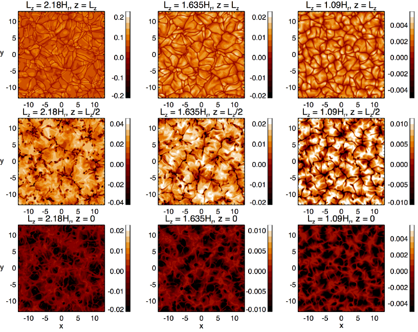
Figure 1: Contour of entropy ($s_{1}$). The three panels in the left, middle, and right columns correspond to the results of cases 1, 2, and 3, respectively. The rows in the top, middle and bottom columns show the plot at $z=L_{z}$, $L_{z}/2$, and $0$, respectively.

Figure 1 shows the results of our hydrodynamic calculation. The three panels in the left, middle and right columns show the contours of entropy in cases 1, 2 and 3, respectively. Due to the large Rayleigh number, the velocity with a large box size is high (see the third row in Table 1). A detailed investigation of cell size distribution will be reported in our forthcoming paper (Iida et al, in preparation).

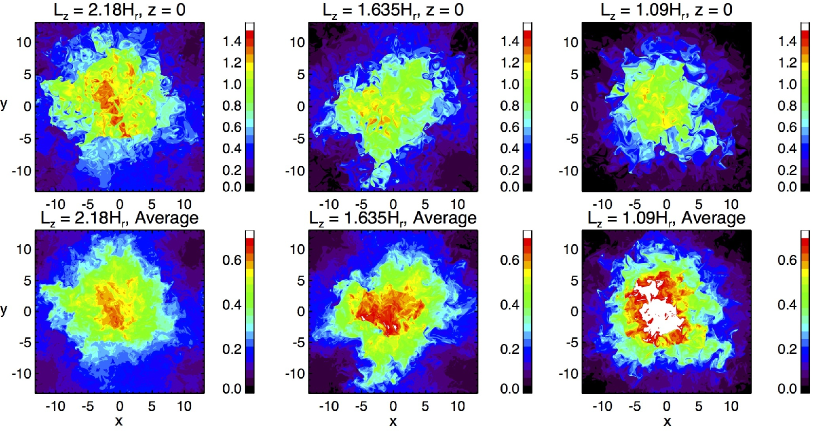
Figure 2: Contour of passive scalar at $t=75H_{\mathrm{r}}/v_{\mathrm{c}}$. The panels in the left, middle, and right columns show the results in cases 1, 2, and 3, respectively. The panels in the top row show the contour of passive scalar $Q$ at $z=0$. The bottom row shows the plot of passive scalar density averaged over $z$, i.e.,$\tilde{Q}$ defined by eq. (19).

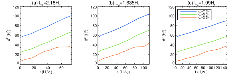
Figure 3: Distribution range $d^{2}$ of the passive scalar as functions of time. Panels a, b, and c show the dependence of $d^{2}$ with the sizes of boxes $L_{z}=2.18H_{\mathrm{r}}$, $1.635H_{\mathrm{r}}$, and $1.09H_{\mathrm{r}}$, respectively. The blue, green, and red lines show the results with $d_{0}=7.5H_{\mathrm{r}}$, $5.0H_{\mathrm{r}}$, and $2.5H_{\mathrm{r}}$, respectively.

Figure 2 shows the contour of the passive scalar whose width of the Gaussian function at the initial condition is $d_{0}=2.5H_{\mathrm{r}}$. We can see that the passive scalar is diffused with turbulent convection. The dependences of $d^{2}$ on $t$ are provided in Figure 3, and are shown to be almost linear. This shows the validity of the diffusive description for the turbulent transport by the convective motion. The estimated turbulent diffusivity is shown in Figure 4a. It is derived through linear fittings to the curves in Figure 3 in the range of $0<t<t_{\mathrm{max}}$ where $t_{\mathrm{max}}$ is chosen so as to reduce the fitting error; it is given in Table 1.

The scaling behavior of the obtained diffusion is studied by changing the depth of the simulation box in cases 1, 2 and 3. In Figure 4a, the blue, green, and red lines show the values of turbulent diffusivity with $d_{0}=7.5H_{\mathrm{r}}$, $5.0H_{\mathrm{r}}$, and $2.5H_{\mathrm{r}}$, respectively. The value of turbulent diffusivity scales with the size of the box, which is discussed in the next paragraph. The value of turbulent diffusivity also scales with the initial width of the Gaussian function $d_{0}$. Using a wider Gaussian function makes the larger size of the convection cell work more efficiently and generates a larger value of turbulent diffusivity.

In the mean field model, it is thought that the coefficient of turbulent diffusion can be expressed as $\eta=L_{\mathrm{c}}v_{\mathrm{rms}}/3$, where $L_{\mathrm{c}}$ is the characteristic length scale of turbulence and $v_{\mathrm{rms}}$ is the root-mean-square (RMS) velocity. The value of turbulent diffusivity is obtained in this study, and we can estimate the value of $L_{\mathrm{c}}$ based on the mean field model i.e., $L_{\mathrm{c}}=3\eta/v_{\mathrm{rms}}$. The estimated horizontal RMS velocities and characteristic length scale are shown in Figure 4b and c, respectively. We discuss the dependence of $L_{\mathrm{c}}$ on the box size with $d_{0}=5.0H_{\mathrm{r}}$ and $7.5H_{\mathrm{r}}$. With a smaller box, i.e. $1.635H_{\mathrm{r}}$ (case 2) and $1.09H_{\mathrm{r}}$ (case 3), the characteristic lengths are almost the same as the sizes of the boxes (the size of the box is indicated by the dashed line). It is natural that the largest cell size is determined by the size of the box and that the largest cell is most effective for advecting the passive scalar. Although we expected that the characteristic length of case 1 would also be the same as $L_{z}$, the obtained characteristic length scale was smaller than $L_{z}$ even with $d_{0}=5.0H_{\mathrm{r}}$ and $7.5H_{\mathrm{r}}$. A possible reason for this result is that the characteristic length $L_{\mathrm{c}}$ is restricted by the convection cell, which is also limited vertically by the pressure scale height ($H_{\mathrm{r}}$) or the density scale height ($\gamma H_{\mathrm{r}}\sim 1.67H_{\mathrm{r}}$). Although $L_{\mathrm{c}}$ should be evaluated in the horizontal scale, the mixture of the passive scalar may occur at approximately the same distance with the vertical scale. It should also be noted that when the narrowest Gaussian function, i.e. $d_{0}=2.5H_{\mathrm{r}}$ (red line), is used, the characteristic lengths are restricted by the width of the Gaussian function in cases 1 and 2.

Next, we discuss the validity of the approximation of turbulent diffusivity quantitatively. We calculate the estimated error of the linear fitting of $d^{2}$ as:

$$\sigma=\sqrt{\frac{1}{N-2}\sum_{n=1}^{N}\left[\frac{d^{2}(t_{n})-\overline{d^{2}(t_{n})}}{\overline{d^{2}(t_{n})}}\right]^{2}},$$ (20)

where $N$ is the number of data points along the time, $d^{2}(t_{n})$ is the $n$-th estimated result and $\overline{d^{2}(t_{n})}$ is the $n$-th result of the fitted line. In Figure 4d, we found a dependence of $\sigma$ on $d_{0}$, i.e. $\sigma$ is larger with narrower $d_{0}$. Although the qualitative relation is not clear, it indicates that the estimated error $\sigma$ tends to become smaller with a larger ratio $d_{0}/L_{\mathrm{c}}$ of the initial width of Gaussian function to the characteristic length (${\bf L_{\mathrm{c}}}$)

4 Summary

We investigated the value of horizontal turbulent diffusivity $\eta$ by a numerical calculation of thermal convection. In this study, we have introduced a new method, whereby the turbulent diffusivity is estimated by monitoring the time development of the passive scalar, which is initially distributed in a given Gaussian function with a spatial scale $d_{0}$. Our conclusions are as follows: (1) Assuming the relation $\eta=L_{\mathrm{c}}v_{\mathrm{rms}}/3$ where $v_{\mathrm{rms}}$ is the RMS velocity, the characteristic length $L_{\mathrm{c}}$ is restricted by the shortest one among the pressure (density) scale height and the region depth. (2) The value of turbulent diffusivity becomes larger with a larger initial distribution scale $d_{0}$. (3) The approximation of turbulent diffusion holds better when the ratio of the initial distribution scale $d_{0}$ to the characteristic length $L_{\mathrm{c}}$ is larger.

Conclusion (2) is consistent with the results of observational study (Chae et al. 2008; Abramenko et al. 2011) and a previous numerical study (Käpylä et al. 2009). In this study, we do not estimate the correlation length directly from the thermal convection. This will be achieved in our future work with an auto-detection technique and our characteristic length ($L_{\mathrm{c}}$) will be compared with directly estimated correlation length. We now assume that our characteristic length is an average of correlation length at each height (Iida et al. in prepareation). The turbulent diffusion in the horizontal directions is estimated in this work, but such estimations are also important in the vertical directions for addressing the solar dynamo problem from the viewpoint of the transport of magnetic flux from the surface to the bottom of the convection zone. Such a study will be conducted in the future.

Although turbulent diffusivity averaged in the whole box is estimated in this study, the dependence of this estimation on the height is important. There are, however, two reasons why it is difficult to estimate this dependence with our method. First, in our calculations the integrated passive scalar density is not conserved at each height. Second, we found that it is difficult to estimate the diffusivity separately for each horizontal plane only by solving eq. (13) two-dimensionally in the $x-y$ plane the because the results show that the passive scalar density is strongly concentrated in the boundaries of the convection cells. Such a spatially intermittent structure is inappropriate for obtaining a statistical property like the turbulent diffusivity. These difficulties will necessitate some substantial improvements in our method. We are also interested in the effect of feedback from the magnetic field to the convection because of its influence on the turbulent diffusivity (e.g. Yousef et al. 2003; Rüdiger et al. 2011).

Table 1: Parameters of study’s calculation.

Case	1	2	3
$L_{x}\times L_{y}\times L_{z}$ $(H_{\mathrm{r}}^{3})$	$26.16^{2}\times 2.18$	$26.16^{2}\times 1.635$	$26.16^{2}\times 1.09$
$N_{x}\times N_{y}\times N_{z}$	$1152^{2}\times 96$	$1152^{2}\times 72$	$1152^{2}\times 48$
$\rho_{0}(L_{z})/\rho_{0}(0)$	22	4.9	2.4
$v_{\mathrm{rms}}$ $(v_{\mathrm{c}})$	0.287	0.206	0.148
$t_{\mathrm{max}}$ $(H_{\mathrm{r}}/v_{\mathrm{c}})$	75	112.5	150

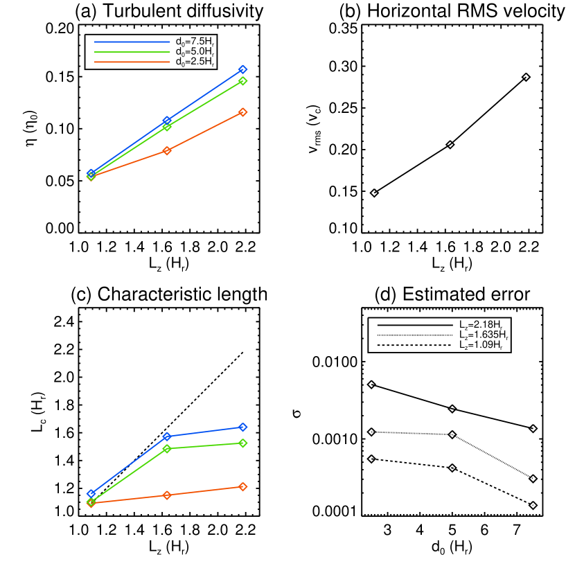
Figure 4: (a) Dependence of turbulent diffusivity on the size of box. The value of turbulent diffusivity is normalized by $\eta_{0}=v_{\mathrm{c}}H_{\mathrm{r}}$ (b) Dependence of horizontal RMS velocity on the size of box. (c) Dependence of characteristic length on size of box. The dashed line shows the size of box. (d) Dependence of estimated error on the width of the Gaussian function. In panels a and b, the blue, green, and red lines show the results with $d_{0}=2.5H_{\mathrm{r}}$, $5.0H_{\mathrm{r}}$, and $7.5H_{\mathrm{r}}$, respectively. In panel d, the solid, dotted and dashed lines show the results with $L_{z}=2.18H_{\mathrm{r}}$, $1.635H_{\mathrm{r}}$, and $1.09H_{\mathrm{r}}$, respectively.

References

- Abramenko et al. (2011) Abramenko, V. I., Carbone, V., Yurchyshyn, V., Goode, P. R., Stein, R. F., Lepreti, F., Capparelli, V., & Vecchio, A. 2011, ApJ, 743, 133
- Brandenburg (2005) Brandenburg, A. 2005, Astronomische Nachrichten, 326, 787
- Brandenburg (2008) —. 2008, Astronomische Nachrichten, 329, 725
- Cameron et al. (2011) Cameron, R., Vögler, A., & Schüssler, M. 2011, A&A, 533, A86
- Chae et al. (2008) Chae, J., Litvinenko, Y. E., & Sakurai, T. 2008, ApJ, 683, 1153
- Choudhuri et al. (2007) Choudhuri, A. R., Chatterjee, P., & Jiang, J. 2007, Physical Review Letters, 98, 131103
- Dikpati & Charbonneau (1999) Dikpati, M., & Charbonneau, P. 1999, ApJ, 518, 508
- Dikpati & Gilman (2006) Dikpati, M., & Gilman, P. A. 2006, ApJ, 649, 498
- Hotta et al. (2012) Hotta, H., Rempel, M., Yokoyama, T., Iida, Y., & Fan, Y. 2012, A&A, 539, A30
- Hotta & Yokoyama (2010a) Hotta, H., & Yokoyama, T. 2010a, ApJ, 709, 1009
- Hotta & Yokoyama (2010b) —. 2010b, ApJ, 714, L308
- Hotta & Yokoyama (2011) —. 2011, ApJ, 740, 12
- Käpylä et al. (2009) Käpylä, P. J., Korpi, M. J., & Brandenburg, A. 2009, A&A, 500, 633
- Miesch (2005) Miesch, M. S. 2005, Living Reviews in Solar Physics, 2, 1
- Rempel (2007) Rempel, M. 2007, ApJ, 655, 651
- Rempel et al. (2009) Rempel, M., Schüssler, M., & Knölker, M. 2009, ApJ, 691, 640
- Rüdiger et al. (2011) Rüdiger, G., Kitchatinov, L. L., & Brandenburg, A. 2011, Sol. Phys., 269, 3
- Rüdiger et al. (2012) Rüdiger, G., Kueker, M., & Schnerr, R. S. 2012, ArXiv e-prints
- Schrinner et al. (2005) Schrinner, M., Rädler, K.-H., Schmitt, D., Rheinhardt, M., & Christensen, U. 2005, Astronomische Nachrichten, 326, 245
- Wang et al. (1989) Wang, Y., Nash, A. G., & Sheeley, Jr., N. R. 1989, ApJ, 347, 529
- Yeates et al. (2008) Yeates, A. R., Nandy, D., & Mackay, D. H. 2008, ApJ, 673, 544
- Yousef et al. (2003) Yousef, T. A., Brandenburg, A., & Rüdiger, G. 2003, A&A, 411, 321