Manifestations of nematic degrees of freedom in the magnetic, elastic, and superconducting properties of the iron pnictides

Abstract

We investigate how emergent nematic order and nematic fluctuations affect several macroscopic properties of both the normal and superconducting states of the iron pnictides. Due to its magnetic origin, long-range nematic order enhances magnetic fluctuations, leaving distinctive signatures in the spin-lattice relaxation rate, the spin-spin correlation function, and the uniform magnetic susceptibility. This enhancement of magnetic excitations is also manifested in the electronic spectral function, where a pseudogap can open at the hot spots of the Fermi surface. In the nematic phase, electrons are scattered by magnetic fluctuations that are anisotropic in momentum space, giving rise to a non-zero resistivity anisotropy whose sign changes between electron-doped and hole-doped compounds. We also show that due to the magneto-elastic coupling, nematic fluctuations soften the shear modulus in the normal state, but harden it in the superconducting state. The latter effect is an indirect consequence of the competition between magnetism and superconductivity, and also causes a suppression of the orthorhombic distortion below $T_{c}$. We also demonstrate that ferro-orbital fluctuations enhance the nematic susceptibility, cooperatively promoting an electronic tetragonal symmetry-breaking. Finally, we argue that $T_{c}$ in the iron pnictides might be enhanced due to nematic fluctuations of magnetic origin.

I Introduction

Understanding the normal state properties of the iron-based superconductors is a key step to decipher the nature of their high-temperature superconducting state (for reviews, see reviews ). In fact, the superconducting (SC) transition temperature $T_{c}$ is maximum near an instability to a spin-density wave state (SDW), suggesting that spin fluctuations may play an important role for the formation of the Cooper pairs magnetic . However, besides this SDW state, another ordered state is observed in the phase diagrams of the iron pnictides: the orthorhombic (Ort) phase. Unlike other superconductors that also display lattice instabilities - such as the cuprates - in the pnictides the Ort transition line always follows the SDW transition line across the phase diagram, even when the latter is bent-back inside the SC dome FernandesPRB10 ; Nandi09 . Most importantly, the Ort transition at $T_{s}$ either precedes or is simultaneous to the SDW transition at $T_{N}$, implying that the lattice distortion is not a mere consequence of long-range magnetic order. Since these two phases are closely related, and since magnetic fluctuations are the main candidate to explain the high-$T_{c}$ SC state, it is natural to investigate in more detail the origin of the Ort phase and its interplay with SC.

On the experimental side, the development of detwinning techniques (see Fisher11 for a review) allowed researchers to investigate the anisotropic properties of the Ort phase using several different experimental probes Chu10 ; Tanatar10 ; Davis10 ; Duzsa11 ; Uchida11 ; Shen11 ; Song11 ; Matsuda11 . It became clear that the small lattice distortion could explain neither the magnitude nor the doping-dependence of these anisotropies - in particular, the remarkable amplitude of the resistivity anisotropy in electron-doped samples Chu10 ; Kuo11 and its sign-change upon hole doping Blomberg12 . Instead, this pool of observations suggest that the Ort phase is actually a manifestation of another electronic ordered phase that breaks the same tetragonal symmetry of the system.

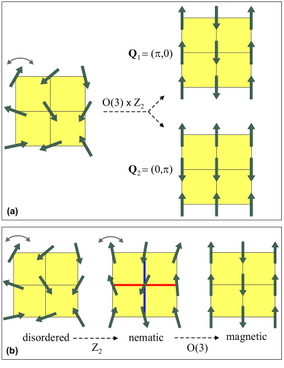
Figure 1: Schematic representation of the nematic transition in real space. (a) The transition from the disordered phase to the SDW phase breaks an $O(3)\times Z_{2}$ symmetry. The $O(3)$ symmetry refers to rotations in spin space while the $Z_{2}$ (Ising) symmetry refers to the two degenerate ground states of magnetic stripes with parallel spins along the $y$ axis (ordering vector $\mathbf{Q}_{1}=\left(\pi,0\right)$) or along the $x$ axis (ordering vector $\mathbf{Q}_{2}=\left(0,\pi\right)$). (b) The $O(3)\times Z_{2}$ symmetry can be broken in two steps. First, only the $Z_{2}$ symmetry is broken: the system is still paramagnetic, since $\left\langle\mathbf{S}_{i}\right\rangle=0$ (indicated by the gray double-arrow on top of the spins), but the spin correlations break the tetragonal symmetry, $\left\langle\mathbf{S}_{i}\cdot\mathbf{S}_{i+\mathbf{x}}\right\rangle=-\left\langle\mathbf{S}_{i}\cdot\mathbf{S}_{i+\mathbf{y}}\right\rangle$ (red and blue bonds, respectively). In the second step, the $O\left(3\right)$ symmetry is broken and the system acquires long-range magnetic order.

On the theoretical side, two different approaches have been proposed to explain the connection between the Ort and SDW phases, as well as the anisotropic properties displayed below $T_{s}$. In one approach, the onset of the SDW is regarded as a consequence of the Ort phase, which itself is driven by a spontaneous ferro-orbital order kruger09 ; RRPSingh09 ; w_ku10 ; Phillips10 ; devereaux10 ; Nevidomskyy11 . In this scenario, the anisotropic properties displayed in the Ort phase are a consequence of the unequal occupations between the $d_{xz}$ and $d_{yz}$ orbitals of the Fe atom. Indeed, a spontaneous orbital polarization is obtained in some (but not all, see Ref. kruger09 ) strong-coupling models - in particular, in some versions of the Kugel-Khomskii model designed for the iron pnictides. However, in weak-coupling or moderate-coupling models, orbital order is usually found only inside the SDW phase, but not as a spontaneous instability of the system preempting the SDW transition bascones ; dagotto ; kotliar .

The other approach adopts the opposite point of view, i.e. that the SDW phase causes the Ort phase Fang08 ; Xu08 ; FernandesPRL10 ; Si08 ; Qi09 ; Mazin09 ; Antropov11 ; JiangpingHu11 ; Batista11 ; Lorenzana_nematic ; FernandesPRB12 . Since $T_{s}\geq T_{N}$, it is not long-range magnetic order, but magnetic fluctuations, that spontaneously break the tetragonal symmetry of the system. Interestingly, similar ideas were proposed in the early 1970s to explain the splitting between the magnetic and the cubic-to-tetragonal transition in a family of rare-earth pnictides, such as DySb, CeSb, DyP, HoP, DyAs Levy71 .

The qualitative idea is simple and can be understood using symmetry arguments, as shown in Fig. 1. In many antiferromagnets, the symmetry that is broken at the magnetic transition temperature is the $O(3)$ spin-rotational symmetry. To the $O(3)$ symmetry breaking corresponds also a translational symmetry breaking, due to the increase in the size of the crystalline unit cell in the magnetically ordered phase. In the iron pnictides, however, the situation is different. The SDW ground state is actually doubly-degenerate, as it is characterized by magnetic stripes of parallel spins along either the $y$ axis (ordering vector $\mathbf{Q}_{1}=\left(\pi,0\right)$) or the $x$ axis (ordering vector $\mathbf{Q}_{2}=\left(0,\pi\right)$). Therefore, to go to the ordered state, the system has to break not only the $O(3)$ spin-rotational symmetry, but it also has to choose between two degenerate ground states, which corresponds to a $Z_{2}$ (Ising-like) symmetry. Since $Z_{2}$ is a discrete symmetry, the $Z_{2}$ symmetry-breaking is expected to be less affected by fluctuations than the continuous $O(3)$ symmetry-breaking, what opens up the possibility of the former happening before the latter.

This is the idea behind the Ising-nematic state: an intermediate phase preempting the SDW state, where the $Z_{2}$ symmetry is broken but the $O(3)$ symmetry is not. In real space, the $Z_{2}$ symmetry-breaking corresponds to a broken tetragonal symmetry, since the correlation functions $\left\langle\mathbf{S}_{i}\cdot\mathbf{S}_{i+\mathbf{x}}\right\rangle$ and $\left\langle\mathbf{S}_{i}\cdot\mathbf{S}_{i+\mathbf{y}}\right\rangle$ acquire opposite signs (see Fig. 1(b)). This is the origin of the term nematic: in liquid crystals, a nematic phase is characterized by a broken rotational symmetry and an unbroken translational symmetry. Although the translational and rotational symmetries are always broken in crystalline solids, the analogy remains valid: in the electronic nematic phase, the point-group symmetry is reduced from $C_{4}$ (tetragonal) to $C_{2}$ (orthorhombic), corresponding to an additional lowering of the rotational symmetry. From a purely symmetry point of view, the nematic state is therefore equivalent to the orthorhombic phase, which is the result of the inevitably induced distortion of the crystalline lattice (see below). The term “nematic” is however used to emphasize the fact that the phase transition is of purely electronic origin and would still take place in a perfectly rigid lattice (for nematic transitions in other systems, see Ref. Fradkin_review ). The recent analysis of Chu et al.IanLegendre demonstrated that it is indeed possible to experimentally determine the driving force behind the transition in the iron pnictides and distinguish between electronic driven transitions and ordinary tetragonal-to-orthogonal structural transitions.

The mechanism behind the spontaneous breaking of the additional Ising symmetry is reminiscent of the order-out-of-disorder mechanism put forward by Chandra, Coleman, and Larkin in the context of localized spin models chandra . Not surprisingly, the first model calculations that obtained an spontaneous nematic phase in the pnictides were based on a strong-coupling approach, the so-called $J_{1}$-$J_{2}$ model Fang08 ; Xu08 ; Si08 . More recently, it was shown that an itinerant description of the system also accounts for a preemptive nematic phase FernandesPRB12 . Notwithstanding important differences between the strong-coupling and weak-coupling approaches - in particular on the character of the nematic and magnetic transitions as function of doping and pressure FernandesPRB12 - they share similar physics: magnetic fluctuations spontaneously break the tetragonal symmetry already in the paramagnetic phase.

In this paper, we will focus not on the origin of the nematic degrees of freedom, but rather on its manifestations in several properties of the iron pnictides, such as the spin-spin correlation function, the spin-lattice relaxation rate, the resistivity anisotropy, the uniform magnetic susceptibility, and the elastic modulus. Since all these quantities are experimentally accessible, they provide important cornerstones to test the predictions of the nematic model. In particular, we will investigate not only the role played by nematic order but also by nematic fluctuations. The former is trivially manifested as a finite orthorhombic distortion of the lattice, but, due to its magnetic origin, it also leaves distinctive signatures in several magnetic properties. For instance, the onset of nematic order enhances magnetic fluctuations, causing a kink in the spin-lattice relaxation rate, and splits the degenerate spectrum of magnetic excitations around $\mathbf{Q}_{1}=\left(\pi,0\right)$ and $\mathbf{Q}_{2}=\left(0,\pi\right)$. Furthermore, we will show that the anisotropic uniform susceptibility and the resistivity anisotropy are proportional to the nematic order parameter near $T_{s}$, although the sign of the latter depends on the geometry of the Fermi surface.

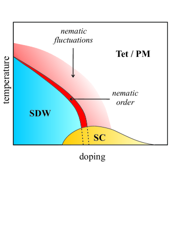
Figure 2: Schematic phase diagram of the iron pnictides, emphasizing the role played by nematic order and nematic fluctuations. SDW denotes the spin-density wave state, SC the superconducting phase, PM the paramagnetic phase, and Tet the tetragonal phase. Tetragonal symmetry is only broken below the nematic/orthorhombic transition line, but nematic fluctuations remain at higher temperatures, as evidenced by shear modulus FernandesPRL10 ; Yoshizawa12 , uniform susceptibility anisotropy Matsuda11 , and resistivity anisotropy Chu10 ; Tanatar10 measurements.

Besides nematic order, low-energy nematic fluctuations also emerge, strongly affecting the system properties. These fluctuations renormalize the shear modulus already at high temperatures, providing a way of probing the nematic susceptibility directly from elastic measurements. We will also discuss the interplay between nematicity and the other electronic degrees of freedom of the system. In particular, we will show how ferro-orbital fluctuations can enhance the tendency to a nematic instability, which in turn can promote orbital order. Finally, the interaction between nematic and superconducting degrees of freedom will be addressed. As a consequence of its magnetic origin and of the competition between SDW and SC, nematicity indirectly competes with SC. This is manifested in the suppression of the orthorhombic distortion below $T_{c}$ and in the hardening of the shear modulus inside the SC dome. Despite this competition, we will give a qualitative argument of why nematic fluctuations can enhance the value of $T_{c}$ without affecting the symmetry of the SC state. The schematic phase diagram shown in Fig. 2 summarizes the main points of this work: not only nematic order, but also nematic fluctuations, play an important role in the physics of the iron pnictides.

The paper is organized as follows: in Section II we review the model that relates the nematic order parameter and the nematic susceptibility to the magnetic spectrum of the system. In Section III we use this model to calculate several system properties that can be probed experimentally: the magnetic properties in the PM-Ort phase (spin-lattice relaxation rate, spin-spin correlation function, and uniform susceptibility); the electronic spectral function in the PM-Ort phase; the orthorhombic distortion in the PM-Ort phase and the shear modulus in the PM-Tet phase; and the resistivity anisotropy above the SDW transition temperature. We address the interplay between nematic and ferro-orbital degrees of freedom in Section IV, while the interplay with superconductivity is investigated in Section V. Section VI is devoted to the conclusions and closing remarks.

II Magnetic model for the nematic phase

We start with an effective action describing the magnetic degrees of freedom Eremin10 ; FernandesPRB12 . Since there are two magnetic ground states, we introduce two order parameters $\mathbf{M}_{1}$ and $\mathbf{M}_{2}$ corresponding respectively to stripes with parallel spins along the $y$ axis (i.e. ordering vector $\mathbf{Q}_{1}=\left(\pi,0\right)$) and stripes with parallel spins along the $x$ axis (i.e. ordering vector $\mathbf{Q}_{2}=\left(0,\pi\right)$). Thus, the spatial magnetic configuration is given by $\mathbf{S}\left(\mathbf{r}\right)=\mathbf{M}_{1}\mathrm{e}^{i\mathbf{Q}_{1}\cdot\mathbf{r}}+\mathbf{M}_{2}\mathrm{e}^{i\mathbf{Q}_{2}\cdot\mathbf{r}}$. The free energy describing these degrees of freedom is given by:

$$F_{\mathrm{mag}} = \int_{q}\chi_{0}^{-1}\left(q\right)\left(\mathbf{M}_{1,q}\cdot\mathbf{M}_{1,-q}+\mathbf{M}_{2,q}\cdot\mathbf{M}_{2,-q}\right)$$ (1)

$$+\frac{u}{2}\int_{x}\left(M_{1}^{2}+M_{2}^{2}\right)^{2}-\frac{g}{2}\int_{x}\left(M_{1}^{2}-M_{2}^{2}\right)^{2}$$

where $\int_{q}=T\sum_{n}\int\frac{d^{d}q}{\left(2\pi\right)^{d}}$ and $q=\left(\mathbf{q},\omega_{n}\right)$ denotes the momentum $\mathbf{q}$ and the Matsubara frequency $\omega_{n}=2n\pi T$. Here $\chi_{0}^{-1}\left(q\right)=r_{0}+q^{2}+\gamma^{-1}\left|\omega_{n}\right|$ is the bare dynamic spin susceptibility and $r_{0}\propto\left(T-T_{N,0}\right)$, with $T_{N,0}$ the mean-field SDW transition temperature and $\gamma$ the Landau damping. Notice that $\mathbf{M}_{i,q}$ is a function of both momentum and Matsubara frequency, as it has both static and dynamic fluctuations.

The coupling constants $u$ and $g$ determine the nature of the magnetic ground state. Consider, for instance, the uniform limit and minimize the free energy $F$ with respect to $M_{i}$. Then, if $g>0$ and $u>0$, we obtain two solutions for $T<T_{N,0}$ corresponding to $M_{2}=0$ and $M_{1}=\sqrt{-r_{0}/u}$ or $M_{1}=0$ and $M_{2}=\sqrt{-r_{0}/u}$. These are nothing but the two degenerate magnetic stripe configurations we discussed earlier. Therefore, hereafter we consider $u>0$ and $g>0$. From symmetry considerations, the action (1) can also contain the term $\left(\mathbf{M}_{1}\cdot\mathbf{M}_{2}\right)^{2}$, which, for $g>0$, does not affect the selection of the ground state as long as its coefficient is not a large negative number compared to $g$.

Although here we introduced the free energy (1) in a phenomenological way, it can be derived microscopically from both the itinerant FernandesPRB12 and localized-spin approaches Fang08 . In both cases, the term $\left(\mathbf{M}_{1}\cdot\mathbf{M}_{2}\right)^{2}$ is absent. Even though both approaches find $g>0$, which selects the magnetic ground states observed in the iron pnictides, the magnitude of this coupling constant is different in the band model and in the $J_{1}-J_{2}$ model. In particular, while in the latter $g$ is small and induced by thermal or quantum fluctuations, in the former it can be large, as it is given by products of the non-interacting electronics Green’s functions. It has been suggested that a relatively large $g$ is necessary in order to fit the spin-wave spectrum inside the SDW phase Antropov11 .

In terms of the magnetic degrees of freedom, the nematic order parameter can be expressed as $\varphi\propto M_{1}^{2}-M_{2}^{2}$. Indeed, $\left\langle\varphi\right\rangle\neq 0$ implies that the fluctuations around one of the ordering vectors $\left\langle M_{1}^{2}\right\rangle$ are on average different than the fluctuations around the other ordering vector $\left\langle M_{2}^{2}\right\rangle$. Since $\mathbf{Q}_{1}=\left(\pi,0\right)$ and $\mathbf{Q}_{2}=\left(0,\pi\right)$ are related by a $90^{\circ}$ rotation in the square-lattice unit cell, $\left\langle M_{1}^{2}\right\rangle\neq\left\langle M_{2}^{2}\right\rangle$ implies that the $x$ and $y$ directions are inequivalent and the tetragonal symmetry is broken. This tetragonal symmetry-breaking is enforced by magnetic fluctuations, and not long-range magnetic order, since $\left\langle M_{1}^{2}\right\rangle\neq\left\langle M_{2}^{2}\right\rangle$ does not require or implies $\left\langle\mathbf{M}_{i}\right\rangle=0$.

Once long-range nematic order sets in, it has a feedback effect on the magnetic fluctuations, assisting the transition to the SDW state. Physically, the nematic order parameter “transfers” magnetic spectral weight from one ordering vector to the other, enhancing magnetic fluctuations in one channel but suppressing them on the other (see Section IIIC). This process increases the SDW transition temperature, as it becomes larger than what it would be in the absence of long-range nematic order.

The expressions relating the nematic order parameter $\varphi$ and the magnetic susceptibility can be obtained by introducing two auxiliary Hubbard-Stratonovich fields in the free energy (1), one for each quartic term (for more details, see FernandesPRB12 ). The first one accounts for the Gaussian fluctuations of the magnetic order parameter, $\left\langle M_{1}^{2}+M_{2}^{2}\right\rangle$, whereas the second one accounts for the possibility of a finite nematic order parameter, $\left\langle M_{1}^{2}-M_{2}^{2}\right\rangle$. In the saddle-point ($1/N$) approximation comment , one obtains a set of non-linear coupled equations for these two auxiliary fields:

$$\varphi = \frac{g}{2}\int_{q}\left[\tilde{\chi}_{1}\left(q\right)-\tilde{\chi}_{2}\left(q\right)\right]$$

$$r = r_{0}+\frac{u}{2}\int_{q}\left[\tilde{\chi}_{1}\left(q\right)+\tilde{\chi}_{2}\left(q\right)\right]$$ (2)

where $r\propto\xi^{-2}$, with $\xi$ denoting the magnetic correlation length renormalized by Gaussian fluctuations. $\tilde{\chi}_{i}\left(q\right)$ is the renormalized magnetic susceptibility at the ordering vector $\mathbf{Q}_{i}$:

$$\tilde{\chi}_{1}\left(q\right) = \frac{1}{\left(r-\varphi\right)+q^{2}+\gamma^{-1}\left|\omega_{n}\right|}$$

$$\tilde{\chi}_{2}\left(q\right) = \frac{1}{\left(r+\varphi\right)+q^{2}+\gamma^{-1}\left|\omega_{n}\right|}$$ (3)

Expanding equations (2) for small $\varphi$, we obtain a familiar $\phi^{4}$-type equation of state for $\varphi$:

$$\left(1-g\int_{q}\chi^{2}\left(q\right)\right)\varphi+b\varphi^{3}+\mathcal{O}\left(\varphi^{5}\right)=0$$ (4)

where $\chi\left(q\right)$ has the same form as the bare susceptibility $\chi_{0}\left(q\right)$ but with $r_{0}$ replaced by $r$, i.e. $\chi^{-1}\left(q\right)=r+q^{2}+\gamma^{-1}\left|\omega_{n}\right|$. The sign of the cubic coefficient $b$ depends on the ratio $u/g$ and on the dimensionality $d$ FernandesPRB12 , and determines whether the nematic transition is first-order or second-order.

For $b>0$, the sign of the linear coefficient determines when a finite $\varphi\neq 0$ becomes a solution of the equation of state (4). At high enough temperatures, the magnetic fluctuations are weak and $\int_{q}\chi^{2}\left(q\right)\propto\xi^{4-d}$ is small, implying that the linear coefficient is positive. Near a magnetic instability, however, $\int_{q}\chi^{2}\left(q\right)$ increases significantly, since it diverges at the magnetic transition temperature for $d+z\leq 4$ ($z$ is the dynamic critical exponent, relevant for quantum phase transitions). Therefore, proximity to an SDW transition makes the linear coefficient change sign, inducing the nematic phase transition. Notice that, for $b<0$, the first-order transition may take place while the linear coefficient is still positive.

Another way of expressing the same results is via the nematic susceptibility, defined as the correlation function $\chi_{\mathrm{nem}}\left(q\right)=\left\langle\left(M_{1}^{2}-M_{2}^{2}\right)_{q}\left(M_{1}^{2}-M_{2}^{2}\right)_{-q}\right\rangle$. After introducing a symmetry-breaking term $h\left(M_{1}^{2}-M_{2}^{2}\right)$ in the free energy (1) and then taking $h\rightarrow 0$, we obtain:

$$\chi_{\mathrm{nem}}=\frac{1}{g}\left(\frac{\left\langle\varphi^{2}\right\rangle}{g}-1\right)$$ (5)

In the saddle-point approximation, it follows that FernandesPRL10 :

$$\chi_{\mathrm{nem}}=\frac{\int_{q}\chi^{2}\left(q\right)}{1-g\int_{q}\chi^{2}\left(q\right)}$$ (6)

As expected, the condition for the onset of long-range magnetic order, $\chi_{\mathrm{nem}}\rightarrow\infty$, agrees with the condition for a finite $\varphi\neq 0$ in the equation of state (4).

It is interesting to obtain a more microscopic understanding of the nematic susceptibility in terms of the electrons. For this, we consider the states around the center of the square-lattice Brillouin zone (annihilation operator $c_{\mathbf{k}}$), where the hole pockets are present, and the states $c_{\mathbf{k}+\mathbf{Q}_{i}}$ in the electron pockets centered at the the magnetic ordering vectors $\mathbf{Q}_{1}=\left(\pi,0\right)$ and $\mathbf{Q}_{2}=\left(0,\pi\right)$. The basic nematic vertex is given by $\varphi\left(M_{1}^{2}-M_{2}^{2}\right)$, and the collective spin modes are expressed in terms of the electronic operators as $\mathbf{M}_{i}=\sum_{\mathbf{k}}c_{\mathbf{k}\alpha}^{\dagger}\bm{\sigma}_{\alpha\beta}c_{\mathbf{k}+\mathbf{Q}_{i}\beta}$, with Pauli matrices $\bm{\sigma}_{\alpha\beta}$. It is convenient to introduce the two-sublattice Neel vectors $\mathbf{L}_{1}$ and $\mathbf{L}_{2}$, defined as $\mathbf{L}_{1}=\mathbf{M}_{1}+\mathbf{M}_{2}$ and $\mathbf{L}_{2}=\mathbf{M}_{1}-\mathbf{M}_{2}$. Then, it follows that $\mathbf{L}_{i}=\sum_{\mathbf{k}}c_{\mathbf{k}\alpha}^{\dagger}\bm{\sigma}_{\alpha\beta}f_{i,\mathbf{k}\beta}$, where we introduced the fermionic operators $f_{1,\mathbf{k}}=c_{\mathbf{k}+\mathbf{Q}_{1}}+c_{\mathbf{k}+\mathbf{Q}_{2}}$ and $f_{2,\mathbf{k}}=c_{\mathbf{k}+\mathbf{Q}_{1}}-c_{\mathbf{k}+\mathbf{Q}_{2}}$. Within this notation, the nematic vertex becomes $\varphi\left(\mathbf{L}_{1}\cdot\mathbf{L}_{2}\right)$, and the nematic susceptibility is given by an Aslamazov-Larkin type diagram, as shown schematically in Fig. 3.

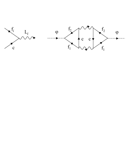
Figure 3: Diagrammatic representation of the nematic susceptibility in terms of the electronic operators $c_{\mathbf{k}}$, $f_{1,\mathbf{k}}=c_{\mathbf{k}+\mathbf{Q}_{1}}+c_{\mathbf{k}+\mathbf{Q}_{2}}$ and $f_{2,\mathbf{k}}=c_{\mathbf{k}+\mathbf{Q}_{1}}-c_{\mathbf{k}+\mathbf{Q}_{2}}$, where $c_{\mathbf{k}}$ is the operator associated with states around the center of the Brillouin zone and $\mathbf{Q}_{i}$ are the magnetic ordering vectors. Dashed lines are the external nematic legs, solid lines are the electronic propagators, and the wavy lines are the magnetic propagators associated with $\mathbf{L}_{1}=\mathbf{M}_{1}+\mathbf{M}_{2}$ and $\mathbf{L}_{2}=\mathbf{M}_{1}-\mathbf{M}_{2}$. The nematic susceptibility (on the right) corresponds to an Aslamazov-Larkin type diagram.

Notice that $\chi_{\mathrm{nem}}$ is a four-spin correlation function. In a regular antiferromagnet, where only one order parameter is present, its critical behavior can be fully expressed in terms of the critical behavior of the two-spin correlation function - the magnetic susceptibility $\chi\left(q\right)$. In that case, the four-spin correlation function does not contain any information that is not already embedded in the two-spin function. In the present case, however, this is not true: due to the nematic degrees of freedom, the four-spin correlation function acquires its own critical behavior, revealing the emergent character of the nematic phase.

In our subsequent analysis we primarily focus on the anomalies that take place at the nematic transition. For a realistic description of the pnictides the behavior at the nearby magnetic transition is of course closely connected to that at the Neel temperature (see Fig. 4). However, in order to stress the behavior of the paramagnetic nematic phase we will frequently consider either two-dimensional systems, where the magnetic ordering temperature is suppressed to zero, or systems where the splitting between the two phase transitions is not too small.

III Manifestations of nematic order and nematic fluctuations in the normal state

One immediate consequence of the coupled non-linear equations (2) is that the nematic and magnetic transitions tend to follow each other. For instance, the divergence of the static nematic susceptibility in Eq. (6) depends on how close the system is to a magnetic instability, where $\int_{q}\chi^{2}\left(q\right)$ diverges. At the same time, once long-range nematic order sets in, the static magnetic susceptibility $\tilde{\chi}_{i}\left(q=0\right)$ is enhanced, as shown in Eq. (3), bringing the SDW transition temperature up. Therefore, both the nematic and the magnetic transitions are tied together, in qualitative agreement with the experimental phase diagrams of the iron pnictides. This is perhaps the most striking feature in favor of the nematic model.

The behavior of the solutions of Eq. (2) has been studied in detail elsewhere, and the characters of the magnetic and nematic transitions have been investigated for a wide range of parameters FernandesPRB12 . In the remainder of the paper, we will focus instead on the manifestations of long-range nematic order, as well as nematic fluctuations, in several properties of the system.

III.1 Orthorhombic distortion: x-ray diffraction

In the nematic model, the spontaneous breaking of the tetragonal symmetry takes place in the magnetic sector, since magnetic fluctuations become stronger around one of the two ordering vectors $\mathbf{Q}_{1}=\left(\pi,0\right)$ and $\mathbf{Q}_{2}=\left(0,\pi\right)$, which are related by a $90^{\circ}$ rotation. Following Landau’s theory of phase transitions, once the tetragonal symmetry is broken in the magnetic sector, it will be broken in all sectors at the same temperature. Indeed, if one constructs another (scalar) order parameter $\eta$ that breaks tetragonal symmetry, it must couple bi-linearly to the nematic order parameter $\varphi$ in the free-energy expansion, implying that $\eta\propto\varphi$ in the free-energy minimum.

This is the case for the orthorhombic order parameter $\varepsilon_{s}\equiv\left(a-b\right)/\left(a+b\right)$, where $a$ and $b$ are the lattice constants. Considering a harmonic lattice, the elastic free energy is given by:

$$F_{\mathrm{el}}=\int_{x}\frac{C_{s}}{2}\,\varepsilon_{s}^{2}-\lambda_{\mathrm{el}}\int_{x}\varepsilon_{s}\left(M_{1}^{2}-M_{2}^{2}\right)$$ (7)

where $C_{s}$ is the shear modulus and $\lambda_{\mathrm{el}}$ is the magneto-elastic coupling. If one works in the coordinate system of the square lattice with one Fe per unit cell, then $C_{s}\equiv C_{11}-C_{12}$; instead, if one works in the coordinate system with two Fe per unit cell, then $C_{s}\equiv C_{66}$. In either case, minimization of Eq. (7) leads to $\varepsilon_{s}\propto\left\langle M_{1}^{2}\right\rangle-\left\langle M_{2}^{2}\right\rangle$, i.e. measuring the orthorhombic distortion is equivalent to measuring the nematic order parameter. Of course, the mere detection of an orthorhombic distortion is by no means an evidence for the electronic character of the structural transition. Yet, one can ask whether there are any signatures of the magnetic character of the structural transition in the behavior of $\varepsilon_{s}$.

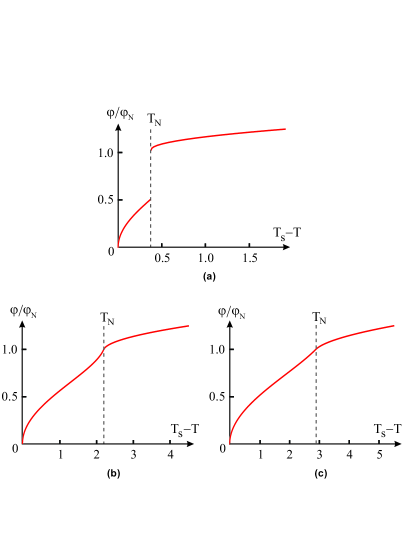
Figure 4: Nematic order parameter $\varphi$ (in units of its value $\varphi_{N}$ at the magnetic transition temperature $T_{N}$) as function of the reduced temperature $T_{s}-T$ (arbitrary units). In panel (a), the split magnetic transition is first-order, while in (b) and (c) it is second-order and progressively farther from the magnetic tricritical point. $\varphi$ is obtained by solving Eqs. (2) for a three-dimensional anisotropic magnetic dispersion. The only parameter changed in each plot is the ratio $u/g$.

Interestingly, the solution of the set of self-consistent equations (2) shows that, when the magnetic and nematic transitions are split, $\varepsilon_{s}$ is in general not affected by the magnetic transition, except near a magnetic tricritical point of the phase diagram FernandesPRB12 . In this region of parameter-space, $\varepsilon_{s}$ has a kink at the magnetic transition temperature - more specifically, $\left|d\varepsilon_{s}/dT\right|_{T_{N}^{-}}<\left|d\varepsilon_{s}/dT\right|_{T_{N}^{+}}$, as shown in Fig. 4. Away from the tricritical point, however, $\varepsilon_{s}$ becomes a smoother function around $T_{N}$. Indeed, x-ray diffraction measurements in $\mathrm{Ba\left(Fe_{1-x}Co_{x}\right)_{2}As_{2}}$ find a kink in the orthorhombic distortion only in the proximity of $x\approx 0.02$ Kim11 , where a magnetic tricritical point has been experimentally established Birgeneau11 .

Notice also that the magneto-elastic coupling has important implications for detwinned samples. Detwinning can be achieved by applying a strain $\varepsilon_{s}$, which acts as an external field to the nematic order parameter $\left\langle M_{1}^{2}\right\rangle-\left\langle M_{2}^{2}\right\rangle$ in Eq. (7), see Ref. IanLegendre . Then, one has to add to the elastic free energy the term $\sigma\varepsilon_{s}$:

$$F_{\mathrm{el}}=\int_{x}\frac{C_{s}}{2}\,\varepsilon_{s}^{2}-\lambda_{\mathrm{el}}\int_{x}\varepsilon_{s}\left(M_{1}^{2}-M_{2}^{2}\right)-\int_{x}\sigma\varepsilon_{s}$$ (8)

For a harmonic lattice, the elastic contribution to the partition function $Z=\int dM_{i}\,d\varepsilon_{s}\mathrm{e}^{-F_{\mathrm{mag}}-F_{\mathrm{el}}}$ can be integrated out analytically, yielding the renormalized magnetic free energy:

$$\tilde{F}_{\mathrm{mag}} = F_{\mathrm{mag}}\left[\mathbf{M}_{1},\mathbf{M}_{2}\right]-\frac{\lambda_{\mathrm{el}}^{2}}{2C_{s}}\int_{x}\left(M_{1}^{2}-M_{2}^{2}\right)^{2}$$ (9)

$$-\frac{\sigma^{2}}{2C_{s}}-\frac{\sigma\lambda_{\mathrm{el}}}{C_{s}}\int_{x}\left(M_{1}^{2}-M_{2}^{2}\right)$$

Comparing to the original action, Eq. (1), the nematic coupling $g$ is enhanced FernandesPRL10 (which holds also for twin samples) and $\sigma$ is converted into an external field for the nematic order parameter, whose amplitude depends on $\lambda_{\mathrm{el}}/C_{s}$. The impact of this external field to the nematic and magnetic transition temperatures has been widely discussed both theoretically Hu12 ; Cano12 and experimentally IanLegendre ; Blomberg11 ; Dhital12 .

III.2 NMR $1/T_{1}T$ spin-lattice relaxation rate

In the nematic model, magnetic fluctuations are responsible for the structural transition. Thus, it is natural to expect that the magnetic properties of the system will undergo noticeable changes at the structural (nematic) transition temperature $T_{s}$. We first study the $1/T_{1}T$ spin-lattice relaxation rate, which can be directly probed by NMR:

$$\frac{1}{T_{1}T}=\gamma_{\mathrm{g}}^{2}\lim_{\omega\rightarrow 0}\sum_{\mathbf{q}}A^{2}\left(\mathbf{q}\right)\frac{\mathrm{Im}\left[\chi_{\mathrm{mag}}\left(\mathbf{q},\omega\right)\right]}{\omega}$$ (10)

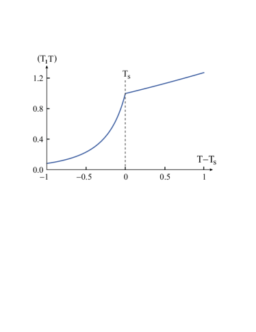
Figure 5: Inverse of the spin-lattice relaxation rate $T_{1}T$ as function of the reduced temperature $T-T_{s}$ for a two-dimensional system. The change in the slope at $T_{s}$ is evident, and should be present whenever the magnetic and structural transitions are split.

Here $\gamma_{\mathrm{g}}$ is the gyromagnetic ratio and $A\left(\mathbf{q}\right)$ is the structure factor of the hyperfine interaction. In our system, $\chi_{\mathrm{mag}}\left(\mathbf{q},\omega\right)$ is strongly peaked at the ordering vectors $\mathbf{Q}_{1}=\left(\pi,0\right)$ and $\mathbf{Q}_{2}=\left(0,\pi\right)$, with $\chi_{\mathrm{mag}}\left(\mathbf{q}+\mathbf{Q}_{i},\omega\right)=\tilde{\chi}_{i}\left(\mathbf{q},\omega_{n}\rightarrow-i\omega+0^{+}\right)$ given by Eqs. (5). Assuming $A\left(\mathbf{q}\right)$ constant, and considering a two-dimensional system for simplicity, we can evaluate the momentum sum around each ordering vector and obtain:

$$\frac{1}{T_{1}T}=\kappa\left(\frac{r}{r^{2}-\varphi^{2}}\right)$$ (11)

where $\kappa>0$ is a constant. In the absence of nematic order, $\varphi=0$, one recovers the usual result $1/T_{1}T\propto 1/\left(T-T_{N}\right)$. However, if the paramagnetic phase undergoes a nematic transition, the spin-lattice relaxation rate diverges when $r=\left|\varphi\right|$, which is the condition for the magnetic transition to take place, see Eq. (5).

Most interestingly, when the nematic/structural and magnetic transitions are split, $1/T_{1}T$ displays a kink at the nematic transition, since:

$$\left(\frac{1}{T_{1}T}\right)_{T_{s}^{-}}-\left(\frac{1}{T_{1}T}\right)_{T_{s}^{+}}\propto\frac{\varphi^{2}}{r^{2}}$$ (12)

In Fig. 5, we illustrate this behavior by presenting the temperature dependence of $T_{1}T$ as calculated from the solution of Eq. (2) at $d=2$. The change of slope at $T_{s}$ is evident. Experimentally, this feature should be more pronounced and easier to observe in compounds with well separated magnetic and structural transitions. Indeed, in NaFeAs, which has $T_{N}\approx 40$ K and $T_{s}\approx 60$ K, NMR measurements Ma_NaFeAs ; kitagawa_NaFeAs have found a very clear change in the slope of $1/T_{1}T$ at $T_{s}$, in agreement with the predictions of the nematic model.

III.3 Spin-spin correlation function: neutron scattering

A more direct probe of the impact of long-range nematic order on the magnetic spectrum can be given by inelastic neutron scattering, as it directly measures the spin-spin correlation function $\mathcal{S}\left(\mathbf{q},\omega\right)=\mathrm{Im}\left[\chi_{\mathrm{mag}}\left(\mathbf{q},\omega\right)\right]/\omega$ at the two ordering vectors $\mathbf{Q}_{1}=\left(\pi,0\right)$ and $\mathbf{Q}_{2}=\left(0,\pi\right)$. In the paramagnetic phase, we have the usual expressions for overdamped spin excitations:

$$\mathcal{S}\left(\mathbf{q}+\mathbf{Q}_{1},\omega\right) =$$

$$\frac{\mathcal{S}_{0}}{\left[\left(r-\varphi\right)+\left(1+\eta\right)q_{x}^{2}+\left(1-\eta\right)q_{y}^{2}\right]^{2}+\gamma^{-2}\omega^{2}}$$ (13)

and:

$$\mathcal{S}\left(\mathbf{q}+\mathbf{Q}_{2},\omega\right) =$$

$$\frac{\mathcal{S}_{0}}{\left[\left(r+\varphi\right)+\left(1-\eta\right)q_{x}^{2}+\left(1+\eta\right)q_{y}^{2}\right]^{2}+\gamma^{-2}\omega^{2}}$$ (14)

with $r\propto\xi^{-2}$ and $\varphi$ solutions of the self-consistent equations (2) and $-1<\eta<1$. These expressions were derived from Eq. (3) with the isotropic magnetic dispersion $q^{2}$ replaced by the anisotropic dispersion $\left(1\pm\eta\right)q_{x}^{2}+\left(1\mp\eta\right)q_{y}^{2}$ , to make comparison with experiments more realistic Diallo10 ; Li10 .

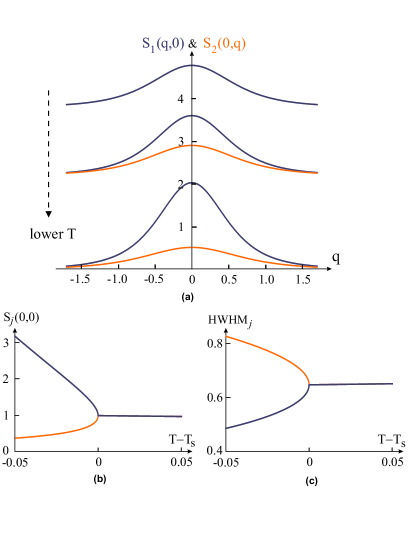
Figure 6: (a) Spin-spin correlation functions $S_{1}\left(q,0\right)\equiv\mathcal{S}\left(q_{x}+\mathbf{Q}_{1},\omega\right)$ (blue) and $S_{2}\left(0,q\right)\equiv\mathcal{S}\left(q_{y}+\mathbf{Q}_{2},\omega\right)$ (orange) as function of momentum transfer $q$ for fixed energy $\omega/\gamma=0.1$ and several temperatures. The upper pairs of curves (coincident) are for a temperature immediately above the structural transition $T_{s}$ while the lower pairs of curves refer to temperatures progressively smaller than $T_{s}$. Here the calculations were done at $d=2$. In (b) and (c), as function of the reduced temperature $T-T_{s}$, we show the $q=0$ peaks and the half-width at half-maximum HWHM of each correlation function $S_{1}\left(q,0\right)$ (blue) and $S_{2}\left(0,q\right)$ (orange).

The nematic order parameter can be obtained by comparing the correlation functions $\mathcal{S}\left(q_{x}+\mathbf{Q}_{1},\omega\right)$ and $\mathcal{S}\left(q_{y}+\mathbf{Q}_{2},\omega\right)$ below $T_{s}$ but still above $T_{N}$ (i.e. in the paramagnetic phase). For a fixed low energy $\omega/\gamma\ll r$, they have peaks at $q=0$ proportional to $\left(r\pm\varphi\right)^{-1}$ and half-widths proportional to $\left(r\pm\varphi\right)^{-1/2}$. In Fig. 6, we plot the temperature evolution of both $\mathcal{S}\left(q_{x}+\mathbf{Q}_{1},\omega\right)$ and $\mathcal{S}\left(q_{y}+\mathbf{Q}_{2},\omega\right)$, as well as the temperature dependence of their peaks and widths. We used the solutions of the self-consistent equations (2) for $d=2$, but the features at $T_{s}$ are of course much more general.

Physically, the onset of long-range nematic order in the paramagnetic phase enhances the magnetic fluctuations around one of the two ordering vectors (in this example, $\mathbf{Q}_{1}$) while suppressing the fluctuations around the other ordering vector ($\mathbf{Q}_{2}$). As a result, the constant-energy cuts of $\mathcal{S}\left(\mathbf{q}+\mathbf{Q}_{1},\omega\right)$ become narrower and stronger, while the constant-energy cuts of $\mathcal{S}\left(\mathbf{q}+\mathbf{Q}_{2},\omega\right)$ become broader and weaker.

A neutron scattering experiment that detects this behavior will provide perhaps the most direct evidence for the magnetic origin of the tetragonal symmetry-breaking in the iron pnictides. Of course, one needs a single crystal that displays split magnetic and structural transitions, such as the 1111 and the 111 compounds, or even some underdoped 122 compounds. The main experimental difficulty is that the crystal needs to be detwinned - i.e. it must have only one structural domain. With the improvement of detwinning techniques, it is reasonable to expect that such an experimental set-up will be available soon.

III.4 Pseudogap in the spectral function: ARPES

In the previous two subsections, we discussed the effects of nematic order on the spectrum of magnetic excitations, and how these effects can be directly probed via magnetic measurements. Another alternative is to probe them indirectly via the electronic spectral function, $A\left(\mathbf{q},\omega\right)=-2\mathrm{Im}\left[G\left(\mathbf{q},\omega\right)\right]$, where $G\left(\mathbf{q},\omega\right)$ is the electronic Green’s function.

Below $T_{N}$, the electronic band structure is reconstructed by long-range magnetic order, and $A\left(\mathbf{q},\omega\right)$ is modified due to the folding of shadow bands and the opening of a SDW gap. Above $T_{N}$, in the paramagnetic phase, the electronic spectral function is affected by magnetic fluctuations. In particular, several works have shown that magnetic precursors are able to reduce the spectral weight of the hot spots at the Fermi level magn_pseudogap . The position $\mathbf{q}_{hs}$ of these hot spots are given by the relation $E\left(\mathbf{q}_{hs}\right)=E\left(\mathbf{q}_{hs}+\mathbf{Q}_{i}\right)$, where $E\left(\mathbf{q}\right)$ denotes the band dispersion. To find the hot spots geometrically, one simply makes a copy of the Fermi surface and displaces it by the magnetic ordering vector $\mathbf{Q}_{i}$: the points that overlap with the original Fermi surface correspond to the hot spots.

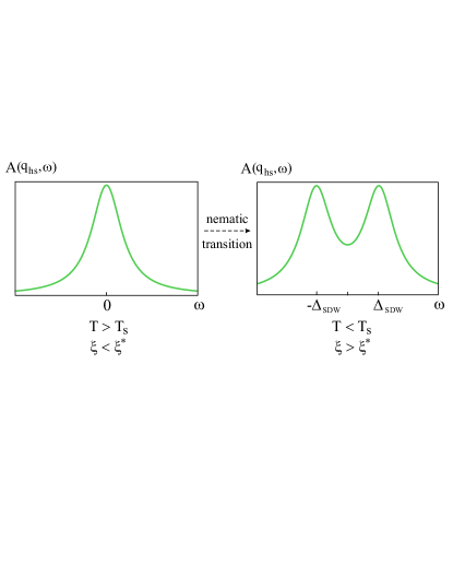
Figure 7: Schematic representation of the opening of a pseudogap in the spectral function $A\left(\mathbf{q}_{hs},\omega\right)$ at the hot spot $\mathbf{q}_{hs}$ due to long-range nematic order. At high temperatures, above the nematic transition temperature $T_{s}$, the magnetic correlation length is below a threshold $\xi^{*}$ and the peak of $A\left(\mathbf{q}_{hs},\omega\right)$ is at $\omega=0$. The onset of nematic order at $T_{s}$ sharply enhances the magnetic fluctuations, as it was shown in Fig. 5, and $\xi$ can overcome $\xi^{*}$. In this case, the maximum of $A\left(\mathbf{q}_{hs},\omega\right)$ shifts to $\omega\approx\Delta_{\mathrm{SDW}}$, which is the SDW gap at $T=0$, and $\omega=0$ becomes a minimum.

Deep inside the magnetically ordered phase, the spectral function at the hot spots vanishes at the Fermi level, i.e. $A\left(\mathbf{q}_{hs},\omega=0\right)=0$. At very high temperatures, $A\left(\mathbf{q}_{hs},\omega\right)$ is maximum at $\omega=0$. At intermediate temperatures in the paramagnetic phase, although $A\left(\mathbf{q}_{hs},\omega=0\right)\neq 0$ always, strong magnetic fluctuations are able to suppress the zero-energy spectral weight at $\mathbf{q}_{hs}$. Above a certain threshold of the magnetic correlation length $\xi$, the maximum at $A\left(\mathbf{q}_{hs},\omega=0\right)$ becomes a minimum as a result of spectral weight being transferred to energies comparable to the zero-temperature SDW gap $\Delta_{\mathrm{SDW}}$, i.e. the maximum is displaced to $A\left(\mathbf{q}_{hs},\omega=\Delta_{\mathrm{SDW}}\right)$, see Fig. 7. Consequently, the electronic spectrum has a pseudogap due to the presence of strong magnetic precursors.

We can now understand how nematic order can affect the electronic spectrum. By sharply enhancing the magnetic fluctuations, as it was shown before in Fig. 5, the onset of long-range nematic order may trigger the opening of a pseudogap at the hot spots of the Fermi surface FernandesPRB12 . In fact, several experiments on the iron pnictides have reported possible manifestations of a pseudogap behavior Tanatar_pseudogap ; Xu_pseudogap , although more work is still necessary to pinpoint its exact temperature scale and its relation to the magnetic and superconducting energy scales. The mechanism proposed here for the pseudogap could be directly probed by ARPES or STM measurements, which are sensitive to the electronic spectral function. Probably the most promising material is NaFeAs, since $T_{s}$ and $T_{N}$ are already below $100$ K and separated by approximately $20$ K.

III.5 Uniform susceptibility: torque magnetometry

Besides affecting the magnetic fluctuations at $\mathbf{Q}_{1}=\left(\pi,0\right)$ and $\mathbf{Q}_{2}=\left(0,\pi\right)$, long-range nematic order also triggers an anisotropy in the uniform magnetic susceptibility $\chi_{\mathrm{mag}}\left(\mathbf{q}=0\right)$. To calculate it, we include the contribution of a non-zero magnetic field $\mathbf{H}$ to the free energy (1) and compare the effects of a field applied along the $x$ direction, $H_{x}$, and a field applied along the $y$ direction, $H_{y}$. We can either use symmetry considerations or perform an explicit calculation by adding the Zeeman term to the electronic dispersions. Neglecting the cross terms $H_{x}H_{y}$, we obtain the general form:

$$F = F_{\mathrm{mag}}\left[\mathbf{M}_{i}\right]+\alpha_{1}\left(H_{x}^{2}+H_{y}^{2}\right)\left(M_{1}^{2}+M_{2}^{2}\right)$$

$$+\alpha_{2}\left[H_{x}^{2}\left(M_{1,x}^{2}+M_{2,x}^{2}\right)+H_{y}^{2}\left(M_{1,y}^{2}+M_{2,y}^{2}\right)\right]$$

with coupling constants $\alpha_{1}$ and $\alpha_{2}$. The first term is isotropic and describes the suppression of SDW order in the presence of an external field. The second term gives an anisotropic response. Since $\chi_{\mathrm{mag}}^{jj}\left(\mathbf{q}=0\right)\propto d^{2}F/dH_{j}^{2}$, we obtain for the anisotropic uniform magnetic susceptibility

$$\chi_{\mathrm{mag}}^{xx}\left(\mathbf{q}=0\right)-\chi_{\mathrm{mag}}^{yy}\left(\mathbf{q}=0\right) \propto$$

$$\left(M_{1,x}^{2}+M_{2,x}^{2}\right)-\left(M_{1,y}^{2}+M_{2,y}^{2}\right)$$ (16)

To understand the anisotropy in the susceptibility, we cannot use the $1/N$ (saddle-point) approach discussed in Section II, since it does not distinguish between the components of the magnetic order parameter. Yet, we can gain qualitative understanding by noting that, in the iron pnictides, the magnetic order parameter points parallel to the modulation axis in the SDW phase, i.e. $\mathbf{M}_{1}\parallel\hat{x}$ while $\mathbf{M}_{2}\parallel\hat{y}$. Therefore, at least within a phenomenological approach, there must be a spin-anisotropy term in the free energy expansion (1) favoring these spin directions. Consequently, the main contribution to the nematic order parameter $\varphi=M_{1}^{2}-M_{2}^{2}$ comes from $\left\langle M_{1,x}^{2}\right\rangle-\left\langle M_{2,y}^{2}\right\rangle$, implying that, to leading order in the spin-anisotropy:

$$\chi_{\mathrm{mag}}^{xx}\left(\mathbf{q}=0\right)-\chi_{\mathrm{mag}}^{yy}\left(\mathbf{q}=0\right)\propto\varphi$$ (17)

Interestingly, recent torque magnetometry experiments on $\mathrm{BaFe_{2}As_{2}}$ and $\mathrm{BaFe_{2}\left(As_{1-x}P_{x}\right)_{2}}$ measured the anisotropy in the uniform magnetic susceptibility, finding a non-zero value below the structural transition temperature Matsuda11 .

III.6 Resistivity anisotropy

The experimental tool that has been mostly used to probe the nematic phase is the resistivity anisotropy $\Delta\rho=\rho_{b}-\rho_{a}$ Chu10 ; Tanatar10 ; Kuo11 ; Blomberg11 . On the theory side, however, unlike the other properties discussed above, $\Delta\rho$ refers to a non-equilibrium situation, what brings additional difficulties to the calculation. Here we follow the same framework of Ref. Fernandes11 and employ a semi-classical Boltzmann equation approach to construct a transport theory for the nematic phase. In this subsection, $b$ and $a$ are parallel to the $y$ and $x$ axis, respectively.

The main property of the nematic phase is that magnetic fluctuations are different around the two ordering vectors $\mathbf{Q}_{1}=\left(\pi,0\right)$ and $\mathbf{Q}_{2}=\left(0,\pi\right)$. The scattering of electrons by these anisotropic spin fluctuations will give rise to an anisotropic scattering rate, resulting in a non-zero resistivity anisotropy $\Delta\rho$ above the magnetic transition temperature $T_{N}$ but below the structural transition temperature $T_{s}$. Of course, below $T_{N}$ the anisotropic reconstruction of the Fermi surface by long-range magnetic order will give another contribution for $\Delta\rho$ bascones ; kotliar , but here we will focus only on the paramagnetic nematic phase.

The electrons that are most efficiently scattered by spin fluctuations are the ones near the hot spots of the Fermi surface, $E\left(\mathbf{q}_{hs}\right)=E\left(\mathbf{q}_{hs}+\mathbf{Q}_{i}\right)$, since they remain near the Fermi level even after acquiring the additional momentum $\mathbf{Q}_{i}$ transferred in the scattering process. The electrons on the other parts of the Fermi surface (called cold regions) do not significantly contribute to the spin-fluctuation scattering. For a very clean system, it was shown in Ref. Hlubina95 that these cold regions of the Fermi surface dominate the transport properties, short-circuiting the contribution from the hot spots. On the other hand, Ref. Rosch99 showed that in dirty systems, the contribution of the spin-fluctuation scattering is the leading-order correction to the residual resistivity $\rho_{0}$. Applying these results to our system, since the resistivity anisotropy comes from the contribution of the hot spots, we expect $\Delta\rho$ to be larger in samples that are dirtier. In fact, this has been recently confirmed by measurements comparing the resistivity anisotropy of normal and annealed samples Uchida11 .

To proceed, we consider the dirty limit where $\rho_{0}$ is large compared to the contribution of the spin-fluctuation scattering. We also consider a three-band model, with a central circular hole pocket $\Gamma$ and two elliptical electron pockets $X$ and $Y$ displaced from the center by the ordering vectors $\mathbf{Q}_{1}=\left(\pi,0\right)$ and $\mathbf{Q}_{2}=\left(0,\pi\right)$, respectively. Due to the tetragonal symmetry of the system, $X$ transforms to $Y$ under a $90^{\circ}$ rotation. Within this model, the resistivity along the $j$ axis is given by (see Ref. Fernandes11 for more details):

$$\frac{\rho_{jj}-\rho_{0}}{\rho_{0}}=c\sum_{\mathbf{q},\mathbf{q}^{\prime}}\sum_{a=X,Y}\,\frac{\left(v_{\Gamma,\mathbf{q}}^{(j)}-v_{a,\mathbf{q}^{\prime}}^{(j)}\right)^{2}}{\omega_{\mathbf{q}-\mathbf{q}^{\prime}}^{(a)}\left(\omega_{\mathbf{q}-\mathbf{q}^{\prime}}^{(a)}+t\right)}$$ (18)

where $t\sim T/\gamma$ is a dimensionless temperature, $v_{a,\mathbf{q}}^{(j)}$ is the $j$-component of the Fermi velocity of band $a$, and $c>0$ is a constant proportional to the ratio between the amplitudes of impurity scattering and spin-fluctuation scattering. Here, $\mathbf{q}$ and $\mathbf{q}^{\prime}$ are momenta restricted to the Fermi surface. The functions $\omega_{\mathbf{q}-\mathbf{q}^{\prime}}^{(a)}$ can be written as $\omega_{\mathbf{q}-\mathbf{q}^{\prime}}^{(a)}=\left(r\pm\varphi\right)+\left|\mathbf{q}_{\Gamma}-\mathbf{q}_{a}^{\prime}-\mathbf{Q}_{a}\right|^{2}$, where the upper (lower) sign refers to band $Y$ ($X$).

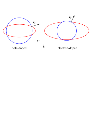
Figure 8: Position of the hot spots in hole-doped and electron-doped compounds. The elliptical electron pocket (red) was displaced by the ordering vector $\mathbf{Q}_{1}=\left(\pi,0\right)$, crossing the circular hole pocket (blue) at the hot spots. The changes in the position of the hot spots are a consequence of the changes in the areas of the electron and hole pockets due to the variation in the charge carrier concentration. We also present the Fermi velocity $\mathbf{v}_{F}=-\mathbf{v}_{\Gamma,\mathbf{q}_{\mathrm{hs}}}$ at the hot spot in each case. Notice that $v_{F}^{(x)}>v_{F}^{(y)}$ in the hole-doped case, whereas $v_{F}^{(y)}>v_{F}^{(x)}$ in the electron-doped case. According to Eq. (19), one expects $\Delta\rho<0$ and $\Delta\rho>0$, respectively.

Performing a $90^{\circ}$ rotation, and using the symmetry properties relating $\mathbf{v}_{X}$ to $\mathbf{v}_{Y}$, we can expand Eq. (18) for small $\varphi$ near the structural transition, obtaining:

$$\frac{\rho_{yy}-\rho_{xx}}{\rho_{0}} = c\,\varphi\sum_{\mathbf{q},\mathbf{q}^{\prime}}\left[\left(v_{\Gamma,\mathbf{q}}^{(y)}-v_{X,\mathbf{q}^{\prime}}^{(y)}\right)^{2}-\left(v_{\Gamma,\mathbf{q}}^{(x)}-v_{X,\mathbf{q}^{\prime}}^{(x)}\right)^{2}\right]$$ (19)

$$\times f\left(\mathbf{q}_{\Gamma}-\mathbf{q}_{X}^{\prime}-\mathbf{Q}_{1}\right)$$

where the function $f\left(\mathbf{k}\right)$ is given by:

$$f\left(\mathbf{k}\right)=\frac{2\left(2k^{2}+2r+t\right)}{\left(k^{2}+r\right)^{2}\left(k^{2}+r+t\right)^{2}}$$ (20)

Therefore, as expected, $\Delta\rho\sim\varphi$, but the sign of the proportionality constant can be positive or negative. Also, $\Delta\rho$ may be small even when $\varphi$ is large (or vice-versa) due to the interplay between impurity-scattering and spin-fluctuation scattering.

The function $f\left(k\right)$ is in general dominated by the $k=0$ contribution - this can be rigorously shown at low temperatures and near an SDW quantum critical point, where $r/t\rightarrow 0$. Thus, the main contribution to the momentum sum comes from $\mathbf{q},\mathbf{q}^{\prime}$ near $\mathbf{q}_{hs},\mathbf{q}_{hs}+\mathbf{Q}_{1}$, and one can obtain the sign of the resistivity anisotropy with respect to $\varphi$ by just analyzing the Fermi velocities of the hot spots.

For instance, if the hot spots are close to the $y$ axis, as it is the case for electron-doped samples Liu10 , then one expects the $y$-component of the Fermi velocity to be larger than the $x$-component, i.e. $\Delta\rho>0$. On the other hand, if the hot spots are close to the $x$ axis, as it is the case for hole-doped samples, the opposite holds and one expects $\Delta\rho<0$ (see Fig. 8). Hence, this general model predicts different signs of $\Delta\rho$ (in the paramagnetic phase) for electron-doped and hole-doped systems. This feature has been recently observed experimentally Blomberg12 , suggesting that the transport properties in the nematic phase are well described by this model of anisotropic spin-fluctuation scattering.

We note that there are other contributions that may affect the resistivity anisotropy in the nematic-paramagnetic phase. For instance, orbital order (see Section IV), which is also induced by nematic order, changes the Drude weight along the $x$ and $y$ directions. Whether this Drude weight redistribution can account for the experimentally observed resistivity anisotropy remains an unsettled issue, as some works find that the resistivity anisotropy coming from this mechanism alone gives the opposite sign of the $\Delta\rho$ measured experimentally Phillips10 ; devereaux10 ; bascones . Impurity effects also play an important role in transport, as discussed above and also in a different model proposed in Ref. kontani_nematic based on orbital order induced by antiferro-orbital fluctuations. A recent Monte Carlo simulation in the spin-fermion model also found that short-range magnetic order (of the same kind that appear in our nematic model) as well as short-range orbital order can promote anisotropic transport Dagotto_Liang .

III.7 Elastic modulus: ultra-sound measurements

So far we discussed several manifestations of long-range nematic order. An interesting question is how one can also probe nematic fluctuations. If these are emergent degrees of freedom of the system, then we expect that their low-energy excitations will have an important effect in the normal state properties.

As we discussed in Section II, nematic fluctuations are four-spin correlation functions, which are rather difficult to measure using standard magnetic probes. An alternative is to investigate how they couple to other degrees of freedom. For instance, Eq. (7) shows that the nematic order parameter acts as a conjugate field to the orthorhombic distortion. Although in the tetragonal phase the mean value of the nematic order parameter is zero, nematic fluctuations are still present. As a result, they will give rise to a quadratic term in the shear distortion $\varepsilon_{s}$ that effectively reduces the shear modulus $C_{s}$. Physically, nematic fluctuations suppress the energy cost of a momentaneous orthorhombic distortion, what is translated as a softening of $C_{s}$. Quantitatively, the renormalized shear modulus is given by:

$$\tilde{C}_{s}^{-1}=\lim_{\sigma\rightarrow 0}\left(\frac{\partial^{2}\ln Z}{\partial\sigma^{2}}\right)$$ (21)

where $Z=\int dM_{i}\,d\varepsilon_{s}\mathrm{e}^{-F_{\mathrm{mag}}-F_{\mathrm{el}}}$ is the partition function, see Eqs. (1) and (8). For a harmonic lattice, the elastic degrees of freedom can be integrated out from the partition function analytically, and we obtain $Z=\int dM_{i}\,\mathrm{e}^{-\tilde{F}_{\mathrm{mag}}}$, with $\tilde{F}_{\mathrm{mag}}$ given by Eq. (9). Taking the derivatives with respect to the infinitesimal stress $\sigma$ and then making $\sigma\rightarrow 0$ we obtain FernandesPRL10 :

$$\tilde{C}_{s}^{-1} = C_{s}^{-1}+\frac{\lambda_{\mathrm{el}}^{2}}{C_{s}^{2}}\,\chi_{\mathrm{nem}}$$

$$\left(\frac{\tilde{C}_{s}}{C_{s}}\right)^{-1} = 1+\frac{\lambda_{\mathrm{el}}^{2}}{C_{s}}\,\chi_{\mathrm{nem}}$$ (22)

where $\chi_{\mathrm{nem}}\left(q\right)=\left\langle\left(M_{1}^{2}-M_{2}^{2}\right)_{q}\left(M_{1}^{2}-M_{2}^{2}\right)_{-q}\right\rangle$, as defined in Section II. Recall that:

$$\chi_{\mathrm{nem}}=\frac{\int_{q}\chi^{2}\left(q\right)}{1-\tilde{g}\int_{q}\chi^{2}\left(q\right)}$$ (23)

with renormalized $\tilde{g}=g+\lambda_{\mathrm{el}}^{2}/C_{s}$ (see Eq. 9). As expected, the divergence of the nematic susceptibility leads to the vanishing of the shear modulus.

Most interestingly, Eq. (22) shows that one can experimentally extract $\chi_{\mathrm{nem}}$ by just measuring the shear modulus $\tilde{C}_{s}$ via standard ultra-sound techniques FernandesPRL10 ; Yoshizawa12 . To calculate $\chi_{\mathrm{nem}}$, one can use inelastic neutron scattering data as input, since they provide the parameters of $\chi\left(q\right)=\xi^{-2}+q^{2}+\gamma^{-1}\left|\omega_{n}\right|$. With this procedure, it is possible to establish whether the measured softening of $\tilde{C}_{s}$ agrees with what one would expect if the structural transition was driven by magnetic fluctuations. This procedure was carried on in Ref. FernandesPRL10 , and a very good agreement was found between the measured $\tilde{C}_{s}$ and the calculated $\chi_{\mathrm{nem}}$, based on neutron scattering data.

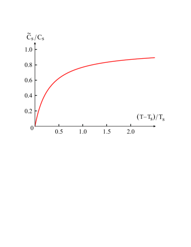
Figure 9: Typical behavior of the shear modulus in the tetragonal phase as function of the reduced temperature. The softening follows Eq. (24); here we used $\kappa=0.3$. The quantity $\tilde{C_{s}}$ is the physical shear modulus, that can be measured in ultra-sound experiments, while $C_{s}$ is its high-temperature limit.

For a finite-temperature nematic transition, $\int_{q}\chi^{2}\left(q\right)\sim\xi^{4-d}\sim\left(T-T_{N,0}\right)^{-\left(4-d\right)\nu}$. Setting $d=2$ and using the mean-field exponent $\nu=1/2$, we obtain a simple expression for the vanishing of the shear modulus:

$$\tilde{C}_{s}=C_{s}\left(1+\kappa\frac{T_{s}}{T-T_{s}}\right)^{-1}$$ (24)

where $\kappa$ is a positive dimensionless constant, of the order of $\kappa\sim\frac{\lambda_{\mathrm{el}}^{2}}{C_{s}\left(E_{\mathrm{mag}}+\tilde{g}\right)}$, with $E_{\mathrm{mag}}$ denoting a characteristic magnetic energy scale. Notice that the shear modulus is reduced to half of its saturation value at $T=T_{s}\left(1+\kappa\right)$. The typical behavior of this function is shown in Fig. 9 and agrees qualitatively well with the experimentally observed softening of $\tilde{C}_{s}$ FernandesPRL10 ; Yoshizawa12 .

IV Nematic order or orbital order?

Besides nematic order, it has been proposed that ferro-orbital order could drive the tetragonal symmetry-breaking observed in the iron pnictides kruger09 ; RRPSingh09 ; w_ku10 ; Phillips10 ; devereaux10 ; Nevidomskyy11 . In this case, the occupation of the Fe $d_{xz}$ orbital is different than the occupation of the $d_{yz}$ orbital. Since the total occupation number depends on all states below the Fermi level, in some cases it is more convenient to refer to the splitting between the on-site orbital energies, $\Delta_{\mathrm{orb}}\equiv\Delta_{xz}-\Delta_{yz}\neq 0$. ARPES measurements have observed $\Delta_{\mathrm{orb}}<0$ in detwinned electron-doped $\mathrm{Ba\left(Fe_{1-x}Co_{x}\right)_{2}As_{2}}$ at the same temperature where a non-zero resistivity anisotropy sets in.

By symmetry, the ferro-orbital order parameter enters the free energy via:

$$F_{\mathrm{orb}}=\int_{x}\frac{\chi_{\mathrm{orb}}^{-1}}{2}\,\Delta_{\mathrm{orb}}^{2}-\lambda_{\mathrm{orb}}\int_{x}\Delta_{\mathrm{orb}}\left(M_{1}^{2}-M_{2}^{2}\right)$$ (25)

where $\chi_{\mathrm{orb}}\equiv\chi_{\mathrm{orb}}\left(q=0\right)$ is the intrinsic ferro-orbital susceptibility, with $\chi_{\mathrm{orb}}\left(q\right)=\left\langle\Delta_{\mathrm{orb}}\left(q\right)\Delta_{\mathrm{orb}}\left(-q\right)\right\rangle$, and $\lambda_{\mathrm{orb}}$ is the appropriate coupling constant to the magnetic degrees of freedom. By minimizing the free energy, it follows that $\Delta_{\mathrm{orb}}\propto\lambda_{\mathrm{orb}}\varphi$. In Ref. FernandesPRB12 , the coupling constant $\lambda_{\mathrm{orb}}$ was calculated using an itinerant approach, and was shown to be negative for electron-doped compounds, providing a possible explanation for why the ARPES measurements observed $\Delta_{\mathrm{orb}}<0$ when $\varphi>0$.

Thus, within the nematic scenario, orbital order is induced by long-range nematic order. However, one could argue that in a model with spontaneous orbital order, where $\chi_{\mathrm{orb}}^{-1}\propto T-T_{\mathrm{orb}}$, orbital order is the one that drives the nematic order. Of course, a phenomenological approach based only on symmetry considerations cannot distinguish between these two different scenarios. One then has to rely on model microscopic calculations to investigate when spontaneous orbital order and/or spontaneous nematic order appear.

In what concerns the nematic scenario, as discussed in Section II, a spontaneous tendency to long-range nematic order is found in both strong-coupling (the $J_{1}-J_{2}$ localized-spin model) and weak-coupling limits (the multi-band nested electronic model). On the other hand, spontaneous ferro-orbital order is mostly found in particular (but not all, see Ref. kruger09 ) versions of the Kugel-Khomskii model, which is obtained in the strong-coupling limit. Furthermore, different numerical analyses of the five-band Hubbard model did not find a ground state that displays orbital order in the absence of long-range magnetic order bascones ; dagotto ; kotliar . Although they do not constitute a proof, these results, combined with the fact that the magnetism in the iron pnictides is closer to the itinerant rather than to the localized-spin regime (since these systems are metallic, see also optical conductivity measurements Wang08 ), suggest that the nematic instability may be the one driving orbital order and structural order.

This does not imply that the role played by the orbital degrees of freedom is irrelevant: for example, it is clear that the reconstruction of the Fermi surface due to orbital order improves the nesting conditions and enhances the magnetic transition temperature Phillips10 ; ZXShen_NaFeAS . The orbital character of the different pockets of the Fermi surface is also important for the superconducting state Zhang09 . Nevertheless, orbital order alone cannot explain the observed anisotropic properties of the iron pnictides. For instance, calculations of the resistivity anisotropy based on the experimentally observed $\Delta_{\mathrm{orb}}<0$ give the opposite sign of the experimental $\rho_{b}-\rho_{a}$ Phillips10 ; devereaux10 ; bascones , indicating that the scattering by anisotropic spin fluctuations is fundamental to explain the observed resistivity anisotropy.

Rather than competing tendencies, ferro-orbital and nematic order are actually cooperative instabilities, which can potentially lead to the enhancement of both the structural transition temperature and the anisotropic properties of the orthorhombic state. To our knowledge, a model that displays both spontaneous nematic and orbital order has not been conceived so far.

Nevertheless, it is clear that there is a coupling between the orbital and magnetic degrees of freedom, since first-principle calculations find that the onset of long-range SDW order is accompanied by ferro-orbital order, due to the different spin polarizations of the $d_{xz}$ and $d_{yz}$ orbitals kotliar . If we assume that the system has a tendency to orbital order, but that $\chi_{\mathrm{orb}}^{-1}>0$ at all temperatures, then we can integrate out the orbital degrees of freedom from the partition function, obtaining the following expression for the nematic susceptibility (see Eq. 23):

$$\chi_{\mathrm{nem}}^{-1}=\left[\int_{q}\chi_{\mathrm{mag}}^{2}\left(q\right)\right]^{-1}-g-\lambda_{\mathrm{orb}}^{2}\,\chi_{\mathrm{orb}}-\lambda_{\mathrm{el}}^{2}\,C_{s}^{-1}$$ (26)

It is clear from this expression how the different degrees of freedom assist nematic fluctuations and nematic order. The first term is just the usual Gaussian fluctuations of the magnetic order parameter, going to zero only at the (bare) magnetic transition temperature. The second term $g>0$ also comes from the magnetic sector (see Eq. 1) and is responsible for the degeneracy of the two magnetic stripe states, i.e. it is the “intrinsic” magnetic instability towards a nematic state. The third term is associated with the orbital degrees of freedom and shows that a tendency towards ferro-orbital order enhances the nematic susceptibility. Finally, the last term, which originates from the magneto-elastic coupling, implies that softer lattices have a larger effective nematic coupling.

V Interplay between nematicity and superconductivity

In the previous sections, we explored the effects of the nematic degrees of freedom on the normal state properties. Here, we investigate how superconductivity and nematic order/fluctuations affect each other.

V.1 Competition with superconducting order

It has been established both experimentally and theoretically that SC and SDW are competing orders in the iron pnictides. Neutron diffraction measurements observe a strong suppression of the SDW order parameter below $T_{c}$ - in some materials, there is even a reentrance of the non-magnetic phase at low temperatures FernandesPRB10 . Theoretically, the fact that the same electrons are responsible for both the static staggered magnetization and the superfluid density explains such a strong competition Fernandes_Schmalian ; Vorontsov10 . In our phenomenological approach, we can capture this competition by adding to the free energy expansion a bi-quadratic SDW-SC term:

$$F\left[\mathbf{M}_{i},\Delta\right]=F_{\mathrm{mag}}\left[\mathbf{M}_{i}\right]+F_{\mathrm{SC}}\left[\Delta\right]+\lambda_{\mathrm{sc}}\left(M_{1}^{2}+M_{2}^{2}\right)\Delta^{2}$$ (27)

In the mean-field level, a non-zero SC order parameter renormalizes the magnetic susceptibility, suppressing the SDW transition temperature $T_{N,0}$:

$$r_{0}\rightarrow r_{0}+\lambda_{\mathrm{sc}}\Delta^{2}$$ (28)

Within this phenomenological approach, it is straightforward to understand qualitatively the effects of superconducting order on the nematic order parameter. Below $T_{c}$, the magnetic susceptibility is suppressed according to Eq. (28). Since long-range nematic order is induced by magnetic fluctuations, it will also be suppressed by SC. This implies that both states are also competing orders, despite the fact that there is no direct coupling between the nematic and SC order parameters.

To investigate the interplay between nematicity and SC quantitatively, we consider the case where the system has no long-range magnetic order once SC sets in. First we analyze the behavior of the nematic order parameter $\varphi$, i.e. we assume $T_{c}<T_{s}$. For simplicity, we solve the self-consistent equations (2) in $d=2$, since in this case there is no finite-temperature SDW transition. A straightforward calculation leads to an implicit equation for $\tilde{\varphi}=4\pi\varphi/gT_{N}$ (see Ref. FernandesPRB12 ):

$$\tilde{\varphi}\coth\tilde{\varphi}+\frac{u}{g}\,\ln\left(\frac{\tilde{\varphi}}{\sinh\tilde{\varphi}}\right)=\tilde{r}_{0}+\tilde{\lambda}_{\mathrm{sc}}\Delta^{2}$$ (29)

where $\tilde{r}_{0}=\alpha\left(T-T_{N}\right)$ and $\tilde{\lambda}_{\mathrm{sc}}=4\pi\lambda_{\mathrm{sc}}/gT_{N}$. For a fixed value of the ratio $u/g$, it is straightforward to solve the self-consistent equation (29) for $\tilde{\varphi}$. In mean-field, for $T>T_{c}$, we have $\Delta^{2}=0$, whereas for $T<T_{c}$, it holds that $\Delta^{2}=\Delta_{0}^{2}\left(T_{c}-T\right)$. The structural transition temperature takes place at $T_{s}=T_{N}+\alpha^{-1}$. Using Eq. (29), we can evaluate $d\varphi/dT$ for all temperatures, obtaining:

$$\left(\frac{d\varphi}{dT}\right)_{T_{c}<T<T_{s}} = -c$$

$$\left(\frac{d\varphi}{dT}\right)_{T<T_{c}\phantom{<T_{s}}} = -\left(1-\frac{\tilde{\lambda}_{\mathrm{sc}}\Delta_{0}^{2}}{\alpha}\right)c$$ (30)

with $c>0$ a temperature-dependent positive number. Eqs. (30) show that the nematic order parameter is suppressed below $T_{c}$. If the competition between SDW and SC is strong enough, such that $\tilde{\lambda}_{\mathrm{sc}}\Delta_{0}^{2}>\alpha$, then $\frac{d\varphi}{dT}$ changes sign below $T_{c}$, implying that the orthorhombic distortion actually decreases inside the SC state. This opens up the possibility of completely killing the Ort phase at low temperatures, promoting a reentrance of the Tet phase. In Fig. 10, we illustrate these behaviors by plotting the solutions of Eq. (29) as a function of temperature for different values of the coupling constant $\tilde{\lambda}_{\mathrm{sc}}$. The competition between the two order parameters has also been investigated by Ref. Moon11 , where a different approach was employed.

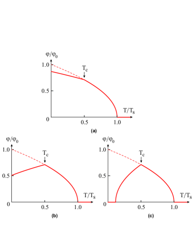
Figure 10: Nematic order parameter $\varphi$ (in units of its zero-temperature value $\varphi_{0}$) as a function of temperature (in units of the structural transition temperature $T_{s}$). The dashed line corresponds to the case with no SC, while the solid line corresponds to the solution in the presence of a SC state that sets in at $T_{c}=T_{s}/2$. The SDW-SC coupling constant was set to $\frac{\tilde{\lambda}_{\mathrm{sc}}\Delta_{0}^{2}}{\alpha}=0.5$ (a), $1.5$ (b) and $2.3$ (c).

Remarkably, x-ray diffraction measurements have found a very strong suppression of the orthorhombic distortion inside the SC phase, and even a reentrance of the tetragonal phase for $\mathrm{Ba\left(Fe_{1-x}Co_{x}\right)_{2}As_{2}}$ near optimal doping Nandi09 . This behavior was observed in the absence of long-range magnetic order, when only the SC and nematic order parameters are non-zero. These measurements provide yet another strong evidence for the electronic character of the structural transition in the iron pnictides, and find a natural explanation within the nematic scenario. No additional coupling between the nematic and SC order parameters is necessary, as the magnetic origin of the nematic phase, combined with the competition between SDW and SC, give rise to an indirect competition between nematicity and SC.

This competition is also manifested in the shear modulus $\tilde{C}_{s}$. An interesting case to analyze is when the system does not have long-range nematic or magnetic order, but only SC at a finite $T_{c}$ (as it is the case in optimally doped samples). For concreteness, we consider the presence of a SDW quantum critical point, such that $r\propto T$. To calculate the shear modulus, we need to evaluate $\int_{q}\chi_{\mathrm{mag}}^{2}\left(q\right)$ in Eq. (23). Above $T_{c}$, we have the usual overdamped spin excitations, $\chi_{\mathrm{mag}}^{-1}\left(q\right)=r+q^{2}+\gamma^{-1}\left|\omega_{n}\right|$. Considering for simplicity $d=2$ and the $T=0$ limit, we obtain:

$$\chi_{\mathrm{nem}}^{-1}=\left[\frac{\gamma}{4\pi^{2}}\ln\left(\frac{\Lambda}{r\gamma}\right)\right]^{-1}-\tilde{g}$$ (31)

where $\Lambda$ is the frequency cutoff. Below $T_{c}$, there are changes not only in the static part of the susceptibility, $r\rightarrow\tilde{r}=r+\lambda_{\mathrm{sc}}\Delta^{2}$, but also in the dynamics of $\chi_{\mathrm{mag}}\left(q\right)$. The presence of a SC gap makes the spin dynamics ballistic for energies $\omega_{n}\ll\Delta$, while for $\omega_{n}\gg\Delta$ one recovers the overdamped dynamics Abanov99 . To capture these two different behaviors, we write the phenomenological form $\chi_{\mathrm{mag}}\left(q\right)=r+q^{2}+f\left(\omega_{n}\right)$ with $f\left(\omega_{n}\right)=\omega_{n}^{2}/\left(\Delta\gamma\right)$ for $\omega_{n}<\Delta$ and $f\left(\omega_{n}\right)=\omega_{n}/\gamma$ for $\omega_{n}>\Delta$. A straightforward calculation then gives:

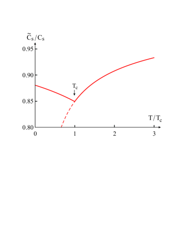
Figure 11: Shear modulus $\tilde{C}_{s}$ (in units of its high-temperature value $C_{s}$) as a function of temperature (in units of $T_{c}$). The dashed line refers to the case without SC and with a putative SDW quantum critical point. The solid line corresponds to the case where SC sets in at $T_{c}$, and reveals the hardening of the shear modulus inside the Tet-SC phase.

$$\chi_{\mathrm{nem}}^{-1}=\frac{4\pi^{2}}{\gamma}\left[\sqrt{\frac{\Delta}{\tilde{r}\gamma}}\arctan\left(\sqrt{\frac{\Delta}{\tilde{r}\gamma}}\right)+\ln\left(\frac{\Lambda}{\tilde{r}\gamma+\Delta}\right)\right]^{-1}-\tilde{g}$$ (32)

with $\tilde{r}=r+\lambda_{\mathrm{sc}}\Delta^{2}$. Substituting this expression in Eq. (22), we obtain the renormalized shear modulus. In Fig. 11, we plot $\tilde{C}_{s}$ using parameters such that $\gamma\gg\Delta$, in accordance to what neutron scattering experiments observe. Notice that the shear modulus is enhanced below $T_{c}$, i.e. the lattice is hardened in the SC phase, due to the suppression of nematic fluctuations. We emphasize that the origin of this behavior is in the magnetic nature of the nematic degrees of freedom, allied to the competition between SDW and SC. The hardening of the shear modulus below $T_{c}$ has been observed by ultra-sound measurements in optimally doped $\mathrm{Ba\left(Fe_{1-x}Co_{x}\right)_{2}As_{2}}$ FernandesPRL10 ; Yoshizawa12 , providing another evidence in favor of the nematic model.

V.2 Nematic fluctuations and superconductivity

Given the evidence in favor of nematic degrees of freedom in the iron pnictides, it is natural to ask whether nematic fluctuations are able to enhance the value of $T_{c}$. Here we give a qualitative argument that this may be the case in the iron pnictides, although more rigorous calculations are necessary to confirm it. We start with a simplified model containing one hole pocket and one electron pocket, both with the same density of states $N_{F}$. The linearized BCS equations for this two-band problem is given by the matrix equation maiti :

$$\left(\begin{array}[]{c}\Delta_{1}\\ \Delta_{2}\end{array}\right)=N_{F}\ln\left(\frac{W}{T_{c}}\right)\left(\begin{array}[]{cc}-U_{1}&-V\\ -V&-U_{2}\end{array}\right)\left(\begin{array}[]{c}\Delta_{1}\\ \Delta_{2}\end{array}\right)$$ (33)

where $W$ is the typical energy scale of the pairing interaction, $U_{1}$ and $U_{2}$ are intra-band interactions, and $V$ is the inter-band interaction. The value of $T_{c}$ is given by the largest eigenvalue $\lambda_{+}$ of the matrix:

$$T_{c}=W\,\mathrm{e}^{-1/\left(N_{F}\lambda_{+}\right)}$$ (34)

If $U_{1}$ and $U_{2}$ are repulsive interactions, i.e. $U_{i}>0$, then SC will only appear if $\left|V\right|>\sqrt{U_{1}U_{2}}$. The largest eigenvalue is given by:

$$\lambda_{+}=-\left(\frac{U_{1}+U_{2}}{2}\right)+\sqrt{\left(\frac{U_{1}-U_{2}}{2}\right)^{2}+V^{2}}$$ (35)

and the eigenvectors give $\Delta_{1}$ and $\Delta_{2}$ with the same sign if $V<0$ (attractive) or $\Delta_{1}$ and $\Delta_{2}$ with opposite signs if $V>0$ (repulsive). In the first case, the SC state is called $s^{++}$ state, while in the second case it is called $s^{+-}$ state. In either case, the interband interaction must be large enough to overcome the intraband repulsion. In the $s^{+-}$ state this becomes possible due to the proximity to a SDW instability, which enhances the interband repulsion $V$ magnetic . The $s^{++}$ state is the leading instability if interband orbital fluctuations (i.e. anti-ferro orbital fluctuations) are strong enough to enhance the electron-phonon attractive interaction orbital . Several experimental results indicate that the state realized in the iron pnictides is the $s^{+-}$. Evidence includes the existence of a resonance mode in the magnetic excitation spectrum below $T_{c}$ Christianson08 ; the pattern of quasi-particle interference in the presence of a magnetic field Hanaguri10 ; half flux-quantum transitions in composite loops of Nb-iron pnictides flux_jumps ; and the microscopic coexistence between SC and SDW FernandesPRB10 .

How nematic fluctuations affect this model? The key point is that, unlike the SDW fluctuations, nematic fluctuations are peaked at $q=0$. Therefore, their main effect should be on the intraband component of the interaction. Moreover, unlike magnetic fluctuations, nematic fluctuations couple to the charge of the electrons. As such, their coupling the electrons is analogous to the coupling between the latter and acoustic phonons, resulting in an attractive intraband interaction $U_{\mathrm{nem}}<0$, i.e. $U_{1}\rightarrow U_{1}-\left|U_{\mathrm{nem}}\right|$. Then, according to Eq. (35), the largest eigenvalue $\lambda_{+}$ would increase and, consequently, $T_{c}$ would be enhanced. Notice that since the pairing interaction due to nematic fluctuations has an intra-band character, it affects $T_{c}$ in the same way regardless of whether the ground state is $s^{++}$ or $s^{+-}$.

Of course, further calculations are necessary to confirm this qualitative picture. One argument that supports a rather weak additional role of nematic-pairing is the absence of significant variations in the gap amplitude on the hole pocket (although recent measurements in LiFeAs found angular variations in the hole-pockets gaps, see LiFeAs_gap ). Notice that the nematic fluctuations would always couple to the form factor $\left(k_{x}^{2}-k_{y}^{2}\right)^{2}$, which should give rise to smaller pairing gaps on the Brillouin zone diagonals. Also, key points neglected in this analysis are the possibility of different frequency cutoffs $W$ among the different interactions and the fact that the nematic coupling should be treated as a quantum critical pairing where all energy scales of the problem contribute to the pairing interaction, not only the ones that are below the typical excitation energy of the nematic mode Abanov01 . Yet, since nematic fluctuations are generated by magnetic fluctuations, it is certainly an interesting open problem to investigate whether this novel collective mode can play a favorable role in Cooper pairing.

VI Concluding remarks

In this paper we discussed distinctive manifestations of the nematic degrees of freedom in several properties of the iron pnictides. Due to the magnetic origin of the nematic phase, magnetic properties such as the spin-lattice relaxation rate, the spin-spin correlation function, and the uniform magnetic susceptibility display characteristic features when the nematic order parameter becomes non-zero at $T_{s}$. Furthermore, the enhancement of magnetic fluctuations at $T_{s}$ also has consequences to the electronic spectrum, opening a pseudogap in the electronic spectral function. Scattering of electrons by these anisotropic spin fluctuations in the nematic paramagnetic phase leads to a resistivity anisotropy whose sign is different in electron-doped and hole-doped compounds.

We also showed that the magneto-elastic coupling makes the orthorhombic distortion proportional to the nematic order parameter, and the shear modulus proportional to the inverse nematic susceptibility. In the normal state, the shear modulus is softened by low-energy nematic fluctuations, but in the SC state it becomes harder due to the indirect competition between nematicity and SC. This indirect competition, rooted on the direct competition between SDW and SC for the same electronic states, is also manifested in the suppression of the orthorhombic distortion below $T_{c}$. The role of orbital order to the onset of long-range nematic order was also discussed. We showed that even when orbital order is not a spontaneous instability of the system, ferro-orbital fluctuations enhance the nematic susceptibility, whose divergence then gives rise to a finite orbital polarization.

It is important to emphasize that, besides orbital order and nematic order, other mechanisms have been proposed for the electronic tetragonal symmetry-breaking in the pnictides. In Ref. zlatko , the authors argue that an orbital-current density wave may be spontaneously generated due to the nesting features of the Fermi surface. As a secondary effect of this orbital-current state, a charge-density wave appears, triggering the structural transition. The authors of Refs. Vojta10 ; Laad11 , on the other hand, suggest proximity to an orbital-selective Mott transition as the origin of the orthorhombic state. Kontani et al. propose an electronic nematic state rooted on quadrupolar orbital interactions allied to impurity effects kontani_nematic . In Ref. daghofer_nematic , Daghofer et al. performed a numerical study of a three-band Hubbard model and found nematic features in the electronic spectral function, although the tetragonal symmetry of the model was explicitly broken by an anisotropic exchange constant. In Ref. Indranil11 , Paul proposes a mechanism for the structural transition based on the magneto-elastic coupling, which is very similar to the emergent nematic model discussed here. We note also that some works treat the coupling between the SDW and structural transitions phenomenologically Cano10 . Such an approach has the clear advantage of providing model-independent predictions, but it does not address why these two transitions follow each other in the phase diagram.

Several of the manifestations of the nematic phase discussed here have been detected experimentally - such as the suppression of the orthorhombic distortion below $T_{c}$ (x-ray diffraction) Nandi09 ; the enhancement of $1/T_{1}T$ below $T_{s}$ (NMR) Ma_NaFeAs ; the anisotropy in the uniform susceptibility (torque magnetometry) Matsuda11 ; the softening of the shear modulus in the normal-Tet phase and its hardening in the SC-Tet phase (ultrasound measurements) FernandesPRL10 ; Yoshizawa12 ; and the change in the sign of the resistivity anisotropy upon hole-doping (transport)Blomberg12 . Yet, there are two important predictions of the nematic model that remain to be seen: the inequivalence between magnetic fluctuations around the ordering vectors $\mathbf{Q}_{1}=\left(\pi,0\right)$ and $\mathbf{Q}_{2}=\left(0,\pi\right)$ below $T_{s}$ (inelastic neutron scattering) and the possible opening of a pseudogap in the electronic spectrum below $T_{s}$ (ARPES and STM). Other manifestations of nematic order not presented here have also been discussed in the literature, such as the effects of nematicity on the SC vortex structure Song11 ; Sachdev_nematic11 , on the elastic domain walls cano_domains , and on the scattering by impurities Davis10 .

Overall, the nematic model offers a simple framework to understand the interplay between the several degrees of freedom present in the phase diagrams of the iron pnictides, shedding light on the primary role played by magnetism. An interesting topic that deserves further attention is the importance of nematic fluctuations to high-temperature SC. Here, we gave a qualitative argument of how $T_{c}$ can be enhanced by nematic fluctuations. A detailed investigation of this result can potentially have implications also for other systems where nematicity has been proposed, such as some cuprates kivelson_cuprates and some heavy fermion systems matsuda_hidden_order .

We would like to thank E. Abrahams, M. Allan, J. Analytis, E. Bascones, A. Böhmer, B. Büchner, P. Canfield, P. Chandra, A. Chubukov, J.-H. Chu, L. Degiorgi, I. Eremin, I. Fisher, A. Goldman, V. Keppens, J. Knolle, A. Kreyssig, R. McQueeney, D. Mandrus, Y. Matsuda, I. Mazin, C. Meingast, A. Millis, S. Nandi, I. Paul, D. Pratt, R. Prozorov, T. Shibauchi, M. Tanatar, and Z. Tesanovic for fruitful discussions. R.F.M. is supported by the NSF Partnerships for International Research and Education (PIRE) program OISE-0968226.

References

- (1) D. C. Johnston, Adv. Phys. 59, 803 (2010); J. Paglione and R. L. Greene, Nature Phys. 6, 645 (2010). P. J. Hirschfeld, M. M. Korshunov, and I. I. Mazin, Rep. Prog. Phys. 74, 124508 (2011); D. N. Basov and A. V. Chubukov, Nature Phys. 7, 241 (2011); P. C. Canfield and S. L. Bud’ko, Annu. Rev. Cond. Mat. Phys. 1, 27 (2010); H. H. Wen and S. Li, Annu. Rev. Cond. Mat. Phys. 2, 121 (2011); A. V. Chubukov, Annu. Rev. Cond. Mat. Phys. 3, 57 (2012); G. R. Stewart, Rev. Mod. Phys. 83 1589 (2011).
- (2) I. I. Mazin, D. J. Singh, M. D. Johannes, and M. H. Du, Phys. Rev. Lett. 101, 057003 (2008); K. Kuroki, S. Onari, R. Arita, H. Usui, Y. Tanaka, H. Kontani, and H. Aoki, Phys. Rev. Lett. 101, 087004 (2008); A. V. Chubukov, D. V. Efremov, and I. Eremin. Phys. Rev. B, 78, 134512 (2008); V. Cvetkovic and Z. Tesanovic, EPL 85, 37002 (2009); R. Sknepnek, G. Samolyuk, Y. Lee, and J. Schmalian, Phys. Rev. B 79, 054511 (2009); A.F. Kemper, T.A. Maier, S. Graser, H-P. Cheng, P.J. Hirschfeld and D.J. Scalapino, New J. Phys. 12, 073030 (2010).
- (3) R. M. Fernandes, D. K. Pratt, W. Tian, J. Zarestky, A. Kreyssig, S. Nandi, M. G. Kim, A. Thaler, N. Ni, P. C. Canfield, R. J. McQueeney, J. Schmalian, and A. I. Goldman, Phys. Rev. B 81, 140501(R) (2010).
- (4) S. Nandi, M. G. Kim, A. Kreyssig, R. M. Fernandes, D. K. Pratt, A. Thaler, N. Ni, S. L. Bud’ko, P. C. Canfield, J. Schmalian, R. J. McQueeney, and A. I. Goldman, Phys. Rev. Lett. 104, 057006 (2010).
- (5) I. R. Fisher, L. Degiorgi, and Z. X. Shen, Rep. Prog. Phys. 74 124506 (2011).
- (6) J.-H. Chu, J. G. Analytis, K. De Greve, P. L. McMahon, Z. Islam, Y. Yamamoto, and I. R. Fisher, Science 329, 824 (2010).
- (7) M. A. Tanatar, E. C. Blomberg, A. Kreyssig, M. G. Kim, N. Ni, A. Thaler, S. L. Bud’ko, P. C. Canfield, A. I. Goldman, I. I. Mazin, and R. Prozorov, Phys. Rev. B 81, 184508 (2010).
- (8) T.-M. Chuang, M. P. Allan, J. Lee, Y. Xie, N. Ni, S. L. Bud’ko, G. S. Boebinger, P. C. Canfield, and J. C. Davis, Science 327, 181 (2010); M. P. Allan et al., unpublished.
- (9) A. Dusza, A. Lucarelli, F. Pfuner, J.-H. Chu, I. R. Fisher, and L. Degiorgi, EPL 93, 37002 (2011); A. Dusza, A. Lucarelli, A. Sanna, S. Massidda, J.-H. Chu, I.R. Fisher, and L. Degiorgi, New J. Phys. 14 023020 (2012).
- (10) M. Nakajima, T. Liang, S. Ishida, Y. Tomioka, K. Kihou, C. H. Lee, A. Iyo, H. Eisaki, T. Kakeshita, T. Ito, and S. Uchida, PNAS 108, 12238 (2011).
- (11) M. Yi, D. Lu, J.-H Chu, J. G. Analytis, A. P. Sorini, A. F. Kemper, B. Moritz, S.-K. Mo, R. G. Moore, M. Hashimoto, W.-S. Lee, Z. Hussain, T. P. Devereaux, I. R. Fisher, and Z.-X. Shen, PNAS 108, 6878 (2011).
- (12) C.-L. Song, Y.-L. Wang, P. Cheng, Y.-P. Jiang, W. Li, T. Zhang, Z. Li, K. He, L. Wang, J.-F. Jia, H.-H. Hung, C. Wu, X. Ma, X. Chen, and Q.-K. Xue, Science 332, 1410 (2011).
- (13) Y. Matsuda et al., unpublished.
- (14) H.-H. Kuo, J.-H. Chu, S. C. Riggs, L. Yu, P. L. McMahon, K. De Greve, Y. Yamamoto, J. G. Analytis, and I. R. Fisher, Phys. Rev. B 84, 054540 (2011).
- (15) E. C. Blomberg, M. A. Tanatar, R. M. Fernandes, Bing Shen, Hai-Hu Wen, J. Schmalian, and R. Prozorov, arXiv:1202.4430.
- (16) F. Krüger, S. Kumar, J. Zaanen, J. van den Brink, Phys. Rev. B 79, 054504 (2009).
- (17) R. R. P. Singh, arXiv:0903.4408.
- (18) C. C. Lee, W. G. Yin, and W. Ku, Phys. Rev. Lett. 103, 267001 (2009); W. G. Yin, C. C. Lee, and W. Ku, Phys. Rev. Lett. 105, 107004 (2010).
- (19) W. Lv, F. Krüger, and P. Phillips, Phys. Rev. B 82, 045125 (2010); W. Lv and P. Phillips, Phys. Rev. B 84, 174512 (2011).
- (20) C.-C. Chen, J. Maciejko, A. P. Sorini, B. Moritz, R. R. P. Singh, and T. P. Devereaux, Phys. Rev. B 82, 100504 (2010); R. Applegate, R. R. P. Singh, C.-C. Chen, and T. P. Devereaux, Phys. Rev. B 85, 054411 (2012).
- (21) A. H. Nevidomskyy, arXiv:1104.1747
- (22) E. Bascones, M. J. Calderon, and B. Valenzuela, Phys. Rev. Lett. 104, 227201 (2010); B. Valenzuela, E. Bascones, and M. J. Calderon, Phys. Rev. Lett. 105, 207202 (2010); M. J. Calderon, G. Leon, B. Valenzuela, and E. Bascones, arXiv:1107.2279
- (23) M. Daghofer, Q. Luo, R. Yu, D. Yao, A. Moreo, and E. Dagotto, Phys. Rev. B 81, 180514(R) (2010); P. M. R. Brydon, M. Daghofer, and C. Timm, J. Phys.: Condens. Matter 23, 246001 (2011); A. Nicholson, Q. Luo, W. Ge, J. Riera, M. Daghofer, G. B. Martins, A. Moreo, and E. Dagotto, Phys. Rev. B 84, 094519 (2011).
- (24) Z. P. Yin, K. Haule, and G. Kotliar, Nature Phys. 7, 294 (2011).
- (25) C. Fang, H. Yao, W.-F. Tsai, J. Hu, and S. A. Kivelson, Phys. Rev. B 77, 224509 (2008).
- (26) C. Xu, M. Müller, and S. Sachdev, Phys. Rev. B 78, 020501(R) (2008).
- (27) R. M. Fernandes, L. H. VanBebber, S. Bhattacharya, P. Chandra, V. Keppens, D. Mandrus, M. A. McGuire, B. C. Sales, A. S. Sefat, and J. Schmalian, Phys. Rev. Lett. 105, 157003 (2010).
- (28) Q. Si and E. Abrahams, Phys. Rev. Lett. 101, 076401 (2008); E. Abrahams and Q. Si, J. Phys.: Condens. Matter 23, 223201 (2011); P. Goswami, R. Yu, Q. Si, and E. Abrahams, Phys. Rev. B 84, 155108 (2011).
- (29) Y. Qi and C. Xu, Phys. Rev. B 80, 094402 (2009).
- (30) I. I. Mazin and M. D. Johannes, Nature Phys. 5, 141 (2009).
- (31) A. L. Wysocki, K. D. Belashchenko, and V. P. Antropov, Nat. Phys. 7, 485 (2011).
- (32) J. Hu, B. Xu, W. Liu, N. Hao, and Y. Wang, arXiv:1106.5169
- (33) Y. Kamiya, N. Kawashima, and C. D. Batista, Phys. Rev. B 84, 214429 (2011).
- (34) M. Capati, M. Grilli, and J. Lorenzana, Phys. Rev. B 84, 214520 (2011).
- (35) R. M. Fernandes, A. V. Chubukov, J. Knolle, I. Eremin, and J. Schmalian, Phys. Rev. B 85, 024534 (2012).
- (36) P. M. Levy and H. H. Chen, Phys. Rev. Lett. 27, 1385 (1971).
- (37) E. Fradkin, S. A. Kivelson, M. J. Lawler, J. P. Eisenstein, and A. P. Mackenzie, Annu. Rev. Condens. Matter Phys. 1, 153 (2010).
- (38) J.-H. Chu, H.-H. Kuo, J. G. Analytis, and I. R. Fisher, arXiv:1203.3239.
- (39) P. Chandra, P. Coleman, and A.I. Larkin, Phys. Rev. Lett. 64, 88 (1990).
- (40) I. Eremin and A. V. Chubukov, Phys. Rev. B 81, 024511 (2010).
- (41) The saddle-point approximation takes into account, in a self-consitent way, the fluctuations of the magnetic order parameter , but not the fluctuations of the Ising order parameter . It is formally valid in the limit , where is the number of components of the magnetic order parameter . For this reason, in the remainder of the text, all relevant coupling constants , , , etc are properly renormalized such that the total action has an overall pre-factor .
- (42) M. G. Kim, R. M. Fernandes, A. Kreyssig, J. W. Kim, A. Thaler, S. L. Bud’ko, P. C. Canfield, R. J. McQueeney, J. Schmalian, and A. I. Goldman, Phys. Rev. B 83, 134522 (2011).
- (43) C. R. Rotundu and R. J. Birgeneau, Phys. Rev. B 84, 092501 (2011).
- (44) J. Hu, C. Setty and S. Kivelson, arXiv:1201.5174.
- (45) A. Cano and I. Paul, arXiv:1201.5594.
- (46) E. C. Blomberg, A. Kreyssig, M. A. Tanatar, R. M. Fernandes, M. G. Kim, A. Thaler, J. Schmalian, S. L. Bud’ko, P. C. Canfield, A. I. Goldman, and R. Prozorov, arXiv:1111.0997.
- (47) C. Dhital, Z. Yamani, W. Tian, J. Zeretsky, A. S. Sefat, Z. Wang, R. J. Birgeneau, and S. D. Wilson, Phys. Rev. Lett. 108, 087001 (2012).
- (48) L. Ma, G. F. Chen, D.-X. Yao, J. Zhang, S. Zhang, T.-L. Xia, and W. Yu, Phys. Rev. B 83, 132501 (2011).
- (49) K. Kitagawa, Y. Mezaki, K. Matsubayashi, Y. Uwatoko, and M. Takigawa, J. Phys. Soc. Jpn. 80, 033705 (2011).
- (50) S. O. Diallo, D. K. Pratt, R.M. Fernandes, W. Tian, J. L. Zarestky, M. Lumsden, T. G. Perring, C. L. Broholm, N. Ni, S. L. Bud’ko, P. C. Canfield, H.-F. Li, D. Vaknin, A. Kreyssig, A .I. Goldman, and R. J. McQueeney, Phys. Rev. B 81, 214407 (2010).
- (51) H.-F. Li, C. Broholm, D. Vaknin, R. M. Fernandes, D. L. Abernathy, M. B. Stone, D. K. Pratt, W. Tian, Y. Qiu, N. Ni, S. O. Diallo, J. L. Zarestky, S. L. Bud’ko, P. C. Canfield, and R. J. McQueeney, Phys. Rev. B 82, 140503(R) (2010).
- (52) M. Vilk and A.-M. S. Tremblay, J. Phys. I France 7, 1309-1368 (1997); J. Schmalian, D. Pines, and B. Stojković, Phys. Rev. Lett. 80, 3839 (1998); Phys. Rev. B 60, 667 (1999); E.Z. Kuchinskii and M. V. Sadovskii, JETP 88, 968 (1999); T. Sedrakyan and A.V. Chubukov, Phys. Rev B 81, 174536 (2010).
- (53) M. A. Tanatar, N. Ni, A. Thaler, S. L. Bud’ko, P. C. Canfield, and R. Prozorov, Phys. Rev. B 82, 134528 (2010).
- (54) Y.-M. Xu, P. Richard, K. Nakayama, T. Kawahara, Y. Sekiba, T. Qian, M. Neupane, S. Souma, T. Sato, T. Takahashi, H.-Q. Luo, H.-H. Wen, G.-F. Chen, N.-L. Wang, Z. Wang, Z. Fang, X. Dai, and H. Ding, Nature Comm. 2, 392 (2011).
- (55) R. M. Fernandes, E. Abrahams, and J. Schmalian, Phys. Rev. Lett. 107, 217002 (2011).
- (56) R. Hlubina and T. M. Rice, Phys. Rev. B 51, 9253 (1995).
- (57) A. Rosch, Phys. Rev. Lett. 82, 4280 (1999).
- (58) C. Liu, T. Kondo, R. M. Fernandes, A. D. Palczewski, E. D. Mun, N. Ni, A. N. Thaler, A. Bostwick, E. Rotenberg, J. Schmalian, S. L. Bud’ko, P. C. Canfield, and A. Kaminski, Nature Phys. 6, 419 (2010).
- (59) S. Liang, G. Alvarez, C. Sen, A. Moreo, and E. Dagotto, arXiv:1111.6994
- (60) M. Yoshizawa, D. Kimura, T. Chiba, A. Ismayil, Y. Nakanishi, K. Kihou, C.-H. Lee, A. Iyo, H. Eisaki, M. Nakajima, and S. Uchida, J. Phys. Soc. Jpn. 81, 024604 (2012).
- (61) W. Z. Hu, J. Dong, G. Li, Z. Li, P. Zheng, G. F. Chen, J. L. Luo, and N. L. Wang, Phys. Rev. Lett. 101, 257005 (2008).
- (62) M. Yi, D. H. Lu, R. G. Moore, K. Kihou, C.-H. Lee, A. Iyo, H. Eisaki, T. Yoshida, A. Fujimori, and Z.-X. Shen, arXiv:1111.6134.
- (63) J. Zhang, R. Sknepnek, R. M. Fernandes, and J. Schmalian, Phys. Rev. B 79, 220502(R) (2009).
- (64) R. M. Fernandes and J. Schmalian, Phys. Rev. B 82, 014520 (2010); ibid Phys. Rev. B 82, 014521 (2010).
- (65) A. B. Vorontsov, M. G. Vavilov, and A. V. Chubukov, Phys. Rev. B 79, 060508(R) (2009); ibid Phys. Rev. B 81, 174538 (2010).
- (66) E. G. Moon and S. Sachdev, arXiv:1112.3973.
- (67) Ar. Abanov and A. V. Chubukov, Phys. Rev. Lett. 83, 1652 (1999).
- (68) S. Maiti, M. M. Korshunov, T. A. Maier, P. J. Hirschfeld, and A. V. Chubukov, Phys. Rev. B 84, 224505 (2011); Phys. Rev. Lett. 107, 147002 (2011).
- (69) S. Onari and H. Kontani, Phys. Rev. Lett. 103, 177001 (2009); H. Kontani and S. Onari, Phys. Rev. Lett. 104, 157001 (2010); Y. Yanagi, Y. Yamakawa, and Y. Ono, Phys. Rev. B 81, 054518 (2010); T. Saito, S. Onari, and H. Kontani Phys. Rev. B 83, 140512(R) (2011).
- (70) A. D. Christianson, E. A. Goremychkin, R. Osborn, S. Rosenkranz, M. D. Lumsden, C. D. Malliakas, I. S. Todorov, H. Claus, D. Y. Chung, M. G. Kanatzidis, R. I. Bewley, and T. Guidi, Nature 456, 930 (2008).
- (71) T. Hanaguri, S. Niitaka, K. Kuroki, and H. Takagi, Science 23, 474 (2010).
- (72) C.-T. Chen, C. C. Tsuei, M. B. Ketchen, Z.-A. Ren, and Z. X. Zhao, Nature Phys. 6, 260 (2010).
- (73) S. V. Borisenko, V. B. Zabolotnyy, A. A. Kordyuk, D. V. Evtushinsky, T. K. Kim, I. V. Morozov, R. Follath, and B. Büchner, Symmetry 4, 251 (2012); M. P. Allan, A. W. Rost, A. P. Mackenzie, Yang Xie, J. C. Davis, K. Kihou, C. H. Lee, A. Iyo, H. Eisaki, and T.-M. Chuang, Science 336, 563 (2012).
- (74) Ar. Abanov, A. V. Chubukov, and J. Schmalian, Europhys. Lett. 55, 369 (2001).
- (75) J. Kang and Z. Tesanovic, Phys. Rev. B 83, 020505 (2011).
- (76) A. Hackl and M. Vojta, New J. Phys. 11, 055064 (2009).
- (77) M. S. Laad and L. Craco, Phys. Rev. B 84, 054530 (2011).
- (78) H. Kontani, T. Saito, and S. Onari, Phys. Rev. B 84, 024528 (2011); Y. Inoue, Y. Yamakawa, and H. Kontani, arXiv:1110.2401.
- (79) M. Daghofer, A. Nicholson, and A. Moreo, arXiv:1202.3656.
- (80) I. Paul, Phys. Rev. Lett. 107, 047004 (2011).
- (81) A. Cano, M. Civelli, I. Eremin, and I. Paul, Phys. Rev. B 82, 020408(R) (2010).
- (82) D. Chowdhury, E. Berg, and S. Sachdev, Phys. Rev. B 84, 205113 (2011).
- (83) A. Cano, Phys. Rev. B 84, 012504 (2011).
- (84) S. A. Kivelson, E. Fradkin, V. Oganesyan, I. P. Bindloss, J. M. Tranquada, A. Kapitulnik, and C. Howald, Rev. Mod. Phys. 75, 1201 (2003).
- (85) R. Okazaki, T. Shibauchi, H. J. Shi, Y. Haga, T. D. Matsuda, E. Yamamoto, Y. Onuki, H. Ikeda, and Y. Matsuda, Science 331, 439 (2011).