Spines of 3-Manifolds as Polyhedra
with Identified Faces

Abstract.

In this article we establish the relation between the spines of 3-manifolds and the polyhedra with identified faces. We do this by showing that the spines of the closed, connected, orientable 3-manifolds can be presented through polyhedra with identified faces in a very natural way. We also prove the equivalence between the special spines and a certain type of polyhedra, and other related results.

0. Introduction

In this article we will consider the polyhedra with identified faces and the spines of 3-manifolds. Spines have been studied broadly by Matveev, among other mathematicians, and their definition, as well as the main theorems concerning them, are available in [8]. Further results on spine theory can be found in [7], [9], [10] and [11]. On the other hand, a polyhedron with identified faces is a solid polyhedron with an even number of polygonal faces, such as a platonic or archimedean solid, in which every $n$-agonal face is identified with another $n$-agonal face in a nice way. Among other things, the identification of two faces has to match up vertices with vertices and edges with edges. Also, the correspondence of the faces must be frontwards. This means that if two identified faces are oriented in an induced way by an arbitrary orientation of the polyhedron, then their identification must be orientation reversing.

Two types of spaces are yielded naturally by these polyhedra. The first one, the space produced by the polyhedron, consists of the space obtained by taking the polyhedron and gluing every face frontwards with the face to which it is identified. The second one, the scar of the polyhedron, is obtained by taking only the boundary of the polyhedron ($S^{2}$) and performing the same gluing. Polyhedra with identified faces are usefull in the study of 3-manifolds because these manifolds can be presented by polyhedra. More specifically, every closed, connected, orientable 3-manifold can be obtained as the space produced by some polyhedron, as it is asserted in Theorem 1.2.

Polyhedra with identified faces are fairly common objects in three-dimentional topology. The lens spaces, for example, are commonly presented by this kind of polyhedra (see [15]). Other examples are the dodecahedron which is the base for constructing the Poincaré’s dodecahedral space, the fundamental domains of isometry groups of $E^{3}$ and $H^{3}$, and the butterflies, developed and studied by Hilden, Montesinos, Tejada, and Toro (see [4], [17]). The methods developed by Montesinos in the study of 3-manifolds as coverings of $S^{3}$ branched over knots have also a close relation with polyhedra with identified faces (see [12], [13]). Some other results concerning this kind of polyhedra can be found in [5] and [14]. However, the study of polyhedra on these works has been mostly lateral, and has been restricted to particular polyhedra or families of these. In spite of its broad applications, polyhedra with identified faces have been rarely defined in a general way or studied independently. This initiative has been undertaken by Cannon, Floyd, and Parry (see [1], [2], [3]) and, from a rather different approach, by the author (see [6]).

The purpose of this article is to establish the relation between the polyhedra with identified faces and the spines of 3-manifolds. This relation is very close since, as we will see, the spines of 3-manifolds can be presented in terms of polyhedra in very convenient ways. This allows us to use polyhedra to define spines and special spines in ways different from the classical one, providing tool in the study of spines.

This presentation of spines through polyhedra is useful for several reasons. In the first place, since any sphere or polyhedron can be seen as a compactified bidimensional Euclidean space, polyhedra with identified faces provide bidimensional descriptions (or diagrams) of spines, being spines intrincated objects of higher dimensions. Besides, complicated mofidications of spines inside the ambient manifolds can be translated into modifications of polyhedra which are very easy to perform (see [6]). Also, since polyhedra are closely related to the presentation of manifolds as branched coverings of $S^{3}$ (see [12], [13]), this work sets a connection between spines and such presentations. Finally, since polyhedra can be frequently embedded on $E^{3}$ and $H^{3}$ nicely (for example when they are fundamental domains, or when they are realized through Andreev’s Theorem), the results proved here suggest the possibility to endow spines with some geometrical meaning.

We can mention also that it has been pointed out by Cannon, Floyd, and Parry that it is very difficult to obtain examples of polyhedra with identified faces that produce 3-manifolds instead of pseudomanifolds (see [1], [2]). In [6] we have already described a method for constructing virtually an unlimited amount of polyhedra that produce 3-manifolds. Here we also approach the problem by identifying a broad family of polyhedra that always produce 3-manifolds (Theorem 2.1).

The structure of the article is as follows. In a first section of preliminary concepts we will introduce briefly the polyhedra with identified faces. A more complete treatment can be found in [6]. In the second section we will show that the set of homogeneous bidimensional spines of closed, connected, orientable 3-manifolds, is exactly the set of scars of the polyhedra that produce such manifolds (Theorem 2.1). Moreover, we will see that a spine of a 3-manifold $M$ can be seen as the scar of a polyhedron that produces that same manifold $M$. In the third section we will define a type of polyhedra that we will call distinguished, and we will prove that the special spines are exactly the scars of the distinguished polyhedra (Theorem 3.5). In the fourth section we will see that distinguished polyhedra are in fact a presentation of the closed, connected, orientable 3-manifolds (Theorem 4.2). In the fifth section we will group the polyhedra into classes, that we will call alikeness classes, and we will prove the equivalence between the alikeness classes of polyhedra and the pairs of the form $(M,S)$, where $M$ is a closed, connected, orientable 3-manifold, and $S$ is a homogeneous bidimensional spine of $M$ (Theorem 5.4). Finally, in the sixth section, we will prove the equivalence between the distinguished polyhedra and the special spines (Theorem 5.4), showing that every special spine can be thought as a distinguished polyhedron and vice versa, and that the presentation of the 3-manifolds by special spines (or special thickenable PL polyhedra) is equivalent to the presentation by distinguished polyhedra.

1. Preliminaries

We begin by fixing some definitions and notation.

Definition 1.

Let $K$ be a CW complex of dimension $n$. We say that $K$ is homogeneous if every cell of dimension less than $n$ is contained in the closure of a cell of higher dimension, and if for every cell $\sigma$ of dimension less than $n-1$, $star(\sigma)-\sigma$ is connected.

Let us notice that a finite homogeneous CW complex of dimension $n$ can be seen in a natural way as a quotient space of $k$ $n$-dimensional closed balls, where $k$ is the number of $n$-dimensional cells in the complex.

Definition 2.

We say that a topological space $G$ is a graph if it can be splitted into open cells in such a way that, if $T$ is the set of these cells, then $\left(G,T\right)$ is a homogeneous one-dimensional CW complex. In this case we also say that $T$ is a triangulation of $G$. We call the zero-dimensional and one-dimensional cells of $T$, respectiveley, the vertices and edges of $G$.

Let us notice that this definition of graph allows what in graph theory is known as loops and multiple edges.

Notation. Given a topological space $X$, we denote the interior and closure of $X$ by $\overset{\circ}{X}$ and $\bar{X}$ respectiveley. Besides, given an arbitrary natural number $m$, we denote by $P_{m}$ the polygon in the complex plane whose vertices are the $m$-th roots of the unit. We understand $P_{2}$ as the unit disk with two vertices at 1 and -1, and we understand $P_{1}$ similarily.

We give now a formal definition of a polyhedron with identified faces. Let $B^{3}$ be the closed three dimensional ball, $G$ a connected graph embedded on $\partial B^{3}$, and $T$ a triangulation of $G$. Then we call the terna $\left\langle B^{3},G,T\right\rangle$ a cell-divided ball. The following lemma is intuitively clear. A proof can be found in [6].

Lemma 1.1.

Let $G$ be as above. Then $\partial B^{3}-G$ is the union of a finite number of disjoint bidimensional open disks.

Let then $\left\langle B^{3},G,T\right\rangle$ be a cell-divided ball such that $\partial B^{3}-G$ consist of $k$ disjoint open disks. We call the vertices and edges of $G$ respectiveley the vertices and edges of $\left\langle B^{3},G,T\right\rangle$, and the clousures of the $k$ mentioned open disks the faces of $\left\langle B^{3},G,T\right\rangle$.

Let us consider now a cell-divided ball $\left\langle B^{3},G,T\right\rangle$ with an even number of faces $k=2n$ oriented in an induced way by an arbitrary orientation of $B^{3}$. And additionally, for each $m\in\mathbb{N}$, let us consider $P_{m}$ with an arbitrary orientation. Now, let us suppose that the $2n$ faces of $\left\langle B^{3},G,T\right\rangle$ can be matched by pairs in such a way that, for each pair $\left\{F_{i},F_{i}^{-1}\right\}$, there exist functions $f_{i}^{+}:P_{m_{i}}\longrightarrow F_{i}$ and $f_{i}^{-}:P_{m_{i}}\longrightarrow F_{i}^{-1}$, where $m_{i}$ is some integer, that satisfy the following conditions:

• Both $f_{i}^{+}$ and $f_{i}^{-}$ restricted $\overset{\circ}{P}_{m_{i}}$ are homeomorphisms.

• Both $f_{i}^{+}$ and $f_{i}^{-}$ send vertices to vertices and edges to edges.

• Of $f_{i}^{+}$ and $f_{i}^{-}$, one preserves the orientation and the other reverses it.

• Both $f_{i}^{+}$ and $f_{i}^{-}$, restricted to any single edge of $P_{m_{i}}$, are PL.

The fourth condition is licit because the edges of $G$ are, naturally, homeomorphic to line segments. We can set then fixed homeomorphisms from $(0,1)$ to each edge of $G$ (And also to the two edges of $P_{2}$ and the single edge of $P_{1}$), and think about these edges as PL polyhedra according to these parametrizations. This way, and since $f_{i}^{+}$ and $f_{i}^{-}$ send edges on edges, we can ask these functions to be PL on the edges of $P_{m_{i}}$.

Now, under these conditions, given a pair of faces $\left\{F_{i},F_{i}^{-1}\right\}$ of $\left\langle B^{3},G,T\right\rangle$, the functions $f_{i}^{+}$ y $f_{i}^{-}$ allow us to define a relation $\epsilon_{i}$ between $F_{i}$ and $F_{i}^{-1}$ under the following rule: $x\in F_{i}$ is related to $y\in F_{i}^{-1}$ if and only if there exists $z\in P_{m_{i}}$ such that $f_{i}^{+}(z)=x$ and $f_{i}^{-}(z)=y$. Taking for each pair of faces the respective relation constructed in this way we get a set of relations $\epsilon:=\{\epsilon_{1},...,\epsilon_{n}\},$ that we will call an identification scheme, for the cell-divided ball $\left\langle B^{3},G,T\right\rangle$. The notation $\epsilon=\{\epsilon_{1},...,\epsilon_{n}\}$ will be recurrent. Let us notice that every $\epsilon_{i}$ is one to one (1-1) on $F_{i}-G$, and at most 2-1 or 1-2 on the edges of $G$. In fact the relation $\epsilon_{i}$ identifies homeomorphically the interior of $F_{i}$ with that of $F_{i}^{-1}$. It also identifies homeomorphically the edges of $F_{i}$ with edges of $F_{i}^{-1}$. However, two edges of $F_{i}$ can eventually be identified with a single edge of $F_{i}^{-1}$, and vice versa.

If $\left\langle B^{3},G,T\right\rangle$ is a cell divided ball and $\epsilon$ is an identification scheme for $\left\langle B^{3},G,T\right\rangle$, we call the quadruple $\left\langle B^{3},G,T,\epsilon\right\rangle$ a polyhedron with identified faces. Throughout this article we will use the word polyhedron to refer to a polyhedron with identified faces, unless otherwise specified. It is worth to notice that there are cell-divided balls for which there does not exist any identification scheme, for example the balls with an odd number of faces. Now, given a polyhedron $\left\langle B^{3},G,T,\epsilon\right\rangle$, the orbits of the points of $\partial B^{3}$ under $\epsilon$ induce an equivalence relation on $\partial B^{3}$, that we denote by $Eq\epsilon$ and call the relation produced by the polyhedron ($Eq\epsilon$ is the smallest equivalence relation that contains the relation $\epsilon_{1}\cup\cdots\cup\epsilon_{n}$). Also, we call the quotient space $B^{3}\diagup Eq\epsilon=B^{3}\diagup\epsilon_{1},...,\epsilon_{n}$ the space produced by the polyhedron.

On the other hand, we have that the relations $\epsilon_{i}$ identify homeomorphically edges with edges. In this way it is possible to take, on the set of edges of $\left\langle B^{3},G,T,\epsilon\right\rangle$, the orbit of a determined edge $a$ under the set of relations $\epsilon$. These orbits are equivalence classes on the set of edges of the polyhedron. Also, this orbits are cyclic, in the sense that $a_{1},...,a_{m}$ form an orbit if and only if there are relations $\epsilon_{i_{1}},...,\epsilon_{im}$ such that $\epsilon_{i_{1}}$ identifies $a_{1}$ with $a_{2}$, $\epsilon_{i_{2}}$ identifies $a_{2}$ with $a_{3}$, … , and $\epsilon_{i_{m}}$ identifies $a_{m}$ with $a_{1}$. Furthermore, there are no other relations on $\epsilon$ other than $\epsilon_{i_{1}},...,\epsilon_{im}$ identifying edges on $\left\{a_{1},...,a_{m}\right\}$.

Similarly, since relations $\epsilon_{i}$ identify vertices with vertices, the orbits of these vertices under $\epsilon$ induce equivlence classes on the set of vertices. Then, given an edge $a$ and a vertex $v$, we call the cardinal of the class of $a$ the cycle of $a$, and the cardinal of the class of $v$ the order of $v$.

At this point we have already a precise definition of a polyhedron with identified faces. However, to ease the later work we shall narrow the definition slightly further, as we will do now.

Definition 3.

Let $X$ be a topological space, and let $r$ and $q$ be two equivalence relations on $X$. We say that $r$ and $q$ are alike if there exists an homeomorphism $f:X\longrightarrow X$  such that for every $x$ and $y$ in $X$, $(x,y)\in r$ if and only if $(f(x),f(y))\in q$. It is easy to see that if $r$ and $q$ are alike, then $f^{\prime}:A\diagup r\longrightarrow A\diagup q$ defined by $f^{\prime}(\left|x\right|)=\left|f(x)\right|$ is an homeomorphism.

Let $\left\langle B^{3},G,T_{1},\epsilon\right\rangle$ and $\left\langle B^{3},H,T_{2},\eta\right\rangle$ be two polyhedra with identified faces. Let us suppose that $Eq\epsilon$ and $Eq\eta$ are alike, and that there exists an homeomorphism $f:\partial B^{3}\longrightarrow\partial B^{3},$ as in definition 3, such that $f(G)=H$. Then on this case we say that $\left\langle B^{3},G,T_{1},\epsilon\right\rangle$ and $\left\langle B^{3},H,T_{2},\eta\right\rangle$ are essentially equal polyhedra. Clearly, essentially equal polyhedra form equivalence classes on the set of polyhedra. Besides, since $f$ is an homeomorphism that “preserves” both the cell-divided structure and the identification scheme, we can assume simply that $G=H$ and $\epsilon=\eta$. Hence, two essentially equal polyhedra are always of the form $\left\langle B^{3},G,T_{1},\epsilon\right\rangle$ and $\left\langle B^{3},G,T_{2},\epsilon\right\rangle$.

Let us consider now the following example. Let $\left\langle B^{3},G,T,\epsilon\right\rangle$ be a polyhedron, and let $\left\{a_{1},...,a_{n}\right\}$ be a class or orbit of edges on $\left\langle B^{3},G,T,\epsilon\right\rangle$. Then we can insert at the middle point of each $a_{i}$ a vertex $v_{i}$, obtaining thus a new triangulation $T_{2}$ of $G$, and a new polyhedron $\left\langle B^{3},G,T_{2},\epsilon\right\rangle$. Let us notice then that $\left\langle B^{3},G,T_{1},\epsilon\right\rangle$ and $\left\langle B^{3},G,T_{2},\epsilon\right\rangle$ are equal in their topological aspects, and differ only because of some redundant vertices. This example insinuates, correctly, that even though triangulations of graphs play an important role in the definition of polyhedra, by determining the edges and vertices of the same, such triangulations are superfluous from a topological point of view. The fact is, as we will see, that essentially equal polyhedra are topologically identical, for which it is desirable to work only with simple class representatives.

We will see now the construction of a standard representative for each class of essentially equal polyhedra. Let $G$ be a graph and $T$ be a triangulation of $G$. Then, we say that a vertex of $(G,T)$ is topologically superfluous if it is adyacent to exactly two edges. Let us consider now a polyhedron $\left\langle B^{3},G,T,\epsilon\right\rangle$, and a vertex $v_{1}$ of $\left\langle B^{3},G,T\right\rangle$. Let us recall that every point in the orbit of $v_{1}$ is also a vertex. We say that $v_{1}$ is a needless vertex in $\left\langle B^{3},G,T,\epsilon\right\rangle$ if the following conditions are satisfied:

• Every point $v_{1},...,v_{n}$ in the orbit of $v_{1}$ is a topologically superfluous vertex of $G$.

• There does not exist an edge of $T$ whose endings belong both to the set $\left\{v_{1},...,v_{n}\right\}$.

It is worth to mention, even when we are not interested in proving it, that (1) implies (2) as long as the space produced by $\left\langle B^{3},G,T,\epsilon\right\rangle$ is not a lens.

Now, let $T_{0}$ be the triangulation obtained by the removal of all the needless vertices of $T$. We call $T_{0}$ the standard triangulation of $\left\langle B^{3},G,T,\epsilon\right\rangle$. The good definition of $T_{0}$ follows inmediately from (1) and (2). Also, we understand that by the elimination of each vertex, the two edges adyacent to it are merged into a single edge.

It can be proved that if $T_{0}$ is the standard triangulation for $\left\langle B^{3},G,T,\epsilon\right\rangle$, then $\left\langle B^{3},G,T_{0},\epsilon\right\rangle$ is a well defined polyhedron. It is clearly seen thus that $\left\langle B^{3},G,T_{0},\epsilon\right\rangle$ is essentially equal to $\left\langle B^{3},G,T,\epsilon\right\rangle$. We call $\left\langle B^{3},G,T_{0},\epsilon\right\rangle$ the standard polyhedron for $\left\langle B^{3},G,T,\epsilon\right\rangle$. It can be seen also that essentially equal polyhedra have the same standard polyhedron, for which we will also say that $\left\langle B^{3},G,T_{0},\epsilon\right\rangle$ is the standard polyhedron for the class of $\left\langle B^{3},G,T,\epsilon\right\rangle$ (More exactly, what we have is that if $\left\langle B^{3},G,T_{1},\epsilon\right\rangle$ and $\left\langle B^{3},G,T_{2},\epsilon\right\rangle$ are essentially equal polyhedra, and if $\left\langle B^{3},G,T_{1,0},\epsilon\right\rangle$ and $\left\langle B^{3},G,T_{2,0},\epsilon\right\rangle$ are their standard polyhedra, then there exists an homeomorphism $f:\partial B^{3}\longrightarrow\partial B^{3}$ as in Definition 3 such that $f(G)=G$, and such that $f\mid_{G}$ is a graph isomorphism)

From now on we will understand essentially equal polyhedra as the same polyhedron. For that reason, instead of working with the set of all polyhedra, we will work with the set of classes of essentially equal polyhedra, or equivalently, the set of standard polyhedra. We will narrow thus our definition of polyhedron with identified faces to include only standard polyhedra, that is, polyhedra without needless vertices.

We will also use the following notation. Let $\left\langle B^{3},G,T_{0},\epsilon\right\rangle$ be the standard polyhedron for the class of a given polyhedron $\left\langle B^{3},G,T,\epsilon\right\rangle$. Such a class, and therefore its standard polyhedron, is determined uniquely by the graph $G$ and the identification scheme $\epsilon$, so we can now denote $\left\langle B^{3},G,T_{0},\epsilon\right\rangle$ simply by $\left\langle B^{3},G,\epsilon\right\rangle$. We will adopt this notation from now on.

We will finish this section by examining what kind of spaces are produced by polyhedra with identified faces. Let $X$ be a compact, connected, second-countable Hausdorff topological space that satisfies the following conditions:

• Every point of $X$, except perhaps a finite number, has a neighborhood homeomorphic to a three dimensional open ball.

• If $x\in X$ has not a neighborhood of this type, it has a neighborhood whose closure is homeomorphic to the cone of a connected sum of tori.

In this case we say that $X$ is a pseudomanifold of type $\mathcal{P}_{1}$, and it can be seen that every pseudomanifold of this type is triangulable (see [6]). We say then that $X$ is of type $\mathcal{P}_{1}o$ if it is orientable, and of type $\mathcal{P}_{1}n$ if it is not. Those points of a pseudomanifold that do not have a neighborhood homeomorphic to a ball, if they exist, are called singularities. We state now a theorem that determines exactly which are the spaces produced by polyhedra with identified faces. We will not prove the theorem, whose proof can be found in [6].

Theorem 1.2.

The set of the spaces produced by polyhedra whith identified faces is exactely the set of pseudomanifolds of type $\mathcal{P}_{1}o$. Besides, if a polyhedron produces a pseudomanifold $P$, and $x$ is a singularity of $P$, then $x$ comes from the identification of vertices in the polyhedron.

In particular, since every closed, connected, orientable 3-manifold is trivially a pseudomanifold of type $\mathcal{P}_{1}o$, we have that for every closed, connected, orientable 3-manifold there exists a polyhedron that produces it. Also, no manifold of other kind can be produced by a polyhedron.

2. Spines and Scars

Given a polyhedron $\left\langle B^{3},G,\epsilon\right\rangle$, we call the space $\partial B^{3}\diagup Eq\epsilon$ the scar of the polyhedron. Let us notice that the scar of a polyhedron is a subspace of the space produced by the same, for $\partial B^{3}\diagup Eq\epsilon\subseteq B^{3}\diagup Eq\epsilon$. Besides, the scar of a polyhedron has a natural homogeneous bidimensional CW complex structure, where each cell is obtained in the following way. Each pair of faces of the polyhedron yields an open $2$-cell or face in the scar, produced when the interior of the faces are glued together. Similarily, each class of $n$ edges of cycle $n$ in the polyhedron yields an open $1$-cell or edge in the scar, produced when the $n$ edges are glued toguether becoming a single one. And finally, each class of $m$ vertices of order $m$ yields a $0$-cell or vertex on the scar in the same way. Let us notice that, since many polyhedra can produce the same scar, the CW complex structure just defined depends on the choice of one of these polyhedra.

Leaving aside scars for a moment, let us recall that every spine of a 3-manifold is a CW complex (For the definition and main properties of spines see [8]). Then we say that a spine is bidimensional if it is homeomorphic to a bidimensional CW complex. Similarily we will say that a spine is homogneous if it is homeomorphic to a homogeneous CW complex.

The goal of this section is to prove the following theorem, which establishes the equivalence between the scars of polyhedra that produce manifolds, and the spines of 3-manifolds that are homogeneous bidimensional CW complexes.

Theorem 2.1.

Let $M$ be a closed, connected, orientable 3-manifold, and $S\subseteq M$. Then, $S$ is a homogeneous bidimensional spine of $M$ if and only if it is the scar of a polyhedron that produces $M$.

Let us begin by recalling some definitions and notations regarding collapses on simplicial complexes. Given a simplicial complex $K$ in $\mathbb{R}^{k}$, we will denote the union of the elements of $K$ by $\left|K\right|$, and the barycentric subdivision of $K$ by $K^{\prime}$. On the other hand, let us recall that if $K$ is a simplicial complex, we say that an $n$-simplex $\sigma^{n}$ in $K$ is principal if it is not a face of any other simplex in $K$ but itself. Additionally, we say that an $(n-1)$-simplex $\rho^{n-1}$ in $K$ is a free face of $\sigma^{n}$ if  it is a face of $\sigma^{n}$, of itself, and of no other simplex. Now, if $\sigma$ is principal in $K$ and $\rho$ is a free face of $\sigma$, we say that the complex $K$ collapses elementally to the subcomplex $K-\{\sigma,\rho\}$, and we write $K\searrow K-\{\sigma,\rho\}$. If $L$ is a subcomplex of $K$, and it is possible to obtain $L$ form $K$ by means of a finite secuence of elementary collapses $K\searrow\cdots\searrow L$, we say that $K$ collapses to $L$, and we write $K\searrow L$ (see [8]).

We shall now prepare the hypotheses necessary to state a lemma that is rather technical, but will be necesarry for a step of the proof of Theorem 2.1. Let $K$ be a finite three dimensional simplicial complex in $\mathbb{R}^{k}$, and $L$ be a bidimensional subcomplex of $K$ with an even number of triangles $l_{1},...,l_{2n}$. On the other hand, for each $1\leq i\leq n$, let $f_{i}:\mathbb{R}^{k}\longrightarrow\mathbb{R}^{k}$ be an affine transformation such that $f_{i}(l_{i})=l_{i+n}$. We will have under consideration the spaces $\left|K\right|\diagup\left\{f_{i}\right\}_{i=1}^{n}$ and $\left|L\right|\diagup\left\{f_{i}\right\}_{i=1}^{n}$.

Let us denote by $\pi$ the projection of $\left|K\right|$ onto $\left|K\right|\diagup\left\{f_{i}\right\}$. Then, if $\left\{T_{i}\right\}$ is the set of simplexes of the second barycentric subdivision of $K$, $K^{\prime\prime}$ (i.e. $\left\{T_{i}\right\}=K^{\prime\prime}$), we have that $\left\{\pi(T_{i})\right\}$ is a triangulation of $\left|K\right|\diagup\left\{f_{i}\right\}$. We obtain in this way that $\left|K\right|\diagup\left\{f_{i}\right\}$ can be embedded in $\mathbb{R}^{m}$, for a large enough $m$ (see [16]), and that $\left\{\pi(T_{i})\right\}$ is in fact a simplicial complex such that $\left|\left\{\pi(T_{i})\right\}\right|=\left|K\right|\diagup\left\{f_{i}\right\}$. Similarily, if $\left\{S_{i}\right\}=L^{\prime\prime}$, then $\left\{\pi(S_{i})\right\}$ is a simplicial complex such that $\left|\left\{\pi(S_{i})\right\}\right|=\left|L\right|\diagup\left\{f_{i}\right\}$. We are now in a position to state the following lemma.

Lemma 2.2.

Under the previous hypotheses, if $K\searrow L$ then $\left\{\pi(T_{i})\right\}\searrow\left\{\pi(S_{i})\right\}$ (That is, if $\left|K\right|\searrow\left|L\right|$, then $\left|K\right|\diagup\left\{f_{i}\right\}\searrow\left|L\right|\diagup\left\{f_{i}\right\}$)

Proof. We know that if $K\searrow L$ then $K^{\prime\prime}\searrow L^{\prime\prime}$. Let $T$ be a simplex in $K^{\prime\prime}$, and $\rho$ a free face of $T$ not belonging to $L^{\prime\prime}$. Under these circumstances it is enough to proove that if $K^{\prime\prime}\searrow K^{\prime\prime}-\{T,\rho\}$, then $\left\{\pi(T_{i})\right\}\searrow\left\{\pi(T_{i})\right\}-\{\pi(T),\pi(\rho)\}$. The general result is obtained from here inductively.

Now, it is clear that if $T$ is principal in $K^{\prime\prime}$, then $\pi(T)$ is principal in $\left\{\pi(T_{i})\right\}$. Besides, if $\rho$ is a free face of $T$, the fact that $\rho\notin L^{\prime\prime}$ implies that $\pi(\rho)$ is a free face of $\pi(T).$ Therefore, if $K^{\prime\prime}\searrow K^{\prime\prime}-\{T,\rho\}$, then $\left\{\pi(T_{i})\right\}\searrow\left\{\pi(T_{i})\right\}-\{\pi(T),\pi(\rho)\}$. $\square$

We will now engage in the proof of Theorem 2.1.

Proof of Theorem 2.1. For a pseudomanifold $P$ of type $\mathcal{P}_{1}o$ let us define a spine as a generalization of the concept of a spine of a 3-manifold: If $S\subseteq P$, and $B\subseteq P$ is an open three dimensional ball with $B\cap S=\phi$, we say that $S$ is a spine of $P$ if every singularity of $P$ belongs to $S$, and if $P-B\searrow S$. It is clear that if $P$ is a 3-manifold, this definition coincides with the usual definition of a spine of a 3-manifold. Besides, since every pseudomanifold $P$ of type $\mathcal{P}_{1}o$ is triangulable, every spine of $P$ is a CW complex. We will prove now a generalized version of Theorem 2.1 that states the following:

If $P$ is a pseudomanifold of type $P_{1}o$, and $S\subseteq P$, then $S$ is a homogeneous bidimensional spine of $P$ if and only of it is the scar of a polyhedron that produces $P$.

Let us see first that if $S$ is the scar of a polyhedron $\left\langle B^{3},G,\epsilon\right\rangle$ that produces $P$, then $S$ is an homogeneous bidimensional spine of $P$. We know from Theorem 1.2 that every singularity of $P$ comes from the identification of vertices in $\left\langle B^{3},G,\epsilon\right\rangle$. Since these vertices lie in $\partial B^{3}$, all singularities of $P$ are contained in $\partial B^{3}\diagup\epsilon=S$. Then, to see that the scar $S$ is a spine of $P$ we only need to prove that $P$ without a ball collapses to $S$.

Let $U$ be an open ball contained in $B^{3}$ not touching $\partial B^{3}$. This means that the closure of $U$ is contained in the interior of $B^{3}$. Now, let $U_{P}$ be an arbitrary open ball in $P$. Without loss of generality $U_{P}$ comes from $U$, that is, $U\diagup Eq\epsilon=U_{P}$. Therefore, $(B^{3}-U)\diagup Eq\epsilon=P-U_{P}$. On the other hand, we have that $\partial B^{3}\diagup Eq\epsilon=S$. Since $(B^{3}-U)\searrow\partial B^{3}$ naturally, the previous lemma allows us to conclude that $(B^{3}-U)\diagup Eq\epsilon\searrow\partial B^{3}\diagup Eq\epsilon$, or in other words, that $P-U_{P}\searrow S$. From this we have that $S$ is a spine of $P$. The fact that $S$ is bidimensional and homogeneous is derived from the fact, observed at the begining of this section, that every scar is a homogeneous bidimensional CW complex.

Let us prove now the other implication of the Theorem. Let us see that if $S$ is a homogeneous bidimensional spine of $P$, then $S$ is the scar of a polyhedron that produces $P$. The proof will be constructive. The idea is simply to cut along the spine to obtain a ball and an identification scheme that re-pastes the cut. In this way we will exhibit the polyhedron required. Along this proof we will do well by keeping in mind that a binary relation on $A$ is a subset of $A\times A$. Then, the signs of inclusion and difference applied to relations will mean nothing but inclusion and difference of sets.

Let $M$ be a closed, connected, orientable 3-manifold $M$, and let $S$ be a spine of $M$. We know that $M-S$ is a three dimensional open ball (see [6], [8]). It is esay to see that the same is true for a pseudomanifold, with identical proof. Let $P$ be a pseudomanifold of type $\mathcal{P}_{1}o$ and let $S$ be a spine of $P$. Since $S$ is a homogeneous bidimensional CW complex, we can consider a triangulation $T$ of $S$. Using this we can also consider a triangulation of $P$, whose (closed) tetrahedra $\Delta_{1},...,\Delta_{k}$ are the triangles of $T^{\prime\prime}$ extended radially to the center of the ball $B:=P-S$. Let $\Delta_{1}^{\prime},...,\Delta_{k}^{\prime}$ be a collection of disjoint closed three dimensional tetrahedra in $\mathbb{R}^{3}$. Then $P$ can be viewed as a quotient space $\cup\Delta_{i}^{\prime}\diagup\sim$, for a certain equivalence relation $(\sim)$ in the union $\cup\Delta_{i}^{\prime}$.

On the other hand, let us consider the sets $\Lambda_{1},...,\Lambda_{k}$ defined by $\Lambda_{i}=\Delta_{i}\cap B$. Then, there are subsets $\Lambda_{1}^{\prime}\subseteq\Delta_{1}^{\prime}$, … , $\Lambda_{k}^{\prime}\subseteq\Delta_{k}^{\prime}$, such that $B$ can be seen as the quotient space $\cup\Lambda_{i}^{\prime}\diagup\simeq$, where $(\simeq)$ is the restriction of $(\sim)$ to the union $\cup\Lambda_{i}^{\prime}$.

Now, if we consider $B$ embedded in $\mathbb{R}^{3}$, and if we consider there its closure $\overline{B}$, we see that $\overline{B}$ has a natural triangulation induced by $\Lambda_{1},...,\Lambda_{k}$. Moreover, the elements of this triangulation can be thought as $\Delta_{1}^{\prime},...,\Delta_{k}^{\prime}$ after suffering a certain gluing. More specifically, $\overline{B}$ can be seen as a quotient space $\overline{B}=\cup\Delta_{i}\diagup\approx$, for a certain extension $(\approx)$ of $(\simeq)$, such that $(\simeq)\subset(\approx)\subset(\sim)$.

Let $j$ be a number between $1$ and $k$. Let $A_{j}\subset\overline{B}=\cup\Delta_{i}\diagup\approx$ be the very same $\Delta_{j}$ after being glued to others of its kind, according to $(\approx)$, to form $\overline{B}$. That is, let $A_{j}$ the set of points in $\overline{B}=\cup\Delta_{i}\diagup\approx$ corresponding to a class of $(\approx)$ that cointains at least an element of $\Delta_{j}$. Let us consider now the sets $D_{j}$ defined by $D_{j}=A_{j}\cap\partial\overline{B}$. Then $D_{j}$ can be understood as the set of points in $\partial\overline{B}$ coming from points in $\Delta_{j}$, or just “the points of $\Delta_{j}$ in the boundary of $\overline{B}$”. We see that $\cup\partial D_{i}$, taking these boundaries in $\partial\overline{B}$, is a graph imbedded in $\partial\overline{B}$, and that for every $i$, $\overset{\circ}{D_{i}}$ is a disk. Hence, $\left\langle\overline{B},\cup\partial D_{i}\right\rangle$ is a cell-divided ball. Furthermore, $(\sim)-(\approx)$ is a relation in $\partial\overline{B}$ that can be seen as the relation produced by an identification scheme $\epsilon$ in the faces of $\left\langle\overline{B},\cup\partial D_{i}\right\rangle$ (i.e. $[(\sim)-(\approx)]=Eq\epsilon$). Since

$$\begin{array}[]{c}\overline{B}\diagup[(\sim)-(\approx)]\end{array}=\begin{array}[]{c}[\cup\Delta_{i}\diagup\approx]\diagup[(\sim)-(\approx)]\end{array}=\begin{array}[]{c}\cup_{i}\Delta_{i}\diagup\sim\end{array}=\begin{array}[]{c}P,\end{array}$$

it follows that $\left\langle\overline{B},\cup\partial D_{i}\right\rangle$ under the relation $(\sim)-(\approx)$ is a polyhedron that produces $P$. Let us notice that $(\sim)-(\approx)$ is a relation on the boundary of $\overline{B}$, implying that $B\diagup[(\sim)-(\approx)]=B$. Then, since the identification space $B\diagup[(\sim)-(\approx)]$ is $B=P-S$, clearly $\partial B\diagup[(\sim)-(\approx)]$ is $S$, for which $S$ is in fact the scar of the polyhedron. $\square$

3. Special Spines and Scars

In the previous section we set the equivalence between the homogeneous bidimensional spines of 3-manifolds and the scars of polyhedra that produce manifolds. In this section we will establish sufficient and necesary conditions over a polyhedron for the scar it produces to be a special spine. It will be necesary to remember that every scar has a natural CW complex, whose cells are the faces, edges and vertices defined in the first paragraph of the previous section.

We shall begin with an analysis of the shape of the neighborhoods for the points of a given scar, produced by a given fixed polyhedron. In the first place, if a point lies in the interior of a face of the scar, then a closed regular neighborhood of it in the same scar will be a closed bidimensional disk (Figure 1 (a)), because the interior of the face of the scar is produced just by gluing the interiors of two faces of the polyhedron. In the second place, if a point $x$ is in the interior of an edge of the scar, and that edge is produced by the identification of $n$ edges of cycle $n$ of the polyhedron, then a closed regular neighborhood of $x$ will be a set of $n$ half closed disks, glued linearily by their diameters (As in Figure 1 (b1) and (b2)). Particularly, if $x$ is in the interior of an edge produced by the identification of $2$ edges of cycle $2$, its regular neighborhood will be a disk (Figure 1 (b1)). Finally, if $x$ is a vertex of the scar produced by the identification of $m$ vertices of order $m$ of the polyhedron, a closed regular neighborhood of $x$ will consist of a series of closed circular sectors, where one of the two radii in the boundary of each sector, or both, are glued linearily with other such radii, in a way that the centers of all the circular sectors end up glued together at a single point, that in fact is $x$ (as in Figure 1 (c1) and (c2)). In this case the circumference archs in the boundary of the circular sectors will form a graph that can be embedded in a compact, connected, orientable 2-manifold without boundary, dividing the latter in $m$ open disks. Such 2-manifold will be that whose cone is the regular neighborhood of $x$ in the pseudomanifold produced by the polyhedron. In this way, if the polyhedron produces a 3-manifold, it will be possible to embed that graph in $S^{2}$, that is, it will be a planar graph (as in Figure 1 (c1)).

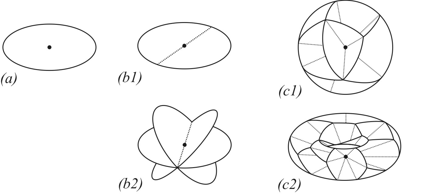
Figure 1. Examples of neighborhoods of points of a scar.  The neighborhood in (c2) is shown in a schematic way, for it is a certain subset of the conus of a torus that cannot be embedded in the three dimensional Euclidean space.

Based on the different shapes of the neighborghoods we define the $2$-components, $1$-components and $0$-components of a scar, and in fact of any bidimensional homogeneous CW complex, in the following way. We define a 2-component of a scar as a connected component of the space of points whose neighborhoods are disks. Similarly, we define a 1-component as a connected component of the space of points whose neighborhoods are built from $n$ half disks, as we showed, with $n\neq 2$. Finally, we define a 0-component as a set of the form $\left\{x\right\}$, where $x$ is a point with any other type of neighborhood.

We say then that a scar, or a bidimensional homogeneous CW complex in general, is cellular if every $i$-component is an open cell of dimension $i$. Let us notice that not every scar is cellular. Let us consider the case of a polyhedron containing a succesion of faces in which every face limits with the next one along an adge of cycle $2$. Besides, let us suppose that the last face also limits with the first one along an edge of cycle $2$, closing a loop. Let us see what happens with the scar of this polyhedron. Since all the points in the scar coming from the interior of a face, as well as all the points coming from the interior of an edge of cycle 2, have neighborhoods with the shape of a disk, it follows that this “loop” of faces gives place possibly to a $2$-component with the shape of an annulus. This example is also useful to show how the $2$-components, $1$-components, and $0$-components of a scar do not have to coincide necessarily with its faces, edges and vertices.

Now, we say that a scar, or a bidimensional homogeneous CW complex in general $S$, is simple if every point in $S$ has a regular neighborhood (in $S$) shaped like one of the three types of neighborhoods ilustrated in the following figure. Let us recall now that a spine of a closed connected 3-manifold is called special if it is a homogeneous bidimensional CW complex that is cellular and simple (see [8]).

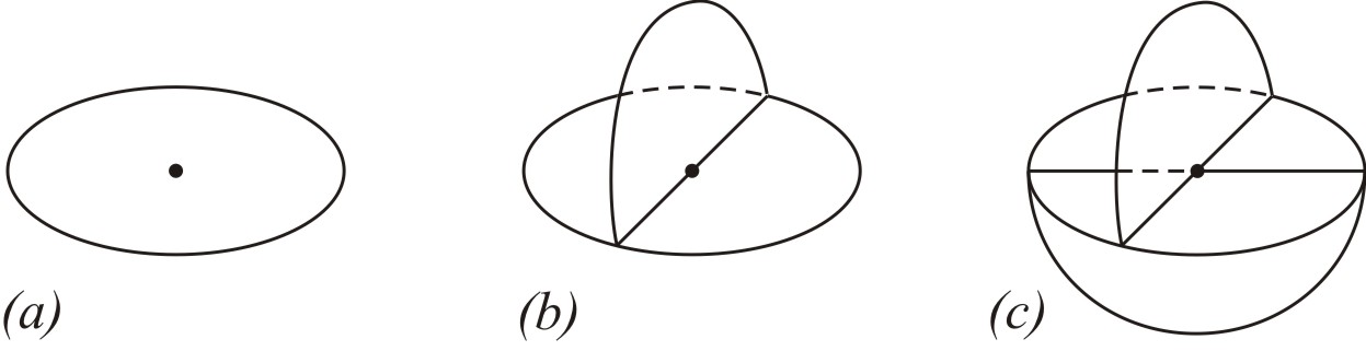
Figure 2. Neighborhoods allowed in special spines.

We shall give one more definition with the aim of simplifying the following proofs. If an edge of a scar $S$ comes from the identification of $n$ edges of cycle $n$ of the polyhedron, we say that it is an identified edge of cycle $n$. Similarly, if a vertex of $S$ comes from the identidication of $m$ vertices of order $m$ of the polyhedron, we say that it is an identified vertex of order $m$. The following four lemmas will be used to prove subsequent important results, and particulary Theorem 3.5 that is the main result of this section.

Lemma 3.1.

If a polyhedron produces a simple scar, then it produces a 3-manifold.

Proof. Let $P$ be the space produced by the polyhedron, and $S$ its scar. By Theorem 1.2 we know that every singularity of $P$, if there is any, comes from vertices of the polyhedron and therefore lies in $S$. It suffices to show then that every point of $S$ has a neighborhood in $P$ homeomorphic to a ball. For $v\in S$ let $V$ be a closed regular neighborhood of $v$ in $P$. Since $V$ is the cone of $\partial V$, to show that $V$ is a ball we only need to prove that $\partial V$ is a sphere.

We know that $V\cap S$ is a closed regular neighborhood of $v$ in $S$. Since $S$ is simple, $V\cap S$ has neccesarily one of the shapes (a), (b) o (c) shown in Figure 2. Besides, $\partial V\cap S$ is a graph embedded in $\partial V$ in such a way that $\partial V-S$ consists of open disks. For this reason, $\partial V\cap S$ induces a CW complex structure in $\partial V$. If $V\cap S$ has the shape (a), then $\partial V\cap S$ is a circumference for which $\partial V$ is neccesarily a sphere. If $V\cap S$ has the shape (b), then $\partial V\cap S$ is a graph formed by a circumference and one diameter, for which $\partial V$ is neccesarily a sphere. Finally, If $V\cap S$ has the shape (c), then $\partial V\cap S$ is a complete graph of order 4, that is, a circumference with three radii, for which, once again, $\partial V$ is a sphere. In every case the conclusion holds because none of the three graphs can be embedded in a closed, connected, orientable 2-manifold, other than the sphere, splitting it into open disks. $\square$

Lemma 3.2.

A scar is simple if and only if there exists a polyhedron that produces it satisfying the following three conditions: All of its edges are of cycle $2$ or $3$, all of its vertices are of order less than or equal to $4$, and all of its vertices are adjacent to exactly three edges of cycle $3$.

Proof. The implication from left to right follows naturally from the neighborhood analysis just exposed. Let us see the other implication. We need to show that given a polyhedron with the three properties stated, then every point of its scar has a regular neighborhood in that scar with one of the three shapes allowed. From the previous neighborhood analysis we have that the points in the faces of the scar have neighborhoods with the shape of a disk (Figure 2, (a)). We also have that, since the polyhedron has only edges of cycles 2 and 3, the points in the edges of the scar have neighborhoods homeomorphic either to a disk or to three half disks glued by its diameters (Figure 2, (a) y (b)).

It only remains then to examine the case of vertices. Let $v$ be a vertex of the scar, then $v$ is by hypotesis an identified vertex of order less than or equal to 4. However, $v$ does not have order 1 because that would imply the existence of edges of cycle 1. On the other hand, let us suppose that $v$ has order 3. Then there exist neccesarily two identified edges of cycle 3 adjacent to $v$; and $v$ has a neighborhood with the shape of three half disks, as in Figure 2. (b). But this implies that the three vertices in the polyhedron whose identification turns them into $v$ are adjacent to exactly two edges of cycle 3, which violates the hypotheses. As a consecuence, $v$ does not have order 3 either.

We conclude that $v$ has neccesarily order 2 or 4. If $v$ has order 2, then every identified edge in the scar adjacent to $v$ has order 2, and $v$ has a neighborhood with the shape of a disk.

Let us consider now the case of $v$ having order 4. Let $P$ and $S$ be respectively the space and scar produced by the polyhedron. Since $P$ is a pseudomanifold, we know that a closed neighborhood $V$ of $v$ in $P$ is homeomorphic to the cone of $\partial V$, which is a closed, connected, orientable 2-manifold. We know also that $V\cap S$ is a closed regular neighborhood of $v$ in $S$. Besides, $\partial V\cap S$ is a graph embedded in $\partial V$ in such a way that $\partial V-S$ consists of open disks, for which $\partial V\cap S$ induces a CW complex structure in $\partial V$. Now, since every vertex of the polyhedron is adjacent to exactly three edges of order 3, we see that $\partial V-S$ consists in fact of open triangles, and that the CW structure induced in $\partial V$ by $\partial V\cap S$ is a triangulation. Let us denote by $K$ the triangulation of $\partial V$ thus obtained.

Since $v$ has order 4, then $K$ has only four triangles. Besides, since every edge of the polyhedron has cycle 3, every point of $\partial V=\left|K\right|$ can lie, at most, in the boundary of three triangles. The only triangulation of a closed, connected, orientable 2-manifold, made of four triangles, and satisfying this condition, is that of the sphere triangulated as a tetrahedron. Hence, $V\cap S$ has the shape shown in Figure 2. (c). $\square$

Lemma 3.3.

A scar is cellular if and only of there exists a polyhedron that produces it not containing edges of cycle $2$.

Proof. Let $S$ be a cellular scar. Then, since every $i$-component of $S$ is an open $i$-dimensional cell, the set $C$ of $i$-components of $S$ endows $S$ with a CW complex structure, or in other words, $(S,C)$ is a CW complex.

Let us recall that in the proof of Theorem 2.1, to prove that every spine $\check{S}$ is the scar of some polyhedron, we started from the fact that $\check{S}$ had some homogeneous CW complex structure. From there we proceeded to triangulate $\check{S}$, and then to construct a polyhedron. However, let us notice that if $S$ is a simple scar, taking $S$ with the CW complex structure $(S,C)$ that we defined, we can carry out just the same construction of the proof of Theorem 2.1, but abstaining from triangulating $S$ (The $\Delta$’s appearing in the proof will not be then tetrahedra but pyramids with polygonal bases). In this way we obtain a polyhedron $\left\langle B^{3},G,\epsilon\right\rangle$ that produces $S$.

It only remains to see that $\left\langle B^{3},G,\epsilon\right\rangle$ has no edges of cycle $2$. This is true because, due to the construction of $\left\langle B^{3},G,\epsilon\right\rangle$, the $2$-components, $1$-components and $0$-components of $S$ coincide exactly with its faces, edges and vertices. The interiors of the faces of $\left\langle B^{3},G,\epsilon\right\rangle$ produce, when identified, exactly the 2-components of $S$. Similarly, the edges of $\left\langle B^{3},G,\epsilon\right\rangle$ produce exactly the 1-components of $S$, and the vertices the 0-components. This implies that no point in $S$ coming from an edge of $\left\langle B^{3},G,\epsilon\right\rangle$ has a neighborhood with the shape of a disk, and by our analysis of neighborhoods we can conclude that $\left\langle B^{3},G,\epsilon\right\rangle$ has no edges of cycle $2$.

On the other hand, it is easy to see that if a polyhedron has no edges of cycle 2, the scar produced by it is necessarily cellular. $\square$

Lemma 3.4.

Let $\left\langle B^{3},G,\epsilon\right\rangle$ be a polyhedron all whose edges are of cycle 3, all whose vertices are or order less than or equal to 4, and all whose vertices are adjacent to exactly three edges. Then every vertex of $\left\langle B^{3},G,\epsilon\right\rangle$ is of order equal to 4.

Proof. We have already proven this before unintentionally. The existence of vertices of order 1 is discarded because it implies the existence of edges of cycle 1. Besides those vertices, if they existed, would be needless. The existence of vertices of order 2 is similarily descarded because it implies the existence of edges of cycle 2. Finally, let us suppose that a vertex $v$ has order 3. Then, there necessarily exist two identified edges of cycle 3 adjacent to $v$, and $v$ has a neighborhood with the shape of three half disks, as in Figure 2. (b) But this implies that the three vertices in the polyhedron whose identification turns them into $v$ are, each of them, adjacentent to exactly two edges of cycle 3, which violates the hypotheses. We conclude then that every vertex has order 4. $\square$

We will continue with the following definition. We say that a polyhedron is distinguished if all of its edges are of cycle 3, all its vertices are of order 4, and all its vertices are adjacent to exactly three edges. It can be proved that in fact the condition of the vertices to have order 4 is superfluous, for it is implied by the other two conditions. We are in a position now to prove the following theorem, that is the main result of this section, and establishes the equivalence between the scars of distinguished polyhedra that produce 3-manifolds, and the special spines of 3-manifolds.

Theorem 3.5.

Let $M$ be a closed, connected, orientable 3-manifold, and $S\subseteq M$. Then, $S$ is a special spine of $M$ if and only if it is the scar of a distinguished polyhedron that produces $M$.

Proof. It follows from Lemmas 3.2, 3.3 and 3.4 that a scar is simple and cellular if and only if there exists a distinguished polyhedron that produces it. We will use this fact along the proof.

Let $S$ be a special spine of the manifold $M$. Let us see that there exists a distinguished polyhedron that produces $S$ and $M$. By Theorem 2.1, we know that $S$ is the scar of a polyhedron $\left\langle B^{3},H,\eta\right\rangle$ that produces $M$. However, we have no way to know wether $\left\langle B^{3},H,\eta\right\rangle$ is distinguished or not, for which this polyhedron is not of interest to us. What interest us in this regard is the fact that the spine $S$ is also a scar. This fact, in conjunction with the definition of special spine, implies that $S$ is furthermore a simple and cellular scar. Therefore, there exists a distinguished polyhedron $\left\langle B^{3},G,\epsilon\right\rangle$ that produces $S$. Let us see then that $\left\langle B^{3},G,\epsilon\right\rangle$ produces $M$ also.

Let $P$ be the space produced by $\left\langle B^{3},G,\epsilon\right\rangle$. Then, since $S$ is the scar of $\left\langle B^{3},G,\epsilon\right\rangle$ and $S$ is simple, by Lemma 3.1, $P$ is a 3-manifold. Besides, by Theorem 2.1, $S$ is a spine of $P$. Moreover, since $S$ is a special spine of $M$, by its own topology $S$ is a special spine of $P$. Now, since $S$ is a special spine of both $P$ and $M$, we have that $P=M$; given that two manifolds with homeomorphic special spines are necessarily homeomorphic (see [8]).

On the other hand, if $\left\langle B^{3},G,\epsilon\right\rangle$ is a distinguished polyhedron that produces $M$, and if $S$ is its scar, we have by Theorem 2.1 that $S$ is a spine of $M$. Moreover, since $\left\langle B^{3},G,\epsilon\right\rangle$ is distinguished, $S$ is a simple and cellular scar for which it is in fact a special spine of $M$. $\square$

4. Distinguished Polyhedra

In this section we will prove that the distinguished polyhedra are a presentation of the closed, connected, orientable 3-manifolds. This presentation is in fact equivalent to the presentation by special thickenable (PL) polyhedra, or special spines, as we will prove in Section 6 (see [8]).

Theorem 4.1.

Let $\left\langle B^{3},G,\epsilon\right\rangle$ be a distinguished polyhedron, and $S$ its scar. Then, the space produced by $\left\langle B^{3},G,\epsilon\right\rangle$ is a 3-manifold, and $S$ is a special spine of such 3-manifold.

Proof. Since $\left\langle B^{3},G,\epsilon\right\rangle$ is distinguished, $S$ is simple and, by Lemma 3.1, $\left\langle B^{3},G,\epsilon\right\rangle$ produces a 3-manifold. By Theorem 3.5, $S$ is a special spine of such 3-manifold. $\square$

Theorem 4.2.

The distinguished polyhedra are a presentation of the closed, connected, orientable 3-manifolds; where each polyhedron presents the manifold that is its quotient space.

Proof. It only remains to see that for every 3-manifold $M$ of this type there exists a distinguished polyhedron that produces it. This is true because $M$ has some special spine (see [8]), and by Theorem 3.5 that spine is the scar of a distinguished polyhedron that produces $M$. $\square$

5. Spines and Polyhedra

Up to this point we have fully established the relation between the spines of 3-manifolds and the scars of polyhedra. Our task now will be to establish a more direct relation between spines and polyhedra. Specifically, we will establish sufficient and necessary conditions for two polyhedra to produce the same quotient space and the same scar.

Let us recall for a moment the concept of alikeness between relations given in Definition 3, and consider two polyhedra $\left\langle B^{3},G,\epsilon\right\rangle$ and $\left\langle B^{3},H,\eta\right\rangle$. For $\left\langle B^{3},G,\epsilon\right\rangle$ we define $\check{E}q\epsilon$ as the relation obtained by adding to $Eq\epsilon$ every one-point set of the form $\left\{x\right\}$, with $x\in\mathring{B}$. We define $\check{E}q\eta$ in the same way. Let us notice that relations $Eq\epsilon$ and $Eq\eta$ in $\partial B^{3}$ are alike if and only if relations $\check{E}q\epsilon$ and $\check{E}q\eta$ on $B^{3}$ are alike.

Now, if $\left\langle B^{3},G,\epsilon\right\rangle$ and $\left\langle B^{3},H,\eta\right\rangle$ are polyhedra for which $Eq\epsilon$ and $Eq\eta$ are alike, we say that $\left\langle B^{3},G,\epsilon\right\rangle$ and $\left\langle B^{3},H,\eta\right\rangle$ are alike polyhedra. The following lemma is clear.

Lemma 5.1.

Alikeness between polyhedra is an equivalence relation. Besides, alike polyhedra produce the same quotient space, and the same scar.

From now on, if $Eq\epsilon$ and $Eq\eta$ are alike we will just say that $Eq\epsilon=Eq\eta$. We will see now how to obtain the set of all the polyhedra alike to a determined polyhedron $\left\langle B^{3},G,\epsilon\right\rangle$. With that purpose we will define a move that allow us to shift between alike polyhedra. Let us observe that given a polyhedron, and a pair of faces $\left\{F_{i},F_{i}^{-1}\right\}$ of such polyhedron, we can draw a line or edge $a$ that goes across $F_{i}$ from one side to another, and at the same time draw a line $a^{-1}$ in $F_{i}^{-1}$ whose points are the images of the points of $a$ under $\epsilon_{i}$, so that when $F_{i}$ and $F_{i}^{-1}$ are glued, $a$ glues with $a^{-1}$. Let us notice that this process does not alter the polyhedron substantially, and that in this case $\left\{a,a^{-1}\right\}$ is a cycle of two edges of cycle two. We call this process the insertion of an edge of cycle two, and we can conceive the remotion of an edge of cycle two in a similar way. Insertion and remotion of edges of cycle 2 will be the moves that will allow us to shift between alike polyhedra, and formally we define them in the following way. The notation “$\,:\,$” will be used for adjacency between cells.

Let $\left\langle B^{3},G,\epsilon\right\rangle$ be a polyhedron with faces $\left\{F_{1},F_{1}^{-1},...,F_{n},F_{n}^{-1}\right\}$ and identification scheme $\epsilon=\left\{\epsilon_{1},...,\epsilon_{i},\epsilon_{j},...,\epsilon_{n}\right\}$. Let $\left\{a_{1},a_{2}\right\}$ be a class of two edges of cycle 2 in $\left\langle B^{3},G,\epsilon\right\rangle$, and $F_{i}$ and $F_{j}$ be the faces of the polyhedron for which $F_{i}:a_{1}:F_{j}$ and $F_{i}^{-1}:a_{2}:F_{j}^{-1}$ holds. Let us notice that $F_{i}$ and $F_{j}$ are not necessarily different. Now, let us set $G^{\prime}=\overline{G-(\bar{a}_{1}\cup\bar{a}_{2})}$ and $\delta=\left\{\epsilon_{1},...,\epsilon_{i}\cup\epsilon_{j},...,\epsilon_{n}\right\}$. Thus, if $G^{\prime}$ is connected, then $\left\langle B^{3},G^{\prime},\delta\right\rangle$ is a polyhedron alike to $\left\langle B^{3},G,\epsilon\right\rangle$, and we say that the first one is obtained from the second one by the remotion of an edge of cycle 2.

On the other hand, let $F_{i}$ be a face of $\left\langle B^{3},G,\epsilon\right\rangle$. For $x\in F_{i}\cap G$ and $y\in F_{i}$, let $f:[0,1]\longrightarrow F_{i}$ be a continuous injective function such that $f(0)=x$ and $f(1)=y$. Let us define $a_{1}$ as $a_{1}=f([0,1])$, and $a_{2}$ as the image of $a_{1}$ under $\epsilon_{i}$. Then, depending on whether $y$ belongs or not to $G$, $F_{i}-a_{1}$ may have two connected components or only one. If $F_{i}-a_{1}$ has two connected components, we denote its closures by $F_{j}$ and $F_{k}$, with $k>j>n$. If $F_{i}-a_{1}$ has a single connected component, we will understand that $F_{j}:=F_{k}:=F_{i}$. Aditionally, we will define $F_{j}^{-1}$ and $F_{k}^{-1}$ as the images of $F_{j}$ and $F_{k}$ under $\epsilon_{i}$; and we will define $\epsilon_{j}$ and $\epsilon_{k}$ as the restrictions of $\epsilon_{i}$ to $F_{j}$ and $F_{k}$ respectively. Finally, let us set $G^{\prime}=G\cup a_{1}\cup a_{2}$, and $\delta=\left\{\epsilon_{1},...,\epsilon_{i-1},\epsilon_{i+1},...,\epsilon_{n},\epsilon_{j},\epsilon_{k}\right\}$. Then, under these circumstances, $\left\langle B^{3},G^{\prime},\delta\right\rangle$ is a polyhedron alike to $\left\langle B^{3},G,\epsilon\right\rangle$, and we say that the first one is obtained from the second one by the insertion of an edge of cycle 2.

We can state now the following lemma.

Lemma 5.2.

Two polyhedra are alike if and only if one of them can be obtained from the other by insertion and remotion of edges of cycle 2.

Proof. The implication from right to left is obtained directly from the definition of insertion and remotion of edges of cycle 2. Let us see the other implication. Let $\left\langle B^{3},G,\epsilon\right\rangle$ and $\left\langle B^{3},H,\eta\right\rangle$ be two polyhedra in the same alikeness class. Then we can consider the graph $G\cup H$ in $\partial B^{3}$. If $G\cup H$ is not connected, we can connect it by the insertion of an edge of cycle 2 and obtain a new graph $J$. If $G\cup H$ is connected, we define $J$ simply by $J=G\cup H$. Since $J$ is connected, $\left\langle B^{3},J\right\rangle$ is a cell-divided ball. Restricting the relation $Eq\epsilon=Eq\eta$ to each of the faces of $\left\langle B^{3},J\right\rangle$ we obtain relations $\delta_{1},...,\delta_{n}$, such that $\delta$ is an identification scheme for $\left\langle B^{3},J\right\rangle$. Hence, $\left\langle B^{3},J,\delta\right\rangle$ is a polyhedron in the alikeness class of $\left\langle B^{3},G,\epsilon\right\rangle$ and $\left\langle B^{3},H,\eta\right\rangle$.

Let $\Gamma$ be the set of all the points $x\in\partial B^{3}$, whose equivalence classes under $Eq\epsilon$ have cardinal different from $2$. Let us see that $\Gamma$ is contained in $G\cap H$. From the discussion of Section 3, about the shapes of the neighborhoods of the points in the scars, it follows that the points in the scar of $\left\langle B^{3},G,\epsilon\right\rangle$ coming from points in $\Gamma$ cannot have neighborhoods (on the same scar) homeomorphic to disks, and therefore $\Gamma$ must be a subset of $G$. Furthermore, that analysis reveals that $\Gamma$ is in fact a subgraph of $G$. Since $Eq\epsilon=Eq\eta$, by symmetry, $\Gamma$ must also be a subset of $H$. Thus, $\Gamma\subseteq G\cap H$.

The same argument shows that $\Gamma\subseteq G\cap J$ and that $\Gamma\subseteq H\cap J$. Since $G$ and $H$ are subgraphs of $J$, we conclude that both $\left\langle B^{3},G,\epsilon\right\rangle$ and $\left\langle B^{3},H,\eta\right\rangle$ can be obtained from $\left\langle B^{3},J,\delta\right\rangle$ by the remotion of edges of cycle 2, with which we have proven the lemma. $\square$

Let $P$ be a pseudomanifold of type $\mathcal{P}_{1}o$, and let $S$ be an homogeneous bidimensional spine of $P$. Then we say that a polyhedron produces $(P,S)$ if the space that it produces is $P$ and its scar is $S$. We are in a position now to prove the following theorem, that will be the main result of this section, and establishes the equivalence between the pairs of the form $(P,S)$ and the alikeness classes of polyhedra.

Theorem 5.3.

Two polyhedra are alike if and only of they produce the same quotient space and the same scar.

Proof. We already know that alike polyhedra produce the same space and the same scar (Lemma 5.1). Let us see now that if two polyhedra produce the same quotient space $P$, and the same scar $S$, then they are alike.

The proof is based on the construction made in the proof of Theorem 2.1, to prove that every spine is the scar of some polyhedron. Let us observe that given a triangulation $T$ of $S$, the construction of such polyhedron, just as it was carried out in the proof of the theorem, leads to a unique polyhedron; for which we can denote the same by $\left\langle B^{3},G_{T},\epsilon_{T}\right\rangle$. Let us see first that the polyhedra obtained from $P$ and $S$ by this method starting from different triangulations are all alike. Let us consider two triangulations $K$ and $L$ of $S$, and let us take one more triangulation, $R$, that be a common subdivision of $K$ and $L$. Then $\left\langle B^{3},G_{R},\epsilon_{R}\right\rangle$ can be obtained from both $\left\langle B^{3},G_{K},\epsilon_{K}\right\rangle$ and $\left\langle B^{3},G_{L},\epsilon_{L}\right\rangle$ by insertion of edges of cycle 2, for which $\left\langle B^{3},G_{K},\epsilon_{K}\right\rangle$ and $\left\langle B^{3},G_{L},\epsilon_{L}\right\rangle$ are alike.

Now, let $\left\langle B^{3},H,\eta\right\rangle$ be an arbitrary polyhedron that produces $M$ and $S$. Let us see that there exists a triangulation $T$ of $S$ for which $\left\langle B^{3},H,\eta\right\rangle$ and $\left\langle B^{3},G_{T},\epsilon_{T}\right\rangle$ are alike. Through the insertion of edges of cycle 2 in $\left\langle B^{3},H,\eta\right\rangle$, it is possible to obtain a polyhedron $\left\langle B^{3},H^{\prime},\eta^{\prime}\right\rangle$ whose faces are all triangular. Clearly $H^{\prime}$ induces a triangulation $T_{0}$ in $S$, and it is easy to see that $\left\langle B^{3},H^{\prime},\eta^{\prime}\right\rangle=\left\langle B^{3},G_{T_{0}},\epsilon_{T_{0}}\right\rangle$. Thus, $T_{0}$ is a triangulation of $S$ such that $\left\langle B^{3},G_{T_{0}},\epsilon_{T_{0}}\right\rangle$ and $\left\langle B^{3},H,\eta\right\rangle$ are alike.

In this way we have that if $T$ is a triangulation of $S$, every polyhedron that produces $M$ and $S$ is alike to $\left\langle B^{3},G_{T},\epsilon_{T}\right\rangle$, which completes the proof. $\square$

The following theorem establishes the equivalence between the pairs of the form $(M,S)$ (where $M$ is a closed, connected, orientable 3-manifold, and $S$ is a homogeneous bidimensional spine of $M$) and the alikeness classes of polyhedra that produce manifolds.

Theorem 5.4.

Let $M$ be a closed, connected, orientable 3-manifold, and suppose that $S$ is a homogeneous bidimensional spine of $M$. Then, there exists a unique alikeness class, such that all its polyhedra produce $(M,S)$, and such that no other polyhedron produces $(M,S)$.

Proof. It follows trivially from Theorems 2.1 and 5.3. $\square$

6. Special Spines and Polyhedra

In Section 3 we established the relation between the special spines of 3-manifolds and the scars of distinguished polyhedra. In this last section, in light of the developments of the previous section, we will aim for a more direct relation between special spines and distinguished polyhedra. This will be acomplished in the main result of this section, which is given in Theorem 6.3, and establishes the equivalence between the distinguished polyhedra and the special spines of 3-manifolds (or special thickenable PL polyhedra).

Before stating this result we shall give some definitions. Let $\left\langle B^{3},G,\epsilon\right\rangle$ be a polyhedron, and let $\Gamma$ be definied as in the proof of Lemma 5.2, that is, as the set of all points $x\in\partial B^{3}$, whose equivalence classes under $Eq\epsilon$ have cardinal different from $2$. Then $\Gamma$ is a subgraph of $G$, as we saw in that proof. Since $\Gamma$ is defined from $Eq\epsilon$ and not from $\left\langle B^{3},G,\epsilon\right\rangle$, we see that $\Gamma$ only depends on the alikeness class of $\left\langle B^{3},G,\epsilon\right\rangle$. We call $\Gamma$ the essential graph of the class of $\left\langle B^{3},G,\epsilon\right\rangle$.

Let us notice that $\Gamma$ does not necessarily have to be connected or non-empty, though it can be proven that it is empty only in the case of a certain polyhedron for the projective space. Let us observe that if $\Gamma$ is connected and non-empty, $\left\langle B^{3},\Gamma\right\rangle$ is by definition a cell-divided ball. Moreover, the restrictions of $Eq\epsilon$ to each of the faces of $\left\langle B^{3},\Gamma\right\rangle$ produce an identification scheme $\gamma$ for $\left\langle B^{3},\Gamma\right\rangle$, such that $Eq\gamma=Eq\epsilon$. Thus, if $\Gamma$ is connected and non-empty, $\left\langle B^{3},\Gamma,\gamma\right\rangle$ is a well defined polyhedron. We call $\left\langle B^{3},\Gamma,\gamma\right\rangle$ the minimum polyhedron of the class of $\left\langle B^{3},G,\epsilon\right\rangle$.

Now, let $\Gamma$ be the essential graph (connected and non-empty) of some alikeness class $A$, and let $\left\langle B^{3},G,\epsilon\right\rangle$ be a class representative for $A$. Then, the analysis of neighborhoods of Section 3 reveals that $\Gamma$, besides being a subgraph of $G$, is the union of the closures of all the edges of $G$ with cycle different from 2. Hence, $\left\langle B^{3},\Gamma,\gamma\right\rangle$ is the polyhedron obtained by succesively removing all the edges of cycle 2 from $\left\langle B^{3},G,\epsilon\right\rangle$. The arbitrariness of $\left\langle B^{3},G,\epsilon\right\rangle$ implies that we have proven the following lemma.

Lemma 6.1.

If $\left\langle B^{3},\Gamma,\gamma\right\rangle$ is the minimum polyhedron of an alikeness class $A$, with $\Gamma$ connected and non-empty, then every polyhedron in $A$ is obtained from $\left\langle B^{3},\Gamma,\gamma\right\rangle$ by the insertion of edges of cycle 2.

We can prove now the following theorem.

Theorem 6.2.

Every distinguished polyhedron produces a closed, connected, orientable 3-manifold, and its scar is a special spine of that manifold. Inversely, if $M$ is a closed, connected, orientable 3-manifold and $S$ is a special spine of $M$, then there exists a unique distinguished polyhedron that produces $M$ and whose scar is $S$.

Proof. The first statement is almost exactly the statement of Theorem 4.1. The closedness, connectedness and orientability are implied by Theorem 1.2. Let us prove now the other affirmation. Let $M$ be a (closed, connected, orientable) 3-manifold and $S$ a special spine of $M$. Then we have by Theorem 3.5 that there exists a distinguished polyhedron $\left\langle B^{3},G,\epsilon\right\rangle$ that produces $(M,S)$. On the other hand we have, by Theorem 5.4, that there exists a unique alikeness class $A$ whose polyhedra produce $(M,S)$. From there it follows that $\left\langle B^{3},G,\epsilon\right\rangle$ belongs to $A$.

The theorem will be proven if we show that $\left\langle B^{3},G,\epsilon\right\rangle$ is the only distinguished polyhedron in $A$. Now, we know that $\left\langle B^{3},G,\epsilon\right\rangle$, for being distinguished, lacks edges of cycle 2. Since the essential graph of $A$ is the union of the closures of all the edges of $G$ with cycle different from 2, we have that $G$ is the essential graph of $A$. Hence, since $\left\langle B^{3},G,\epsilon\right\rangle$ is a well defined polyhedron, $G$ is connected and non-empty, and $\left\langle B^{3},G,\epsilon\right\rangle$ is the minimum polyhedron of $A$. From there it follows that every polyhedron in $A$ is obtained from $\left\langle B^{3},G,\epsilon\right\rangle$ by the insertion of edges of cycle 2 (Lemma 6.1), and that $\left\langle B^{3},G,\epsilon\right\rangle$ is the only distinguished polyhedron in $A$. $\square$

Theorem 6.3.

Every distinguished polyhedron has as its scar a special spine. Inversely, for every special spine there exists a unique distinguished polyhedron that has it as its scar.

Proof. The first affirmation holds by Theorem 4.1. Let us see the other affirmation. Let $S$ be a special spine of some closed, connected, orientable 3-manifold. Since $S$ is special, that 3-manifold is unique, and we can denote it by $M_{S}$. By the previous theorem (Theorem 6.2), there exists a unique distinguished polyhedron that produces $(M_{S},S)$. From there it follows that there exists a unique distinguished polyhedron that produces $S$. $\square$

The previous theorem, which is the main result of this section, establishes a one to one correspondence between the distinguished polyhedra and the special spines, in which each polyhedron produces its corresponding spine. It is a consecuence of the same theorem and Theorem 3.5 that, for every distinguished polyhedron, it and its corresponding special spine present one and the same 3-manifold. We conclude then that the presentations of 3-manifolds by distinguished polyhedra and special spines are in fact equivalent.

References

- [1] J. W. Cannon, W. J. Floyd and W. R. Parry, Introduction to Twisted Face-Pairings. Math. Res. Lett. 7 (2000), 477-491.
- [2] J. W. Cannon, W. J. Floyd and W. R. Parry, Twisted Face-Pairing 3-Manifolds. Trans. Amer. Math. Soc. 354 (2002), 2369-2397.
- [3] J. W. Cannon, W. J. Floyd and W. R. Parry, Heegaard Diagrams and Surgery Descriptions for Twisted Face-Pairing 3-Manifolds. Algebr. Geom. Topol. 3 (2003), 235-285.
- [4] M. H. Hilden, J. M. Montesinos, D. M. Tejada y M. M. Toro, A New Representation of Links: Butterflies. Preprint.
- [5] M. H. Hilden, M. T. Lozano, J. M. Montesinos, On a Remarkable Polyhedron Geometrizing the Figure Eight Knot Cone Manifolds. J. Math. Sci. Univ. Tokyo 2 (1995), 501–561.
- [6] P. S. Isaza, Modificaciones en Poliedros con Caras Identificadas. Magister Thesis, Universidad Nacional de Colombia, Medellín, 2011.
- [7] S. Matveev, Complexity Theory of Three-Dimensional Manifolds. Acta Appl. Math. 19 (1990) 101–130.
- [8] S. Matveev, Algorithmic Topology and Classification of 3-Manifolds. Springer-Verlag, Berlin, 2007.
- [9] S. Matveev, M. A. Ovchinnikov and M. V. Sokolov, Construction and Properties of the -Invariant. J. Math. Sci. 113 (2003), 849-855.
- [10] S. Matveev, D. Rolfsen. Spines and Embeddings of -Manifolds. J. London Math. Soc. 59 (1999), no. 1, 359–368.
- [11] B. Martelli, C. Petronio. Complexity of Geometric Three-Manifolds. Geom. Dedicata 108 (2004) 15-69.
- [12] J. M. Montesinos, Sobre la Conjetura de Poincaré y los Recubridores Ramificados sobre un Nudo. Doctoral Thesis, Published by the Department of Publications of the Faculty of Sciences of the Universidad Complutense of Madrid, 1971.
- [13] J. M. Montesinos, Reducción de la Conjetura de Poincaré a otras Conjeturas Geométricas. Rev. Mat. Hisp. Amer. 32 (1972), 33-51.
- [14] J. M. Montesinos, Classical Tessellations and Three-Manifolds. Springer-Verlag, New York, 1987.
- [15] D. Rolfsen, Knots and Links, Publish or Perish, Inc., Berkeley, CA, 1976.
- [16] H. Seifert, y W. Threlfall, Lehrbuch der Topologie. Teubner, Leipzig, 1934.
- [17] M. M. Toro, Enlaces de tres Puentes y Mariposas. Universidad Nacional de Colombia, Medellín, 2010.