Weak Galerkin Finite Element Methods on Polytopal Meshes

Abstract

This paper introduces a new weak Galerkin (WG) finite element method for second order elliptic equations on polytopal meshes. This method, called WG-FEM, is designed by using a discrete weak gradient operator applied to discontinuous piecewise polynomials on finite element partitions of arbitrary polytopes with certain shape regularity. The paper explains how the numerical schemes are designed and why they provide reliable numerical approximations for the underlying partial differential equations. In particular, optimal order error estimates are established for the corresponding WG-FEM approximations in both a discrete $H^{1}$ norm and the standard $L^{2}$ norm. Numerical results are presented to demonstrate the robustness, reliability, and accuracy of the WG-FEM. All the results are derived for finite element partitions with polytopes. Allowing the use of discontinuous approximating functions on arbitrary polytopal elements is a highly demanded feature for numerical algorithms in scientific computing.

1 Introduction

In this paper, we are concerned with a further and new development of weak Galerkin (WG) finite element methods for partial differential equations. Our model problem is a second-order elliptic equation which seeks an unknown function $u=u(x)$ satisfying

(1) $$-\nabla\cdot(a(x,u,\nabla u)\nabla u)=f(x),\quad\mbox{in}\ \Omega,$$

where $\Omega$ is a polytopal domain in $\mathbb{R}^{d}$ (polygonal or polyhedral domain for $d=2,3$), $\nabla u$ denotes the gradient of the function $u=u(x)$, and $a=a(x,u,\nabla u)$ is a symmetric $d\times d$ matrix-valued function in $\Omega$. We shall assume that the differential operator is strictly elliptic in $\Omega$; that is, there exists a positive number $\lambda>0$ such that

(2) $$\xi^{t}a(x,\eta,p)\xi\geq\lambda\xi^{t}\xi,\qquad\forall\xi\in\mathbb{R}^{d},$$

for all $x\in\Omega,\eta\in\mathbb{R},p\in\mathbb{R}^{d}$. Here $\xi$ is understood as a column vector and $\xi^{t}$ is the transpose of $\xi$. We also assume that the differential operator has bounded coefficients; that is for some constant $\Lambda$ we have

(3) $$|a(x,\eta,p)|\leq\Lambda,$$

for all $x\in\Omega,\eta\in\mathbb{R},$ and $p\in\mathbb{R}^{d}$.

Introduce the following form

(4) $$\mathfrak{a}(\phi;u,v):=\int_{\Omega}a(x,\phi,\nabla\phi)\nabla u\cdot\nabla vdx.$$

For simplicity, let the function $f$ in (1) be locally integrable in $\Omega$. We shall consider solutions of (1) with a non-homogeneous Dirichlet boundary condition

(5) $$u=g,\quad\mbox{on}\ \partial\Omega,$$

where $g\in H^{\frac{1}{2}}(\partial\Omega)$ is a function defined on the boundary of $\Omega$. Here $H^{1}(\Omega)$ is the Sobolev space consisting of functions which, together with their gradients, are square integrable over $\Omega$. $H^{\frac{1}{2}}(\partial\Omega)$ is the trace of $H^{1}(\Omega)$ on the boundary of $\Omega$. The corresponding weak form seeks $u\in H^{1}(\Omega)$ such that $u=g$ on $\partial\Omega$ and

(6) $$\mathfrak{a}(u;u,v)=F(v),\qquad\forall v\in H_{0}^{1}(\Omega),$$

where $F(v)\equiv\int_{\Omega}fvdx$.

Galerkin finite element methods for (6) refer to numerical techniques that seek approximate solutions from a finite dimensional space $V_{h}$ consisting of piecewise polynomials on a prescribed finite element partition ${\mathcal{T}}_{h}$. The method is called conforming if $V_{h}$ is a subspace of $H^{1}(\Omega)$. Conforming finite element methods are then formulated by solving $u_{h}\in V_{h}$ such that $u_{h}=I_{h}g$ on $\partial\Omega$ and

(7) $$\mathfrak{a}(u_{h};u_{h},v)=F(v),\qquad\forall v\in V_{h}\cap H_{0}^{1}(\Omega),$$

where $I_{h}g$ is a certain approximation of the Dirichlet boundary value. When $V_{h}$ is not a subspace of $H^{1}(\Omega)$, the form $\mathfrak{a}(\phi;u,v)$ is no longer meaningful since the gradient operator is not well-defined for non-$H^{1}$ functions in the classical sense. Nonconforming finite element methods arrive when the gradients in $\mathfrak{a}(\phi;u,v)$ are taken locally on each element where the finite element functions are polynomials. More precisely, the form $\mathfrak{a}(\phi;u,v)$ in nonconforming finite element methods is given element-by-element as follows

(8) $$\mathfrak{a}_{h}(\phi;u,v):=\sum_{T\in{\mathcal{T}}_{h}}\int_{T}a(x,\phi,\nabla\phi)\nabla u\cdot\nabla vdx.$$

When $V_{h}$ is close to be conforming, the form $\mathfrak{a}_{h}(\phi;u,v)$ shall be an acceptable approximation to the original form $\mathfrak{a}(\phi;u,v)$. The key in the nonconforming method is to explore the maximum non-conformity of $V_{h}$ when the approximate form $\mathfrak{a}_{h}(\phi;u,v)$ is required to be sufficiently close to the original form.

A natural generalization of the nonconforming finite element method would occur when the following extended form of (8) is employed

(9) $$\mathfrak{a}_{w}(\phi;u,v):=\sum_{T\in{\mathcal{T}}_{h}}\int_{T}a(x,\phi,\nabla_{w}\phi)\nabla_{w}u\cdot\nabla_{w}vdx,$$

where $\nabla_{w}$ is an approximation of $\nabla$ locally on each element. By viewing $\nabla_{w}$ as a weakly defined gradient operator, the form $\mathfrak{a}_{w}(\phi;u,v)$ would give a new class of numerical methods called weak Galerkin (WG) finite element methods.

In general, weak Galerkin refers to finite element techniques for partial differential equations in which differential operators (e.g., gradient, divergence, curl, Laplacian) are approximated by weak forms as distributions. In [17], a WG method was introduced and analyzed for second order elliptic equations based on a discrete weak gradient arising from local RT [16] or BDM [9] elements. Due to the use of the RT and BDM elements, the WG finite element formulation of [17] was limited to classical finite element partitions of triangles ($d=2$) or tetrahedra ($d=3$). In [18], a weak Galerkin finite element method was developed for the second order elliptic equation in the mixed form. The use of a stabilization for the flux variable in the mixed formulation is the key to the WG mixed finite element method of [18]. The resulting WG mixed finite element schemes turned out to be applicable for general finite element partitions consisting of shape regular polytopes (e.g., polygons in 2D and polyhedra in 3D), and the stabilization idea opened a new door for weak Galerkin methods.

The goal of this paper is to apply the stabilization idea to the form $\mathfrak{a}_{w}(\phi;u,v)$, and thus to develop a new weak Galerkin method for (1)-(5) in the primary variable $u$ that shall admit general finite element partitions consisting of arbitrary polytopal elements. The resulting WG method will no longer be limited to RT and BDM elements in the computation of the discrete weak gradient $\nabla_{w}$. In practice, allowing arbitrary shape in finite element partition provides a convenient flexibility in both numerical approximation and mesh generation, especially in regions where the domain geometry is complex. Such a flexibility is also very much appreciated in adaptive mesh refinement methods.

The main contribution of this paper is three fold: (1) the WG finite element method to be described in section 4 allows finite element partitions of arbitrary polytopes which are shape regular in the sense as defined in [18], (2) the finite element spaces constitute regular polynomial spaces on each element/face which are computation-friendly, and (3) the WG finite element scheme retains the mass conservation property of the original system locally on each element.

One close relative of the WG finite element method of this paper is the hybridizable discontinuous Galerkin (HDG) method [12]. In fact, it can be proved that our weak Galerkin method is identical to HDG method for the Poisson equation. However, the WG method differs from HDG for the model problem (1) with nonconstant coefficient matrix $a$ and more sophisticated problems. These two methods are fundamentally different in concept and formulation. The key element of HDG is the flux variable, while the key element for WG is the gradient operator through weak derivatives. For either nonlinear or degenerate coefficient matrix $a=a(x,u,\nabla u)$, the WG finite element method has obvious advantage over HDG since $\nabla u$ is approximated by $\nabla_{w}u$ and there is no need to invert the matrix $a$ in WG formulations. More importantly, the concept of weak derivatives makes WG a widely applicable numerical technique for a large variety of partial differential equations which we shall report in forthcoming papers.

The paper is organized as follows. In section 2, we introduce some standard notations in Sobolev spaces. In section 3, we review the definition and approximation of the weak gradient operator. In section 4, we provide a detailed description for the new WG finite element scheme, including a discussion on the element shape regularity assumption. In section 5, we define some local projection operators and then derive some approximation properties which are useful in error analysis. In section 6, we show that the WG finite element method retains the mass conservation property of the original system locally on each element. In section 7, we show that the weak Galerkin finite element scheme for the nonlinear problem has at least one solution. The solution existence is based on the Leray-Schauder fixed point theorem. In section 8, we shall establish an optimal order error estimate for the WG finite element approximation in a $H^{1}$-equivalent discrete norm for the linear case of (1). We shall also derive an optimal order error estimate in the $L^{2}$ norm by using a duality argument as was commonly employed in the standard Galerkin finite element methods [11, 5]. Finally in section 9, we present some numerical results which confirm the theory developed in earlier sections.

2 Preliminaries and Notations

Let $D$ be any domain in $\mathbb{R}^{d},d=2,3$. We use the standard definition for the Sobolev space $H^{s}(D)$ and their associated inner products $(\cdot,\cdot)_{s,D}$, norms $\|\cdot\|_{s,D}$, and seminorms $|\cdot|_{s,D}$ for any $s\geq 0$. For example, for any integer $s\geq 0$, the seminorm $|\cdot|_{s,D}$ is given by

$$|v|_{s,D}=\left(\sum_{|\alpha|=s}\int_{D}|\partial^{\alpha}v|^{2}dD\right)^{\frac{1}{2}}$$

with the usual notation

$$\alpha=(\alpha_{1},\dotsc,\alpha_{d}),\quad|\alpha|=\alpha_{1}+\dotsc+\alpha_{d},\quad\partial^{\alpha}=\prod_{j=1}^{d}\partial_{x_{j}}^{\alpha_{j}}.$$

The Sobolev norm $\|\cdot\|_{m,D}$ is given by

$$\|v\|_{m,D}=\left(\sum_{j=0}^{m}|v|^{2}_{j,D}\right)^{\frac{1}{2}}.$$

The space $H^{0}(D)$ coincides with $L^{2}(D)$, for which the norm and the inner product are denoted by $\|\cdot\|_{D}$ and $(\cdot,\cdot)_{D}$, respectively. When $D=\Omega$, we shall drop the subscript $D$ in the norm and inner product notation.

The space $H({\rm div};D)$ is defined as the set of vector-valued functions on $D$ which, together with their divergence, are square integrable; i.e.,

$$H({\rm div};D)=\left\{{\bf v}:\ {\bf v}\in[L^{2}(D)]^{d},\nabla\cdot{\bf v}\in L^{2}(D)\right\}.$$

The norm in $H({\rm div};D)$ is defined by

$$\|{\bf v}\|_{H({\rm div};D)}=\left(\|{\bf v}\|_{D}^{2}+\|\nabla\cdot{\bf v}\|_{D}^{2}\right)^{\frac{1}{2}}.$$

3 Weak Gradient

The key in weak Galerkin methods is the use of discrete weak derivatives in the place of strong derivatives in the variational form for the underlying partial differential equations. For the model problem (6), the gradient $\nabla$ is the principle differential operator involved in the variational formulation. Thus, it is critical to define and understand discrete weak gradients for the corresponding numerical methods. Following the idea originated in [17], the discrete weak gradient is given by approximating the weak gradient operator with piecewise polynomial functions; details are presented in the rest of this section.

Let $K$ be any polytopal domain with boundary $\partial K$. A weak function on the region $K$ refers to a function $v=\{v_{0},v_{b}\}$ such that $v_{0}\in L^{2}(K)$ and $v_{b}\in H^{\frac{1}{2}}(\partial K)$. The first component $v_{0}$ can be understood as the value of $v$ in $K$, and the second component $v_{b}$ represents $v$ on the boundary of $K$. Note that $v_{b}$ may not necessarily be related to the trace of $v_{0}$ on $\partial K$ should a trace be well-defined. Denote by $W(K)$ the space of weak functions on $K$; i.e.,

(10) $$W(K):=\{v=\{v_{0},v_{b}\}:\ v_{0}\in L^{2}(K),\;v_{b}\in H^{\frac{1}{2}}(\partial K)\}.$$

The weak gradient operator, as was introduced in [17], is defined as follows.

Definition 3.1.

The dual of $L^{2}(K)$ can be identified with itself by using the standard $L^{2}$ inner product as the action of linear functionals. With a similar interpretation, for any $v\in W(K)$, the weak gradient of $v$ is defined as a linear functional $\nabla_{w}v$ in the dual space of $H(div,K)$ whose action on each $q\in H(div,K)$ is given by

(11) $$(\nabla_{w}v,q)_{K}:=-(v_{0},\nabla\cdot q)_{K}+\langle v_{b},q\cdot{\bf n}\rangle_{\partial K},$$

where ${\bf n}$ is the outward normal direction to $\partial K$, $(v_{0},\nabla\cdot q)_{K}=\int_{K}v_{0}(\nabla\cdot q)dK$ is the action of $v_{0}$ on $\nabla\cdot q$, and $\langle v_{b},q\cdot{\bf n}\rangle_{\partial K}$ is the action of $q\cdot{\bf n}$ on $v_{b}\in H^{\frac{1}{2}}(\partial K)$.

The Sobolev space $H^{1}(K)$ can be embedded into the space $W(K)$ by an inclusion map $i_{W}:\ H^{1}(K)\to W(K)$ defined as follows

$$i_{W}(\phi)=\{\phi|_{K},\phi|_{\partial K}\},\qquad\phi\in H^{1}(K).$$

With the help of the inclusion map $i_{W}$, the Sobolev space $H^{1}(K)$ can be viewed as a subspace of $W(K)$ by identifying each $\phi\in H^{1}(K)$ with $i_{W}(\phi)$. Analogously, a weak function $v=\{v_{0},v_{b}\}\in W(K)$ is said to be in $H^{1}(K)$ if it can be identified with a function $\phi\in H^{1}(K)$ through the above inclusion map. It is not hard to see that the weak gradient is identical with the strong gradient (i.e., $\nabla_{w}v=\nabla v$) for smooth functions $v\in H^{1}(K)$.

Recall that the discrete weak gradient operator was defined by approximating $\nabla_{w}$ in a polynomial subspace of the dual of $H(div,K)$. More precisely, for any non-negative integer $r\geq 0$, denote by $P_{r}(K)$ the set of polynomials on $K$ with degree no more than $r$. The discrete weak gradient operator, denoted by $\nabla_{w,r,K}$, is defined as the unique polynomial $(\nabla_{w,r,K}v)\in[P_{r}(K)]^{d}$ satisfying the following equation

(12) $$(\nabla_{w,r,K}v,q)_{K}=-(v_{0},\nabla\cdot q)_{K}+\langle v_{b},q\cdot{\bf n}\rangle_{\partial K},\qquad\forall q\in[P_{r}(K)]^{d}.$$

The discrete weak gradient operator, namely $\nabla_{w,r,K}$ as defined in (12), was first introduced in [17] where two examples of the polynomial subspace $[P_{r}(K)]^{d}$ were thoroughly discussed and employed for the second order elliptic problem (1)-(5). The two examples make use of the Raviat-Thomas [16] and Brezzi-Douglas-Marini [9] elements developed in the classical mixed finite element method. As a result, the corresponding WG finite element method of [17] is closely related to the mixed finite element method. In this paper, we shall allow a greater flexibility in the definition and computation of the discrete weak gradient operator $\nabla_{w,r,K}$ by using the usual polynomial space $[P_{r}(K)]^{d}$. This will result in a new class of WG finite element schemes with remarkable properties to be detailed in forth coming sections.

4 Weak Galerkin Finite Element Schemes

In finite element methods, mesh generation is a crucial first step in the algorithm design. For the usual finite element methods [11, 7], the meshes are mostly required to be simplices: triangles or quadrilaterals in two dimensions and tetrahedra or hexahedra in three dimensions, or their variations known as isoparametric elements. Our new weak Galerkin finite element method is designed to be sufficiently flexible so that general meshes of polytopes (e.g., polygons in 2D and polyhedra in 3D) are allowed. For simplicity, we shall refer the elements as polygons or polyhedra in the rest of the paper.

4.1 Domain Partition

Let ${\cal T}_{h}$ be a partition of the domain $\Omega$ consisting of polygons in two dimensions or polyhedra in three dimensions satisfying a set of conditions to be specified. Denote by ${\cal E}_{h}$ the set of all edges or flat faces in ${\cal T}_{h}$, and let ${\cal E}_{h}^{0}={\cal E}_{h}\backslash\partial\Omega$ be the set of all interior edges or flat faces. For every element $T\in{\mathcal{T}}_{h}$, we denote by $|T|$ the area or volume of $T$ and by $h_{T}$ its diameter. Similarly, we denote by $|e|$ the length or area of $e$ and by $h_{e}$ the diameter of edge or flat face $e\in{\mathcal{E}}_{h}$. We also set as usual the mesh size of ${\mathcal{T}}_{h}$ by

$$h=\max_{T\in{\mathcal{T}}_{h}}h_{T}.$$

All the elements of ${\mathcal{T}}_{h}$ are assumed to be closed and simply connected polygons or polyhedra. We need some shape regularity for the partition ${\mathcal{T}}_{h}$ described as follows (see [18] for more details).

A1:

Assume that there exist two positive constants $\varrho_{v}$ and $\varrho_{e}$ such that for every element $T\in{\mathcal{T}}_{h}$ we have

(13) $$\varrho_{v}h_{T}^{d}\leq|T|,\qquad\varrho_{e}h_{e}^{d-1}\leq|e|$$

for all edges or flat faces $e$ of $T$.

A2:

Assume that there exists a positive constant $\kappa$ such that for every element $T\in{\mathcal{T}}_{h}$ we have

(14) $$\kappa h_{T}\leq h_{e}$$

for all edges or flat faces $e$ of $T$.

A3:

Assume that the mesh edges or faces are flat. We further assume that for every $T\in{\mathcal{T}}_{h}$, and for every edge/face $e\in\partial T$, there exists a pyramid $P(e,T,A_{e})$ contained in $T$ such that its base is identical with $e$, its apex is $A_{e}\in T$, and its height is proportional to $h_{T}$ with a proportionality constant $\sigma_{e}$ bounded from below by a fixed positive number $\sigma^{*}$. In other words, the height of the pyramid is given by $\sigma_{e}h_{T}$ such that $\sigma_{e}\geq\sigma^{*}>0$. The pyramid is also assumed to stand up above the base $e$ in the sense that the angle between the vector ${\bf x}_{e}-A_{e}$, for any ${\bf x}_{e}\in e$, and the outward normal direction of $e$ is strictly acute by falling into an interval $[0,\theta_{0}]$ with $\theta_{0}<\frac{\pi}{2}$.

A4:

Assume that each $T\in{\mathcal{T}}_{h}$ has a circumscribed simplex $S(T)$ that is shape regular and has a diameter $h_{S(T)}$ proportional to the diameter of $T$; i.e., $h_{S(T)}\leq\gamma_{*}h_{T}$ with a constant $\gamma_{*}$ independent of $T$. Furthermore, assume that each circumscribed simplex $S(T)$ intersects with only a fixed and small number of such simplices for all other elements $T\in{\mathcal{T}}_{h}$.

Figure 1 is a depiction of a shape-regular polygonal element in 2D. As to the property A3, for edge $e=AF$, the corresponding pyramid is given by the triangle $AA_{e}F$ which is of a similar size as the polygonal element. ${\bf n}_{e}$ is the outward normal direction to the edge $e$. The angle between the two vectors ${\bf n}_{e}$ and $\overrightarrow{A_{e}{\bf x}_{e}}$ is strictly acute for any ${\bf x}_{e}\in e$.

Fig. 1: Depiction of a shape-regular polygonal element $ABCDEFA$.

4.2 WG Finite Element Algorithms

Let ${\cal T}_{h}$ be a finite element partition that is shape regular; namely, satisfying the properties A1-A4. On each element $T\in{\mathcal{T}}_{h}$, we have a space of weak functions W(T) defined as in Section 3. Denote by $V$ the weak function space on ${\mathcal{T}}_{h}$ given by

(15) $$V:=\{v=\{v_{0},v_{b}\}:\ \{v_{0},v_{b}\}|_{T}\in W(T),T\in{\mathcal{T}}_{h}\},$$

where $\{v_{0},v_{b}\}|_{T}:=\{(v_{0})|_{T},(v_{b})|_{\partial T}\}$ is the restriction of $v$ on the element $T$.

For any given integer $k\geq 1$, let $W_{k}(T)$ be the discrete weak function space consisting of polynomials of degree $k$ in $T$ and piecewise polynomials of degree $k$ on $\partial T$; i.e.,

(16) $$W_{k}(T):=\{v=\{v_{0},v_{b}\}:\;{v_{0}}|_{T}\in P_{k}(T),\ v_{b}|_{e}\in P_{k}(e),\ e\in\partial T\}.$$

Furthermore, let $V_{h}$ be the weak Galerkin finite element space defined as follows

(17) $$V_{h}:=\{v=\{v_{0},v_{b}\}:\;\{v_{0},v_{b}\}|_{T}\in W_{k}(T),\ T\in{\mathcal{T}}_{h}\}$$

and

(18) $$V^{0}_{h}:=\{v:\ v\in V_{h},\ v_{b}=0\mbox{ on }\partial\Omega\}.$$

Denote by $\nabla_{w,k-1}$ the discrete weak gradient operator on the finite element space $V_{h}$ computed by using (12) on each element $T$; i.e.,

$$(\nabla_{w,k-1}v)|_{T}=\nabla_{w,k-1,T}(v|_{T}),\qquad\forall v\in V_{h}.$$

For simplicity of notation, from now on we shall drop the subscript $k-1$ in the notation $\nabla_{w,k-1}$ for the discrete weak gradient.

Now we introduce two forms on $V_{h}$ as follows:

$$\mathfrak{a}(\phi;v,\;w) = \sum_{T\in{\cal T}_{h}}\int_{T}a(x,\phi,\nabla_{w}\phi)\nabla_{w}v\cdot\nabla_{w}wdT,$$

$$s(v,\;w) = \rho\sum_{T\in{\cal T}_{h}}h_{T}^{-1}\langle v_{0}-v_{b},\;\;w_{0}-w_{b}\rangle_{\partial T},$$

where $\rho>0$ is a parameter with constant value. In practical computation, one might set $\rho=1$. Denote by $\mathfrak{a}_{s}(\cdot;\cdot,\;\cdot)$ a stabilization of $\mathfrak{a}(\cdot;\cdot,\;\cdot)$ given by

$$\mathfrak{a}_{s}(\phi;v,\;w):=\mathfrak{a}(\phi;v,\;w)+s(v,\;w).$$

Weak Galerkin Algorithm 1.

A numerical approximation for (1) and (5) can be obtained by seeking $u_{h}=\{u_{0},\;u_{b}\}\in V_{h}$ satisfying both $u_{b}=Q_{b}g$ on $\partial\Omega$ and the following equation:

(19) $$\mathfrak{a}_{s}(u_{h};u_{h},\;v)=(f,\;v_{0}),\quad\forall\ v=\{v_{0},\;v_{b}\}\in V_{h}^{0},$$

where $Q_{b}g$ is an approximation of the Dirichlet boundary value in the polynomial space $P_{k}(\partial T\cap\partial\Omega)$. For simplicity, one may take $Q_{b}g$ as the standard $L^{2}$ projection of the boundary value $g$ on each boundary segment.

5 $L^{2}$ Projection Operators

There are two basic polynomial spaces associated with each element $T\in{\mathcal{T}}_{h}$. The first one is the local finite element space $W_{k}(T)$ and the second one is the polynomial space $[P_{k-1}(T)]^{d}$ which was utilized to define the discrete weak gradient $\nabla_{w}$ in (12); namely, the operator $\nabla_{w,r,K}$ with $r=k-1$ and $K=T$. For simplicity of discussion, we introduce the following notation

$$G_{k-1}(T):=[P_{k-1}(T)]^{d},$$

and shall call this a local discrete gradient space.

For each element $T\in{\mathcal{T}}_{h}$, denote by $Q_{0}$ the $L^{2}$ projection from $L^{2}(T)$ onto $P_{k}(T)$. Analogously, for each edge or flat face $e\in{\cal E}_{h}$, let $Q_{b}$ be the $L^{2}$ projection operator from $L^{2}(e)$ onto $P_{k}(e)$. Denote by $\mathbb{Q}_{h}$ the $L^{2}$ projection onto the local discrete gradient space $G_{k-1}(T)$. Recall that $V$ is the weak function space as defined by (15). We define a projection operator $Q_{h}:V\to V_{h}$ as follows

(20) $$Q_{h}v:=\{Q_{0}v_{0},Q_{b}v_{b}\},\qquad\forall\ v=\{v_{0},v_{b}\}\in V.$$

Lemma 1.

Let $Q_{h}$ be the projection operator defined as in (20). Then, on each element $T\in{\mathcal{T}}_{h}$, we have

(21) $$\nabla_{w}(Q_{h}\phi)=\mathbb{Q}_{h}(\nabla\phi),\quad\forall\phi\in H^{1}(\Omega).$$

Proof.

Using (12), the integration by parts and the definitions of $Q_{h}$ and $\mathbb{Q}_{h}$, we have that for any $\tau\in G_{k-1}(T)$

$$(\nabla_{w}(Q_{h}\phi),\;\tau)_{T} = -(Q_{0}\phi,\;\nabla\cdot\tau)_{T}+\langle Q_{b}\phi,\;\tau\cdot{\bf n}\rangle_{{\partial T}}$$

$$= -(\phi,\;\nabla\cdot\tau)_{T}+\langle\phi,\;\tau\cdot{\bf n}\rangle_{\partial T}$$

$$= (\nabla\phi,\;\tau)_{T}=(\mathbb{Q}_{h}(\nabla\phi),\;\tau)_{T}$$

which implies the desired relation (21). ∎

The following lemma provides some estimate for the projection operators $Q_{h}$ and $\mathbb{Q}_{h}$. Observe that the underlying mesh ${\mathcal{T}}_{h}$ is assumed to be sufficiently general to allow polygons or polyhedra. A proof of the lemma can be found in [18]. It should be pointed out that the proof of the lemma requires some non-trivial technical tools in analysis, which have also been established in [18].

Lemma 2.

Let ${\mathcal{T}}_{h}$ be a finite element partition of $\Omega$ satisfying the shape regularity assumption A1 - A4. Then, for any $\phi\in H^{k+1}(\Omega)$, we have

(22) $$\sum_{T\in{\mathcal{T}}_{h}}\|\phi-Q_{0}\phi\|_{T}^{2}+\sum_{T\in{\mathcal{T}}_{h}}h_{T}^{2}\|\nabla(\phi-Q_{0}\phi)\|_{T}^{2}\leq Ch^{2(k+1)}\|\phi\|^{2}_{k+1},$$

(23) $$\sum_{T\in{\mathcal{T}}_{h}}\|a(\nabla\phi-\mathbb{Q}_{h}(\nabla\phi))\|^{2}_{T}\leq Ch^{2k}\|\phi\|^{2}_{k+1}.$$

Here and in what follows of this paper, $C$ denotes a generic constant independent of the meshsize $h$ and the functions in the estimates.

Let $T$ be an element with $e$ as an edge. For any function $\varphi\in H^{1}(T)$, the following trace inequality has been proved to be valid for general meshes satisfying A1 - A4 (see [18] for details):

(24) $$\|\varphi\|_{e}^{2}\leq C\left(h_{T}^{-1}\|\varphi\|_{T}^{2}+h_{T}\|\nabla\varphi\|_{T}^{2}\right).$$

Using (24), we can obtain the following estimates.

Lemma 3.

Assume that ${\mathcal{T}}_{h}$ is shape regular. Then for any $w\in H^{k+1}(\Omega)$ and $v=\{v_{0},v_{b}\}\in V_{h}$, we have

(25) $$\left|\sum_{T\in{\mathcal{T}}_{h}}h_{T}^{-1}\langle Q_{0}w-Q_{b}w,\;v_{0}-v_{b}\rangle_{\partial T}\right| \leq Ch^{k}\|w\|_{k+1}{|||}v{|||},$$

(26) $$\left|\sum_{T\in{\mathcal{T}}_{h}}\langle a(\nabla w-\mathbb{Q}_{h}\nabla w)\cdot{\bf n},\;v_{0}-v_{b}\rangle_{\partial T}\right| \leq Ch^{k}\|w\|_{k+1}{|||}v{|||}.$$

Proof.

Using the definition of $Q_{h}$, (24), and (22), we have

$$\left|\sum_{T\in{\mathcal{T}}_{h}}h_{T}^{-1}\langle Q_{0}w-Q_{b}w,\;v_{0}-v_{b}\rangle_{\partial T}\right|=\left|\sum_{T\in{\mathcal{T}}_{h}}h_{T}^{-1}\langle Q_{0}w-w,\;v_{0}-v_{b}\rangle_{\partial T}\right|$$

$$\leq C\left(\sum_{T\in{\mathcal{T}}_{h}}(h_{T}^{-2}\|Q_{0}w-w\|_{T}^{2}+\|\nabla(Q_{0}w-w)\|_{T}^{2})\right)^{1/2}\left(\sum_{T\in{\mathcal{T}}_{h}}h_{T}^{-1}\|v_{0}-v_{b}\|^{2}_{{\partial T}}\right)^{1/2}$$

$$\leq Ch^{k}\|w\|_{k+1}{|||}v{|||}.$$

Similarly, it follows from (24) and (23) that

$$\left|\sum_{T\in{\mathcal{T}}_{h}}\langle a(\nabla w-\mathbb{Q}_{h}\nabla w)\cdot{\bf n},\;v_{0}-v_{b}\rangle_{\partial T}\right|$$

$$\leq\left(\sum_{T\in{\mathcal{T}}_{h}}h_{T}\|a(\nabla w-\mathbb{Q}_{h}\nabla w)\|_{{\partial T}}^{2}\right)^{1/2}\left(\sum_{T\in{\mathcal{T}}_{h}}h_{T}^{-1}\|v_{0}-v_{b}\|^{2}_{{\partial T}}\right)^{1/2}$$

$$\leq Ch^{k}\|w\|_{k+1}{|||}v{|||}.$$

This completes the proof. ∎

6 On Mass Conservation

The second order elliptic equation (1) can be rewritten in a conservative form as follows:

$$\nabla\cdot q=f,\quad q=-a\nabla u.$$

Let $T$ be any control volume. Integrating the first equation over $T$ yields the following integral form of mass conservation:

(27) $$\int_{\partial T}q\cdot{\bf n}ds=\int_{T}fdT.$$

We claim that the numerical approximation from the weak Galerkin finite element method (19) for (1) retains the mass conservation property (27) with an appropriately defined numerical flux $q_{h}$. To this end, for any given $T\in{\cal T}_{h}$, we chose in (19) a test function $v=\{v_{0},v_{b}=0\}$ so that $v_{0}=1$ on $T$ and $v_{0}=0$ elsewhere. It follows from (19) that

(28) $$\int_{T}a\nabla_{w}u_{h}\cdot\nabla_{w}vdT+\rho h_{T}^{-1}\int_{\partial T}(u_{0}-u_{b})ds=\int_{T}fdT.$$

Recall that $\mathbb{Q}_{h}$ is the local $L^{2}$ projection onto $[P_{k-1}(T)]^{d}$. Using the definition (12) for $\nabla_{w}v$ one arrives at

(29) $$\int_{T}a\nabla_{w}u_{h}\cdot\nabla_{w}vdT = \int_{T}\mathbb{Q}_{h}(a\nabla_{w}u_{h})\cdot\nabla_{w}vdT$$

$$= -\int_{T}\nabla\cdot\mathbb{Q}_{h}(a\nabla_{w}u_{h})dT$$

$$= -\int_{\partial T}\mathbb{Q}_{h}(a\nabla_{w}u_{h})\cdot{\bf n}ds.$$

Substituting (29) into (28) yields

(30) $$\int_{\partial T}\left\{-\mathbb{Q}_{h}\left(a\nabla_{w}u_{h}\right)+\rho h_{T}^{-1}(u_{0}-u_{b}){\bf n}\right\}\cdot{\bf n}ds=\int_{T}fdT,$$

which indicates that the weak Galerkin method conserves mass with a numerical flux given by

$$q_{h}=-\mathbb{Q}_{h}\left(a\nabla_{w}u_{h}\right)+\rho h_{T}^{-1}(u_{0}-u_{b}){\bf n}.$$

Next, we verify that the normal component of the numerical flux, namely $q_{h}\cdot{\bf n}$, is continuous across the boundary of each element $T$. To this end, let $e$ be an interior edge/face shared by two elements $T_{1}$ and $T_{2}$. Choose a test function $v=\{v_{0},v_{b}\}$ so that $v_{0}\equiv 0$ and $v_{b}=0$ everywhere except on $e$. It follows from (19) that

$$\int_{T_{1}\cup T_{2}}a\nabla_{w}u_{h}\cdot\nabla_{w}vdT -\rho h_{T_{1}}^{-1}\int_{\partial T_{1}\cap e}(u_{0}-u_{b})|_{T_{1}}v_{b}ds$$

$$-\rho h_{T_{2}}^{-1}\int_{\partial T_{2}\cap e}(u_{0}-u_{b})|_{T_{2}}v_{b}ds$$

$$=0.$$

Using the definition of weak gradient (12) we obtain

$$\int_{T_{1}\cup T_{2}}a\nabla_{w}u_{h}\cdot\nabla_{w}vdT = \int_{T_{1}\cup T_{2}}\mathbb{Q}_{h}(a\nabla_{w}u_{h})\cdot\nabla_{w}vdT$$

$$= \int_{e}\left(\mathbb{Q}_{h}(a\nabla_{w}u_{h})|_{T_{1}}\cdot{\bf n}_{1}+\mathbb{Q}_{h}(a\nabla_{w}u_{h})|_{T_{2}}\cdot{\bf n}_{2}\right)v_{b}ds,$$

where ${\bf n}_{i}$ is the outward normal direction of $T_{i}$ on the edge $e$. It is clear that ${\bf n}_{1}+{\bf n}_{2}=0$. Substituting the above equation into (6) yields

$$\int_{e}\left(-\mathbb{Q}_{h}(a\nabla_{w}u_{h})|_{T_{1}}+\rho h_{T_{1}}^{-1}(u_{0}-u_{b})|_{T_{1}}{\bf n}_{1}\right)\cdot{\bf n}_{1}v_{b}ds$$

$$=-\int_{e}\left(-\mathbb{Q}_{h}(a\nabla_{w}u_{h})|_{T_{2}}+\rho h_{T_{2}}^{-1}(u_{0}-u_{b})|_{T_{2}}{\bf n}_{2}\right)\cdot{\bf n}_{2}v_{b}ds,$$

which shows the continuity of the numerical flux $q_{h}$ in the normal direction.

7 Existence and Boundedness of WG Solutions

Let $\phi\in V_{h}$ be any weak finite element function. A linearized version of (19) seeks $u_{h}=\{u_{0},\;u_{b}\}\in V_{h}$ satisfying both $u_{b}=Q_{b}g$ on $\partial\Omega$ and the following equation:

(32) $$\mathfrak{a}_{s}(\phi;u_{h},\;v)=(f,\;v_{0}),\quad\forall\ v=\{v_{0},\;v_{b}\}\in V_{h}^{0}.$$

It is easy to see that, for any fixed $\phi\in V_{h}$, the bilinear form $\mathfrak{a}_{s}(\phi;\cdot,\cdot)$ is symmetric and positive definite in the weak finite element space $V_{h}$. Thus, one may introduce a norm in $V_{h}$ as follows

(33) $${|||}v{|||}_{\phi}:=\sqrt{\mathfrak{a}_{s}(\phi;v,\;v)},\qquad v\in V_{h}.$$

The assumptions (2) and (3) on the matrix coefficient $a=a(x,\eta,p)$ imply that the norm ${|||}\cdot{|||}_{\phi}$ are uniformly equivalent for all $\phi$. In particular, we shall use the norm arising from $\phi=0$ and denote the corresponding norm by

$${|||}\cdot{|||}:={|||}\cdot{|||}_{0}.$$

The trip-bar norm ${|||}\cdot{|||}$ is an $H^{1}$-equivalence for finite element functions with vanishing boundary value. Moreover, the following Poincaré-type inequality holds true for functions in $V_{h}^{0}$.

Lemma 4.

Assume that the finite element partition ${\mathcal{T}}_{h}$ is shape regular. Then, there exists a constant $C$ independent of the meshsize $h$ such that

(34) $$\|v_{0}\| \leq C{|||}v{|||},\qquad\forall\ v=\{v_{0},v_{b}\}\in V_{h}^{0}.$$

Proof.

For any $v=\{v_{0},v_{b}\}\in V_{h}^{0}$, let ${\bf q}\in[H^{1}(\Omega)]^{d}$ be such that $\nabla\cdot{\bf q}=v_{0}$ and $\|{\bf q}\|_{1}\leq C\|v_{0}\|$. To see an existence of such a function ${\bf q}$, one may first extend $v_{0}$ by zero to a convex domain $\tilde{\Omega}$ which contains $\Omega$, and then consider the Poisson equation $\Delta\Psi=v_{0}$ on the enlarged domain $\tilde{\Omega}$ and set ${\bf q}=\nabla\Psi$. The required properties of ${\bf q}$ follow immediately from the full regularity of the Poisson equation on convex domains.

Recall that $\mathbb{Q}_{h}$ is the $L^{2}$ projection to the space of piecewise polynomials of degree $k-1$. Thus,

(35) $$\|v_{0}\|^{2} = \sum_{T\in{\mathcal{T}}_{h}}(v_{0},\nabla\cdot{\bf q})_{T}$$

$$= \sum_{T\in{\mathcal{T}}_{h}}\left(\langle v_{0},{\bf q}\cdot{\bf n}\rangle_{\partial T}-(\nabla v_{0},{\bf q})_{T}\right)$$

$$= \sum_{T\in{\mathcal{T}}_{h}}\left(\langle v_{0},{\bf q}\cdot{\bf n}\rangle_{\partial T}-(\nabla v_{0},\mathbb{Q}_{h}{\bf q})_{T}\right)$$

$$= \sum_{T\in{\mathcal{T}}_{h}}\left((v_{0},\nabla\cdot(\mathbb{Q}_{h}{\bf q}))_{T}-\langle v_{0},(\mathbb{Q}_{h}{\bf q})\cdot{\bf n}\rangle_{\partial T}+\langle v_{0},{\bf q}\cdot{\bf n}\rangle_{\partial T}\right)$$

$$= \sum_{T\in{\mathcal{T}}_{h}}\left((v_{0},\nabla\cdot(\mathbb{Q}_{h}{\bf q}))_{T}-\langle v_{0},(\mathbb{Q}_{h}{\bf q})\cdot{\bf n}\rangle_{\partial T}+\langle v_{0}-v_{b},{\bf q}\cdot{\bf n}\rangle_{\partial T}\right),$$

where we have used the continuity of ${\bf q}\cdot{\bf n}$ across each element edge/face and the fact that $v_{b}=0$ on $\partial\Omega$. Observe that the definition (12) of the discrete weak gradient implies

$$(v_{0},\nabla\cdot(\mathbb{Q}_{h}{\bf q}))_{T}=-(\nabla_{w}v,\mathbb{Q}_{h}{\bf q})_{T}+\langle v_{b},(\mathbb{Q}_{h}{\bf q})\cdot{\bf n}\rangle_{\partial T}.$$

Substituting the above identity into (35) yields

(36) $$\|v_{0}\|^{2} = \sum_{T\in{\mathcal{T}}_{h}}\left(-(\nabla_{w}v,\mathbb{Q}_{h}{\bf q})_{T}+\langle v_{0}-v_{b},({\bf q}-\mathbb{Q}_{h}{\bf q})\cdot{\bf n}\rangle_{\partial T}\right).$$

Using (26) with $w=\Psi,a=1$, and $k=1$, we have

$$\left|\sum_{T\in{\mathcal{T}}_{h}}\langle v_{0}-v_{b},({\bf q}-\mathbb{Q}_{h}{\bf q})\cdot{\bf n}\rangle_{\partial T}\right|\leq Ch\|\Psi\|_{2}{|||}v{|||}.$$

Substituting the above estimate into (36) we arrive at

$$\|v_{0}\|^{2} \leq \|\nabla_{w}v\|\ \|\mathbb{Q}_{h}{\bf q}\|+Ch\|\Psi\|_{2}{|||}v{|||}$$

$$\leq \|\nabla_{w}v\|\ \|{\bf q}\|+Ch\|\Psi\|_{2}{|||}v{|||}$$

$$\leq C{|||}\nabla_{w}v{|||}\ \|\Psi\|_{2}$$

$$\leq C{|||}\nabla_{w}v{|||}\ \|v_{0}\|,$$

where we have used the fact that ${\bf q}=\nabla\Psi$ and $\|\Psi\|_{2}\leq C\|v_{0}\|$ for some constant $C$. This completes the proof of the lemma. ∎

Denote by $B_{g,h}$ the set of finite element functions satisfying the boundary condition $Q_{b}g$; i.e.,

$$B_{g,h}:=\{v=\{v_{0},v_{b}\}\in V_{h}\mbox{ such that $v_{b}=Q_{b}g$ on $\partial\Omega$}\}.$$

The following is a result on the solution uniqueness and existence for the linearized problem (32).

Lemma 5.

The weak Galerkin finite element scheme (32) has one and only one solution. Moreover, there exists a constant $C$ such that the solution of (32) has the following boundedness estimate

(37) $${|||}u_{h}{|||}_{\phi}\leq C(\|f\|+\inf_{\psi\in B_{g,h}}{|||}\psi{|||}).$$

Proof.

It suffices to show that the solution of (32) is trivial if the data is homogenous; i.e., if $f=g=0$. To this end, assume that the data is homogeneous. By taking $v=u_{h}$ in (32) we arrive at

$$(\tilde{a}\nabla_{w}u_{h},\;\nabla_{w}u_{h})+\rho\sum_{T\in{\mathcal{T}}_{h}}h_{T}^{-1}\langle u_{0}-u_{b},\;u_{0}-u_{b}\rangle_{\partial T}=0,$$

where $\tilde{a}=a(x,\phi,\nabla_{w}\phi)$. This implies that $\nabla_{w}u_{h}=0$ on each element $T$ and $u_{0}=u_{b}$ on ${\partial T}$. It follows from $\nabla_{w}u_{h}=0$ and (12) that for any $q\in[P_{k-1}(T)]^{d}$ we have

$$0 = (\nabla_{w}u_{h},\;q)_{T}$$

$$= -(u_{0},\;\nabla\cdot q)_{T}+\langle u_{b},\;q\cdot{\bf n}\rangle_{\partial T}$$

$$= (\nabla u_{0},\;q)_{T}-\langle u_{0}-u_{b},\;q\cdot{\bf n}\rangle_{\partial T}$$

$$= (\nabla u_{0},\;q)_{T}.$$

Letting $q=\nabla u_{0}$ in the above equation yields $\nabla u_{0}=0$ on $T\in{\cal T}_{h}$. It follows that $u_{0}=const$ on any $T\in{\mathcal{T}}_{h}$. This, together with the fact that $u_{0}=u_{b}$ on $\partial T$ and $u_{b}=0$ on $\partial\Omega$, implies $u_{0}=u_{b}=0$.

For any $\psi\in B_{g,h}$, the difference $\tilde{u}_{h}=u_{h}-\psi$ is a function in $V_{h}^{0}$ satisfying the following equation

$$\mathfrak{a}_{s}(\phi;\tilde{u}_{h},\;v)=(f,\;v_{0})-\mathfrak{a}_{s}(\phi;\psi,\;v),\quad\forall\ v=\{v_{0},\;v_{b}\}\in V_{h}^{0}.$$

By letting $v=\tilde{u}_{h}$ we arrive at

$${|||}\tilde{u}_{h}{|||}_{\phi}^{2}=(f,\;\tilde{u}_{h})-\mathfrak{a}_{s}(\phi;\psi,\tilde{u}_{h}).$$

Thus, it follows from the Poincaré inequality (34) and the boundedness of $\mathfrak{a}_{s}(\phi;\cdot,\cdot)$ that

$${|||}\tilde{u}_{h}{|||}_{\phi}^{2}\leq C(\|f\|+{|||}\psi{|||})\ {|||}\tilde{u}_{h}{|||}_{\phi},$$

which, together with $u_{h}=\tilde{u}_{h}+\psi$ and the usual triangle inequality, implies the designed estimate (37). This completes the proof of the lemma. ∎

For the general nonlinear elliptic equation (1), we have the following result on solution existence.

Lemma 6.

There exists a weak finite element function $u_{h}\in V_{h}$ satisfying the weak Galerkin finite element scheme (19). Moreover, the WG solution satisfies the following estimate:

(38) $${|||}u_{h}{|||}_{\phi}\leq C(\|f\|+\inf_{\psi\in B_{g,h}}{|||}\psi{|||}).$$

Proof.

We shall use the Leray-Schauder fixed point theorem to prove an existence of $u_{h}$ satisfying (19). Recall that one version of the Leray-Schauder fixed point theorem (see for example Theorem 11.3 in [13]) asserts that a continuous mapping $F$ in $\mathbb{R}^{n}$ into itself has at least one fixed point if there exists a constant $M$ such that any solution of $\sigma F(w)=w$ with $\sigma\in[0,1]$ must satisfy $\|w\|_{{\mathbb{R}^{n}}}<M$, where $\|w\|_{{\mathbb{R}^{n}}}$ is the norm of $w$ in $\mathbb{R}^{n}$.

For any $\phi\in V_{h}$, let $u_{\phi}\in V_{h}$ be the solution of the following linear problem: Find $u_{\phi}=\{u_{0},\;u_{b}\}\in V_{h}$ satisfying both $u_{b}=Q_{b}g$ on $\partial\Omega$ and the following equation:

(39) $$\mathfrak{a}_{s}(\phi;u_{\phi},\;v)=(f,\;v_{0}),\quad\forall\ v=\{v_{0},\;v_{b}\}\in V_{h}^{0}.$$

Denote by $F(\phi):=u_{\phi}$ the mapping from $V_{h}$ into itself. It is clear that $F$ is a continuous one. Assume that $\xi_{h}\in V_{h}$ satisfies the operator equation $\xi_{h}=\sigma F(\xi_{h})$ for some real number $\sigma\in[0,1]$. This implies that $\xi_{h}=\sigma Q_{b}g$ on $\partial\Omega$ and satisfies

(40) $$\mathfrak{a}_{s}(\xi_{h};\sigma^{-1}\xi_{h},\;v)=(f,\;v_{0}),\quad\forall\ v=\{v_{0},\;v_{b}\}\in V_{h}^{0}.$$

Multiplying both sides of (40) by $\sigma$ yields

(41) $$\mathfrak{a}_{s}(\xi_{h};\xi_{h},\;v)=(\sigma f,\;v_{0}),\quad\forall\ v=\{v_{0},\;v_{b}\}\in V_{h}^{0}.$$

The estimate (37) can be used to give the following estimate for the solution of (41)

$${|||}\xi_{h}{|||}_{\phi}\leq C\sup_{\sigma\in[0,1]}(\sigma\|f\|+\inf_{\psi\in B_{\sigma g,h}}{|||}\psi{|||}).$$

This shows that all the conditions of the Leray-Schauder fixed point theorem are satisfied for the mapping $F$. Thus, $F$ admits at least one fixed point $u_{h}$ which is easily seen to be the solution of the WG finite element scheme (19). ∎

8 Error Analysis

The goal of this section is to establish some error estimates for the WG finite element solution $u_{h}$ arising from (19). Our convergence analysis will be established for only the linear case of (1). In other words, we shall assume that the coefficient matrix $a=a(x,\eta,p)$ is independent of the variables $\eta$ and $p$. The error will be measured in two natural norms: the triple-bar norm as defined in (33) and the standard $L^{2}$ norm. The triple bar norm is essentially a discrete $H^{1}$ norm for the underlying weak function.

For simplicity of analysis, we assume that the coefficient tensor $a$ in (1) is a piecewise constant matrix with respect to the finite element partition ${\mathcal{T}}_{h}$. The result can be extended to variable tensors without any difficulty, provided that the tensor $a$ is piecewise sufficiently smooth.

8.1 Error equation

Let $\phi\in H^{1}(T)$ and $v\in V_{h}$ be any finite element function. It follows from (21), the definition of the discrete weak gradient (12), and the integration by parts that

(42) $$(a\nabla_{w}Q_{h}\phi,\;\nabla_{w}v)_{T} = (a\mathbb{Q}_{h}(\nabla\phi),\;\nabla_{w}v)_{T}$$

$$= -(v_{0},\ \nabla\cdot(a\mathbb{Q}_{h}\nabla\phi))_{T}+\langle v_{b},\ (a\mathbb{Q}_{h}\nabla\phi)\cdot{\bf n}\rangle_{\partial T}$$

$$= (\nabla v_{0},\;a\mathbb{Q}_{h}\nabla\phi)_{T}-\langle v_{0}-v_{b},\ (a\mathbb{Q}_{h}\nabla\phi)\cdot{\bf n}\rangle_{\partial T}$$

$$= (a\nabla\phi,\;\nabla v_{0})_{T}-{\langle}(a\mathbb{Q}_{h}\nabla\phi)\cdot{\bf n},\ v_{0}-v_{b}{\rangle}_{\partial T}.$$

Testing (1) by using $v_{0}$ of $v=\{v_{0},\;v_{b}\}\in V_{h}^{0}$ we arrive at

(43) $$\sum_{T\in{\mathcal{T}}_{h}}(a\nabla u,\;\nabla v_{0})_{T}-\sum_{T\in{\mathcal{T}}_{h}}\langle a\nabla u\cdot{\bf n},\;v_{0}-v_{b}\rangle_{\partial T}=(f,\;v_{0}),$$

where we have used the fact that $\sum_{T\in{\mathcal{T}}_{h}}\langle a\nabla u\cdot{\bf n},\;v_{b}\rangle_{\partial T}=0$. By letting $\phi=u$ in (42), we have from combining (42) and (43) that

$$\sum_{T\in{\mathcal{T}}_{h}}(a\nabla_{w}Q_{h}u,\;\nabla_{w}v)_{T}=(f,\;v_{0})+\sum_{T\in{\mathcal{T}}_{h}}\langle a(\nabla u-\mathbb{Q}_{h}\nabla u)\cdot{\bf n},\;v_{0}-v_{b}\rangle_{\partial T}.$$

Adding $s(Q_{h}u,\ v)$ to both sides of the above equation gives

(44) $$a_{s}(Q_{h}u,\ v)=(f,\;v_{0})+\sum_{T\in{\mathcal{T}}_{h}}\langle a(\nabla u-\mathbb{Q}_{h}\nabla u)\cdot{\bf n},\;v_{0}-v_{b}\rangle_{\partial T}+s(Q_{h}u,\ v).$$

Subtracting (19) from (44) yields the following error equation

(45) $$a_{s}(e_{h},\ v)=\sum_{T\in{\mathcal{T}}_{h}}\langle a(\nabla u-\mathbb{Q}_{h}\nabla u)\cdot{\bf n},\;v_{0}-v_{b}\rangle_{\partial T}+s(Q_{h}u,\ v),\quad\forall v\in V_{h}^{0},$$

where

$$e_{h}=\{e_{0},\;e_{b}\}:=\{Q_{0}u-u_{0},\;Q_{b}u-u_{b}\}$$

is the error between the WG finite element solution and the $L^{2}$ projection of the exact solution.

8.2 Error estimates

The error equation (45) can be used to derive the following error estimate for the WG finite element solution.

Theorem 7.

Let $u_{h}\in V_{h}$ be the weak Galerkin finite element solution of the problem (1)-(5) arising from (19). Assume that the exact solution is so regular that $u\in H^{k+1}(\Omega)$. Then, there exists a constant $C$ such that

(46) $${|||}u_{h}-Q_{h}u{|||}\leq Ch^{k}\|u\|_{k+1}.$$

Proof.

By letting $v=e_{h}$ in (45), we have

(47) $${|||}e_{h}{|||}^{2} = \sum_{T\in{\mathcal{T}}_{h}}\langle a(\nabla u-\mathbb{Q}_{h}\nabla u)\cdot{\bf n},\;e_{0}-e_{b}\rangle_{\partial T}+s(Q_{h}u,\;\ e_{h}).$$

It then follows from (25) and (26) that

$${|||}e_{h}{|||}^{2}\leq Ch^{k}\|u\|_{k+1}{|||}e_{h}{|||},$$

which implies (46). This completes the proof. ∎

To obtain an error estimate in the standard $L^{2}$ norm, we consider a dual problem that seeks $\Phi\in H_{0}^{1}(\Omega)$ satisfying

(48) $$-\nabla\cdot(a\nabla\Phi) = e_{0}\quad\mbox{in}\;\Omega.$$

Assume that the usual $H^{2}$-regularity is satisfied for the dual problem. This means that there exists a constant $C$ such that

(49) $$\|\Phi\|_{2}\leq C\|e_{0}\|.$$

Theorem 8.

Let $u_{h}\in V_{h}$ be the weak Galerkin finite element solution of the problem (1)-(5) arising from (19). Assume that the exact solution is so regular that $u\in H^{k+1}(\Omega)$. In addition, assume that the dual problem (48) has the usual $H^{2}$-regularity. Then, there exists a constant $C$ such that

(50) $$\|Q_{0}u-u_{0}\|\leq Ch^{k+1}\|u\|_{k+1}.$$

Proof.

By testing (48) with $e_{0}$ we obtain

(51) $$\|e_{0}\|^{2} = -(\nabla\cdot(a\nabla\Phi),e_{0})$$

$$= \sum_{T\in{\mathcal{T}}_{h}}(a\nabla\Phi,\ \nabla e_{0})_{T}-\sum_{T\in{\mathcal{T}}_{h}}{\langle}a\nabla\Phi\cdot{\bf n},\ e_{0}-e_{b}{\rangle}_{{\partial T}}.$$

Setting $\phi=\Phi$ and $v=e_{h}$ in (42) yields

(52) $$(a\nabla_{w}Q_{h}\Phi,\;\nabla_{w}e_{h})_{T}=(a\nabla\Phi,\;\nabla e_{0})_{T}-{\langle}(a\mathbb{Q}_{h}\nabla\Phi)\cdot{\bf n},\ e_{0}-e_{b}{\rangle}_{\partial T}.$$

Substituting (52) into (51) gives

(53) $$\|e_{0}\|^{2}=(a\nabla_{w}e_{h},\ \nabla_{w}Q_{h}\Phi)+\sum_{T\in{\mathcal{T}}_{h}}{\langle}a(\mathbb{Q}_{h}\nabla\Phi-\nabla\Phi)\cdot{\bf n},\ e_{0}-e_{b}{\rangle}_{{\partial T}}.$$

It follows from the error equation (45) that

(54) $$(a\nabla_{w}e_{h},\ \nabla_{w}Q_{h}\Phi) = \sum_{T\in{\mathcal{T}}_{h}}\langle a(\nabla u-\mathbb{Q}_{h}\nabla u)\cdot{\bf n},\;Q_{0}\Phi-Q_{b}\Phi\rangle_{\partial T}$$

$$+ s(Q_{h}u,\ Q_{h}\Phi)-s(e_{h},\ Q_{h}\Phi).$$

By combining (53) with (54) we arrive at

$$\|e_{0}\|^{2} = \sum_{T\in{\mathcal{T}}_{h}}\langle a(\nabla u-\mathbb{Q}_{h}\nabla u)\cdot{\bf n},\;Q_{0}\Phi-Q_{b}\Phi\rangle_{\partial T}$$

$$+s(Q_{h}u,\ Q_{h}\Phi)-s(e_{h},\ Q_{h}\Phi)$$

$$+\sum_{T\in{\mathcal{T}}_{h}}{\langle}a(\mathbb{Q}_{h}\nabla\Phi-\nabla\Phi)\cdot{\bf n},\ e_{0}-e_{b}{\rangle}_{{\partial T}}.$$

Let us bound the terms on the right hand side of (8.2) one by one. Using the Cauchy-Schwarz inequality and the definition of $Q_{b}$ we obtain

(56) $$\left|\sum_{T\in{\mathcal{T}}_{h}}\langle a(\nabla u-\mathbb{Q}_{h}\nabla u)\cdot{\bf n},\;Q_{0}\Phi-Q_{b}\Phi\rangle_{\partial T}\right|$$

$$\leq\left(\sum_{T\in{\mathcal{T}}_{h}}\|a(\nabla u-\mathbb{Q}_{h}\nabla u)\|^{2}_{\partial T}\right)^{1/2}\left(\sum_{T\in{\mathcal{T}}_{h}}\|Q_{0}\Phi-Q_{b}\Phi\|^{2}_{\partial T}\right)^{1/2}$$

$$\leq C\left(\sum_{T\in{\mathcal{T}}_{h}}\|a(\nabla u-\mathbb{Q}_{h}\nabla u)\|^{2}_{\partial T}\right)^{1/2}\left(\sum_{T\in{\mathcal{T}}_{h}}\|Q_{0}\Phi-\Phi\|^{2}_{\partial T}\right)^{1/2}$$

From the trace inequality (24) and the estimate (22) we have

$$\left(\sum_{T\in{\mathcal{T}}_{h}}\|Q_{0}\Phi-\Phi\|^{2}_{\partial T}\right)^{1/2}\leq Ch^{\frac{3}{2}}\|\Phi\|_{2}$$

and

$$\left(\sum_{T\in{\mathcal{T}}_{h}}\|a(\nabla u-\mathbb{Q}_{h}\nabla u)\|^{2}_{\partial T}\right)^{1/2}\leq Ch^{k-\frac{1}{2}}\|u\|_{k+1}.$$

Substituting the above two inequalities into (56) we obtain

(57) $$\left|\sum_{T\in{\mathcal{T}}_{h}}\langle a(\nabla u-\mathbb{Q}_{h}\nabla u)\cdot{\bf n},\;Q_{0}\Phi-Q_{b}\Phi\rangle_{\partial T}\right|\leq Ch^{k+1}\|u\|_{k+1}\|\Phi\|_{2}.$$

Analogously, it follows from the definition of $Q_{b}$, the trace inequality (24), and the estimate (22) that

(58) $$\left|s(Q_{h}u,\;Q_{h}\Phi)\right| \leq \rho\sum_{T\in{\mathcal{T}}_{h}}h_{T}^{-1}\left|(Q_{0}u-Q_{b}u,\ Q_{0}\Phi-Q_{b}\Phi)_{\partial T}\right|$$

$$\leq C\left(\sum_{T\in{\mathcal{T}}_{h}}h_{T}^{-1}\|Q_{0}u-u\|^{2}_{\partial T}\right)^{1/2}\left(\sum_{T\in{\mathcal{T}}_{h}}h_{T}^{-1}\|Q_{0}\Phi-\Phi\|^{2}_{\partial T}\right)^{1/2}$$

$$\leq Ch^{k+1}\|u\|_{k+1}\|\Phi\|_{2}.$$

The estimates (25) and (46) imply

(59) $$|s(e_{h},\ Q_{h}\Phi)|\leq Ch\|\Phi\|_{2}{|||}e_{h}{|||}\leq Ch^{k+1}\|u\|_{k+1}\|\Phi\|_{2}.$$

Similarly, it follows from (26) and (46) that

(60) $$\left|\sum_{T\in{\mathcal{T}}_{h}}{\langle}a(\mathbb{Q}_{h}\nabla\Phi-\nabla\Phi)\cdot{\bf n},\ e_{0}-e_{b}{\rangle}_{\partial T}\right| \leq Ch^{k+1}\|u\|_{k+1}\|\Phi\|_{2}.$$

Now substituting (57)-(60) into (8.2) yields

$$\|e_{0}\|^{2}\leq Ch^{k+1}\|u\|_{k+1}\|\Phi\|_{2},$$

which, combined with the regularity assumption (49), gives the desired optimal order error estimate (50). ∎

9 Numerical Experiments

The goal of this section is to numerically verify the convergence theory for the WG finite element method (19) through some computational examples. In particular, the following issues shall be examined:

1. rate of convergence for WG solutions in various measures;

2. accuracy of WG solutions on polyhedral meshes with and without hanging nodes.

For simplicity, all the numerical experiments are conducted by using piecewise linear functions (i.e., $k=1$) in the finite element space $V_{h}$ as defined in (17).

For any given $v=\{v_{0},v_{b}\}\in V_{h}$, recall that its discrete weak gradient, $\nabla_{w}v\in[P_{0}(T)]^{d}$, is defined locally by the following equation

$$(\nabla_{w}v,{\bf q})_{T}=-(v_{0},\nabla\cdot{\bf q})_{T}+\langle v_{b},{\bf q}\cdot{\bf n}\rangle_{\partial T},\qquad\forall{\bf q}\in[P_{0}(T)]^{d}.$$

Since ${\bf q}\in[P_{0}(T)]^{d}$, the above equation can be simplified as

(61) $$(\nabla_{w}v,{\bf q})_{T}=\langle v_{b},{\bf q}\cdot{\bf n}\rangle_{\partial T}.$$

The error for the WG solution of (19) shall be measured in three norms defined as follows:

$${|||}v{|||}^{2}:=\sum_{T\in\mathcal{T}_{h}}\bigg{(}\int_{T}|\nabla_{w}v|^{2}dx+h_{T}^{-1}\int_{\partial T}(v_{0}-v_{b})^{2}ds\bigg{)} \qquad\mbox{(A discrete $H^{1}$-norm)},$$

$$\|v_{h}\|^{2}:=\sum_{T\in\mathcal{T}_{h}}\int_{T}|v_{0}|^{2}dx \qquad\mbox{(Element-based $L^{2}$-norm)},$$

$$\|v\|_{\mathcal{E}_{h}}^{2}:=\sum_{e\in\mathcal{E}_{h}}h_{e}\int_{e}|v_{b}|^{2}ds \qquad\mbox{(Edge-based $L^{2}$-norm)}.$$

9.1 Case 1: Poisson Problem on Uniform Meshes

Consider the Poisson problem that seeks an unknown function $u=u(x,y)$ satisfying

$$-\Delta u=f$$

in the square domain $\Omega=(0,1)^{2}$ with homogeneous Dirichlet boundary condition. The exact solution is given by $u=\sin(\pi x)\sin(\pi y)$, and the function $f=f(x,y)$ is given to match the exact solution.

Table 1: Case 1. WG solutions and their convergence on rectangular elements.

meshsize $h^{-1}$	${|||}Q_{h}u-u_{h}{|||}$	$\|Q_{h}u-u_{h}\|$	$\|Q_{h}u-u_{h}\|_{\mathcal{E}_{h}}$
4	7.8668e-001	1.3782e-001	1.7244e-02
8	3.6731e-001	3.5717e-002	4.5321e-03
16	1.7954e-001	9.0101e-003	1.1362e-03
32	8.9221e-002	2.2576e-003	2.8401e-04
64	4.4541e-002	5.6472e-004	7.0995e-05
128	2.2262e-002	1.4120e-004	1.7748e-05
$O(h^{r}),r=$	1.0245	1.9886	1.9889

Table 2: Case 1. WG solutions and their convergence on triangular elements.

meshsize $h^{-1}$	${|||}Q_{h}u-u_{h}{|||}$	$\|Q_{h}u-u_{h}\|$	$\|Q_{h}u-u_{h}\|_{\mathcal{E}_{h}}$
4	1.3567e+000	1.5399e-001	6.5585e-02
8	6.8946e-001	3.9419e-002	1.3106e-02
16	3.4613e-001	9.9131e-003	3.0102e-03
32	1.7324e-001	2.4819e-003	7.3455e-04
64	8.6641e-002	6.2072e-004	1.8249e-04
128	4.3323e-002	1.5519e-004	4.5550e-05
$O(h^{r}),r=$	0.9949	1.9925	2.0855

Tables 1 and 2 show the rate of convergence for the corresponding WG solutions in $H^{1}$ and $L^{2}$ norms on rectangular and triangular meshes, respectively. The rectangular mesh is constructed by uniformly partitioning the domain into $n\times n$ sub-rectangles. The triangular mesh is obtained by dividing each rectangular element into two triangles by the diagonal line with a negative slope. The mesh size is denoted by $h=1/n$ for both the rectangular and triangular meshes. The numerical results indicate that the WG solution with $k=1$ is convergent with rate $O(h)$ in $H^{1}$ and $O(h^{2})$ in $L^{2}$ norms.

9.2 Case 2: Degenerate Elliptic Problems

The second testing problem is defined in the square domain $\Omega=(0,1)^{2}$ for the following second order partial differential equation

$$-\nabla\cdot(a\nabla u)=f,\qquad a=xy.$$

Note that the coefficient $a=xy\geq 0$ in the domain and vanishes at the origin. The PDE under consideration is thus elliptic, but with some degeneracy near the origin. The WG finite element method (19) is still applicable, and the corresponding discrete problem admits a unique solution. However, the convergence theory established in previous sections for the WG finite element method can not be applied without any modification.

In our numerical tests, the exact solution is given by $u=x(1-x)y(1-y)$, which corresponds to a homogeneous Dirichlet boundary condition. Like the case 1, the function $f=f(x,y)$ is given to match the exact solution.

Table 3: Comparison of Convergence for Three Finite Element Schemes for a Degenerate Elliptic Problem

	WG-FEM $P_{1}P_{1}$		DG $P_{1}$		WG-FEM $P_{0}P_{0}$
$\begin{matrix}\mbox{meshsize}\\ h^{-1}\end{matrix}$	$H^{1}$-error	$L^{2}$-error	$H^{1}$-error	$L^{2}$-error	$H^{1}$-error	$L^{2}$-error
${8}$	2.51e-02	1.46e-03	3.98e-02	6.29e-03	5.16e-02	2.01e-03
${16}$	1.26e-02	3.74e-04	3.01e-02	2.92e-03	3.98e-02	9.30e-04
${32}$	6.31e-03	9.47e-05	2.23e-02	1.32e-03	2.96e-02	4.02e-04
${64}$	3.16e-03	2.39e-05	1.62e-02	5.89e-04	2.15e-02	1.70e-04
${128}$	1.58e-03	6.04e-06	1.17e-02	2.64e-04	1.55e-02	7.17e-05
$\begin{matrix}O(h^{r})\\ r=\end{matrix}$	9.97e-01	1.98e+00	4.42e-01	1.15e+00	4.36e-01	1.21e+00

In Table 3, the column corresponding to WG-FEM $P_{1}P_{1}$ refers to the computational results obtained from the numerical scheme (19) with piecewise linear functions on each element and its edges. The column corresponding to DG $P_{1}$ is the result arising from the interior penalty method with piecewise linear functions. The last column corresponds to results from the weak Galerkin method detailed in [17] with piecewise constants. These three methods were chosen for comparison because they have the same rate of convergence in theory when the error is measured between the finite element solution and a certain interpolation of the exact solution.

The computational results indicate that the new WG-FEM scheme (19) presented and analyzed in the present paper has optimal order of convergence in both $H^{1}$ and $L^{2}$, while the other two converges with significantly lower orders. The $H^{1}$ norm in the table refers to discrete equivalence for each respective scheme.

9.3 Case 3: WG-FEM on Deformed Rectangular Meshes

We solve the same problem as in Case 1 on deformed rectangular meshes. We start with an initial deformed rectangular mesh, shown as in Figure 2 (Left). The mesh is then successively refined by connecting the barycenter of each (coarse) element with the middle points of its edges, as shown in the dotted line in Figure 2 (Right). The numerical results are presented in Table 4, which show an optimal order of convergence in various norms.

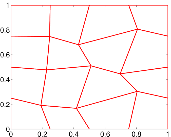
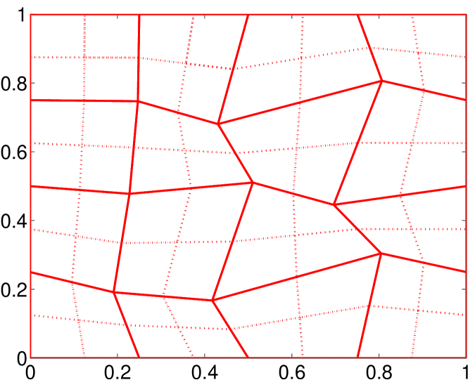
Fig. 2: Case 3: An initial mesh (Left) and its refinement (Right).

Table 4: Case 3. Convergence rate on deformed rectangles.

meshsize $h$	${|||}Q_{h}u-u_{h}{|||}$	$\|Q_{h}u-u_{h}\|$	$\|Q_{h}u-u_{h}\|_{\mathcal{E}_{h}}$
2.8790e-01	2.3056e+00	3.0235e-01	8.2633e-02
1.4395e-01	1.1673e+00	7.8108e-02	2.1396e-02
7.1974e-02	5.8473e-01	1.9652e-02	5.3912e-03
3.5987e-02	2.9241e-01	4.9203e-03	1.3503e-03
1.7993e-02	1.4619e-01	1.2445e-03	3.3774e-04
8.9967e-03	7.3095e-02	3.1112e-04	8.4445e-05
$O(h^{r}),r=$	0.9828	1.9618	1.9893

9.4 Case 4: WG-FEM on Meshes with Hanging Nodes

We solve the same problem as in Case 1 on deformed rectangular meshes with hanging nodes in the finite element partition. The initial mesh is shown as in Figure 3 (Left). The mesh on the right in Figure 3 is generated by following the same uniform refinement procedure as described in Case 3. It should be pointed out that the initial mesh has a hanging node in the usual definition.

For the finite element partition ${\mathcal{T}}_{h}$ with hanging nodes, the WG finite element method (19) must be modified as follows. For edge containing hanging nodes, the edge shall be further partitioned into smaller segments by using the hanging nodes. Then the corresponding finite element space defined on this edge will be piecewise linear functions with respect to the new partition; the finite element space on each element remains unchanged. For example, in Figure 4, the elements $K_{1}$, $K_{2}$, and $K_{3}$ share one hanging node $M$. In the WG finite element method, the edge $AB$ needs to be divided into two pieces: $AM$ and $MB$. The corresponding finite element function $v_{b}$ is taken as a piecewise linear function on edges $AM$ and $MB$. We point out that the refinement method adopted here may produce elements around the hanging node which are not shape regular as defined in Section 3. The numerical results are presented in Table 5. Readers are encouraged to draw conclusions from this table.

Table 5: Case 4: WG solutions and their convergence on deformed rectangular elements with hanging nodes.

meshsize $h$	${|||}Q_{h}u-u_{h}{|||}$	$\|Q_{h}u-u_{h}\|$	$\|Q_{h}u-u_{h}\|_{\mathcal{E}_{h}}$
4.2512e-01	3.8064e+00	9.1677e-01	2.5509e-01
2.1256e-01	2.2593e+00	3.2970e-01	7.3355e-02
1.0628e-01	1.2308e+00	9.2302e-02	2.2037e-02
5.3140e-02	6.3470e-01	2.3300e-02	6.1413e-03
2.6570e-02	3.2104e-01	5.8376e-03	1.7649e-03
1.3285e-02	1.6129e-01	1.7094e-03	5.1822e-04
$O(h^{r}),r=$	0.9201	1.8508	1.7912

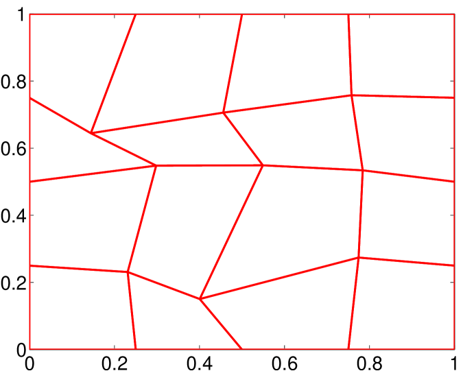
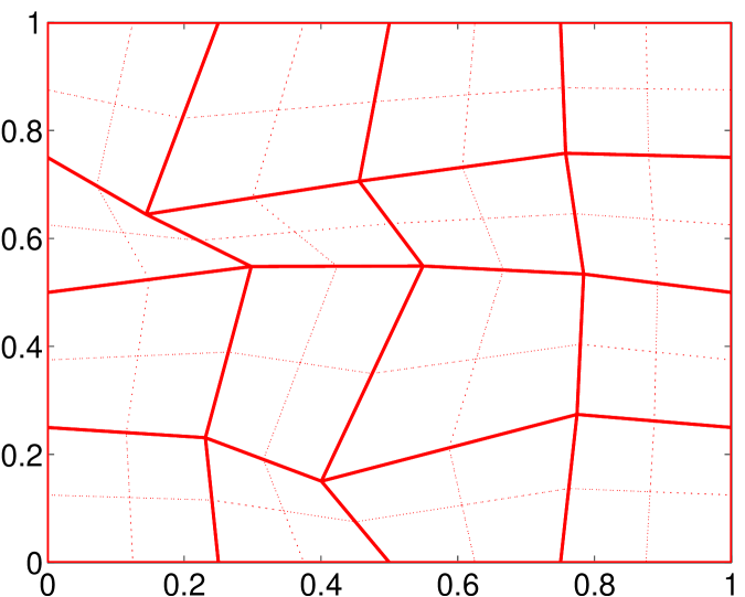
Fig. 3: Case 4: Mesh level 1 (Left) and Mesh level 2(Right).

Fig. 4: Case 4: Elements around a hanging node in the mesh.

References

• [1] D. N. Arnold and F. Brezzi, Mixed and nonconforming finite element methods: implementation, postprocessing and error estimates, RAIRO Mod l. Math. Anal. Num r., 19 (1985), pp. 7-32.
• [2] D. N. Arnold, F. Brezzi, B. Cockburn, and L. D. Marini, Unified analysis of discontinuous Galerkin methods for elliptic problems, SIAM J. Numer. Anal., 39 (2002), pp. 1749-1779.
• [3] I. Babus̆ka, The finite element method with Lagrange multipliers, Numer. Math., 20 (1973), pp. 179-192.
• [4] M. Berndt, K. Lipnikov, J. D. Moulton, and M. Shashkov, Convergence of mimetic finite difference discretizations of the diffusion equation, East-West J. Numer. Math. 9 (2001), pp. 253-294.
• [5] S. Brenner and R. Scott, The Mathematical Theory of Finite Element Mathods, Springer-Verlag, New York, 1994.
• [6] F. Brezzi, On the existence, uniqueness, and approximation of saddle point problems arising from Lagrange multipliers, RAIRO, 8 (1974), pp. 129-151.
• [7] F. Brezzi and M. Fortin, Mixed and Hybrid Finite Elements, Springer-Verlag, New York, 1991.
• [8] F. Brezzi, J. Douglas, Jr., R. Dur n and M. Fortin, Mixed finite elements for second order elliptic problems in three variables, Numer. Math., 51 (1987), pp. 237-250.
• [9] F. Brezzi, J. Douglas, Jr., and L.D. Marini, Two families of mixed finite elements for second order elliptic problems, Numer. Math., 47 (1985), pp. 217-235.
• [10] F. Brezzi, K. Lipnikov, and M. Shashkov, Convergence of the mimetic finite difference method for diffusion problems on polyhedral meshes, SIAM J. Numer. Anal., 43 (2005), No. 5, pp. 1872-1896.
• [11] P.G. Ciarlet, The Finite Element Method for Elliptic Problems, North-Holland, New York, 1978.
• [12] B. Cockburn, J. Gopalakrishnan, and R. Lazarov, Unified hybridization of discontinuous Galerkin, mixed, and continuous Galerkin methods for second order elliptic problems, SIAM J. Numer. Anal. 47 (2009), pp. 1319-1365.
• [13] D. Gilbarg and N. S. Trudinger, Elliptic Partial Differential Equations of Second Order, Springer- Verlag, Berlin-New York, 1977. MR 57:13109.
• [14] L. Mu, J. Wang, X. Ye, and S. Zhao, A numerical study on the weak Galerkin method for the Helmholtz equation with large wave numbers, arXiv:1111.0671v1, 2011.
• [15] L. Mu, J. Wang, G. Wei, X. Ye, and S. Zhao, Weak Galerkin methods for second order elliptic interface problems, arXiv:1201.6438v2, 2012.
• [16] P. Raviart and J. Thomas, A mixed finite element method for second order elliptic problems, Mathematical Aspects of the Finite Element Method, I. Galligani, E. Magenes, eds., Lectures Notes in Math. 606, Springer-Verlag, New York, 1977.
• [17] J. Wang and X. Ye, A weak Galerkin finite element method for second-order elliptic problems, arXiv:1104.2897v1, 2011.
• [18] J. Wang and X. Ye, A weak Galerkin mixed finite element method for second-order elliptic problems, arXiv:1202.3655v1, 2012.