Clustering analysis of high-redshift Luminous Red Galaxies in Stripe 82

Abstract

We present a clustering analysis of Luminous Red Galaxies (LRGs) in Stripe 82 from the Sloan Digital Sky Survey (SDSS). We study the angular two-point autocorrelation function, $w(\theta)$, of a selected sample of over 130 000 LRG candidates via colour-cut selections in $izK$ with the K band coverage coming from UKIRT Infrared Deep Sky Survey (UKIDSS) LAS. We have used the cross-correlation technique of Newman (2008) to establish the redshift distribution of the LRGs. Cross-correlating them with SDSS quasi-stellar objects (QSOs), MegaZ-LRGs and DEEP2 galaxies, implies an average redshift of the LRGs to be $z\approx 1$ with space density, $n_{g}\approx 3.20\pm 0.16\times 10^{-4}$ h³Mpc^-3. For $\theta\leq 10^{\prime}$ (corresponding to $\approx 10$ h^-1Mpc), the LRG $w(\theta)$ significantly deviates from a conventional single power-law as noted by previous clustering studies of highly biased and luminous galaxies. A double power-law with a break at $r_{b}\approx 2.4$h^-1Mpc fits the data better, with best-fit scale length, $r_{0,1}=7.63\pm 0.27$ h^-1Mpc and slope $\gamma_{1}=2.01\pm 0.02$ at small scales and $r_{0,2}=9.92\pm 0.40$ h^-1Mpc and $\gamma_{2}=1.64\pm 0.04$ at large scales. Due to the flat slope at large scales, we find that a standard $\Lambda$ cold dark matter ($\Lambda\rm$CDM) linear model is accepted only at $2-3\sigma$, with the best-fit bias factor, $b=2.74\pm 0.07$. We also fitted the halo occupation distribution (HOD) models to compare our measurements with the predictions of the dark matter clustering. The effective halo mass of Stripe 82 LRGs is estimated as $M_{\rm eff}=3.3\pm 0.6\times 10^{13}$ h^-1M_⊙. But at large scales, the current HOD models did not help explain the power excess in the clustering signal.

We then compare the $w(\theta)$ results to the results of Sawangwit et al. (2011) from three samples of photometrically selected LRGs at lower redshifts to measure clustering evolution. We find that a long-lived model may be a poorer fit than at lower redshifts, although this assumes that the Stripe 82 LRGs are luminosity-matched to the $AA\rm\Omega$ LRGs. We find stronger evidence for evolution in the form of the $z\approx 1$ LRG correlation function with the above flat 2-halo slope maintaining to $s\ga 50$h^-1Mpc. Applying the cross-correlation test of Ross et al. (2011), we find little evidence that the result is due to systematics. Otherwise it may represent evidence for primordial non-Gaussianity in the density perturbations at early times, with $f^{\rm local}_{\rm NL}=90\pm 30$.

1 Introduction

The statistical study of the clustering properties of massive galaxies provides important information about their formation and evolution which represent major questions for cosmology and astrophysics. The correlation function of galaxies remains a simple yet powerful tool for implementing such statistical clustering studies. (e.g. Peebles, 1980).

A lot of interest has been concentrated specifically on measuring the clustering correlation function of luminous red galaxies (LRGs) (Eisenstein et al., 2001) (see e.g Zehavi et al., 2005b; Blake, Collister, & Lahav, 2008; Ross et al., 2008; Wake et al., 2008; Sawangwit et al., 2011). LRGs are predominantly red massive early-type galaxies, intrinsically luminous ($\geq 3\rm L^{*}$) (Eisenstein et al., 2003; Loh & Strauss, 2006; Wake et al., 2006) and thought to lie in the most massive dark matter haloes. They are also strongly biased objects (Padmanabhan et al., 2007) and this coupled with their bright luminosity makes their clustering easy to detect out to high redshifts. For linear bias, the form of the LRG correlation function will trace that of the mass but even in this case the rate of correlation function evolution will depend on the bias model (e.g. Fry, 1996), which in turn depends on the galaxy formation process.

The passive evolution of the LRG LF and slow evolution of the LRG clustering (Wake et al., 2008; Sawangwit et al., 2011) seen in SDSS, 2SLAQ and $AA\rm\Omega$ Surveys already presents a challenge for hierarchical models of galaxy formation as predicted for a cold dark matter (CDM) universe. Since the LRG clustering evolution with redshift has been controversial, a major goal is to use the angular correlation function to test if the slow clustering evolution trend continues out to $z\approx 1$.

The uniformity of the LRG Spectral Energy Distributions (SEDs) with their 4000$\rm\AA\ CaII\ H\&K$ break, offer the ability to apply a colour-colour selection algorithm for our candidates. This technique has been successfully demonstrated primarily by Eisenstein et al. in SDSS in the analysis of LRG clustering at low redshift and then in 2SLAQ (Cannon et al., 2006) and $AA\rm\Omega$ (Ross et al., 2008) LRG surveys at higher redshifts. For our study, the available deep optical-IR ugrizJHK imaging data from the SDSS + UKIDSS LAS/DXS surveys in Stripe 82 will be used. This combination of NIR and deep optical imaging data, on a moderate sample size of area $\sim 200$ deg², results in a sample of $\approx 130\,000$ LRG candidates at redshift $z\approx 1$.

The main tool for our clustering analysis will be the two-point angular correlation function, $w(\theta)$, which has been frequently used in the past, usually in cases where detailed redshift information was not known. Hence, selecting Stripe 82 LRGs based on colour-magnitude criteria, correspond to a rough photometric redshift (photo-z) estimation based on the 4000$\rm\AA$ break shifting through the passbands. We shall apply the cross-correlation technique which was introduced by Newman (2008) to measure the redshift distribution, $n(z)$, of our photometrically selected samples. One of the main advantages of $w(\theta)$ is that it only needs the $n(z)$ of the sample and then through Limber’s formula (Limber, 1953) it can be related to the spatial two-point correlation function, $\xi(r)$.

In recent clustering studies, it was noted that the behaviour of $\xi(r)$, which has previously been successfully described by a single power-law of the form $\xi(r)=(r/r_{0})^{-\gamma}$, significantly deviates from such a power-law at $\sim 1$ h^-1Mpc. The break in the power-law, can be interpreted in the framework of a halo model, as arising from the transition between small scales (1-halo term) to larger than a single halo scales (2-halo term). Currently, our theoretical understanding of how galaxy clustering relates to the underlying dark matter is provided by the halo occupation distribution model (HOD, see, e.g Jing, Mo, & Boerner 1998; Ma & Fry 2000; Peacock & Smith 2000; Seljak 2000; Scoccimarro et al. 2001; Berlind & Weinberg 2002) via dark matter halo bias and halo mass function. Furthermore, the evolution of HOD can also give an insight into how certain galaxy populations evolve over cosmic time (White et al., 2007; Seo, Eisenstein, & Zehavi, 2008; Wake et al., 2008; Sawangwit et al., 2011).

The outline of this paper is as follows. In Section 2, we briefly describe the SDSS and UKIDSS data used in this paper, while in Section 3 we describe the angular function correlation function estimators and their statistical uncertainties. In Section 4, we estimate the redshift distribution through cross-correlations and then present the correlation results together with their power-law fits, $\Lambda\rm$CDM model and a halo model in Section 5. Section 6 is devoted to interpretation of the clustering evolution. In section 7, we explore potential systematic errors that might affect the large scale clustering signal. We then argue that, if real, an observed large-scale clustering excess may be due to the scale-dependent bias caused by primordial non-Gaussianity and compare our results to other previous works in Section 8. Finally, in Section 9 we summarize and conclude our findings.

Throughout this paper, we use a flat $\Lambda$-dominated cosmology with $\Omega_{m}=0.27$, $H_{0}=100h\ \rm kms^{-1}Mpc^{-1}$, h=0.7, $\sigma_{8}=0.8$ and magnitudes are given in the AB system unless otherwise stated.

2 DATA

2.1 LRG sample selection

We perform a $K$-band selection of high redshift LRGs in Stripe 82 based on the combined optical and IR imaging data, ugrizJHK, from SDSS DR7 (Abazajian et al., 2009) and UKIDSS LAS surveys (Lawrence et al., 2007; Warren et al., 2007), respectively. In previous studies, gri and riz colours have been used to select low to medium redshift LRGs, such as SDSS (Eisenstein et al., 2001), 2SLAQ (Cannon et al., 2006) and AA$\Omega$ (Ross et al., 2008) LRGs surveys up to $z\approx 0.7$. In this work we aim to study LRGs at $z\approx 1$, thus we use the izK colour magnitude limits for our selection in order to sample the 4000$\rm\AA\ CaII\ H\&K$ break of the LRGs’ SED as it moves across the photometric filters (Fukugita et al. 1996; Smith et al. 2002) taking advantage of the NIR photometry coverage from UKIDSS LAS. Coupling the UKIDSS LAS to $K_{Vega}\leq 18$ with the SDSS ugriz imaging to $i_{AB}<22.5$ in Stripe 82 produces an unrivaled combination of survey area and depth. Our selection criteria are :

$$\begin{array}[]{l}\displaystyle\rm SDSS\ Best\ Imaging\\ \displaystyle z-K+0.9(i-z)\geq 1.8,\ Pri\ A\sim 700deg^{-2}\\ \displaystyle z-K+0.9(i-z)\geq 2.3,\ Pri\ B\sim 240deg^{-2}\\ \displaystyle z-K-0.9(i-z)\geq-0.2\\ \displaystyle-0.5\leq i-z\leq 1.7\\ \displaystyle z-K\leq 4.0\\ \displaystyle 17.0\leq K\leq 18\\ \displaystyle z\leq 22.0.\end{array}$$ (1)

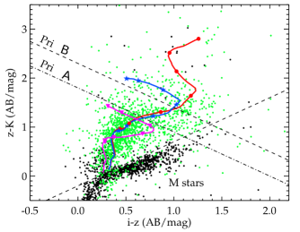
Figure 1: iz vs zK colour-colour plot. Priority A and B correspond to the $\sim 700\rm deg^{-2}$ and $\sim\rm 240deg^{-2}$ LRG samples, respectively. Objects with $J-K<1.3$ which is typical for M stars are plotted as black circles where as those with $J-K\geq 1.3$ are plotted in green. Evolutionary tracks for single burst (red line) and $\tau=1\rm Gyr$ (blue line) are overplotted from $z=0$ to 1.6 with symbols indicate $z$ interval of 0.2. The evolutionary track of late type galaxies (magenta line) is also shown for comparison.

The photometric selection of LRGs at $z>1$ requires a combination of optical and NIR photometry as the $4000\rm\AA$ band straddles the z band. The selection of high-redshift LRGs is done on the basis of SDSS $iz$ photometric data and the LAS $K$ band data (Fig. 1). LRG evolutionary models of Bruzual & Charlot (2003) are overplotted for single burst and $\tau=1\rm Gyr$ galaxy models indicating the izk plane area where we should apply our selections in order to study the high-z LRG candidates.

Late-type star contamination is a major problem in selecting a photometric sample of $z\approx 1$ LRGs. Here the $z-K$ colour also helps to distinguish the M stars colour locus from those of galaxies. From Fig.1, we see that most of the M stars lie at the bottom of the $izK$ colour plane. We identify these M stars by assuming their typical NIR colour, $J-K<1.3$. However, this means that our selection criteria must involve $J$ band data and would reduce the sky coverage due to the data availability. Therefore we choose to exclude these M stars by applying a cut in $izK$ colour plane with the condition $z-K-0.9(i-z)\geq-0.2$ in Eq. 1.

All magnitudes and colours are given in SDSS AB system and are corrected for extinction using the Galactic dust map of Schlegel, Finkbeiner, & Davis (1998). All colours described below refer to the differences in ‘model’ magnitudes (see Lupton et al., 2001, for a review on model magnitudes) unless otherwise stated.

Applying the above selection criteria (Eq. 1) on the SDSS DR7, we have two main LRG samples with a total observed area (after masking) of $\approx 200\rm deg^{2}$. The first sample has 130819 LRGs candidates with a sky surface density of $\approx 700\rm deg^{-2}$ and the second one 44543 with a sky density of $\approx 240\rm deg^{-2}$. The $240\ \rm deg^{-2}$ LRG sample was selected in such a way to check if the redshift distribution implied by cross-correlations is higher than the $700\ \rm deg^{-2}$ LRG sample.

3 THE 2-POINT ANGULAR CORRELATION FUNCTION MEASUREMENTS AND ERRORS

3.1 $w(\theta)$ Estimators

The probability of finding a galaxy within a solid angle $\delta\Omega$ on the celestial plane of the sky at a distance $\theta$ from a randomly chosen object is given by(e.g. Peebles, 1980)

$$\delta P=n[1+w(\theta)]\delta\Omega,$$ (2)

where n is the mean number of objects per unit solid angle. The angular two-point correlation function (2PCF) in our case, actually calculates the excess probability of finding a galaxy compared to a uniform random point process.

Different estimators can be used to calculate $w(\theta)$, so to start with we use the minimum variance estimator from Landy & Szalay (1993),

$$\textit{w}_{LS}(\theta)=1+\left(\frac{N_{rd}(N_{rd}-1)}{N(N-1)}\right)\frac{DD(\theta)}{RR(\theta)}-2\left(\frac{N_{rd}}{N}\right)\frac{DR(\theta)}{RR(\theta)}$$ (3)

where $DD(\theta)$ is the number of LRG-LRG pairs, $DR(\theta)$ and $RR(\theta)$ are the numbers of LRG-random and random-random pairs, respectively with angular separation $\theta$ summed over the entire survey area. $N_{rd}$ is the total number of random points, $N$ is the total number of LRGs and $N_{rd}/N$ is the normalisation factor. For our calculation we used two LRG samples (as explained in § 2.1) with different sky density, thus the density of the random catalogue that we use is $\sim 20$ times and $\sim 60$ times the number of the real galaxies for the first and second LRG samples, respectively. Using a high number density random catalogue helps to ensure the extra shot noise is reduced as much as possible.

We also compute $w(\theta)$ by using the Hamilton (1993) estimator which does not depend on any normalisation and is given by,

$$\textit{w}_{HM}(\theta)=\frac{DD(\theta)\cdotp RR(\theta)}{DR(\theta)^{2}}-1.$$ (4)

The Landy-Szalay estimator when used with our samples gives negligibly different results to the Hamilton estimator. Note that the Landy-Szalay estimator is used throughout this work except in §7.1 where we used both estimators to test for any possible gradient in number density of our samples.

For the computation of the cross-correlations in §4 and §7 we use the estimator (Guo, Zehavi, & Zheng (2011)) :

$$\textit{w}_{cross}(\theta)=\frac{D_{G}D_{S}(\theta)-D_{G}R_{S}(\theta)-D_{S}R{D}(\theta)-R_{G}R_{S}(\theta)}{R_{G}R_{S}(\theta)}$$ (5)

where the subscript G and S stands for the contribution in the pairs of the quantities that are cross-correlated in each case.

3.2 Error Estimators

To determine statistical uncertainties in our methods, we used three different methods to estimate the errors on our measurements. Firstly, we calculated the error on $w(\theta)$ by using the Poisson estimate

$$\sigma_{Poi}=\frac{1+w(\theta)}{\sqrt{DD(\theta)}}.$$ (6)

Secondly, we used the field-to-field error which is given by

$$\sigma^{2}_{FtF}(\theta)=\frac{1}{N-1}\sum_{i=1}^{N}\frac{DR_{i}(\theta)}{DR(\theta)}[w_{i}(\theta)-w(\theta)]^{2},$$ (7)

where N is the total number of subfields, $w_{i}(\theta)$ is an angular correlation function estimated from the ith subfield and $w(\theta)$ is measured using the entire field. For this method we divide our main sample to 36 subfields of equal size $\sim 6\rm deg^{2}$. We also reduce the number of subfields down to 18 with sizes of $\sim 12deg^{2}$ as we want to test how the results could deviate by using different sets of subsamples. While Stripe 82 has only $\sim 2.5$deg height, our subfields with their $\sim 2.5$deg and $\sim 5$deg widths are a reasonable size for estimating the correlation function up to scales of $1-2$deg.

Our final method is jackknife resampling, which is actually a bootstrap method. This technique has been widely used in clustering analysis studies with correlation functions (see, e.g Scranton et al. 2002; Zehavi et al. 2005a; Ross et al. 2007; Norberg et al. 2009; Sawangwit et al. 2011). The jackknife errors are computed using the deviation of the $w(\theta)$ measured from the combined 35 subfields out of the 36 subfields (or 17 out of 18 when 18 subfields are used). The subfields are the same as used for the estimation of the field-to-field error above. $w(\theta)$ is calculated repeatedly, each time leaving out a different subfield and hence results in a total 36 (or 18) measurements. The jackknife error is then

$$\sigma^{2}_{JK}(\theta)=\sum_{i^{\prime}=1}^{N}\frac{DR_{i^{\prime}}(\theta)}{DR(\theta)}[w_{i^{\prime}}(\theta)-w(\theta)]^{2},$$ (8)

where $w_{i^{\prime}}(\theta)$ is a measurement using the whole sample except the ith subfield and $DR_{i^{\prime}}(\theta)/DR(\theta)$ is approximately 35/36 (or 17/18) with slight variation depending on the size of resampling field. A comparison of the error estimators can be seen in Fig. 2. Poisson errors are found to be much smaller compared to jackknife errors particularly at larger scales. Field-to-field errors give similar results as jackknife errors, except at $\theta\gtrsim 10^{\prime}$ where the FtF errors underestimate the true error due to missing cross-field pairs. Since the jackknife errors are better at a scale of order $100^{\prime}$ which are of prime interest here, these are the error estimators that will be used in this work unless otherwise stated.

When calculated in small survey areas, $w(\theta)$ can be affected be an ‘integral constraint’, $ic$. Normally $w(\theta)$ has a positive signal at small scales and if the surveyed area is sufficiently small, this will cause a negative bias in $w(\theta)$ at largest scales (Groth & Peebles, 1977), i.e. $w_{est}(\theta)=w(\theta)-ic$. The integral constraint can be calculated from (see e.g. Roche & Eales 1999):

$$ic=\frac{\sum RR(\theta)w_{model}(\theta)}{\sum RR(\theta)},$$ (9)

where for the $w_{model}(\theta)$ we assume the standard $\Lambda\textrm{CDM}$ model in the linear regime (§5.3). No integral constraint is initially applied to our full sample results as the expected magnitude of $ic$ is smaller than the $w(\theta)$ amplitudes at scales analysed in this paper. This position will be reviewed when we move on to discuss models with excess power at large scales in §7.

To provide robust and accurate results from the correlation functions, we are also interested in model fitting to the observed $w(\theta)$ (see in §5.2, §5.4 and §5.3). Hence, for model fitting we will use the covariance matrix, which is calculated by:

$$\begin{array}[]{l}\mathbf{C}_{ij}=\frac{N-1}{N}\sum_{i,j=1}^{N}[w(\theta_{i})-\overline{w(\theta_{i})}][w(\theta_{j})-\overline{w(\theta_{j})}]\end{array}$$ (10)

where the $w_{i}(\theta_{i})$ is the correlation function measurement value excluding the $i^{th}$ subsample and the factor $N-1$ corrects from the fact that the realizations are not independent (Myers et al. 2007; Norberg et al. 2009; Ross, Percival, & Brunner 2010; Crocce et al. 2011; Sawangwit et al. 2011). The jackknife errors are the square-root of the diagonal elements of the covariance matrix, so we can now calculate the correlation coefficient, which is defined in terms of the covariance,

$$\textbf{{r}}_{ij}=\frac{\textbf{{C}}_{ij}}{\sqrt{\textbf{{C}}_{ii}\cdot\textbf{{C}}_{jj}}}$$ (11)

where $\sigma^{2}_{i}=C_{ii}$ (see Fig. 3). We can see that the bins are strongly correlated at large scales. The covariance matrix is more stable when we use 36 Jackknife subfields instead of 18, so we will use only the covariance matrix for the case of 36 subfields.

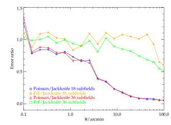
Figure 2: Comparison of the measured error ratios of the Jackknife, field-to-field and the Poisson errors for the $w(\theta)$ measurements of the $700\ deg^{-2}$ Stripe 82 LRG sample. Two different resampling sets have been used for the Jackknife and field-to-field errors, the first one based on 36 subfields and the second from 18 subfields.

Figure 3: The correlation coefficients $\textbf{{r}}_{ij}$, showing the level of correlation between each angular separation bin for the $700\ \rm deg^{-2}$ Stripe 82 LRG sample as calculated by using 36 subfields.

3.3 Angular Mask and Random Catalogue

To measure the observed angular correlation function we must compare the actual galaxy distribution with a catalogue of randomly distributed points. The random catalogue must follow the same geometry as the real galaxy catalogue, so for this reason we apply the same angular mask. The mask is constructed from ‘BEST’ DR7 imaging sky coverage. Furthermore, regions excluded in the quality holes defined as ‘BLEEDING’,  ‘TRAIL ’, ‘BRIGHT_STAR ’ and ‘HOLE’. The majority of the holes in the angular mask is from the lack of K coverage in Stripe 82. The final mask is applied to both our data and random catalogue (see Fig. 4).

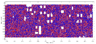
Figure 4: A fraction of the total $\sim 200\ \rm deg^{2}$ observed area in Stripe 82. LRG candidates (red) and random objects (blue), follow the same angular selection. Empty sky patches resulting from the lack of K-band coverage in the combined optical-IR data.

For generating the randomly distributed galaxies/points, we tried two different ways in order to modulate the surface density of the random points to follow the number density and the selection function of the real data. The selection function of the random catalogue mimics only the angular selection of the real data.

For the first method, we use a uniform density for the random points across the Stripe 82 area, so the normalization factor, $N_{rd}/N$, to be $\sim 20$ and $\sim 60$ for the $700\ \rm deg^{-2}$ and the $240\ \rm deg^{-2}$ LRG samples, respectively. A second random catalogue was created by dividing Stripe 82 into six smaller subfields ($15\times 2.5\rm deg^{2}$ each) and normalizing the density of random points to the density of galaxies within each subfield. The difference between the measured angular correlation function when we use the ‘global’ or the ‘local’ random catalogue is negligible. We will use the ‘global’ random catalogue for the clustering analysis. A $k$d-trees code (Moore et al., 2001) has been used to minimise the computation time required in the pair counting procedure.

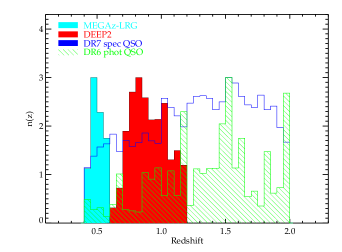
Figure 5: Normalised redshift distributions of MEGAz-LRGs, DEEP2 galaxies and SDSS QSOs in Stripe 82 that are used in the cross-correlations with the LRG samples.

4 LRG N(z) via Cross-Correlations

Even if the redshift of individual galaxies is not available, the 3-D clustering information can yet be recovered if the sample’s redshift distribution, n(z), is known. This can be achieved using Limber’s inversion equation (Limber, 1953) which can project the spatial galaxy correlation function, $\xi(r)$, to the angular correlation function given the n(z) of the sample:

$$w(\theta)=2\int_{0}^{\infty}dxf(x)^{2}\int_{0}^{\infty}du\ \xi(r=(u^{2}+x^{2}\theta^{2})^{1/2})$$ (12)

where f(x) is the galaxy redshift selection function. For our photometric selected LRG samples, only a very small fraction has a measured redshift, thus it is vital to estimate the n(z) of the Stripe 82 LRG samples.

One method for estimating the redshift distribution of the sample could be based on the various popular programs that derive photometric redshifts (photo-z’s). Photo-z estimates are based on the deep multi-band photometry coverage, and work by tracing some specific spectral features across the combination of filters which are then compared with different type of objects SED templates. Indeed, our izK selection is a rough photo-z cut as we follow the movement of the $4000\rm\AA$ break across the selected bands. In order to use the angular correlation function and the information that is encoded we need the n(z) of our sample, hence we follow the technique of Newman (2008) for reconstructing the LRG redshift distribution from cross-correlations.

4.1 Redshift distribution reconstruction

We employ Newman’s method, which is about determining the underlying redshift distribution of a sample of objects (LRGs in our case) through cross-correlation with a sample of known redshift distribution. By cross-correlating the sample (or samples) with known redshift and the sample under consideration, if both samples lie at the same distance, this will give a strong clustering signal. If the two samples that we are cross-correlating are separated and are at different $z$ distances, no cross-correlation signal will result. Thus, through the cross-correlations we can infer our photometrically selected LRG sample z ranges.

Following Newman (2008) the probability distribution function of the redshift of the Stripe 82 LRG samples, $\phi_{p}(z)$, is:

$$\phi_{p}(z)=w(z)\frac{3-\gamma}{2\pi}\frac{d_{A}(z)^{2}dl/dz}{H(\gamma)r_{0,sp}^{\gamma}r_{max}^{3-\gamma}}$$ (13)

where $w(z)$ is the integrated cross correlation function, $w_{sp}(\theta,z)$, of the LRG photometric samples with the samples of known spectroscopic redshift (see §4.2), $H(\gamma)=\Gamma(1/2)\Gamma((\gamma-1)/2)/\Gamma(\gamma/2)$ where $\Gamma(\chi)$ is the Gamma function, $d_{A}$ is the comoving angular distance and $dl$ is the comoving distance at redshift z. The comoving distance $r_{max}$ corresponds to the maximum angle at given redshift, which must be large enough to avoid nonlinear biasing effects.

To derive $\phi_{p}(z)$ via Eq. 13 we must estimate $w_{sp}(\theta,z)\sim\phi_{p}(z)\ r_{0,sp}^{\gamma_{sp}}$, since the angular size distance, $d_{A}(z)$ and the comoving distance $l(z)$ are given by the assumed cosmology. Thus we now require only knowledge of the $\gamma_{sp}$ and $r_{0,sp}$ parameters as function of redshift. Fortunately under the assumption of linear biasing, the cross-correlation of the two samples under consideration is the result of the geometric mean of the autocorrelation functions of the samples, i.e. $\xi_{sp}=(\xi_{ss}\xi_{pp})^{1\over 2}$, hence we can use the information provided by autocorrelation measurements for each sample to break the degeneracy between correlation strength and redshift distribution.

Newman investigates the effect of systematics such as: different cosmologies, bias evolution, errors from the autocorrelation measurements and field-to-field zero points variations in the final redshift probability distribution result. These issues could be more important in the case of future photometric surveys aimed at placing constraints on the equation of dark energy.

4.2 Cross-Correlation data sets

Newman’s angular cross-correlation technique requires the use of a data sample with known spectroscopic, or sufficiently accurate photometric, redshifts. For this reason we use a variety of samples with confirmed spectroscopic and photometric redshifts for the cross-correlations with Stripe 82 LRGs. The data samples that we use are: DEEP2 DR3 galaxies (Davis et al., 2003, 2007) , MegaZ-LRGs (Collister et al., 2007), SDSS DR6 QSOs (Richards et al., 2009) and SDSS DR7 QSOs (Schneider et al., 2010). In Fig. 5 we show the normalised redshift distributions of all the samples and in Table 1 we present the number of objects in each redshift bin.

Table 1: Number of objects in each separate redshift-bin used for the cross-correlations with Stripe 82 LRGs

	sample
	DEEP2	MegaZ-LRGs	DR6 Photometric Sample	DR7 Spectroscopic sample
redshift
0.4 - 0.6	-	30503	436	456
0.6 - 0.8	3152	-	695	526
0.8 - 1.0	5512	-	1199	547
1.0 - 1.2	3620	-	1630	729
1.2 - 1.4	-	-	1312	820
1.4 - 1.6	-	-	2646	854
1.6 - 1.8	-	-	1193	803
1.8 - 2.0	-	-	1990	668

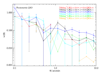
(a)

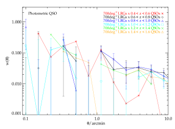
(b)

Figure 6: (a): Cross-correlation measurements of the $700\ \rm deg^{-2}$ Stripe 82 LRG sample with spectroscopic SDSS QSOs. (b): Same as (a) but now photometric SDSS QSOs are involved in the cross-correlations. Measurement uncertainties are $1\sigma$ jackknife errors.

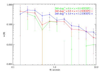
(a)

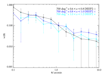
(b)

Figure 7: Cross-correlation measurements of the $240\ \rm deg^{-2}$ and $700\ \rm deg^{-2}$ Stripe 82 LRG samples with DEEP2 galaxies in (a) and (b), respectively. Uncertainties are $1\sigma$ jackknife errors.

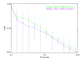
Figure 8: Cross-correlation measurements of the $700\ \rm deg^{-2}$ (green diamond) and $240\ \rm deg^{-2}$ (purple star) Stripe 82 LRGs with MEGAz-LRGs, along with $1\sigma$ jackknife errors.

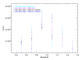
(a)

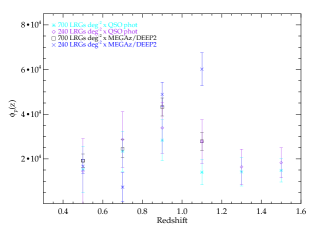
(b)

Figure 9: (a) The probability distribution function of the redshift, $\phi_{p}(z)$, of the $700\ \rm deg^{-2}$ and $240\ \rm deg^{-2}$ Stripe 82 LRGs as estimated through cross-correlations with MEGAz-LRGs, DEEP2 galaxies and spectroscopic SDSS QSOs. (b) Same as in (a) but now using photometric SDSS QSOs instead of spectroscopic in the cross-correlations. Error bars shown in both cases are $1\sigma$ jackknife summed up to $6^{\prime}$.

By using the above data sets for cross-correlation we satisfy the principal requirements of Newman’s method, with the most important being that the sky coverage of the data sets overlap the Stripe 82 LRGs. It must be mentioned though that not all the redshift surveys have the same sky coverage as Stripe 82 LRGs, so we reconstruct two redshift distributions via the cross-correlations providing us with the opportunity to check how much the n(z) cross-correlation technique is affected by area selection. One $n(z)$ is reconstructed by using all the data sets, the other $n(z)$ by using only SDSS QSOs in the cross-correlations.

4.2.1 SDSS DR6 $\&$ DR7 QSOs

QSO surveys are the main samples that we used for our cross-correlation measurements and they span the redshift range $0.4\leq z\leq 2.0$. When we refer to QSO data sets, we separate them into spectroscopic and photometric samples.

For the spectroscopic QSO sample we use the fifth edition of the SDSS Quasar Catalog, which is based on the SDSS DR7 (Schneider et al., 2010). The original data set contains 105,783 spectroscopically confirmed QSOs, from which only 5,403 in Stripe 82 have been used at $0.4\leq z\leq 2.0$ for cross-correlations (Table 1) with $i<22$ ($\sim 28\%$ of QSOs at $i>20$).

The photometric QSO sample comes from the photometric imaging data of the SDSS DR6 (Richards et al., 2009). The parent catalogue contains $\sim 1,000,000$ QSOs candidates from which we use 11,101 with $i<21.3$ in Stripe 82 and in the same redshift range as the spectroscopic QSOs.

In Fig. 6 we plot the cross-correlations between the Stripe 82 LRGs and the SDSS QSOs. We show only the case for cross-correlations of the $700\ \rm deg^{-2}$ Stripe 82 LRG sample with the spectroscopic and photometric SDSS QSOs. Cross-correlation with the $240\ \rm deg^{-2}$ LRG sample does not differ much. Errors shown here and for the other cross-correlation cases are jackknife errors.

4.2.2 DEEP2 Sample

The next sample of galaxies that we use is DEEP2 DR3 galaxies (Davis et al., 2003, 2007). The survey coverage in Stripe 82 is $\sim 1.7\ \rm deg^{2}$ with $i<24$. Galaxies in DEEP2 are split in three redshift bins with 0.2 step in the redshift range $0.6\leq z\leq 1.2$. The redshift distribution of the DEEP2 DR3 sample is shown in Fig. 5, with 12,284 galaxies in total. In Fig. 7 we show the results of the cross-correlations of the $700\ \rm deg^{-2}$ and $240\ \rm deg^{-2}$ LRG samples with the DEEP2 galaxies in the three aforementioned redshift bins.

4.2.3 MegaZ-LRG sample

The last sample that we use are LRGs from the MegaZ-LRG photometric catalogue (Collister et al., 2007). MegaZ-LRGs are used only in the redshift range of $0.4\leq z\leq 0.6$ with $i<20$. This sample offers us the ability to check the clustering properties of our high-redshift LRG candidates with another sample of LRGs. The total number of MEGAz LRGs that we use for cross-correlations is 30,503. In Fig. 8 are shown the cross-correlations between the Stripe 82 LRGs and the MEGAz LRGs.

4.3 Cross-Correlation results for n(z)

Having estimated the clustering signal from the cross-correlations of the above samples, we proceed to the reconstruction of the redshift distribution of the photometrically selected Stripe 82 LRG candidates. To estimate the probability distribution function of the redshift, $\phi_{p}(z)$, for the high-z LRG candidates we use equation (13). The pair-weighted clustering signal of the cross-correlations has been integrated up to $\approx 6^{\prime}$ for each redshift bin.

In Fig. 9 we can see the two cases of the estimated probability distribution function of the redshift for the high-z LRG candidates. For the first case, $\phi_{p}(z)$ has been estimated by using the spectroscopic SDSS QSOs whereas in the other case, $\phi_{p}(z)$ is estimated using only the photometric SDSS QSOs (DEEP2 galaxies and MEGAz-LRGs are also always used). For both cases we plot the errors estimated for each point in the redshift bin from the contributed cross-correlated sample.

To estimate the redshift distribution, n(z), we use the weighted mean for the $\phi_{p}(z)$ in each redshift bin, calculated through :

$$n(z)=\frac{\displaystyle\sum_{i=1}^{k}(\phi_{p}(i)/\sigma_{i}^{2})}{\displaystyle\sum_{i=1}^{k}(1/\sigma_{i}^{2})},$$ (14)

where k is the total number of bins at that redshift, $\phi_{p}(i)$ is the measured probability distribution function of each cross-correlation data set in the ith bin and $\sigma_{i}$ the error on that measurement.

The spectroscopic QSO $\phi_{p}(z)$ in Fig. 9a compared to the photo-z case in Fig. 9b, gives increased probability at $z\sim 1$. This may be explained by the SDSS QSO spectroscopic redshifts being more precise. For this reason, in our analysis and in fitting models to our $w(\theta)$ results, we will use only the spectroscopic n(z) for higher accuracy.

In Fig. 10 we plot the normalized redshift distribution of the $240\ \rm deg^{-2}$ and $700\ \rm deg^{-2}$ LRGs samples as calculated from Eq. 13 - 14. When we selected the two LRG samples from the $izK$ colour-plane, we applied a redder selection for the $240\ \rm deg^{-2}$ sample (see Eq. 1), aiming for a sample with a slightly higher redshift peak in the distribution as predicted from the evolutionary tracks in Fig. 1. This small difference may be seen between the spectroscopic n(z) of the $700\ \rm deg^{-2}$ and $240\ \rm deg^{-2}$ samples where the bluer cut has an average of $z\sim 1$ where for the redder sample the average is $z\sim 1.1$. But since the $700\ \rm deg^{-2}$ LRG sample has higher statistical accuracy in the n(z) determination, the majority of our analysis will be focused in this sample.

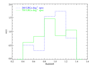
Figure 10: Weighted normalised redshift distribution of the Stripe 82 LRGs candidate samples when we use the spectroscopic SDSS QSOs along with the DEEP2 and MEGAz-LRG data sets. As expected the $700\ \rm deg^{-2}$ sample (solid green line) n(z) peak is lower when compared with the $240\ \rm deg^{-2}$ sample (dashed blue line).

5 RESULTS

5.1 Measured $w(\theta)$ and comparisons

In Fig. 11 we compare the observed angular correlation function of the $700\ \rm deg^{-2}$ LRG in Stripe 82 with Sawangwit et al. (2011) results. The $w(\theta)$ measurements are presented with 1$\sigma$ Jackknife errors.

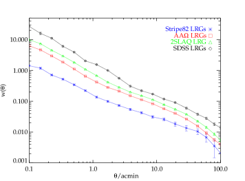
Figure 11: The angular correlation function, $w(\theta)$, from the $700\ \rm deg^{-2}$ Stripe 82 LRGs (star), AA$\Omega$ LRGs (square), 2SLAQ LRGs (triangle) and SDSS LRGs (diamond). At small scales all of the measurements show similar clustering behaviour, but at large scales the Stripe 82 clustering slope appears to be flatter than the lower $z$ samples.

The work of Sawangwit et al. involved three LRG data sets at $z\leq 1$ :

1. SDSS LRGs at $z\sim 0.35$

2. 2SLAQ LRGs $z\sim 0.55$

3. AA$\Omega$ LRGs $z\sim 0.68$

From Fig. 11 we can see that at small scales, $\theta\la 1^{\prime}$, the clustering trend for all the samples is similar but with decreasing amplitude for increasing redshift. At larger scales, we note that the $w(\theta)$ of the Stripe 82 LRGs seems to have a flatter slope than the other samples, departing from the expected behaviour for the correlation function.

Further comparisons below with the LRG clustering results of Sawangwit et al. will focus on the slope and amplitude of the $w(\theta)$ results, with an initial view to interpret any changes in terms of evolution. It is therefore of interest to see how the Stripe 82 sample match to the LRG samples used in previous studies in terms of luminosity and comoving space density.

A pair-weighted galaxy number density is given by (see e.g. Ross & Brunner, 2009) :

$$n_{g}=\int dz\frac{H(z)n(z)}{\Omega_{obs}\ c\ l^{2}(z)}\times n^{2}(z)\Big{/}\int dzn^{2}(z)$$ (15)

where $\Omega_{obs}$ is the observed area of the sky, $l(z)$ is the comoving distance to redshift $z$ and $c$ is the speed of light. The observed space density for the 700deg^-2 Stripe 82 sample is found to be $\approx 3.20\pm 0.16\times 10^{-4}\rm h^{3}Mpc^{-3}$. The quoted $1\sigma$ error has been estimated from the difference of the number density as calculated through Eq. 15 and by converting Fig. 10 into a plot of number density as a function of z (by dividing its bin by its corresponding volume).

Within the uncertainties of our $n(z)$, the 700deg^-2 sample appears to have similar space density to that of the AA$\Omega$ LRG sample (see Table 2 in §5.2). However, in this study we do not yet have redshift information for individual LRGs, not even for a subset of the sample. Hence it is more uncertain if our sample has similar luminosity as the LRG samples used by Sawangwit et al. (2011). We therefore take the fact that the samples are number-density matched to imply that they are also approximately luminosity matched which may turn out to be a reasonable assumption (see e.g. Sawangwit et al. 2011). This then should enable us to compare the clustering slopes and amplitudes of the AA$\Omega$ and Stripe 82 and infer any evolution independently of luminosity dependence.

5.2 $w(\theta)$ and power-law fits

Our first aim here is to fit power-laws to the Stripe 82 $w(\theta)$ to provide a simple parameterisation of the results. Our second aim is to make comparisons of the 3-D correlation amplitudes and slopes to measure evolution. Both aims will require application of Limber’s formula to relate the 2-D and 3-D correlation functions.

We begin by noting that the simplest function fitted to correlation functions is a single power-law with amplitude $r_{0}$ and slope $\gamma$. In previous studies, the spatial correlation function has been frequently described by a power-law of the form:

$$\xi(r)=\left(\frac{r}{r_{0}}\right)^{-\gamma}.$$ (16)

The angular correlation function as a projection of $\xi(r)$ can be written as $w(\theta)=\alpha\theta^{1-\gamma}$, commonly with a slope fixed at $\gamma=1.8$. The amplitude of the angular correlation function, $\alpha$, can be related with the correlation length $r_{0}$ through Limber’s formula (Eq. 12) using the equation (Blake, Collister, & Lahav, 2008):

$$\alpha=C_{\gamma}\ r_{0}^{\gamma}\int dz\ n(z)^{2}\left(\frac{dx}{dz}\right)^{-1}x(z)^{1-\gamma},$$ (17)

where $n(z)$ is the redshift distribution, $x(z)$ is the comoving radial coordinate at redshift z and the numerical factor $C_{\gamma}=\Gamma\left(\frac{1}{2}\right)\Gamma\left(\frac{\gamma}{2}-\frac{1}{2}\right)/\Gamma\left(\frac{\gamma}{2}\right)$.

Table 2: Best fit parameters for the single and double power-law fits to the angular correlation function.

Sample	$\bar{z}$	$n_{\rm{g}}$	Single power-law			Double power-law
		$(h^{3}Mpc^{-3})$	$\gamma$	$r_{0}(h^{-1}\,\rm{Mpc})$	$\chi^{2}_{\rm{red}}$	$\gamma_{1,2}$	$r_{0,1,2}(h^{-1}\,\rm{Mpc})$	$r_{b}(h^{-1}\,\rm{Mpc})$	$\chi^{2}_{\rm{red}}$
AA$\Omega$ LRGs	0.68	$2.7\times 10^{-4}$	$1.96\pm 0.01$	$7.56\pm 0.03$	42.8	$2.14\pm 0.01$	$5.96\pm 0.03$	1.3	3.4
($110deg^{-2}$)						$1.81\pm 0.02$	$7.84\pm 0.04$
Stripe82 LRGs	1.0	$3.20\pm 0.16\times 10^{-4}$	$2.01\pm 0.01$	$7.54\pm 0.16$	5.89	$2.01\pm 0.02$	$7.63\pm 0.27$	2.38	3.65
($700\ deg^{-2}$)						$1.64\pm 0.04$	$9.92\pm 0.40$

A deviation from a single power law at $\sim 1\rm h^{-1}Mpc$ has been measured in previous studies (Shanks et al., 1983; Blake, Collister, & Lahav, 2008; Ross et al., 2008; Kim et al., 2011; Sawangwit et al., 2011) and can be explained by the the 1-halo and 2-halo terms imprinted in the clustering signal under the assumption of the halo model (see §5.4). To parameterise the clustering characteristics of our sample, we fit a single-power law and a double-power law to our measured angular correlation function. The double power-law form is given as:

$$w_{1}(\theta)=\left(\frac{\theta}{\theta_{0,1}}\right)^{1-\gamma_{1}}(\theta<\theta_{b})$$ (18)

$$w_{2}(\theta)=\left(\frac{\theta}{\theta_{0,2}}\right)^{1-\gamma_{2}}(\theta\geq\theta_{b})$$ (19)

with $\theta_{b}$ to be the break point at $\approx 1.2^{\prime}$ where the power-law slope changes from being steeper at small scales ($<1.2^{\prime}$), to flatter at large scales.

The power-laws are fitted in the range $0.1^{\prime}<\theta<30^{\prime}$ using the $\chi^{2}$-minimization with the full covariance matrix constructed from the jackknife resampling (see §3.2):

$$\chi^{2}=\sum_{i,j=1}^{N}\Delta w(\theta_{i})\textbf{{C}}_{ij}^{-1}\Delta w(\theta_{j})$$ (20)

where $N$ is the number of angular bins, $\Delta w(\theta_{i})$ is the difference between the measured angular correlation function and the model for the $i$th bin, and $\textbf{{C}}_{ij}^{-1}$ is the inverse of the covariance matrix.

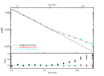
Figure 12: The best-fit single power law (diamond) and double power law (triangle), for the $700\ \rm deg^{-2}$ LRGs candidates overplotted on the angular correlation function (square) with the $1\sigma$ Jackknife error. Lower panel shows the fitting residuals.

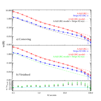
Figure 13: a) The AA$\Omega$ LRG raw $w(\theta)$ measurements (red square) with predictions from comoving evolution model (dashed red line), using the best-fit double power-law $r_{0}-\gamma$ values with Limber’s formula as Sawangwit et al. (2011) calculated. We then evolve the AA$\Omega$ best-fits utilising the estimated $700\ \rm deg^{-2}$ Stripe 82 LRG n(z) under the assumption of comoving evolution (dashed-dot black line) clustering. The observed Stripe 82 LRG $w(\theta$) is shown as well (blue star). b) Same raw measurements as above, but now compared to the virialised evolution clustering model. Stripe 82 LRG $w(\theta)$ measurements are described more accurate with comoving evolution at small and large scales compared to virialised evolution as it can been seen from the lower panel, where are plotted the residuals of the observed Stripe 82 $w(\theta)$ versus the comoving evolution (black star) and virialised evolution (green star) models, respectively.

For the single power-law, our best-fit spatial clustering length and clustering slope pair from Limber’s formula are measured to be $r_{0}=7.54\pm 0.16\rm h^{-1}Mpc$ and $\gamma=2.01\pm 0.01$ with associated reduced $\chi^{2}_{red}=5.89$. The $r_{0}-\gamma$ pairs for the double power-law are $r_{0,1}=7.63\pm 0.27\rm h^{-1}Mpc$ and $\gamma_{1}=2.01\pm 0.02$ at small scales and $r_{0,2}=9.92\pm 0.40\rm h^{-1}Mpc$ and $\gamma_{2}=1.64\pm 0.04$ at large scales with a reduced $\chi^{2}_{red}=3.65$. From the intersection of the 2 power law for $\xi(r)$, we have calculated the break scale, $r_{b}=2.38\rm h^{-1}Mpc$. This is higher than the $r_{b}=1.3-2.2\rm h^{-1}Mpc$ estimated from the SDSS, 2SLAQ and $\textrm{AA}\Omega$ LRG surveys (Sawangwit et al., 2011).

In Fig. 12 we show the data points including the $1\sigma$ Jackknife errors with the best-fitting power laws where the largest scale considered in the fitting was $\theta<30^{\prime}$, which corresponds to $r\la 20h^{-1}Mpc$ at $z\sim 1$ for the $700\ deg^{-2}$ LRG sample. Fig. 12 confirms that the double power-law clearly gives a better fit to the data than the single power-law. Note that in the case of the single power-law and the double power-law at small scales, our results give $r_{0}-\gamma$ values consistent with outcomes from previous studies. However, at large scales the Stripe 82 slope ($\gamma_{2}=1.64\pm 0.04$) is significantly flatter than the AA$\Omega$ result ($\gamma_{2}=1.81\pm 0.02$).

Fig. 13 shows the double power-law fits for AA$\Omega$ (dashed red lines) taken from Sawangwit et al. and then evolved (black and green dot-dashed lines) to the Stripe 82 depth using Eq. 17 under the assumptions of comoving and virialised clustering, respectively. We shall interpret the amplitude scaling in the discussion of evolution in §6.1 later. At this point we again note that the biggest discrepancy seems to be at large scales where the Stripe 82 slope is increasingly too flat relative to the AA$\Omega$ result. Fitted parameters are given in Table 2, where the best-fit power-law parameters for the $\textrm{AA}\Omega$ LRG sample (Sawangwit et al., 2011) are also presented for comparison.

We note here that Kim et al. (2011) studied the clustering of extreme red objects (EROs) at $1<z<2$ in the SA22 field and they report a similar change of the large scale slope. Gonzalez-Perez et al. (2011) tried to fit clustering predictions from semi-analytic simulations to the Kim et al. ERO $w(\theta)$ but found that the model underpredicts the clustering at large scales.

5.3 $\Lambda$CDM model fitting in the linear regime

Since the standard $\Lambda$CDM model was found to give a good fit to the lower redshift LRG samples of Sawangwit et al. (2011), we now check to see whether the flatter large-scale slope of the Stripe 82 LRG $w(\theta)$ leads to a statistically significant discrepancy with the $\Lambda\rm$CDM model at $z\approx 1$. We generate matter power spectra using the ‘CAMB’ software (Lewis, Challinor, & Lasenby, 2000), including the case of non-linear growth of structure correction. For this reason we use the ‘HALOFIT’ routine (Smith et al., 2003) in ‘CAMB’. Our models assume a $\Lambda$CDM Universe with $\Omega_{\Lambda}=0.73$, $\Omega_{m}=0.27$, $f_{baryon}=0.167$, $\sigma_{8}=0.8$, $h=0.7$ and $n_{s}=0.95$. Then we transform the matter power spectra to obtain the matter correlation function, $\xi_{\rm{m}}(r)$, using:

$$\xi_{\rm{m}}(r)=\frac{1}{2\pi^{2}}\int_{0}^{\infty}{P_{m}(k)k^{2}\frac{\ sin{kr}}{kr}}dk.$$ (21)

The relationship between the galaxy clustering and the underlying dark-matter clustering is given by the bias, $b_{g}$ :

$$b_{\rm{g}}^{2}(r)=\frac{\xi_{\rm{g}}(r)}{\xi_{\rm{m}}(r)}.$$ (22)

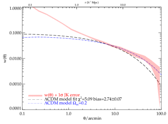
Figure 14: The best-fit spatially flat, $\Lambda\rm$CDM model assuming $\Omega_{m}=0.27$ compared to the observed $w(\theta)$ of Stripe 82 $700\ \rm deg^{-2}$ LRGs in the linear regime. The standard model cannot explain the large scale power excess in the angular correlation function of the Stripe 82 LRGs. The shaded area corresponds to $\pm 1\sigma$ jackknife error. Also shown is a spatially flat $\Lambda\rm$CDM model with the same parameters as before except for a lower value of $\Omega_{m}=0.2$ and an arbitrary normalisation. The $\Omega_{m}=0.2$ model appears to give a better fit than the standard $\Omega_{m}=0.27$ model.

As we are interested in the linear regime, we fit the projected $\xi_{\rm{m}}(r)$ to the Stripe 82 LRG $w(\theta)$ in the range $4^{\prime}\la\theta\la 45^{\prime}$, corresponding to comoving separations $3\la r\la 30\rm h^{-1}$Mpc. By fitting the model predictions to the measured $w(\theta)$ it will result with the best linear bias factor, the only free parameter in this case. For our fitting, the $\chi^{2}$-minimization with the full covariance matrix constructed from the jackknife resampling (see §3.2) has been used.

The best-fit linear bias parameter is estimated to be $b=2.74\pm 0.07$ with $\chi_{red}^{2}=5.09$. The upper limit of our fitted range in $\theta$ was varied, while the lower limit stayed constant to avoid any contribution from the non-linear regime. Thus, for the range $\sim 4^{\prime}-30^{\prime}$ the best-fit bias is $b=2.8\pm 0.08$ with $\chi_{red}^{2}=4.72$ and at $\sim 4^{\prime}-60^{\prime}$ is $b=2.69\pm 0.07$ with $\chi_{red}^{2}=5.18$. In Fig. 14 we plot the LRG $w(\theta)$ with the $1\sigma$ error and the $\Lambda\rm$CDM model with the best-fit bias. For low values of the upper limit of the fitting range, the measured biases are in approximate agreement with other results in the literature. But in terms of the flat slope of $w(\theta)$ at large scales, the standard $\Lambda\rm$CDM linear model is inconsistent with the data at the $2-3\sigma$ level. One of the aims of the next section will be to see if a HOD model can explain the flat large-scale slope of the $z\approx 1$ Stripe 82 LRGs.

5.4 Halo model analysis

We are going to use the approach of the halo model (see Cooray & Sheth, 2002, for a review) of galaxy clustering to finally fit our angular correlation function results. Under the halo-model framework we can examine the way the dark matter haloes are populated by galaxies through the Halo Occupation Distribution (HOD). Various studies have used this model to fit their results (e.g. Masjedi et al., 2006; White et al., 2007; Blake, Collister, & Lahav, 2008; Wake et al., 2008; Brown et al., 2008; Ross & Brunner, 2009; Zheng et al., 2009; Sawangwit et al., 2011; Gonzalez-Perez et al., 2011) as a way to explain the galaxy correlation function and gain insight into their evolution. Specifically, we shall investigate whether the HOD model may be able to explain the flatter slope of the correlation function observed here.

In the halo model, the clustering of galaxies is expressed by the contribution of number of pairs of galaxies within the same dark matter halo (one-halo term, $\xi{1}$) and to pairs of galaxies in two separate haloes (two-halo term) :

$$\xi(r)=\xi_{1h}(r)+\xi_{2h}(r).$$ (23)

The 1-halo term dominates on small scales $\lesssim 1Mpc$.

The fundamental ingridient in the HOD formalism of galaxy bias is the probability distribution $P(N|M)$, for the number of galaxies N to hosted by a dark matter halo as a function of its mass M.

We use the so-called centre-satellite three-parameter HOD model (e.g. Seo, Eisenstein, & Zehavi, 2008; Wake et al., 2008; Sawangwit et al., 2011) which distinguishes between the central galaxy and the satellites in a halo. This separation has been shown in simulatations (Kravtsov et al., 2004) and has been commonly used in semi-analytic galaxy formation models in the last years (Baugh, 2006).

Different HODs are applied for the central and satellite galaxies. We assume that only haloes which host a central galaxy are able to host satellite galaxies. The fraction of haloes of mass M with centrals is modelled as:

$$\left<N_{\rm c}|M\right>={\rm{exp}}\left(\frac{-M_{\rm{min}}}{M}\right).$$ (24)

In such haloes, the number of satellite galaxies follows a Poisson distribution (Kravtsov et al., 2004) with mean:

$$\left<N_{\rm s}(M)\right>=\left(\frac{M}{M_{1}}\right)^{\alpha}.$$ (25)

To describe the distribution of the satellite galaxies around the halo centre we use the NFW profile (Navarro, Frenk, & White, 1997). So, the mean number of galaxies residing in a halo of mass $M$ is:

$$\left<N|M\right>=\left<N_{\rm c}|M\right>\times(1+\left<N_{\rm s}|M\right>.$$ (26)

and the predicted galaxy number density from the HOD is then:

$$n_{\rm{g}}=\int{\rm{d}}M\,n(M)\left<N|M\right>$$ (27)

where $n(M)$ is the halo mass function, where in our case we use the model of Sheth & Lemson (1999).

From the HOD we can derive useful quantities which are the central fraction :

$$F_{\rm cen}=\frac{\int\rm{d}M\,n(M)\left<N_{\rm c}(M)\right>}{\rm{d}M\,n(M)\left<N_{\rm c}(M)\right>\left[1+\left<N_{s}(M)\right>\right]},$$ (28)

and the satellite fraction of the galaxy population:

$$F_{\rm sat}=\frac{1}{n_{\rm{g}}}\int{\rm{d}}M\,n(M)\left<N_{\rm c}(M)\right>\left<N_{\rm s}|M\right>,$$ (29)

as $F_{sat}=1-F_{cen}$. We can also determine the effective mass, $M_{eff}$, of the HOD:

$$M_{\rm eff}=\frac{1}{n_{\rm{g}}}\int{\rm{d}}M\,n(M)M\left<N|M\right>,$$ (30)

and the effective large-scale bias:

$$b_{g}=\frac{1}{n_{\rm{g}}}\int{\rm{d}}M\,n(M)b(M)\left<N|M\right>,$$ (31)

where $b(M)$ is the halo bias, for which we use the ellipsoidal collapse model of Sheth, Mo, & Tormen (2001) and the improved parameters of Tinker et al. (2005).

Table 3: Best-fit HOD parameters.

Sample	$\bar{z}$	$M_{\rm min}$	$M_{1}$	$\alpha$	$n_{\rm{g}}$	$M_{\rm eff}$	$F_{\rm sat}$	$b_{\rm lin}$	$\chi^{2}_{\rm red}$
		($10^{13}h^{-1}M_{\odot}$)	($10^{13}h^{-1}M_{\odot}$)		$(10^{-4}h^{3}Mpc^{-3})$	($10^{13}h^{-1}M_{\odot}$)	(per cent)
AA$\Omega$	0.68	$1.02\pm 0.03$	$12.6\pm 1.0$	$1.50\pm 0.03$	$3.1\pm 0.4$	$3.0\pm 0.1$	$9.0\pm 0.09$	$2.08\pm 0.03$	13.6
Stripe82 $(10^{\prime})$	1.0	$3.09\pm 0.75$	$30.2\pm 6.7$	$2.38\pm 0.12$	$0.5\pm 0.3$	$4.0\pm 0.6$	$2.13\pm 1.0$	$3.01\pm 0.21$	2.4
Stripe82 $(30^{\prime})$	1.0	$2.57\pm 0.31$	$25.7\pm 3.1$	$2.28\pm 0.04$	$0.6\pm 0.2$	$3.6\pm 0.5$	$2.62\pm 0.07$	$2.90\pm 0.15$	2.3
Stripe82 $(45^{\prime})$	1.0	$2.19\pm 0.63$	$21.9\pm 5.6$	$2.24\pm 0.12$	$0.8\pm 0.3$	$3.3\pm 0.6$	$3.17\pm 0.10$	$2.81\pm 0.18$	3.1
Stripe82 $(60^{\prime}$)	1.0	$2.19\pm 0.21$	$21.9\pm 2.1$	$2.25\pm 0.05$	$0.8\pm 0.2$	$3.3\pm 0.3$	$3.17\pm 0.08$	$2.81\pm 0.10$	3.6

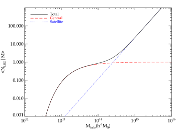
(a)

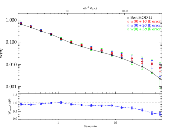
(b)

Figure 15: (a) The mean number of LRGs per halo as a function of halo mass at $z=1$. The total, central and satellite contributions are shown by the solid, dashed and dotted lines, respectively. (b) The measured angular correlation function $w(\theta)$ for the $700\ \rm deg^{-2}$ LRG sample with the best HOD fit (black star). The 1, 2 and $3\sigma$ Jackknife errors are shown in red, blue and green, respectively.

As the galaxy correlation function is the Fourier transform of the power spectrum, the 1-halo term and the 2-halo term of the clustering functions can be written as:

$$P(k)=P_{1{\rm h}}(k)+P_{2{\rm h}}(k).$$ (32)

Moreover the 1-halo term can be distinguished from the contribution of the central-satellite pairs, $P_{\rm cs}(k)$, and satellite-satellite pairs, $P_{\rm ss}(k)$, (see e.g. Skibba & Sheth, 2009):

$$P_{\rm cs}(k)=\frac{1}{n^{2}_{\rm g}}\int{\rm d}M\,n(M)2\left<N_{\rm c}|M\right>\left<N_{\rm s}|M\right>u\left<k|M\right>,$$ (33)

and

$$P_{\rm ss}(k)=\frac{1}{n^{2}_{\rm g}}\int{\rm d}M\,n(M)\left<N_{\rm c}|M\right>\left<N_{\rm s}|M\right>^{2}u\left<k|M\right>^{2},$$ (34)

where $u\rm\left<k|M\right>$ is the NFW density profile in Fourier space and we have simplified the number of satellite-satellite pairs $\left<N_{\rm s}(N_{\rm s}-1)|M\right>$ to $\left<N_{\rm s}|M\right>^{2}$ since the satellites are Poisson-distributed.

The 2-halo term is evaluated as:

$$P_{2{\rm h}}(k,r) = P_{\rm m}(k)\times\frac{1}{n_{\rm g}^{\prime 2}}$$ (35)

$$\times\left[\int_{0}^{M_{\rm lim}(r)}{\rm d}M\,n(M)b(M,r)\left<N(M)\right>u(k,M)\right]^{2},$$

where $P_{\rm m}(k)$ is a non-linear matter power spectrum. We derive the mass limit, $M_{\rm lim}(r)$, using the ‘$n_{\rm g}^{\prime}$-matched’ approximation of (Tinker et al., 2005), which accounts the effect of halo exclusion: different haloes cannot overlap. $n_{\rm g}^{\prime}$ is the restricted galaxy number density (Eq. B13 of Tinker et al. (2005)).

For the scale-dependent halo bias, $b(M,r)$, we use the model given by Tinker et al. (2005):

$$b^{2}(M,r)=b^{2}(M)\frac{\left[1+1.17\xi_{\rm m}(r)\right]^{1.49}}{\left[1+0.69\xi_{\rm m}(r)\right]^{2.09}},$$ (36)

where $\xi_{\rm m}(r)$ is the non-linear matter correlation function. For the 2-halo term, we need to correct the galaxy pairs from the restricted galaxy density to the entire galaxy population.

By using Limber’s formula to project the predicted spatial galaxy correlation function $\xi(r)$ to the angular correlation function $w(\theta)$ and we fit for a variety of the three-parameter halo model ($M_{min}$, $M_{1}$, $\alpha$).

The best-fit model for each of our sample is then determined from the minimum value of the $\chi^{2}$-statistic using the full covariance matrix. We use the full covariance matrix over the range $0.25^{\prime}<\theta<60^{\prime}$ in our fitting. Smaller scales are excluded in the fitting because any uncertainty in the $\xi(r)$ model can have a strong effect on $w(\theta)$ due to the projection. To determine the $1\sigma$ error on the fits, the region of parameter space from the best fits with $\delta\chi^{2}\leq 1$ ($1\sigma$ for 1 degree of freedom) is considered. For $b_{\rm lin}$, $M_{\rm eff}$, $F_{\rm sat}$ and $n_{\rm g}$ which depend on all the three main parameters, the considered region of the parameter space becomes $\delta\chi^{2}\leq 3.53$.

Fig. 15a shows the resulting best-fit HOD of the mean number of LRGs per halo along with the central and satellite contributions. The best-fitting values for $M_{\rm min}$, $M_{1}$ and $\alpha$ where $M_{min}=2.19\pm 0.63\times 10^{13}\rm h^{-1}M_{\odot}$, $M_{1}=21.9\pm 5.6\times 10^{13}\rm h^{-1}M_{\odot}$ and $\alpha=2.24\pm 0.12$, respectively. The associated values for $b_{\rm lin}$, $M_{\rm eff}$, $F_{\rm sat}$ and $n_{\rm g}$ are given in Table 3.

We see that the $\left<N|M\right>$ of the LRGs flatten at unity, as expected from the assumption satellite galaxies are hosted by halos with central galaxies. The LRGs as expected populate massive dark matter haloes with the masses $\approx 10^{13}-10^{14}\rm h^{-1}M_{\odot}$. With the fraction of LRGs that are satellites being less than $5\%$, we therefore find that $>95$% of LRGs are central galaxies in their dark matter haloes. The best fit linear bias, $b_{\rm lin}\approx 2.8$, agrees with the prediction from Sawangwit et al. (2011) in the case of a long lived model for the LRGs and indicates that the LRGs are highly biased tracers of the clustering pattern. The effective mass, $M_{\rm eff}\approx 3\times 10^{13}\rm h^{-1}M_{\odot}$, confirms that LRGs are hosted by the most massive dark matter haloes. Despite the fact that we use a higher redshift LRG sample, our best-fit HOD parameters are statistically not too dissimilar to those found in previous LRG studies (eg see Table 3).

In Fig. 15b we show the best-fit model for $w(\theta)$, compared to the data. The first thing we notice is that while at small scales the best-fit HOD are in good agreement with the $w(\theta)$ measurements, at large scales the model fits only at $2-3\sigma$. The flatter slope at large scales is responsible for that and we still are not able to say if this can be explained by evolution in the linear regime or any kind of systematic effect. In §7 we will check systematic errors that could affect our results.

Moreover, due to the high value of the best-fit reduced $\chi^{2}=3.1$, we also try to fit the HOD models at different scales by using 4 different maximum $\theta$ bins of the covariance matrix in our fits, which we present in Table 3. The fits at large scales did not improve and above $45^{\prime}$ there was not any change in the best-fit HOD measurements.

Considering the two-halo term in the HOD model, one can see that the bias in this regime is mostly scale-independent and the correction factor is in fact having the opposite effect on the slope. The scale-independent bias is simply the average of the halo bias, $b(M)$, weighted by the halo mass function and the mean number of galaxies hosted by the corresponding halo. One way to boost the large-scale amplitude is to increase $M_{\rm min}$ and therefore increase the mass range of the halo where most galaxies occupy and hence linear bias and amplitude of the two-halo term. However, to compensate for the increase numbers of satellite galaxies (and consequently small-scale clustering amplitude) one must also increase $M_{1}$, the mass at which a halo hosts one satellite galaxy on average. And in order to produce the overall flatter slope one needs to increase $M_{1}/M_{\rm min}$. However, this would still overpredict the clustering amplitude in the intermediate scales, $r\sim 5-10\ \rm h^{-1}Mpc$. Note that our best-fit HOD gives $M_{1}/M_{\rm min}\approx 10$, consistent with previous results for lower redshift LRGs of (Sawangwit et al., 2011) and (Wake et al., 2008). However, as noted earlier including $w(\theta)$ bins at larger and larger scales does not change the best-fit parameters which means that $M_{1}/M_{\rm min}$ also remains unchanged due to the reason discussed above. We therefore conclude that the HOD prescription in the framework of standard $\Lambda\rm$CDM cannot explain the observed large-scale slope in $w(\theta)$ of the $z\approx 1$ LRG sample.

6 Clustering Evolution

6.1 Intermediate scales

First, we compare the clustering of the $z\approx 1$ Stripe 82 LRG sample to the lower redshift $z\approx 0.68$ $AA\Omega$ LRG sample. We recall that these LRG samples have approximately the same space density and so should be approximately comparable. We follow Sawangwit et al. (2011) and by using our best-fit $r_{0}$ and $\gamma$ we make comparison with their data and models via the integrated correlation function in a $20\ \rm h^{-1}Mpc$ sphere, $\xi_{20}$.

$AA\Omega$ LRG results are described better with the long-lived model of Fry (1996). Fry’s model assumes no merging in the clustering evolution of the galaxies while they move within the gravitational potential, hence the comoving number density is kept constant. The bias evolution in such a model is given by:

$$b(z)=1+\frac{b(0)-1}{D(z)}$$ (37)

where D(z) is the linear growth factor.

However, the flat slope beyond 1h^-1Mpc causes a highly significant, $\approx 50$%, rise in $\xi_{20}$ above the $AA\Omega$ $\xi_{20}$ as we can see in Fig. 16 (see also Figs. 13a,b). If we assume that the 2 samples are matched then we would conclude that all of the models discussed by Sawangwit et al. (2011) were rejected.

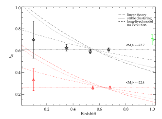
Figure 16: The LRG $\xi_{20}$ measurements as a function of redshift and luminosity from Sawangwit et al. (2011). Lowest redshift data are early-type galaxies from 2dFGRS (Norberg et al. 2002). Stars represent the brighter samples (SDSS, 2SLAQ* and $AA\Omega^{*}$-LRG), where the lower luminosity samples, triangles, have been lowered by 0.2 for clarity. The 700 deg^-2 Stripe 82 LRGs $\xi_{20}$ measurement is at $z=1$ (square).

One possibility is that the 700deg^-2 LRG sample is closer to the SDSS and $AA\Omega^{*}$ LRG space density of $1.1\times 10^{-4}$ h^-3Mpc^-3 because the LRG $\xi_{20}$ fits the extrapolated models better there. If so, then this would imply that the Stripe 82 LRG $n(z)$ width was underestimated in the cross-correlation procedure and this would then increase the deprojected amplitude of $\xi(r)$, suggesting that this explanation may not work. Similarly a larger correction for stellar contamination would also produce a higher Stripe 82 clustering amplitude. We do not believe that looking further into the evolution of the bias (Papageorgiou et al., 2012) and DMH is warranted until we understand the flat slope of the Stripe 82 $w(\theta)$ at large scales.

6.2 Small scales

At smaller scales ($r<1\ \rm h^{-1}Mpc$) the situation is less complicated by the flat large-scale slope. Here Sawangwit et al. found that a virialised model gave a better fit to the slightly faster evolution needed to fit the small-scale correlation function amplitudes than a comoving model. But in the present case, the scaling between the AA$\Omega$ and Stripe 82 LRGs in Fig. 13a,b, shows that here the comoving model is preferred at small scales over the faster virialised evolution. This fits with the more general picture of the Stripe 82 LRGs presenting a higher amplitude than expected all the way down to the smallest scales. Unfortunately the remaining uncertainty in the Stripe 82 LRG luminosity class is still too large to make definitive conclusions on this evolution possible.

6.2.1 HOD Evolution

Given the uncertainty in $\xi_{20}$ caused by the flat $w(\theta)$ slope on intermediate - large scales, we will extend further the studies at small-scales, using the HOD model to interpret the small-scale clustering signal of the LRGs. Based on the HOD fit at $z\approx 1$, we again follow Sawangwit et al. (2011), (and references therein) and test long-lived and merging models by comparing the predictions of these models to the SDSS HOD fit from Sawangwit et al.. These authors and also Wake et al. (2008) found that long-lived models were more strongly rejected at small scales ($r<1$ h^-1Mpc) than at intermediate-large scales.

Again we follow the approach of Wake et al. (2008)) and Sawangwit et al. (2011) who assumed a form for the conditional halo mass function Sheth & Tormen (2002) and a sub-Poisson distribution for the number of central galaxies in low-redshift haloes of mass $M$ such that

$$\left<N_{\rm c}(M)\right>=1-\left[1-\frac{C(M)}{N_{\rm max}}\right]^{N_{\rm max}},$$ (38)

where $N_{\rm max}={\rm int}(M/M_{\rm min})$,

$$C(M)=\int_{0}^{M}{\rm d}m\,N(m,M)\left<N_{\rm c}(m)\right>$$ (39)

and $N(m,M)$ is the expression of Sheth & Tormen (2002) for the conditional halo mass which generalize those of Lacey & Cole (1993). The mean number of satellite galaxies in the low-redshift haloes is then given by

$$\left<N_{\rm c}(M)\right>\left<N_{\rm s}(M)\right>=S(M)+f_{\rm no-merge}\left[C(M)-\left<N_{\rm c}(M)\right>\right],$$ (40)

where

$$S(M)=\int_{0}^{M}{\rm d}m\,N(m,M)\left<N_{\rm c}(m)\right>\left<N_{\rm s}(m)\right>.$$ (41)

and the main parameter is $f_{\rm no-merge}$ which is the fraction of un-merged low-$z$ satellite galaxies which were high-$z$ central galaxies.

This model is called ‘central-central mergers’ in Wake et al. (2008). More massive high-z central galaxies are more likely to merge with one another or the new central galaxy rather than satellite-satellite mergers.

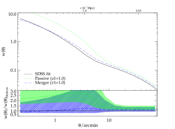
Figure 17: The predicted SDSS LRG $w(\theta)$’s at $z_{later}=0.35$ for the case of passively ($f_{\rm no-merge}=1$) evolving the best-fit HOD of Stripe 82 LRGs sample from $z_{earlier}=1$ and the case where central galaxies merging is allowed from $z_{earlier}=1$ ($f_{\rm no-merge}=0.21$), in green dot-dashed line and blue long-dashed line, respectively. The bottom panel shows the ratios of the evolved $w(\theta)$’s to the SDSS best-fit, the shaded regions signify the $1\sigma$ uncertainties.

Setting $f_{\rm no-merge}=1$ means that there is no merging of initial central galaxies in subsequently merged haloes, so it is similar to the passive/long-lived model. $f_{\rm no-merge}$ equals to 0 means that all the central galaxies in haloes at high redshift merge to form new central and/or satellite galaxies in the low redshift haloes. In the analysis below, we use the best-fit HOD model values as estimated for scales up to $45^{\prime}$ (see Table 3).

The $f_{\rm no-merge}=1$ case is shown as the $w(\theta)$ passive model in Fig. 17 and is clearly rejected by the data at $\theta\lesssim 10^{\prime}$(see lower panel). Best-fit HOD predictions of the satellite fraction in the case of the passively evolved LRGs from $z_{earlier}=1$ to $z_{later}=0.35$ is $F_{sat}=18.6\pm 2.5\%$ whereas Sawangwit et al. measured $F_{sat}=18\pm 1$% for a brighter selection of LRGs at $z_{earlier}=0.68$. We see that both these results, for the long-lived model, are significantly higher compared to the best-fit SDSS HOD, $F_{sat}=8.1\pm 1.8$%. The difference in the number of the satellite galaxies is explained as the predicted clustering amplitude at small scales (1-halo term) for the passive model, is higher compared to the SDSS HOD fit as it is clearly shown in Fig. 17. Higher clustering signal at small scales indicates the presence of too many satellite galaxies in the low-redshift haloes.

The $w(\theta)$ merger model is described by $f_{\rm no-merge}=0.21$ as presented in Fig. 17 and clearly fits the data well. For this model the satellite fraction at $z=0.35$ estimated to be $F_{sat}=7.29\pm 4.5$% and is in a good agreement with Sawangwit et al. Moreover, the best-fit HOD model values for the evolved $z_{earlier}=1$ LRGs to $z_{later}=0.35$ for bias and galaxy number density are $b=2.24\pm 0.24$ and $n_{g}=0.67\pm 0.41\ 10^{-4}\rm h^{3}Mpc^{-3}$, respectively. Compared to the SDSS best-fit model, with $b=2.08\pm 0.05$ and $n_{g}=1.3\pm 0.4\ 10^{-4}\rm h^{3}Mpc^{-3}$, the number of galaxies at $z=0.35$ have been decreased by almost $50\%$ due to central-central merging. The evolved linear bias and galaxy number density are consistent with the $z=0.35$ best-fit HOD of Sawangwit et al. at $1-1.5\ \sigma$ level.

Note that the agreement at large scales in Fig. 17 is somewhat artificial given the underestimation of $w(\theta)$ by the HOD model in Fig. 15b which remains unexplained in the HOD formalism. But at these smaller scales the result that the merging model fits better than the long-lived or indeed the virialised clustering model of Fig. 13b may be more robust, given the reasonable fit of the HOD model at small scales ($\theta<3^{\prime}$) in Fig. 15b.

7 Tests For Systematic Errors

In this section we will present an extended series of checks for systematic errors that might have affected our clustering analysis, with the major issue being the flatter slope at large scales as estimated in §5.2, §5.3 and §5.4. Tests for possible systematics that will be discussed here are:

• data gradient artefacts,

• $w(\theta)$ estimators bias,

• survey completeness,

• observational parameters ; such as star density, galactic extinction, seeing etc.

7.1 Data gradients and $w(\theta)$ estimator bias

A false clustering signal at large scales can arise from artificial gradients in the data, as the correlation function is very sensitive to such factors. In attempting to explain the behaviour of the observed $w(\theta)$ at large scales, first we divide the LRG sample area in 6 equal subfields in RA. Then the angular correlation function of each subfield has been calculated using the Landy $\&$ Szalay, Hamilton and the Peebles estimator - the standard estimator. Furthermore, we average the $w(\theta)$ results of the 6 subfields as measured by each estimator and we compare them with $700\ \rm deg^{-2}$ LRG $w(\theta)$ full sample results (see Fig. 18).

From these comparisons, it is clear that when we use the Landy $\&$ Szalay and Hamilton estimators, we do not find any significant difference in the amplitude of the measured $w(\theta)$ between the averaged subfields’ or between the full samples’ measurements. When the averaged $w(\theta)$ measurements are compared with those from the full sample, only a very slightly smaller clustering signal in the averaged $w(\theta)$’s is seen, barely visible in Fig. 18. Furthermore, this is only the amount expected from the integral constraint (see §3.2) on $w(\theta)$, if the above Landy $\&$ Szalay estimate is assumed to apply in a single sub-field area. The standard estimator is known to be subject to larger statistical errors at large scales and here the signal is actually stronger when compared with the other two estimators.

Moreover, in Fig. 19 we display the results of the $w(\theta)$ measurements from the 6 subfields individually against the full sample measurements as estimated with the Landy $\&$ Szalay estimator in all cases. Even now we cannot see any major trend through the subfields’ correlation function measurements, except possibly for the $15^{0}\leq RA\leq 30^{0}$ subfield which has a steeper slope at larger scales.

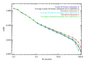
Figure 18: $w(\theta)$’s from Landy Szalay, Hamilton and standard estimator of the $700\ \rm deg^{-2}$ LRG sample. For comparison, the averaged $w(\theta)$’s from the 6 subfields (see text for more detail), are overplotted as measured from each estimator. Landy $\&$ Szalay and Hamilton estimators, give similar results for the average subfields and the full sample measurements, respectively. The standard estimator is more biased, at larger scales.

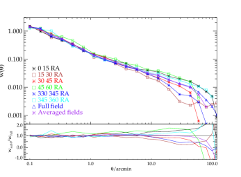
Figure 19: $w(\theta)$ results of the 6 equal size subfields ($15\times 2.5\rm deg^{2}$ each) across Stripe 82, the total area as estimated by using the Landy Szalay estimator and the averaged clustering signal from the 6 subfields. In the bottom panel are displayed the ratios of the $w(\theta)$ of each subfield compared to the total area.

$K$	LRGs $700\ deg^{-2}$
17.0-17.2	4894
17.2-17.4	11096
17.4-17.6	22490
17.6-17.8	38659
17.8-18.0	53680

Table 4: K-limited sub-samples used for auto-correlations in Fig. 20.

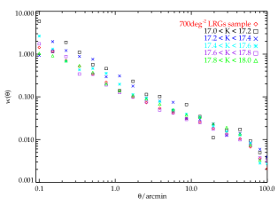
Figure 20: Auto-correlation functions from Landy-Szalay estimator for the $700\ deg^{-2}$ LRG K-limited sub-samples from Table 4. Total sample is overplotted for comparison.

7.2 Magnitude incompleteness

Another issue that we want to address is how the clustering signal can be affected by magnitude incompleteness. The $izK$ colour-selection used for the LRGs, applied up to the faintest limits of the SDSS-UKIDSS LAS surveys (see §2.1). To account for this, first we divide the $700\ \rm deg^{-2}$ LRG sample in 5 $K$ magnitude bins in the range $17<K<18$. The number of LRGs in each magnitude bin is shown in Table 4.

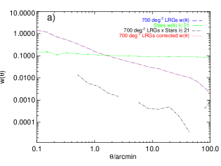
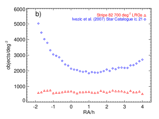
Figure 21: a) The observed $w(\theta)$ of Stripe 82 LRGs (blue dashed line), Stripe 82 star catalague of Ivezic et al. (2007) autocorrelation (green line) for $i\leq 21$, cross-correlations of the aforementioned LRGs-stars (black dashed-dot line) and the resulted corrected observed autocorrelation function following Ross et al. (2011). We see that there is no difference between the observed LRGs and the corrected $w(\theta)$’s, respectively. b) The number density of the stars up to $i=21$ from Ivezic et al. (2007) catalogue (blue diamonds) and the $700\rm\deg^{-2}$ LRG sample (red triangles) across the Stripe 82. There is a strong gradient in the star distribution towards one end of the Stripe 82 at $330\la RA\la 340$deg or $-2\la RA\la-1$hr in the abscissa notation. But when we excluded this area from the star-LRG cross-correlation, there was no change in the large-scale $w(\theta)$ signal.

Figure 22: The projected number density of Stripe 82 LRGs as a function of the potential observable systematics: stellar density ($n_{star}$), Galactic extinction ($A_{k}$) in the K-band, the K-band seeing ($see_{K}$), K-band background median sky flux in counts per pixel and the airmass (air). The errors are the standard deviation of the measurements within each bin.

Measurements of the angular correlation function from each $K$-bin are shown in Fig. 20, where measurement uncertainties are not shown as we are mostly interested in the shape of the $w(\theta)$ in the linear regime. The clustering signal from the $K$-magnitude bins compared to the full sample do not show any significant difference at large scales and follow the full sample $w(\theta)$ shape. At smaller scales we see that the clustering from the brighter samples is higher than for the fainter samples, as expected.

The final tests of the magnitude incompleteness check are via the use of brighter colours in the $zK$ selection. We therefore selected on the basis of brighter magnitudes down to $z\leq 21.2$ and $K\leq 17.2$, in various combinations and re-measured the angular correlation function. Even with these bright cuts, we did not see any change in the excess at large scales.

7.3 Observational parameters

The final test to identify a potential observational systematic effect follows the approach described by Ross et al. (2011), referring primarily to the area effectively masked by stars with magnitudes similar to the galaxies in the field. We cross-correlated the $700\ deg^{-2}$ LRG sample with the Stripe 82 star catalogue from Ivezić et al. (2007), in 4 magnitude bins, $i<19.5,20,20.5,21$. From the measured autocorrelation function of stars and the cross-correlation function of stars with LRGs we computed the effect of stellar masking on the LRG correlation function using their equations (28) and (29). We show these results in Fig. 21a.

The cross correlation results show a very small anticorrelation between LRGs and stars for the $i=19.5$ and $20.5$ bins. A possible explanation for this anticorrelation might be related to the fact that we see an increase in the star number density between $330\leq RA\leq 340$ $deg^{0}$ (see Fig. 21b). Next, we calculate the expected $w(\theta)$, as defined in Eq. 29 of Ross et al. (2011). In all cases, there was little difference in the expected and observed $w(\theta)$ of the $700\ \rm deg^{-2}$ LRG sample. We conclude that the effect of stellar masking is essentially negligible, less than 1% of the clustering signal at $\theta\approx 90^{\prime}$

There are other sources of possible systematics as well as star masking. Ross et al. (2011) also checked observational parameters such as galactic extinction, sky background, seeing and airmass using the cross-correlation technique. The Stripe 82 LRG sample is K-limited. Hence, we explore if the above observed parameters from the UKIDSS LAS K-band could be sources of systematic errors at large scales. Fig. 22 displays the number density of Stripe 82 LRGs and how it is related with each potential observational systematic (stars are from Ivezić et al. 2007). From Fig. 22 we see a sharp decrease in the number of LRGs with high galactic extinction and poor seeing. The airmass fluctuations are also large compared to the error bars. The majority of the LRGs lie within the first few bins of galactic extinction, seeing and airmass in Fig. 22, but the LRGs in the rest of the bins with higher values could introduce systematics in the clustering signal.

Ho et al. (2012) present a method to identify which combination of the observed parameters could have the biggest effect on the clustering measurements. The authors in this work expressed the linear relationship between the potential observational systematic and its effect on the observed overdensity of galaxies, through the $\epsilon$ factor. In Fig. 23a we show the $\epsilon_{i}$ parameters for each of the the observational parameters. The Ross et al. (2011) cross-correlation correction technique requires that $\epsilon$ be constant, so we use the best-fitting constant value of $\epsilon$ as calculated with the lowest chi-square fits from field-to-field errors. We find that the biggest correction in the angular correlation function is for the combined seeing, airmass and galactic extinction observational parameters (see Eq. 29 of Ross et al.). Also, a slightly smaller correction has been found for stars, sky background and galactic extinction. In Fig. 23b we show the original uncorrected $w(\theta)$ for the Stripe 82 LRGs, the $w(\theta)$ after applying the combined correction for the seeing, airmass and galactic extinction. In the same figure, for comparison we plot the best-fit $\Lambda\rm CDM$ model as displayed in Fig. 14. So far this correction in our $w(\theta)$ results is the most important. But still as we can see from Fig. 23b, at the range $20-80^{\prime}$, the amplitude of the angular correlation function does not show the expected behaviour of the standard model. We have checked for the most common sources of systematics in the literature. Our data could still be affected by hidden artefacts, a case that future studies might be able to identify, but for the moment we will take the corrected result in Fig. 23b as our best estimate. Note that the HOD fits of §5.4 were only done up to $\theta\leq 60^{\prime}$ where there is little change in the form of our $w(\theta)$ result.

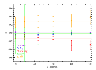
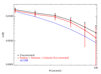
Figure 23: a) (upper) Similar to Ross et al. 2011 we plot $\epsilon$, the linear factor between the potential observational systematic and its effect on the observed overdensity of galaxies for stars (purple diamond), galactic extinction (blue diamond), seeing (red squares), sky background (green diamond) and airmass (orange triangle). The solid lines are the best-fitting constant value of $\epsilon$ for each systematic. b) (lower) The $w(\theta)$ measurement of the Stripe 82 LRGs without any cross-correlation correction (black star) and $w(\theta)$ corrected for seeing, airmass and galactic extinction combined (red diamond). The best-fit $\Lambda\rm CDM$ model to the uncorrected measurement is plotted (blue line).

8 Test for Non-Gaussianity

One possible explanation for the flat slope seen at large scales is scale-dependent bias, although this is usually discussed more in the context of small-scale clustering. However, scale dependent bias at large scales has previously been invoked to explain the discrepancy between the APM $w(\theta)$ results and $\Omega_{m}=1$ CDM models (Bower et al., 1993); in this case the scale dependence was caused by ‘cooperative galaxy formation’.

Another possibility is that the LRG power spectrum may be closer to the primordial power spectrum at higher redshifts. But we have seen that the Stripe 82 clustering result are not in line with the standard $\Lambda$CDM model. These correlation function results are better fitted by a model with $\Omega_{m}=0.2$ rather than $\Omega_{m}=0.27$ (see Fig. 14), useful at least as an illustration of the size of the LRG clustering excess.

The third possibility is that the $z\approx 1$ LRG power spectrum may be better explained by scale-dependent bias at large scales due to primordial non-Gaussianity in the density fluctuations. The primordial non-Gaussianity of the local type is parameterised by $f_{\rm NL}^{\rm local}$ (see Bartolo et al., 2004, for a review) and is expected to contribute a $1/k^{2}$ term to the power spectrum and evolves as $\approx 1+z$ (see Eq. 42). It is therefore best seen at large-scales and high redshifts. Fig. 1 of Xia et al. (2010) shows the potential effect of non-Gaussianity on the biased clustering of radio sources with a similar redshift to the LRGs discussed here. It can be seen that the non-Gaussianity causes a strong positive tail to the correlation function for $\theta>$ a few degrees.

Xia et al. (2010), following Blake & Wall (2002), found that the NVSS survey ACF showed a strong positive tail suggesting that $f_{NL}^{\rm local}=62\pm 27$. Xia et al. (2011) also inspected the angular correlation function of the DR6 $1\times 10^{6}$ QSO sample and found similar results to the radio sources with again an extended correlation function being seen implying similar values of $f_{\rm NL}$ (hereafter we shall use just $f_{\rm NL}$ to denote $f_{\rm NL}^{\rm local}$) as for the radio sources. This led to only slightly weaker constraints than for the radio sources in terms of the value of $f_{\rm NL}$.

Sawangwit et al. (2011) measured the combined angular correlation function of LRGs at $z\approx 0.35,0.55,0.68$ and found that although the results were in agreement with $\Lambda$CDM at scales $<100\rm h^{-1}$Mpc, at larger scales there was a possible excess, although this could still be due to systematics.

We then proceeded to follow Xia et al. and fit $f_{\rm NL}$ models. We use their relation between the non-Gaussian and Gaussian biases ($b_{NG}$ and $b_{G}$)

$$b_{\rm NG}(z)-b_{\rm G}(z)\simeq 2(b_{\rm G}(z)-1)f_{\rm NL}\delta_{\rm ec}(z)\alpha_{\rm M}(k)~{}.$$ (42)

Here $\delta_{\rm ec}(z)$ is the critical density for ellipsoidal collapse and $\alpha_{\rm M}(k)\propto 1/k^{2}$ contains the scale and halo mass dependence (see Xia et al. for more details.)

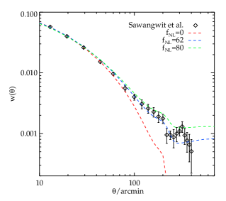
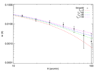
Figure 24: a) (upper) The combined correlation function of Sawangwit et al (2011) for the $z=0.35$, $z=0.55$ and $z=0.68$ LRG samples, compared to a standard LCDM model ($f_{nl}=0$) and models with increasing degrees of primordial non-Gaussianity ($f_{nl}=62,80$). b) (lower) The Stripe-82 $z\approx 1$ LRG correlation function compared to a standard LCDM model ($f_{nl}=0$) and models with increasing degrees of primordial non-Gaussianity ($f_{nl}=62,80,100$).

We first applied this relation to the case of the NVSS radio sources at $z\approx 0.7$. We found that adding the $1/k^{2}$ term to the standard cosmology $P(k)$ caused it to diverge and so we had to apply a large-scale cut-off, so that for $k<k_{0}$ then $P(k)=0$. This is clearly a source of uncertainty in fitting for $f_{\rm NL}$. Nevertheless, we found that for $k_{0}=10^{-6}$, we could reproduce the results of Xia et al. (2010).

We then applied the same technique and cut-off to the combined $AA\Omega$ LRG and the Stripe 82 LRG $w(\theta)$’s (after applying the combined correction for seeing, airmass and galactic extinction as estimated in § 7.3). We first took the value of $b_{G}=2.08$ from the halo model fits of Sawangwit et al. (2011) and fitted for $f_{NL}$. The result is shown in Fig. 24a. We find that for $AA\Omega$ LRGs, the results for $f_{NL}$ are reasonably compatible with those from the NVSS catalogue with values of $f_{\rm NL}=60-80$ giving a better fit to the data in the range $1.5<\theta<6.5$deg.

The prediction from non-Gaussianity is that the large scale slope will further flatten with redshift. We therefore compared the Stripe 82 LRGs to models with the same $f_{\rm NL}$ values and find no inconsistency (see Fig. 24b). Clearly the errors at the largest scales are more significant for the Stripe 82 data than for the $AA\Omega$ LRGs or the NVSS radio sources. However, the predicted flattening of the Stripe 82 correlation function at $\theta\approx 1$deg makes the non-Gaussian models more consistent with the data in this smaller angular range than the $f_{\rm NL}=0$ model. At larger scales the errors are larger and the data is therefore more in agreement with the standard model.

Figure 25: The minimum $\chi^{2}$ is 5.5 over 11 d.o.f and the best-fit parameters are $f_{\rm NL}=90\pm 30$ $(1\sigma)$ and $M_{min}=1.26\pm 0.22\times 10^{13}\rm h^{-1}M_{\odot}$. The best-fit $M_{min}$ here is lower than the full HOD fit assuming $f_{NL}=0$ at $2.2\times 10^{13}\rm h^{-1}M_{\odot}$.

Fig.  25 shows the effect of jointly fitting $f_{NL}$ on the minimum halo mass, $M_{min}$, in the HOD model. The best fit model now gives $M_{min}=(1.26\pm 0.22)\times 10^{13}h^{-1}M_{\odot}$ and $f_{NL}=90\pm 30$, lower than then the $M_{min}=2.2\times 10^{13}h^{-1}M_{\odot}$ value when $f_{nl}=0$ is assumed in the full HOD fit.

We should say that rather than detections of non-Gaussianity, the present $AA\Omega$ and Stripe 82 LRG results should be more regarded as upper limits on non-Gaussianity. Large-scale angular correlation function results are still susceptible to large-scale gradients and even though there is no direct evidence for these in the $AA\Omega$ or Stripe 82 samples, there is still the possibility that these exist in the data. On the other hand, the classic test for the reality of a correlation function feature is that it scales correctly with depth and at least the SDSS and Stripe 82 LRG correlation functions in Figs. 24a,b look like they do so. It will be interesting to see if as QSO surveys (Sawangwit et al., 2012) and $z\approx 3$ LBG surveys (Bielby et al., 2012) grow, whether the correlation functions at higher redshift also show an increased slope flattening as predicted for the non-Gaussian models.

The other uncertainty that has arisen is in the non-Gaussian model itself where we have found that there is a rather strong dependence on a small-scale cut-off, $k_{0}$. Other authors have made some reference to this problem but only implicitly. It will be interesting to see if more accurate models for non-Gaussianity can numerically predict this cut-off from first principles.

9 Summary and conclusions

We have measured $w(\theta)$ for $\approx 130\,000$ colour selected galaxies in Stripe 82 exploiting SDSS DR7 $i+z$ bands and UKIDSS LAS $K$ photometry. We used the cross-correlation technique of Newman (2008) to establish that the average redshift of the LRGs is $z\approx 1$. This sample therefore probes higher redshifts than the previous SDSS LRG samples of Sawangwit et al. (2011). We have established that a sample with sky density $\approx 700$deg^-2 has a comparable space density to the $z\approx 0.68$ $AA\Omega$ LRG sample of Sawangwit et al. (2011). However, this is only an approximate correspondence which makes evolutionary comparisons between the redshifts more tricky. What is clear is that the $z\approx 1$ LRGs generally have a relatively high clustering amplitude. Compared to the $AA\Omega$ LRG $w(\theta)$ scaled to the depth of the Stripe 82 LRGs, the Stripe 82 $w(\theta)$ is higher at all scales, even those below $<1\ \rm h^{-1}$Mpc. Thus at intermediate scales, the $z\approx 1$ LRGs are not only more clustered than predicted by the long-lived evolutionary model, they are also more clustered than the comoving model. At small separations ($\la 1\ \rm h^{-1}$Mpc) the correlation function amplitude is again somewhat higher than the $AA\Omega$ results scaled by the previously preferred stable clustering model. The Stripe 82 $w(\theta)$ also shows a very flat slope at large scales which means that the $\Lambda\rm$CDM linear model has become a poorer fit than at lower redshift.

Partly to look for an explanation for the flat large-scale slope, we then fitted a HOD model to the Stripe 82 $w(\theta)$. The best fit parameters were $M_{min}=2.19\pm 0.63\times 10^{13}\ \rm h^{-1}M_{\odot}$, $M_{1}=21.9\pm 5.6\times 10^{13}\ \rm h^{-1}M_{\odot}$, $b_{\rm lin}=2.81\pm 0.18$, $M_{\rm eff}=3.3\pm 0.6\times 10^{13}\ \rm h^{-1}M_{\odot}$, $F_{\rm sat}=3.17\pm 0.08\%$ and $n_{\rm g}=0.8\pm 0.3\times 10^{-4}\ \rm h^{3}Mpc^{-3}$. The high amplitude of the correlation function clearly pushes the halo masses up and the space densities down. The lowest chi-square fits were found when large scales were excluded but the reduced chi-squares were still in the range 2.3-3.6. This is actually an improvement over the lower redshift samples but this is certainly due to the larger errors on the Stripe 82 data. We conclude that it is not possible to find an explanation for the flat slope in the Stripe 82 $w(\theta)$ on the basis of the HOD model.

We also then studied the evolution of the HOD between $z=1$ and $z=0.35$. Similar to Sawangwit et al. (2011), we concluded that a pure passive model with a low merger rate might produce too steep a $w(\theta)$ slope at small scales ($<1\ \rm h^{-1}Mpc$). In this case, we have already noted that the small scale amplitude may also be too high for a passive model with stable clustering.

We have looked for an explanation of the flat slope in terms of systematics by cross correlating the Stripe 82 LRG sample with stellar density, airmass, seeing, sky background and galactic extinction and used the method of Ross et al. (2011) to correct our $w(\theta)$. Even the combined correction for seeing, airmass and galactic extinction only produced a small change in $w(\theta)$ at large scales.

We conclude that the high amplitude and flat slope of the Stripe 82 LRGs $w(\theta)$ may have a significant contributions from the uncertainty in the comparison between $AA\Omega$ and Stripe 82 LRG luminosities. However, this leaves a similar contribution from a new and unknown source. We have discussed large-scale, primordial, non-Gaussianity as one possibility for the source of this large-scale excess. We have suggested that the evidence from the $AA\Omega$ sample itself for an excess at even larger scales may fit in with the behaviour expected from non-Gaussianity over this redshift range. In this case we returned to the fitting of halo masses including the non-Gaussian component and found that the best fit $M_{min}$ decreased from $2.2\times 10^{13}$M_⊙ to $1.3\times 10^{13}$M_⊙. More importantly, if the Stripe 82 large-scale $w(\theta)$ excess proves reliable and not due to systematics, then we have made a significant detection of non-Gaussianity in the $z\approx 1$ LRG distribution with an estimated local non-Gaussianity parameter estimate of $f_{\rm NL}^{\rm local}=90\pm 30$. This represents a $3\sigma$ detection at a level comparable to the present upper limit from WMAP CMB measurements of $f_{\rm NL}^{\rm local}=32\pm 21$ (Komatsu, 2010).

References

- Abazajian et al. (2009) Abazajian K. N., et al., 2009, ApJS, 182, 543
- Bartolo et al. (2004) Bartolo, N., Komatsu, E., Matarrese, S., & Riotto, A. 2004, PhR, 402, 103
- Baugh (2006) Baugh C. M., 2006, RPPh, 69, 3101
- Berlind & Weinberg (2002) Berlind A. A., Weinberg D. H., 2002, ApJ, 575, 587
- Bielby et al. (2012) Bielby R., et al., 2012, arXiv, arXiv:1204.3635
- Blake & Wall (2002) Blake C., Wall J., 2002, MNRAS, 337, 993
- Blake, Collister, & Lahav (2008) Blake C., Collister A., Lahav O., 2008, MNRAS, 385, 1257
- Bower et al. (1993) Bower R. G., Coles P., Frenk C. S., White S. D. M., 1993, ApJ, 405, 403
- Brown et al. (2008) Brown M. J. I., et al., 2008, ApJ, 682, 937
- Bruzual & Charlot (2003) Bruzual G., Charlot S., 2003, MNRAS, 344, 1000
- Cannon et al. (2006) Cannon R., et al., 2006, MNRAS, 372, 425
- Collister et al. (2007) Collister A., et al., 2007, MNRAS, 375, 68
- Cooray & Sheth (2002) Cooray A., Sheth R., 2002, PhR, 372, 1
- Crocce et al. (2011) Crocce M., Gaztañaga E., Cabré A., Carnero A., Sánchez E., 2011, MNRAS, 417, 2577
- Davis et al. (2003) Davis M., et al., 2003, SPIE, 4834, 161
- Davis et al. (2007) Davis M., et al., 2007, ApJ, 660, L1
- Eisenstein et al. (2001) Eisenstein D. J., et al., 2001, AJ, 122, 2267
- Eisenstein et al. (2003) Eisenstein D. J., et al., 2003, ApJ, 585, 694
- Fry (1996) Fry J. N., 1996, ApJ, 461, L65
- Gonzalez-Perez et al. (2011) Gonzalez-Perez V., Baugh C. M., Lacey C. G., Kim J.-W., 2011, MNRAS, 417, 517
- Groth & Peebles (1977) Groth E. J., Peebles P. J. E., 1977, ApJ, 217, 385
- Guo, Zehavi, & Zheng (2011) Guo H., Zehavi I., Zheng Z., 2011, arXiv, arXiv:1111.6598
- Hamilton (1993) Hamilton A. J. S., 1993, ApJ, 417, 19
- Ho et al. (2012) Ho S., et al., 2012, arXiv, arXiv:1201.2137
- Ivezić et al. (2007) Ivezić Ž., et al., 2007, AJ, 134, 973
- Jing, Mo, & Boerner (1998) Jing Y. P., Mo H. J., Boerner G., 1998, ApJ, 494, 1
- Kim et al. (2011) Kim J.-W., Edge A. C., Wake D. A., Stott J. P., 2011, MNRAS, 410, 24
- Komatsu (2010) Komatsu E., 2010, CQGra, 27, 124010
- Kravtsov et al. (2004) Kravtsov A. V., Berlind A. A., Wechsler R. H., Klypin A. A., Gottlöber S., Allgood B., Primack J. R., 2004, ApJ, 609, 35
- Lacey & Cole (1993) Lacey C., Cole S., 1993, MNRAS, 262, 627
- Landy & Szalay (1993) Landy S. D., Szalay A. S., 1993, ApJ, 412, 64
- Lawrence et al. (2007) Lawrence A., et al., 2007, MNRAS, 379, 1599
- Lewis, Challinor, & Lasenby (2000) Lewis A., Challinor A., Lasenby A., 2000, ApJ, 538, 473
- Limber (1953) Limber D. N., 1953, ApJ, 117, 134
- Loh & Strauss (2006) Loh Y.-S., Strauss M. A., 2006, MNRAS, 366, 373
- Lupton et al. (2001) Lupton R., Gunn J. E., Ivezić Z., Knapp G. R., Kent S., Yasuda N., 2001, ASPC, 238, 269
- Ma & Fry (2000) Ma C.-P., Fry J. N., 2000, ApJ, 543, 503
- Masjedi et al. (2006) Masjedi M., et al., 2006, ApJ, 644, 54
- Moore et al. (2001) Moore A. W., et al., 2001, misk.conf, 71
- Myers et al. (2007) Myers A. D., Brunner R. J., Nichol R. C., Richards G. T., Schneider D. P., Bahcall N. A., 2007, ApJ, 658, 85
- Newman (2008) Newman J. A., 2008, ApJ, 684, 88
- Navarro, Frenk, & White (1997) Navarro J. F., Frenk C. S., White S. D. M., 1997, ApJ, 490, 493
- Norberg et al. (2009) Norberg P., Baugh C. M., Gaztañaga E., Croton D. J., 2009, MNRAS, 396, 19
- Padmanabhan et al. (2007) Padmanabhan N., et al., 2007, MNRAS, 378, 852
- Papageorgiou et al. (2012) Papageorgiou A., Plionis M., Basilakos S., Ragone-Figueroa C., 2012, MNRAS, 422, 106
- Peacock & Smith (2000) Peacock J. A., Smith R. E., 2000, MNRAS, 318, 1144
- Peebles (1980) Peebles P. J. E., 1980, lssu.book,
- Richards et al. (2009) Richards G. T., et al., 2009, ApJS, 180, 67
- Roche & Eales (1999) Roche N., Eales S. A., 1999, MNRAS, 307, 703
- Ross, Brunner, & Myers (2008) Ross A. J., Brunner R. J., Myers A. D., 2008, ApJ, 682, 737
- Ross & Brunner (2009) Ross A. J., Brunner R. J., 2009, MNRAS, 399, 878
- Ross, Percival, & Brunner (2010) Ross A. J., Percival W. J., Brunner R. J., 2010, MNRAS, 407, 420
- Ross et al. (2011) Ross A. J., et al., 2011, MNRAS, 417, 1350
- Ross et al. (2007) Ross N. P., et al., 2007, MNRAS, 381, 573
- Ross et al. (2008) Ross N. P., Shanks T., Cannon R. D., Wake D. A., Sharp R. G., Croom S. M., Peacock J. A., 2008, MNRAS, 387, 1323
- Sawangwit et al. (2011) Sawangwit U., Shanks T., Abdalla F. B., Cannon R. D., Croom S. M., Edge A. C., Ross N. P., Wake D. A., 2011, MNRAS, 416, 3033
- Sawangwit et al. (2012) Sawangwit, U., Shanks, T., Croom, S. M., et al. 2012, MNRAS, 420, 1916
- Schlegel, Finkbeiner, & Davis (1998) Schlegel D. J., Finkbeiner D. P., Davis M., 1998, ApJ, 500, 525
- Schneider et al. (2010) Schneider D. P., et al., 2010, AJ, 139, 2360
- Scoccimarro et al. (2001) Scoccimarro R., Sheth R. K., Hui L., Jain B., 2001, ApJ, 546, 20
- Scranton et al. (2002) Scranton R., et al., 2002, ApJ, 579, 48
- Seljak (2000) Seljak U., 2000, MNRAS, 318, 203
- Seo, Eisenstein, & Zehavi (2008) Seo H.-J., Eisenstein D. J., Zehavi I., 2008, ApJ, 681, 998
- Shanks et al. (1983) Shanks T., Bean A. J., Ellis R. S., Fong R., Efstathiou G., Peterson B. A., 1983, ApJ, 274, 529
- Sheth & Lemson (1999) Sheth R. K., Lemson G., 1999, MNRAS, 304, 767
- Sheth, Mo, & Tormen (2001) Sheth R. K., Mo H. J., Tormen G., 2001, MNRAS, 323, 1
- Sheth & Tormen (2002) Sheth R. K., Tormen G., 2002, MNRAS, 329, 61
- Skibba & Sheth (2009) Skibba R. A., Sheth R. K., 2009, MNRAS, 392, 1080
- Smith et al. (2003) Smith R. E., et al., 2003, MNRAS, 341, 1311
- Tinker et al. (2005) Tinker J. L., Weinberg D. H., Zheng Z., Zehavi I., 2005, ApJ, 631, 41
- Wake et al. (2006) Wake D. A., et al., 2006, MNRAS, 372, 537
- Wake et al. (2008) Wake D. A., Croom S. M., Sadler E. M., Johnston H. M., 2008, MNRAS, 391, 1674
- Warren et al. (2007) Warren S. J., et al., 2007, MNRAS, 375, 213
- White et al. (2007) White M., Zheng Z., Brown M. J. I., Dey A., Jannuzi B. T., 2007, ApJ, 655, L69
- Xia et al. (2010) Xia J.-Q., Viel M., Baccigalupi C., De Zotti G., Matarrese S., Verde L., 2010, ApJ, 717, L17
- Xia et al. (2011) Xia J.-Q., Baccigalupi C., Matarrese S., Verde L., Viel M., 2011, JCAP, 8, 33
- Zehavi et al. (2005a) Zehavi I., et al., 2005a, ApJ, 621, 22
- Zehavi et al. (2005b) Zehavi I., et al., 2005b, ApJ, 630, 1
- Zheng et al. (2009) Zheng Z., Zehavi I., Eisenstein D. J., Weinberg D. H., Jing Y. P., 2009, ApJ, 707, 554