Physical properties of interstellar filaments

We analyze the physical parameters of interstellar filaments that we describe by an idealized model of isothermal self-gravitating infinite cylinder in pressure equilibrium with the ambient medium. Their gravitational state is characterized by the ratio $f_{\rm cyl}$ of their mass line density to the maximum possible value for a cylinder in a vacuum. Equilibrium solutions exist only for $f_{\rm cyl}<1$. This ratio is used in providing analytical expressions for the central density, the radius, the profile of the column density, the column density through the cloud centre, and the fwhm. The dependence of the physical properties on external pressure and temperature is discussed and directly compared to the case of pressure-confined isothermal self-gravitating spheres. Comparison with recent observations of the fwhm and the central column density $N_{\rm H}(0)$ show good agreement and suggest a filament temperature of $\sim 10\leavevmode\nobreak\ {\rm K}$ and an external pressure $p_{\rm ext}/k$ in the range $1.5\times 10^{4}\leavevmode\nobreak\ {\rm K\leavevmode\nobreak\ cm}^{-3}$ to $5\times 10^{4}\leavevmode\nobreak\ {\rm K\leavevmode\nobreak\ cm^{-3}}$. Stability considerations indicate that interstellar filaments become increasingly gravitationally unstable with mass line ratio $f_{\rm cyl}$ approaching unity. For intermediate $f_{\rm cyl}>0.5$ the instabilities should promote core formation through compression, with a separation of about five times the fwhm. We discuss the nature of filaments with high mass line densities and their relevance to gravitational fragmentation and star formation.

1 Introduction

Filamentary structures are an ubiquitous phenomenon in the interstellar medium. Thanks to the high angular resolution and signal to noise of dust imaging with the Herschel Space Observatory, it is now possible to quantify the basic empirical properties of filaments. Filaments have been imaged in the submillimetre in exquisite detail in non star-forming such as Polaris (Men’shchikov et al. 2010; Miville-Deschênes et al. 2010), in molecular regions with low-mass star formation such as Aquila and IC 5146 (André et al. 2010; Arzoumanian et al. 2011; Men’shchikov et al. 2010), and in higher-mass regions including Vela C and the Rosette molecular cloud (Hill et al. 2011; Schneider et al. 2012). At least in the low-mass star forming regions and in Polaris , the characteristic filament sizes are about 0.1 pc (Arzoumanian et al. 2011).

Clear evidence for star formation seems to be related to cloud structures with a typical extinction larger then $A_{V}\approx 7\leavevmode\nobreak\ {\rm mag}$ (Onishi et al. 1998; Johnstone et al. 2004; André et al. 2010), which corresponds to a column density $N_{\rm H}$ about $0.6\times 10^{22}$ cm^-2 (see comments in Appendix A). Furthermore, the Herschel studies show that high column densities are typically associated with filaments and, finally, that cold dense clouds called “prestellar cores” possibly related to the very early stages of the star formation (Könyves et al. 2010), are observed mainly along filaments (André et al. 2010; Men’shchikov et al. 2010; Arzoumanian et al. 2011). Empirically, it is found that filaments that are star forming are characterized by not only a higher central column density but also a higher mass per unit length (André et al. 2010; Arzoumanian et al. 2011). It is argued that the cores are possibly created out of the elongated structures through gravitational instabilities (Schneider & Elmegreen 1979; Gaida et al. 1984; Hanawa et al. 1993; Curry 2000; André et al. 2010; Men’shchikov et al. 2010).

It is important to develop a physical model for the filaments so that the new measurements can be exploited. That is the goal of this paper. The basic model that we explore is an isothermal cylinder confined at a finite boundary $r_{\rm cyl}$ by an external pressure $p_{\rm ext}$ provided by an ambient or embedding medium. This is certainly more realistic than an isothermal cylinder in vacuum, whose properties (such as the radial profile) are not surprisingly in disagreement with observations (e.g., Men’shchikov et al. 2010; Arzoumanian et al. 2011). Even these pressure-confined models are unlikely to describe what is a very complex interstellar medium where the origin of the filamentary structures is still a mystery, but the models can serve the same role in developing our understanding that has been played by the spherically-symmetric analog, the Bonnor-Ebert sphere (Ebert 1955; Bonnor 1956; Nagasawa 1987; Inutsuka & Miyama 1992, 1997; Curry & McKee 2000; Fiege & Pudritz 2000; Kandori et al. 2005; Fischera & Dopita 2008). Furthermore, we find that the models do actually provide a consistent description of the sizes and column densities recently reported for filaments and some insight into the instabilities relating to filaments.

We analyze systematically the physical properties of pressure-confined filaments, comparing and contrasting these results with the corresponding properties for spheres. We develop analytical solutions for several observables. Parts of the results, on which we build, can be found in earlier work on the spectral energy distribution of interstellar clouds (Fischera & Dopita 2008 – paper I) and on the spectral energy distribution of condensed cores embedded in pressurized elongated or spherical clouds (Fischera 2011 – paper II).

Our paper is organized as follows. The physical model is presented in Section 2, from which properties are derived in Section 3. Observed properties corresponding to size and column density are compared with the model in Section 4 with remarkable agreement. Structure formation due to instability of the filaments is discussed in Section 5. It seems plausible that dominant protostellar cores arranged along filaments could arise from a “compressive instability” (Nagasawa 1987) in high column density filaments. Some other instabilities seem less relevant. A summary and discussion is provided in Section 6. Several appendices deal with the astronomical context and details of some calculations.

2 Physical model

We assume that the filaments can be described by a model of isothermal self-gravitating infinitely long cylinders. For the isothermal gas, the relationship between gas pressure $p$ and gas density $\rho$ is

$$K=p/\rho=Tk/(\mu m_{\rm H}),$$ (1)

where $k$ is the Boltzmann constant, $\mu$ the mean molecular weight (2.36 for a molecular cloud with cosmic abundances), and $m_{\rm H}$ the mass of the hydrogen atom; the isothermal temperature $T$ is considered to be an effective value related to both the thermal and the turbulent motion of the gas (see Appendix A.4). If the effective temperature is equal to the thermal or kinetic temperature then $K=c_{\rm s}^{2}$, the square of the sound speed. Furthermore, as discussed in the introduction, the clouds are assumed to be in pressure equilibrium with the surrounding medium of pressure $p_{\rm ext}$. This does not imply that the external medium is isothermal or at the same temperature; it is simply a boundary condition.

2.1 Cloud profile

Isothermal self-gravitating infinitely long cylinders have a well-known density or pressure profile given by (see e.g. Stodólkiewicz (1963); Ostriker (1964))

$$\rho(r)=\frac{\rho_{c}}{(1+(r/\sqrt{8}r_{0})^{2}))^{2}},$$ (2)

where

$$r_{0}^{2}=K/(4\pi G\rho_{c}),$$ (3)

$\rho_{c}$ is the central density, and $G$ the gravitational constant. For pressure-confined clouds the profile terminates where the cloud pressure is equal to the external pressure $p_{\rm ext}$; this defines the cylinder radius $r_{\rm cyl}$. As in papers I and II, in the following we refer to the ratio $p_{\rm c}/p_{\rm ext}$ as the “overpressure.”

2.2 Mass line density

Analogous to the cloud mass in the case of spherical clouds we have in the case of cylinders the mass per cloud length (mass line density), given by

$$\frac{M}{l}(r_{\rm cyl}) = \int_{0}^{r_{\rm cyl}}{\rm d}r\,2\pi r\,\rho(r)$$ (4)

$$= \frac{2K}{G}\left\{1-\frac{1}{1+{r_{\rm cyl}}^{2}/(8r_{0}^{2})}\right\}.$$

In the limit $r_{\rm cyl}\gg\sqrt{8}r_{0}$ the mass per cloud lengths approaches asymptotically a maximum value given by

$$\left(\frac{M}{l}\right)_{\rm max}=\frac{2K}{G}=16.4\,\left(\frac{T}{10\leavevmode\nobreak\ {\rm K}}\right)\,{\rm M}_{\odot}\leavevmode\nobreak\ {\rm pc}^{-1}.$$ (5)

For pressurized clouds this gravitational state corresponds to an infinite overpressure, but there is no dependence on $p_{\rm ext}$.

For comparison, in the case of an isothermal self-gravitating pressurized sphere, the maximum mass is identical to its critical mass, given by (see Appendix B)

$$M_{\rm sph,cr}\approx 4.191\frac{K^{2}}{\sqrt{4\pi G^{3}p_{\rm ext}}}.$$ (6)

This gravitational state is characterized by an overpressure $p_{\rm c}/p_{\rm ext}\approx 14.04$. As shown in paper II, a critical stable state is related to the maximum possible pressure that a sphere of given mass and $K$ (temperature) can produce at the cloud outskirts under compression. If the external pressure is increased slightly, the resulting equilibrium configuration is unstable to gravitational collapse, and so this is aptly called a “critical stable sphere”. The spherical clouds can be characterized as “subcritical” or “supercritical” depending on whether the overpressure is lower or higher than the value for a critical stable sphere. Note that for overpressures higher than 14.04, the mass of an equilibrium configuration is smaller than the critical mass. Thus we can also say that for given $p_{\rm ext}$ and $K$ the critical mass is the maximum mass for which an equilibrium solution exists.

Unlike $M_{\rm sph,cr}$, the maximum mass line density depends only linearly (compared to quadratically) on $K$ or cloud temperature and does not depend at all on the size of the external pressure confining the cloud. We discuss the basic consequences in Sect. 3.6 and Sect. 3.7.

There are no equilibrium solutions for cylinders or spheres with masses above the corresponding maximum values (McCrea 1957). They would collapse radially towards a line (spindle) or to a singular point, respectively. This has led to the terminology “supercritical mass” when $M>M_{\rm sph,cr}$, or “supercritical filament” when $M/l>(M/l)_{\rm max}$. The gravitational states considered in this paper are all equilibrium solutions. We prefer to reserve the term “supercritical” to describe the equilibrium states for spheres, as above, and note the fundamental difference that there are no such supercritical equilibrium states for cylinders (Sect. 3.6 ).

2.2.1 Mass fraction $f_{\rm cyl}$

A very useful quantity is the mass fraction

$$f_{\rm cyl}=(M/l)/(M/l)_{\rm max}\leq 1.$$ (7)

For cylinders we find directly from Eqs. 1 to 7 that the overpressure

$$p_{\rm c}/p_{\rm ext}=1/(1-f_{\rm cyl})^{2}.$$ (8)

We can therefore use $f_{\rm cyl}$ to characterize the gravitational state of the cylinders. This mass ratio therefore appears in the formulae below for the derived properties of cylinders in different gravitational states. Two instructive limits to consider are the case of high overpressure or $f_{\rm cyl}\rightarrow 1$, which we shall see corresponds to a narrow high column density filament with strong self-gravity, and the case of vanishing overpessure or $f_{\rm cyl}\rightarrow 0$, corresponding to a filament much more difficult to recognize or characterize. There is, however, no distinction between “pressure-confined” and “self-gravitating” cylinders, since both features are intrinsic to all equilibrium models.

This parallels the approach used in paper I where the gravitational state of pressurized spheres was described by the mass ratio $f_{\rm sph}=M/M_{\rm sph,cr}$ of the cloud mass relative to the mass of a critical stable sphere. While in paper I the physical parameters for spheres were discussed only for the physically stable regime with overpressures below the critical value 14.04, we consider here the whole physical range. This leads to the curious situation that for large overpressures above the critical value the gravitational state is described by $f_{\rm sph}<1$.

3 Derived properties

In the following we describe the physical properties of molecular cylinders and compare spheres for a given cloud temperature and external pressure. We adopt illustrative reference values for temperature and pressure. See Appendix A for further discussion. For the cold molecular clouds we adopt $K$ corresponding to 10 K ($c_{\rm s}=0.19$ km s^-1). For the external pressure we adopt $p_{\rm ext}/k=2\times 10^{4}\leavevmode\nobreak\ {\rm K\leavevmode\nobreak\ cm}^{-3}$, consistent with paper I and paper II.

3.1 Central density

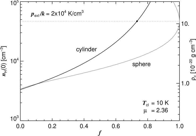
Figure 1: Central density of an isothermal self-gravitating molecular cylinder (black) and sphere (grey), for fixed values of the ambient pressure. $p_{\rm ext}/k=2\times 10^{4}\leavevmode\nobreak\ {\rm K\leavevmode\nobreak\ cm}^{-3}$ and cloud temperature $T=10\leavevmode\nobreak\ {\rm K}$. The dotted line is the value achieved by a critical stable sphere. This same central density (or overpressure) is reached in a cylinder with $f_{\rm cyl}=0.733$ (filled black circle).

For the central density we have from Eqs. 1 and 8

$$\rho_{\rm c}=\frac{p_{\rm ext}}{K(1-f_{\rm cyl})^{2}}.$$ (9)

The central number density $n_{\rm H}(r=0)\equiv n_{\rm H}(0)$ is obtained by evaluating

$$n_{\rm H}=\rho\left(\sum\frac{n_{i}}{n_{\rm H}}\mu_{i}m_{\rm H}\right)^{-1}\equiv\rho\,(\bar{\mu}m_{\rm H})^{-1},$$ (10)

where $n_{i}/n_{\rm H}$ is the relative abundance of element $i$ compared to H, and $\mu_{i}$ is its relative mass units of $m_{\rm H}$; on the right, the effective mass per H, $\bar{\mu}$, is 1.4 for cosmic abundances. Figure 1 shows these central values as a function of the mass fraction.

For a given temperature and external pressure the central density increases as $1/(1-f_{\rm cyl})^{2}$ and so in the limit $f_{\rm cyl}\rightarrow 1$ the density becomes infinite.

For a given mass fraction, the density in the cloud centre is proportional to $p_{\rm ext}\mu/T$. Cylinders have a higher overpressure or overdensity in the cloud centre compared to spheres (Fig. 1) for the same mass fraction, except in the case of small mass fractions ($f<\approx 0.15$). In cylinders the overpressure of 14.04 corresponding to critical stable spheres is achieved for a mass fraction of $f_{\rm cyl}\approx 0.733$.

3.2 Cloud radius

Solving Eq. 4 for $r_{\rm cl}$, using Eq. 9 and recasting Eq. 3 as

$$r_{0}=\frac{K}{\sqrt{4\pi Gp_{\rm ext}}}(1-f_{\rm cyl}),$$ (11)

provides

$$r_{\rm cyl}=\frac{\sqrt{8}K}{\sqrt{4\pi Gp_{\rm ext}}}\sqrt{\frac{1}{4}-\left(f_{\rm cyl}-\frac{1}{2}\right)^{2}}.$$ (12)

This along with the boundary radius of the pressure-confined sphere is plotted as $r_{\rm cl}$ in Figure 2 as a function of mass fraction.

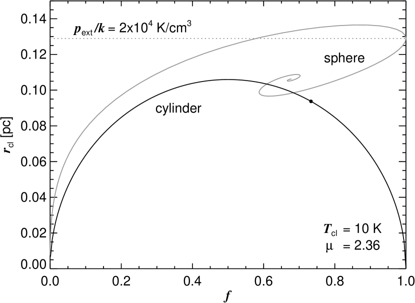
Figure 2: Like Fig. 1, but for the radius of an isothermal self-gravitating cylinder (black) and sphere (grey).

The size of the cloud for given mass fraction $f$ is proportional to $(T/\mu)/\sqrt{p_{\rm ext}}$. The radius for cylinders is symmetrical around $f=0.5$ where the cloud shows its maximum size. The filament grows in size through accretion of new material as long as the mass ratio $f_{\rm cyl}<0.5$. Further accretion will cause a shrinking of the filament. In the limit $f_{\rm cyl}\rightarrow 1$ (the mass-line density approaches the maximum value $2K/G$) the cylinder will become infinitely thin.

Spheres by contrast have a finite size at large mass ratios. As pointed out in paper I the spherical cloud has a maximum size at $f_{\rm sph}\approx 0.870$. Pushed above this value by accretion an isothermal cloud size shrinks to the size of a critical stable cloud. Supercritical stable spheres have smaller sizes still.

3.3 Radial profile of the pressure or density

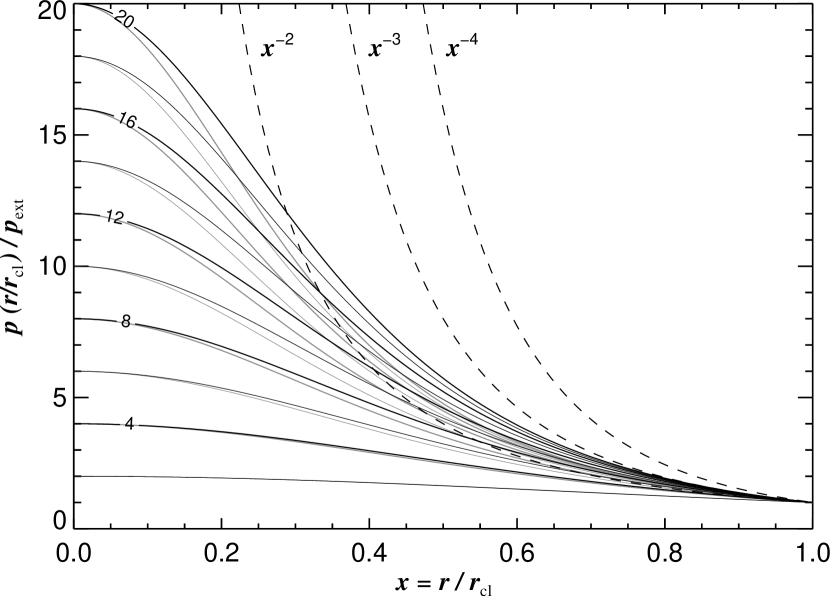
Figure 3: Pressure profiles of isothermal self-gravitating cylinders (black) and spheres (grey), for various overpressures $p_{\rm c}/p_{\rm ext}$ from 2 to 20. The dashed curves show density profiles for simple power laws normalized at the cloud boundary.

The radial dependence of pressure given by Eq. 2 is shown in Fig. 3 for various overpressures, which according to Eq. 9 are equivalent to $1/(1-f_{\rm cyl})^{2}$. For comparison, profiles are also shown for spheres for the same set of overpressures; in the central region of the cloud their density falls off more strongly towards larger radii.

In the limit of $r^{2}/(8r_{0}^{2})\gg 2$ the clouds show a steep density profile at the cloud edges with $\rho(r)\propto r^{-4}$. However, this property requires clouds with very high overpressures (large $f_{\rm cyl}$, close to the maximum possible mass-line density). n the outer half of the cylinders the density profiles for overpressures less than 20 are shallower than a $r^{-4}$ profile. For overpressures in the regime 6 to 12 the density profile at the outer half is more consistent with a $r^{-2}$-profile. Compared to spheres,

A useful characteristic size for describing properties of the cylinder is $r_{\rm cyl}$ for small $f_{\rm cyl}$ and $\sqrt{8}r_{0}$ for large $f_{\rm cyl}$.

3.4 Projection of the density profile

3.4.1 Column density profile

The column density at an impact parameter $x$ (in units of cloud radius $r_{\rm cl}$) is given by the integral

$$N_{\rm H}(x)=2\int\limits_{0}^{r_{\rm cyl}\sqrt{1-x^{2}}}\frac{n_{\rm H}(0)\,{\rm d}r}{(1+x^{2}r_{\rm cyl}^{2}/8r_{0}^{2}+r^{2}/8r_{0}^{2})^{2}}.$$ (13)

The integral evaluates to:

$$N_{\rm H}(x)=n_{\rm H}(0)\sqrt{8}\frac{r_{0}}{c}\Big{\{}\frac{u}{u^{2}+c}+\frac{1}{\sqrt{c}}\arctan{\frac{u}{\sqrt{c}}}\Big{\}},$$ (14)

with $c=1+x^{2}r_{\rm cyl}^{2}/8r_{0}^{2}$ and $u=\sqrt{1-x^{2}}\,r_{\rm cyl}/(\sqrt{8}r_{0})$. Using the replacement $r_{\rm cyl}^{2}/8r_{0}^{2}=f_{\rm cyl}/(1-f_{\rm cyl})$ it is straightforward to show that the column density profile for given $f_{\rm cyl}$ is given by:

$$N_{\rm H}(x) = \sqrt{\frac{p_{\rm ext}}{4\pi G}}\frac{\sqrt{8}}{1-f_{\rm cyl}}(\bar{\mu}m_{\rm H})^{-1}$$ (15)

$$\times\frac{1-f_{\rm cyl}}{1-f_{\rm cyl}+x^{2}f_{\rm cyl}}\Bigg{\{}\sqrt{f_{\rm cyl}(1-f_{\rm cyl})(1-x^{2})}$$

$$+\sqrt{\frac{1-f_{\rm cyl}}{1-f_{\rm cyl}(1-x^{2})}}$$

$$\times\arctan{\sqrt{\frac{f_{\rm cyl}(1-x^{2})}{1-f_{\rm cyl}(1-x^{2})}}}\Bigg{\}}.$$

The profile shape is solely determined by the mass fraction $f_{\rm cyl}$. The amplitude of the profile with fixed $f_{\rm cyl}$ is proportional to $\sqrt{p_{\rm ext}}$ and is independent of the cloud temperature.

In the limit $f_{\rm cyl}\rightarrow 1$ the profile for $x\ll 1$ can be approximated by:

$$N_{\rm H}(x) \approx \sqrt{\frac{p_{\rm ext}}{4\pi G}}\frac{\sqrt{8}}{1-f_{\rm cyl}}(\bar{\mu}m_{\rm H})^{-1}$$ (16)

$$\times\left(\frac{1-f_{\rm cyl}}{1-f_{\rm cyl}(1-x^{2})}\right)^{3/2}\frac{\pi}{2}.$$

In the limit of low $f_{\rm cyl}$

$$N_{\rm H}(x)\approx(p_{\rm ext}/K)(\bar{\mu}m_{\rm H})^{-1}2\sqrt{1-x^{2}}\,r_{\rm cyl},$$ (17)

as for a uniform-density cylinder.

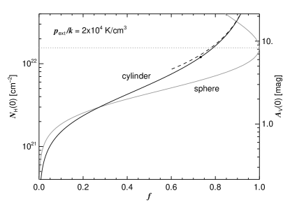
Figure 4: Like Fig. 1, but for the central column density (left panel) and mean column density (right panel) through an isothermal self-gravitating cylinder (black) and sphere (grey), as a function of mass fraction $f$. The dashed line in the left-hand plot is the approximation given in Eq. 19. The dashed lines in the right-hand plot echo the central column densities from the left-hand plot for comparison. The horizontal dotted lines give the values achieved by a critical stable sphere. The values for a cylinder with that overpressure, mass fraction 0.733, are shown as filled black circles.

3.4.2 Central column density

An important characteristic of self-gravitating clouds is the column density through the cloud centre, $N_{\rm H}(0)$, which for cylinders is a trivial solution of Eq. 15 for $x=0$:

$$N_{\rm H}(0) = \sqrt{\frac{p_{\rm ext}}{4\pi G}}\frac{\sqrt{8}}{1-f_{\rm cyl}}(\bar{\mu}m_{\rm H})^{-1}$$ (18)

$$\times\left\{\sqrt{f_{\rm cyl}(1-f_{\rm cyl})}+\arctan\sqrt{\frac{f_{\rm cyl}}{1-f_{\rm cyl}}}\right\}.$$

Fig. 4 shows that the column density increases more strongly with mass fraction in the case of cylinders.

In the limit of high mass fraction ($f_{\rm cyl}>\approx 0.6$) the column density can be approximated by

$$N_{\rm H}(0)\approx\sqrt{\frac{p_{\rm ext}}{4\pi G}}\frac{\sqrt{8}}{1-f_{\rm cyl}}(\bar{\mu}m_{\rm H})^{-1}\frac{\pi}{2}=n_{\rm H}(0)\sqrt{8}r_{0}\frac{\pi}{2}.$$ (19)

For given external pressure the central column density increases as $1/(1-f_{\rm cyl})$. In the limit of maximum mass fraction the column density would be infinite. If we replace the mass fraction through the overpressure we find that the column density for high overpressure increases, as found in paper II, proportional to $\sqrt{p_{\rm c}}$. The limit for low $f_{\rm cyl}$ follows from Eq. 17.

Column densities in the molecular environments in question are measured via near-infrared colour excess or, in the case of the filaments being discussed, the submillimetre optical depth (Appendix A). Nevertheless, $A_{V}$ is widely used as “shorthand” for column density, which we do here as well, even though it is not a direct observable in dense molecular clouds. A column density of H nucleons of $10^{22}\leavevmode\nobreak\ {\rm cm^{-2}}$ is taken to correspond to $A_{V}=5.3$ mag (Appendix A). In other units, this is equivalent to $2.3\times 10^{-2}$ gm cm^-2 or $1.1\times 10^{2}M_{\odot}$ pc^-2. This conversion relates the left and right vertical scales in Fig. 4.

For the adopted external pressure, the column density lies between $2\times 10^{21}$ and $2\times 10^{22}\leavevmode\nobreak\ {\rm cm^{-2}}$ ($A_{V}$ in the range $1$ to $10$ mag) for mass fractions $f_{\rm cyl}$ in the range roughly 0.2 to 0.8.

Cylinders with the same overpressure $p_{\rm c}/p_{\rm ext}$ as spheres are characterized by a lower central extinction (paper II). For example, for the adopted external pressure, the central extinction through a cylinder with the same overpressure as a critical stable sphere is approximately $A_{V}\approx 6.4$ mag compared to 8 mag for that sphere (Fig. 4).

3.4.3 Average column density

For unresolved filaments we also give the mean column density (see also paper II). The mean value for cylinders is given by

$$\left<N_{\rm H}\right> = (\bar{\mu}m_{\rm H})^{-1}\frac{M/l}{2r_{\rm cyl}}$$ (20)

$$= (\bar{\mu}m_{\rm H})^{-1}\sqrt{\frac{4\pi\,p_{\rm ext}}{8\,G}}\sqrt{\frac{f_{\rm cyl}}{1-f_{\rm cyl}}}.$$

We see that the mean column density of cylinders also approaches infinity asymptotically in the limit of large mass ratio.

By contrast, the mean column density even for a supercritical sphere is finite. In the limit of large mass fraction the mean value is given given by

$$\left<N_{\rm H}\right> = (\bar{\mu}m_{\rm H})^{-1}\frac{M}{\pi r^{2}_{\rm sph}}$$ (21)

$$\approx (\bar{\mu}m_{\rm H})^{-1}\sqrt{\frac{4\pi\,p_{\rm ext}}{\pi^{2}\,G}}\sqrt{2}.$$

As shown in the App. B, the value is exact where a cloud of given mass produces a pressure maximum at the clouds outskirts. The value is for example exact for the special case of a critical stable sphere or in the limit of infinite overpressure. For $p_{\rm ext}/k=2\times 10^{4}\leavevmode\nobreak\ {\rm K\leavevmode\nobreak\ cm^{-3}}$ we have $\left<N_{\rm H}\right>\approx 4.36\times 10^{21}\leavevmode\nobreak\ {\rm cm^{-2}}$ ($A_{V}\approx 2.33\leavevmode\nobreak\ {\rm mag}$). As shown in Fig. 4 stable spherical clouds above $f_{\rm sph}>0.1$ have mean column densities not smaller than $10^{21}\leavevmode\nobreak\ {\rm cm^{-2}}$ and all spherical clouds, even if we include the supercritical cases, mean column densities not larger than $6\times 10^{21}\leavevmode\nobreak\ {\rm cm^{-2}}$.

3.4.4 Column density profiles for different central $A_{V}$

According to the previous sections, for a given external pressure the column density or extinction in these interstellar clouds can be specified by their overpressure or $f$, without explicit specification of either the cloud temperature or their mass line density (filaments) or mass (spheres). For filaments the extinction is related monotonically to the mass ratio $f_{\rm cyl}$. The same applies to spherical clouds up to overpressures $p_{\rm c}/p_{\rm ext}\approx 14.04$. The extinction varies as $\sqrt{p_{\rm ext}}$.

Figure 5: Column density profiles of isothermal self-gravitating cylinders (black lines) and spheres (grey lines) for several central extinction values from $A_{V}=1\leavevmode\nobreak\ {\rm mag}$ to $A_{V}=8\leavevmode\nobreak\ {\rm mag}$. The clouds are pressurized by $p_{\rm ext}/k=2\times 10^{4}\leavevmode\nobreak\ {\rm K\leavevmode\nobreak\ cm}^{-3}$.

Figure 6: Pressure profiles (density profiles) for the column density profiles shown in Fig. 5. Recall that profiles for the same overpressure are compared in Fig. 3.

In Fig. 5, for the adopted $p_{\rm ext}/k=2\times 10^{4}\leavevmode\nobreak\ {\rm K\leavevmode\nobreak\ cm}^{-3}$, we give the profiles of the column densities of cylinders and spheres for a number of different values of the central extinction. The column density profile steepens as a function of the central extinction or $f$. For the same central extinction, the column density of a cylinder falls off more quickly with impact parameter $x$ compared to a sphere. This relative behaviour is opposite that for the pressure profile (Fig. 3).

For the same central extinction, cylinders have a higher overpressure $p_{\rm c}/p_{\rm ext}$ compared to spheres, as discussed in Sect. 3.4.2 and shown in Fig. 6.

3.5 The fwhm

Observationally the fwhm has more relevance than the physical radius which is either not directly observable or difficult to determine because of the fluctuating background. The impact parameter $x_{{\it{fwhm}}}$ of the fwhm is given by

$$N_{\rm H}(x_{{\it{fwhm}}})=\frac{1}{2}N_{\rm H}(0).$$ (22)

The fwhm of cylinders and spheres is examined in Appendix C. For the adopted external pressure, values are shown in Fig. 7.

Figure 7: Like Fig. 2, but for the fwhm of an isothermal self-gravitating cylinder (black line) and sphere (grey line). The dashed line gives the asymptotic behaviour of the fwhm of an isothermal self-gravitating cylinder for high $f$ (Eq. 23). The vertical dashed-dotted lines mark the mass fraction of the maxima of fwhm (Eq. 27). The horizontal dotted line shows the fwhm of a critical stable sphere. The fwhm of a cylinder with this overpressure 14.04 ($f_{\rm cyl}=0.733$) is shown as the filled black circle (${\it{fwhm}}_{\rm cyl}$ = 0.0812 pc).

For the limit $f_{\rm cyl}\rightarrow 1$ an asymptotic behaviour of the fwhm of the cylinder can be found. Using the approximation of the column density profile (Eq. 16) leads to

$${\it{fwhm}}_{\rm cyl}\approx 2\sqrt{2^{2/3}-1}\sqrt{8}r_{0}.$$ (23)

which decreases linearly as $(1-f_{\rm cyl})$. As seen in the Fig. 7 this behaviour is valid for $f_{\rm cyl}>\sim 0.7$. If we replace the mass ratio by Eq. 9 we see that the fwhm decreases inversely as the square root of its overpressure $p_{\rm c}/p_{\rm ext}$. The same behaviour is valid for spheres (see App. C).

For the limit $f_{\rm cyl}\rightarrow 0$ the asymptotic behaviour is

$${\it{fwhm}}_{\rm cyl}=\sqrt{3}\,r_{\rm cyl},$$ (24)

which varies as $\sqrt{f_{\rm cyl}}$.

In between these limits, the fwhm shows a maximum size for both spheres and cylinders, just as seen for $r_{\rm cl}$. Because of the steepening shape of the column density profile towards higher $f$ the maxima appear at lower $f$ then that for the maximum $r_{\rm cl}$. The maxima are given by

$${\it{fwhm}}_{\rm max} = \left(\frac{T}{10\leavevmode\nobreak\ {\rm K}}\right)\left(\frac{p_{\rm ext}/k}{2\times 10^{4}\leavevmode\nobreak\ {\rm K\leavevmode\nobreak\ cm}^{-3}}\right)^{-\frac{1}{2}}$$ (27)

$$\times\left\{\begin{array}[]{cc}0.145\,{\rm pc},&f_{\rm cyl}=0.331\\ 0.181\,{\rm pc},&f_{\rm sph}=0.521\end{array}\right\}.$$

We also note that for spheres the decrease of the fwhm from the maximum to that of the critical value is also stronger than in case of the cloud radius. The value of a critical stable sphere is given by:

$${\it{fwhm}}_{\rm sph}^{\rm crit}=0.106\left(\frac{T}{10\leavevmode\nobreak\ {\rm K}}\right)\left(\frac{p_{\rm ext}/k}{2\times 10^{4}\leavevmode\nobreak\ {\rm K\leavevmode\nobreak\ cm}^{-3}}\right)^{-\frac{1}{2}}\leavevmode\nobreak\ {\rm pc}.$$ (28)

3.5.1 The fwhm-$N_{\rm H}(0)$ relation

There is a relationship between the two observables fwhm and $N_{\rm H}(0)$, as shown in Fig. 8 for both spheres and cylinders. $\bar{N}_{\rm H}(0)$, the column density corresponding to the above ${\it{fwhm}}_{\rm max}$, is given by

$$\bar{N}_{\rm H}(0) = 10^{21}\left(\frac{p_{\rm ext}/k}{2\times 10^{4}\leavevmode\nobreak\ {\rm K\leavevmode\nobreak\ cm}^{-3}}\right)^{\frac{1}{2}}$$ (31)

$$\times\left\{\begin{array}[]{cc}3.524\,{\rm cm^{-2}},&f_{\rm cyl}=0.331\\[1.42271pt] 4.552\,{\rm cm^{-2}},&f_{\rm sph}=0.521\end{array}\right\},$$

which is independent of $K$, and using Eq. 27 for cylinders

$${\it{fwhm}}^{\rm max}_{\rm cyl}\approx 0.051\,\left(\frac{T}{10\leavevmode\nobreak\ {\rm K}}\right)\left(\frac{1\times 10^{22}{\rm cm}^{-2}}{\bar{N}_{\rm H}(0)}\right)\,{\rm pc}.$$ (32)

Figure 8: Relation of the fwhm and the central column density $N_{\rm H}(0)$ through an isothermal self-gravitating cylinder (black) and sphere (grey). The cloud temperature is $10\leavevmode\nobreak\ {\rm K}$ and the external pressure is $2\times 10^{4}\leavevmode\nobreak\ {\rm K\leavevmode\nobreak\ cm}^{-3}$, except for the long-dashed curve where half the pressure is assumed. The column densities corresponding to the maxima in the fwhm are marked with vertical dashed-dotted lines. The asymptotic behaviour for low and high overpressure is shown by short-dashed curves. The dotted curves (almost hidden by the solid curves) are approximations using Eq. 36. The values for a cloud with the overpressure of a critical stable sphere are shown as filled circles.

For high mass ratios ($f_{\rm cyl}>\sim 0.7$) if we eliminate the dependence on $(1-f_{\rm cyl})$ in approximation Eq. 23 for the fwhm using the inverse dependence in approximation Eq. 19 for the central column density we obtain the simple relationship (see also Eq. 68 in Appendix C)

$${\it{fwhm}}_{\rm cyl}\approx 2\sqrt{2^{2/3}-1}(K/G)/(N_{\rm H}(0)\,\bar{\mu}m_{\rm H}),$$ (33)

which is independent of both $p_{\rm ext}$ and $f_{\rm cyl}$ but does respond to $K$. For molecular gas, we have in the case of high overpressure

$${\it{fwhm}}_{\rm cyl}\approx 0.111\,\left(\frac{T}{10\leavevmode\nobreak\ {\rm K}}\right)\left(\frac{1\times 10^{22}{\rm cm}^{-2}}{N_{\rm H}(0)}\right)\,{\rm pc}.$$ (34)

Note that this is identical to Equation 32, except for a larger prefactor.

At small overpressure (flat density profile) the fwhm and $N_{\rm H}(0)$ increase for given temperature and external pressure proportionally with the cloud size. We obtain the asymptotic behaviour for low mass ratio or low overpressure (see also Equations 17, 24, and 62)

$${\it{fwhm}}_{\rm cyl}(f_{\rm cyl}\rightarrow 0)=\frac{\sqrt{3}}{2}\frac{K}{p_{\rm ext}}N_{\rm H}(0)\,\bar{\mu}m_{\rm H}.$$ (35)

For intermediate values of the mass fraction, the fwhm-$N_{\rm H}(0)$ relation for both of cylinders and spheres can be interpolated to high accuracy between the above limiting behaviours, as discussed in Appendix D. The relation is

$${\it{fwhm}}(t)={\it{fwhm}}_{\rm max}C\frac{(t/t_{0})^{a-1}}{(1+(t/t_{0})^{\gamma})^{(a+b)/\gamma}},$$ (36)

where $t=N_{\rm H}(0)/\bar{N}_{H}(0)$ is the normalized central column density, $a$, $b$, $t_{0}$, and $C$ are appropriate constants described in the Appendix, and the power $\gamma$ is adjusted to provide the best fit. The corresponding values for molecular cylinders and spheres are given in Table 1, for $T=10\leavevmode\nobreak\ {\rm K}$ and the adopted external pressure (denoted with superscript $0$). For cylinders and spheres the analytical function is an excellent approximation of the numerical solution overplotted in Fig. 8. For cylinders the approximation also provides the correct power law behaviour for small and high overpressure, by construction. For the spheres we allowed for a variation of index of the power law behaviour for large overpressure; however, the change is small.

	${\it{fwhm}}^{0}_{\rm max}$	$\bar{N}^{0}_{\rm H}(0)$	$\gamma$	$a$	$b$	$C$
	$[\rm pc]$	$[10^{21}{\rm cm^{-2}}]$
cyl.	0.144	3.581	1.862	2	0.000	2.106
sph.	0.181	4.648	1.796	2	-0.044	2.126

Table 1: Derived parameters of the approximation Eq. 36 of the fwhm-$N_{\rm H}(0)$ relation for spheres and cylinders. The temperature is $10\leavevmode\nobreak\ {\rm K}$ and the external pressure $p_{\rm ext}/k=2\times 10^{4}\leavevmode\nobreak\ {\rm K\leavevmode\nobreak\ cm^{-3}}$; parameters for adopted values are denoted by superscript $0$.

From Appendix D follows the scaling relation of the column density at the maximum

$$\frac{\bar{N}_{\rm H}(0)}{\bar{N}_{\rm H}^{0}(0)}=\left({\frac{p_{\rm ext}/k}{2\times 10^{4}\leavevmode\nobreak\ {\rm K\leavevmode\nobreak\ cm}^{-3}}}\right)^{\frac{1}{a+b}},$$ (37)

and the scaling relation for the maximum fwhm

$$\frac{{\it{fwhm}}_{\rm max}}{{\it{fwhm}}^{0}_{\rm max}}=\left(\frac{T}{10\leavevmode\nobreak\ {\rm K}}\right)\left(\frac{p_{\rm ext}/k}{2\times 10^{4}\leavevmode\nobreak\ {\rm K\leavevmode\nobreak\ cm}^{-3}}\right)^{-\frac{b+1}{a+b}}.$$ (38)

Combining these with the values in Table 1 we recover Equation 32.

For constant $p_{\rm ext}$, $\bar{N}_{\rm H}(0)$ is also fixed. The dependence of both asymptotes and ${\it{fwhm}}_{\rm max}$ on $K$ or $T$ is the same and so the locus of fwhm vs. $N_{\rm H}(0)$ is simply scaled by $K$.

3.6 Dependence on external pressure

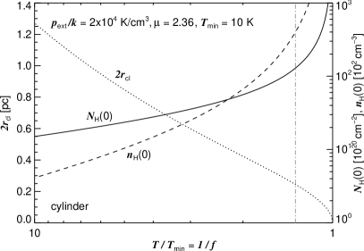
Figure 9: Physical parameters of an isothermal self-gravitating cylinder (left panel) and sphere (right panel) with fixed $p_{\rm ext}/k=2\times 10^{4}\leavevmode\nobreak\ {\rm K\leavevmode\nobreak\ cm}^{-3}$ as a function of cloud temperature. Plotted are the cloud diameter ($2r_{\rm cl}$, dotted line, scale on left axis), the central density (dashed line, right axis), and the column density through the cloud centre (solid line, right axis). The values given for the size and the density depend on the minimum temperature $T_{\rm min}$ assumed to be $10\leavevmode\nobreak\ {\rm K}$. For spherical clouds the parameters are shown for all physical solutions including the supercritical ones characterized through an overpressure larger than $p_{\rm c}/p_{\rm ext}\approx 14.04$. The grey dashed-dotted line in the left hand figure gives the temperature ratio for $f_{\rm cyl}=0.75$.

In the previous sections we have examined how the physical properties of isothermal self-gravitating cylinders and spheres, subject to a fixed external pressure and with a fixed $K$ or temperature, change with the mass, parameterized through the mass ratio $f$. We can therefore directly understand how the properties would be affected by a change of mass, say through accretion of additional material.

In this and the following subsection we discuss how the physical parameters are affected by altering the external pressure and the temperature (through cooling), respectively.

3.6.1 Changing external pressure

As we have seen in Sect. 2.2, the maximum mass line density of a cylinder does not depend on the external pressure. Therefore, in the case of constant mass line density $f_{\rm cyl}$ and fixed temperature, a change of the external pressure has no effect on the gravitational state. In a quasi-equilibrium situation a cylinder can always compensate for a higher external pressure through compression; the central pressure rises so that the overpressure (Eq. 8) remains the same. While a change of the external pressure has no effect on the density profile it does affect the appearance because a cylinder becomes more opaque in higher pressure regions in accordance with $N_{\rm H}(0)\propto\sqrt{p_{\rm ext}}$ (Eq. 18).

The case of a sphere with constant temperature and constant mass $M$ is quite different; a change of the external pressure affects the gravitational state. The ratio of $M$ to the critical mass changes as $f_{\rm sph}=\sqrt{p_{\rm ext}/p_{\rm ext}^{\rm crit}}$, where $p_{\rm ext}^{\rm crit}$ is the maximum possible pressure that the cloud of fixed $M$ can sustain at its edge (see Eq. 6). As the external pressure is increased the central pressure reaches a finite maximum $14.04p_{\rm crit}$ when $f_{\rm sph}=1$, after which there is no stable configuration.

Furthering the discussion in Sect. 2.2, a cloud is considered to be stable if the compression leads to a pressure increase at the cloud edge, i.e., the response $-({\rm d}p(r_{\rm cl})/{\rm d}r_{\rm cl})>0$ where $r_{\rm cl}$ is the cloud radius. Subcritical spheres, those with overpressure below 14.04, are stable against compression with a pressure response $-({\rm d}p(r_{\rm sph})/{\rm d}r_{\rm shp})>0$. Just above the critical state, a sphere is unstable. However, we also note that supercritical spheres significantly above the critical overpressure are not all unstable according to the above definition.

In the case of a cylinder the response is simply given by

$$-\frac{{\rm d}p(r_{\rm cyl})}{{\rm d}r_{\rm cyl}}=2\frac{p(r_{\rm cyl})}{r_{\rm cyl}}>0$$ (39)

for all mass ratios $0<f_{\rm cyl}<1$. Because of this, all gravitational states are stable. In the context of the equilibrium solutions being discussed, there is no critical state (or supercritical states) for cylinders as there is for spheres (see also Ebert 1955; McCrea 1957).

3.6.2 Embedded filaments

Filaments are often characterized by comparing their mass line density to the maximum value $2K/G$. A basic problem of interpretation which arises concerns the effective temperature of the filament, in particular if the filament itself is not entirely isothermal. For example, larger filaments with a relatively high effective temperature of 50 K or more might form/contain small dense interior filaments which are a factor five or more colder. The profile of the column density would show a narrow distribution on top of a broader one. The small size of the narrow feature is related to the colder gas temperature and to its higher external pressure, which in this case is the pressure in the interior in the broad filament. Depending on the distribution of mass assigned, both broad and narrow filaments might be below their relevant maximum mass line density (the fact that they were observed would suggest this conclusion). See further discussion in Sects. 4.2 and 5.3.

3.7 Dependence on temperature

To understand how the isothermal self-gravitating clouds are affected though cloud cooling we consider a spherical cloud of fixed mass and a cylindrical filament with fixed mass line density. For a given external pressure, equilibrium solutions of isothermal self-gravitating clouds exist only above a temperature $T_{\rm min}$. For a sphere, $T_{\rm min}$ is the temperature corresponding to the critical stable cloud, from Eq. 6 for the fixed mass. For a cylinder, $T_{\rm min}$ derives from Eq. 5 for the fixed mass line density. Mathematically we can express ratio of the temperature to $T_{\rm min}$ in terms of $f$ and so the gravitational state of the cloud is given by $T/T_{\rm min}\geq 1$. For spheres $T/T_{\rm min}=1/\sqrt{f_{\rm sph}}$ and for cylinders $T/T_{\rm min}=1/f_{\rm cyl}$.

The cloud parameters (diameter, central density, and column density) for both cylinders and spheres are shown in Fig. 9 where as a minimum temperature we have chosen $T_{\rm min}=10\leavevmode\nobreak\ {\rm K}$. As the cloud cools at fixed mass line density and $p_{\rm ext}$, its size shrinks while both central density and the column density through the centre rise. The variation of the radius and central density with temperature is stronger in the case of a cylinder compared to a sphere. For a given temperature ratio, the central column density through a cylinder is larger than that through a sphere if we neglect the complication of supercritical stable cases.

As it cooled to $T_{\rm min}$, a cylinder would approach asymptotically a singular state of an infinitely thin cylinder with infinite overpressure, assuming it was not in the meantime fragmented through instabilities. At a lower temperature still, there would not be an equilibrium solution at all: it would collapse to a spindle.

Through cooling a sphere reaches the critical point beyond which further cooling would cause a pressure drop at the cloud edge so that the cloud would collapse in a free fall time. The physical solutions presented in Fig. 9 for pressurized supercritical spheres correspond to cloud temperatures above the critical temperature; these supercritical spheres are not accessible simply by cooling at fixed mass and external pressure.

For fixed low mass or low mass line density $T_{\rm min}$ might lie at a value that cannot be reached by any efficient cooling mechanism. For example Bok globules show temperatures not much lower than typical 10 K (Myers et al. 1983; Benson & Myers 1989). See also Appendix A.4. Clouds with $T_{\rm min}$ below this empirical physical limit would therefore remain as gravitational stable equilibrium configurations. A filament might possibly enhance its mass line density through accretion, raising $T_{\rm min}$ and obviating this cooling barrier. Such spheres would also need to accrete more material to become physically unstable and/or they might become unstable through increased compression which raises $T_{\rm min}$ as $p_{\rm ext}^{1/4}$.

4 Observed physical parameters of filaments

In the following we validate the model by comparing the theoretical prediction with recent observations. This is important to confirm because then application of this model to interstellar filaments would allow an independent estimate of astrophysical quantities. For example, it could be used to estimate the interstellar pressure and the distance to cloud complexes and star formation regions, and it could be used in combination of measurements of the dust emission to estimate the dust emissivity.

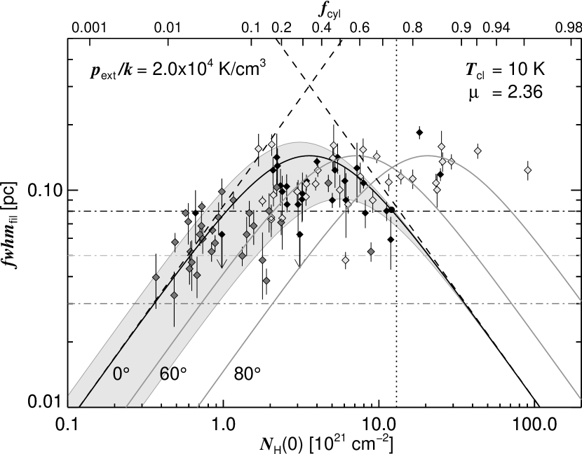
Figure 10: fwhm-$N_{\rm H}(0)$ relation of filaments. Observed values in Polaris (dark grey symbols), IC 5146 (black symbols), and Aquila (light grey symbols), from Fig. 7 of Arzoumanian et al. (2011). Note that we are plotting the column density of H nucleons rather than H₂. We also lowered their values by 2.33/2.8 to correct for the value of $\bar{\mu}$ that they adopted. The horizontal dashed-dotted lines give the imaging resolution achieved in the three fields (black: IC 5146, dark grey: Polaris, light grey: Aquila). Predictions from the model of pressure-confined isothermal self-gravitating cylinders are given for three different inclination angles ($0^{\circ}$, $60^{\circ}$, and $80^{\circ}$; solid black and grey curves). The cloud temperature of the molecular gas is taken to be $T=10\leavevmode\nobreak\ {\rm K}$. The external pressure provided by the ambient medium is assumed to be $p_{\rm ext}/k=2\times 10^{4}\leavevmode\nobreak\ {\rm K\leavevmode\nobreak\ cm}^{-3}$ (see discussion in Appendix A.3). The dashed lines are the asymptotes for low and high overpressure $p_{\rm c}/p_{\rm ext}$ or $f_{\rm cyl}$ (this is a logarithmic version of Fig. 8). For an overpressure corresponding to that of a critical stable sphere, and for inclination $0^{\circ}$, the expected value is shown as the filled black circle. Likewise, the vertical dotted line indicates the column density of a cylinder with mass ratio $f_{\rm cyl}=0.75$; the upper non-linear scale indicates other values of $f_{\rm cyl}$ for this inclination. The expected range for a pressure regime 1.5 to $5\times 10^{4}\leavevmode\nobreak\ {\rm K\leavevmode\nobreak\ cm}^{-3}$ is shown by light grey shading.

Imaging submillimetre observations with Herschel provide estimates of the fwhm of the filaments, their density profiles, and of the central column densities. Some uncertainties relating to such measurements are discussed in Appendix A. Here, we discuss the results for individual filaments in Polaris, IC 5146, and Aquila presented by Arzoumanian et al. (2011). To describe the filament profiles, they adopted a generalization of Eq. 2 for the density profile, parameterized by index $\alpha$:

$$\rho(r)=\rho_{\rm c}(1+(r/\sqrt{8}r_{0})^{2})^{-\alpha/2}.$$ (40)

At large cloud radii ($r\gg\sqrt{8}r_{0}$) the profiles of the filaments in IC 5146 indicated $\alpha\sim 1.6\pm 0.3$, less steep than the value four they expected for clouds in a vacuum, in agreement with previous measurements discussed by Fiege & Pudritz (2000). Our interpretation is simply that an equilibrium cylinder that is pressure confined is the relevant model. Relatively flat profiles are a natural outcome for cylinders with a mass ratio $f_{\rm cyl}$ considerably smaller than unity (Section 3.3).

In Fig. 10 the deconvolved fwhm and $N_{\rm H}(0)$ results of Arzoumanian et al. (2011) are compared with the self-consistent prediction of our model of pressure-confined cylinders, including the asymptotic behaviours. The parameters for the filaments of the three observed regions occupy different areas in the fwhm-$N_{\rm H}(0)$ plane. The filaments in Polaris show the lowest central column densities with most values below $N_{\rm H}(0)<10^{21}\leavevmode\nobreak\ {\rm cm^{-2}}$. The sizes are also apparently smaller compared to the two other samples. The filaments in IC 5146 have intermediate central column densities with a mean $N_{\rm H}\sim 6\times 10^{21}\leavevmode\nobreak\ {\rm cm^{2}}$. The highest column densities were observed for filamentary structures in Aquila with values up to $\sim 10^{23}\leavevmode\nobreak\ {\rm cm^{-2}}$. Overall, the data indicate a trend that filaments with low column densities are on average smaller than those with high column densities.

As we see in Fig. 10 the model of pressurized cylinders shows a good agreement with the observations, although obvious deviations do exist. The observations are broadly consistent with a cloud temperature $T=10\leavevmode\nobreak\ {\rm K}$ and an ambient pressure of $p_{\rm ext}/k=2\times 10^{4}\leavevmode\nobreak\ {\rm K\leavevmode\nobreak\ cm}^{-3}$. Such a pressure is in the range expected, as discussed in Appendix A.3. The data show a dispersion around the theoretical curve which can be attributed to a variation of the external pressure alone. Most data points lie in a pressure regime $p_{\rm ext}/k$ from $1.5\times 10^{4}\leavevmode\nobreak\ {\rm K\leavevmode\nobreak\ cm}^{-3}$ to $5\times 10^{4}\leavevmode\nobreak\ {\rm K\leavevmode\nobreak\ cm}^{-3}$. Note how the position of the maximum lies on a line parallel to the high $f_{\rm cyl}$ asymptote. An additional horizontal deviation of data from the model is expected because of the distribution of inclination angles; as shown in Fig. 10, higher inclination could in principle explain some of the high values of the column densities. Note that at constant pressure, the fwhm-$N_{\rm H}(0)$ curve translates vertically with $T$.

Kandori et al. (2005) studied the physical parameters of Bok Globules using an idealized model of a pressurized isothermal self-gravitating sphere to fit the column density profile obtained from extinction measurements. The derived external pressures ranged from $2.1\times 10^{4}\leavevmode\nobreak\ {\rm K\leavevmode\nobreak\ cm}^{-3}$ to $1.8\times 10^{5}\leavevmode\nobreak\ {\rm K\leavevmode\nobreak\ cm}^{-3}$ with a mean of $5.7\times 10^{4}\leavevmode\nobreak\ {\rm K\leavevmode\nobreak\ cm}^{-3}$. There is overlap with the pressures derived here but on average they are higher.

4.1 Behaviour at small column density

Comparison of the data to the asymptotic behaviour at low $f_{\rm cyl}$ (Eq. 62) constrains the ratio $T/p_{\rm ext}$. In combination with this, the position of the maximum (Eq. 32) constrains $T$. At low column density, a higher pressure could be accommodated by raising $T$, but for higher column densities near the predicted maximum the fwhm might become too large. Likewise, if no efficient cooling mechanisms exist to cool the cloud temperature below $10\leavevmode\nobreak\ {\rm K}$, then we have a lower limit on the required external pressure close to the cited values.

The parameters of most of the filaments in Polaris seem to follow the relation expected for rather low mass ratio, $f_{\rm cyl}<0.1$. Those structures are therefore not strongly self-gravitating and so possibly transient density enhancements. If they exist, filaments with even lower $f_{\rm cyl}$ would be small compared to the instrumental resolution and of low contrast in the images. Stronger background fluctuations (cirrus noise; e.g., Martin et al. 2010) in the other two cloud complexes would produce a more challenging limitation to identifying faint low column density structures, and so the fact that filaments with low mass ratio are less frequent or entirely absent in the two other samples might result from this selection effect.

4.2 Behaviour at large column density

We think that inclination effects are unlikely responsible for the extremely high column densities reported. High column densities without the expected small sizes might instead be related to cold filaments which are embedded and pressure-confined within larger filamentary structures, as mentioned in Sect. 3.6.2. Our simple idealized model is therefore not easily applicable.

For example, in the IC 5146 sample, the filament with the highest column density (numbered 6 by Arzoumanian et al. 2011) also has the highest reported mass line density (152 M_⊙ pc^-1), much higher than the expected maximum value for a filament with $K$ corresponding to 10 K. This is a very interesting but complex filament with large variations in central column density and fwhm along the sinuous ridge. The images and average line profile show one or more cold irregular inner filaments inside a broader structure. The narrow filaments are often paired in parallel segments. How high the mass line density is judged to be depends on how far out radially the column density is integrated and this depends on where the adopted model profile meets the “background.” Measurement of the embedded filament(s) above the complex background of the broad filament would produce physical parameters closer to the simple model. A slightly higher $K$ would help too, moving the predicted curve vertically in Fig. 10.

Our sense is that this whole filament is not in free fall radial collapse, in which case the self-gravity of the larger embedding structure needs to be balanced too; an isothermal model is probably not appropriate, but a higher $K$ (or perhaps even extra magnetic pressure) would be needed. This is open to experimental investigation by molecular velocity and line-width measurements such as reported by Pineda et al. (2010). Kramer et al. (1999) have in fact mapped a 0.4 pc square region on the ridge of this filament in some lines of the rare isotopologues of CO. Even within this small region they find many clumps and two ridges with differing velocites and line widths. Overall this dense central region, while clumpy, is fairly cold in terms of $K$ though perhaps warmer than 10 K. On the other hand, for ¹³CO on a larger scale (2.5 pc) the velocity dispersion $\sigma\approx 1$ km s^-1 (position C3 in Dobashi et al. 1992). While perhaps exaggerated by optical depth effects, this is suggestive of $K$ being an order of magnitude larger in the broad embedding filament. The situation seems to be similar for the widest filament (numbered 12) where the profile suggests an interior cold (sometimes paired) filamentary structure surrounded by a more turbulent gas.

Interestingly, no filaments with high central extinction ($N_{\rm H}(0)>\sim 2\times 10^{22}\leavevmode\nobreak\ {\rm cm^{-2}}$) and the corresponding low size (${\it{fwhm}}<0.08\leavevmode\nobreak\ {\rm pc}$) were found. There is no obvious selection effect against finding these high $f_{\rm cyl}$ filaments though, as suggested above, measurement of their parameters might be an issue depending on their environment.

If strongly self-gravitating filaments, those above a certain mass ratio, do not exist, then why? This might be inherent to the process responsible for the formation and evolution of filaments generally, or might be because of their disruption and/or short lifetimes. While interesting, the former possibility is beyond the scope of this paper. One clue to the latter possibility is that according Fig. 10 the empirical cut-off in $f_{\rm cyl}$ is near 0.75, where the cylinders have about the same overpressure as a critical stable sphere and so if appropriately fragmented might form structures that would collapse. This is explored further in the following section.

5 Structure formation along filaments

In most cases observed filaments show substructure, contributing to the difficulty of measuring their parameters. Most interesting for understanding the potential role of filaments, as opposed to just high column and volume density, in the star formation process are the condensed structures extracted, “prestellar cores” having strong self-gravity. By definition they are cool, not having detectable emission at 70 $\mu$m or 24 $\mu$m (Könyves et al. 2010), and so while they have the potential for forming protostars or young stellar objects (YSOs) (André et al. 2010) they are not yet vigorously doing so. They are being externally heated (stage E, Roy et al. 2011) with little internal energy being generated. These “prestellar cores” appear in the higher column density filaments at typically $A_{V}>8\leavevmode\nobreak\ {\rm mag}$, as in Aquila and IC 5146 (André et al. 2010; Arzoumanian et al. 2011). Cold protostars are rarer and also often associated with filaments (André et al. 2010; Bontemps et al. 2010).

Even filaments with much lower column density, those with low $f_{\rm cyl}$ such as in Polaris, have substructure. These are dubbed “starless cores” as well, potentially confusing nomenclature: although they have sizes typical of what defines cores (radii less than a few tenths of a parsec) they comprise much less than a solar mass and are not significantly gravitationally bound and so do not seem destined to form stars (André et al. 2010) .

5.1 Equilibrium filaments

If the basic structure is described by an equilibrium filament, as we have argued, then the question arises as to the origin of the substructure. Equilibrium filaments are subject to gravitational instabilities that are axisymmetric, producing structure along the axial directions. Two types may be distinguished (Nagasawa 1987). For high $f_{\rm cyl}$ ($r_{\rm cyl}\gg\sqrt{8}r_{0}$) the instability forms out of compression. A local density increase raises the self-gravity and lowers the gravitational energy, leading to a growth in the amplitude of the structure. For low $f_{\rm cyl}$, those with a fairly flat profile ($r_{\rm cyl}\ll\sqrt{8}r_{0}$), the instability relates to deformation of the surface; in such a “sausage instability” it is the volume energy of the surface integral of the external pressure that is lowered. Transitional behaviour mixing these cases occurs near $f_{\rm cyl}=1/2$ ($r_{\rm cyl}=\sqrt{8}r_{0}$).

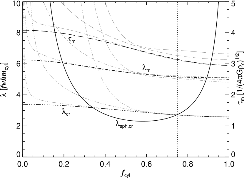
Figure 11: Length and time scales relevant to fragmentation as a function of $f_{\rm cyl}$, in units of the fwhm (left axis) and $1/\sqrt{4\pi G\rho_{c}}$, the sound crossing time of $r_{0}$ (right), respectively. The shortest wavelength growing mode is $\lambda_{\rm cr}$ (dashed-multiple dotted lines). The fastest growing mode is $\lambda_{\rm m}$ (dashed-single dotted lines) which, in the linear regime, develops on a time scale $\tau_{\rm m}$ (long-dashed lines). For comparison, $\lambda_{\rm cr,sph}$ is the length along the filament required to encompass a mass equal to that of a critical stable sphere for the same $p_{\rm ext}$ and $K$ (solid line). The black broken lines correspond to non-magnetized cylinders. The related grey lines show the increasing effect of a magnetic field and correspond to $p^{2}=1\%$, $10\%$, and $100\%$ of equipartition. The values are based on the work of Nagasawa (1987), see App. E. The vertical dotted line marks the mass ratio $f_{\rm cyl}=0.75$.

Linear analysis of the dispersion relation (Nagasawa 1987) shows that the critical wavelength above which perturbations grow is, for $f_{\rm cyl}\rightarrow 1$,

$$\lambda_{\rm cr}=3.96\,\sqrt{8}r_{0}=3.96\,r_{\rm cyl}\sqrt{(1-f_{\rm cyl})}=2.58\,{\it{fwhm}}_{\rm cyl}$$ (41)

and, for $f_{\rm cyl}\rightarrow 0$,

$$\lambda_{\rm cr}=5.87\,r_{\rm cyl}=5.87\,\sqrt{f_{\rm cyl}}\sqrt{8}r_{0}=3.39\,{\it{fwhm}}_{\rm cyl},$$ (42)

with a smooth variation for values of $f_{\rm cyl}$ in between. The wavelength corresponding to the maximum growth rate, $\lambda_{\rm m}$, is about twice $\lambda_{\rm cr}$ (a factor 1.96 and 1.84 for the above limiting cases, respectively). Figure 11 shows the $f_{\rm cyl}$ dependence of $\lambda_{\rm cr}$ and $\lambda_{\rm m}$, relative to the fwhm. At least initially, the fastest growing mode is quite elongated, with $\lambda_{\rm m}/{\it{fwhm}}_{\rm cyl}\approx 5$. This would also be the separation of the cores, in units of fwhm. But in absolute terms, both $\lambda_{\rm m}$ and fwhm become arbitrarily small in the two limits. This is shown in Figure 12.

Figure 12: Like Fig. 11, but with lengths and time scales expressed in physical units. The molecular cylinders are assumed to have temperatures of $T_{\rm cl}=10\leavevmode\nobreak\ {\rm K}$ and to be pressurized by a medium with $p_{\rm ext}/k=2\times 10^{4}\leavevmode\nobreak\ {\rm K/cm^{3}}$. Also shown is the corresponding fwhm (see Fig. 7).

An important issue is the growth time scale, which is proportional to $1/\sqrt{4\pi G\rho_{\rm c}}=r_{0}/\sqrt{K}$, the sound crossing time across $r_{0}$. As shown in Fig. 11, for the fastest growing mode the constant of proportionality falls from 4.08 to 2.95 as $f_{\rm cyl}$ increases from 0 to 1 (Nagasawa 1987). It is also convenient to define a time scale $\tau_{\rm Kp}=\sqrt{K/(4\pi Gp_{\rm ext})}$, that evaluates to 0.4 My for the adopted values of $K$ and $p_{\rm ext}$. Thus for $f_{\rm cyl}\rightarrow 1$,

$$\tau_{\rm m}=2.95(1-f_{\rm cyl})\tau_{\rm Kp}.$$ (43)

This clearly arbitrarily short. For $f_{\rm cyl}$ near 0 the time scale is

$$\tau_{\rm m}=4.08\tau_{\rm Kp}.$$ (44)

While this is much faster than the crossing time $r_{\rm cyl}/\sqrt{K}$, because $r_{\rm cyl}\ll r_{0}$, it is still finite, of order 1.6 My for the canonical values, even longer for a warmer or more turbulent gas. This would set up “sausage instabilities.” The time scale $\tau_{\rm m}$ in My is shown in Figure 12.

The effect of a uniform magnetic field along the filament has also been studied by Nagasawa (1987). The “compressive instability” (finite $f_{\rm cyl}$) is not much affected because the field is axial, but the “sausage instability” (low $f_{\rm cyl}$) is strongly suppressed because the field limits the surface distortion. In that case, both $\lambda_{\rm m}$ (see Fig. 11) and the time scale $\tau_{\rm m}$ are increased significantly, even for a field much smaller than equipartition strength (where $p^{2}=B^{2}/(4\pi\rho_{c}K)=1$). Thus, in the ISM this instability seems unlikely to be relevant to determining the substructure seen in filaments with low mass fraction as in Polaris.

The question of the final outcome of the non-linear growth of the “compressive instability” is of course critical. Curry (2000) found a sequence of equilibrium structures within filaments. Their shape is prolate along the cylinder axis, within a tidal lobe within which the equidensity contours are closed. These equilibria are gravitationally dominated and so are rounder as the pressure (density) contrast between centre and lobe increases (limiting axial ratio about 1.7). The behaviour of the lobe radius and the mass contained within the lobe with increasing pressure contrast is reminiscent of the Bonnor-Ebert sequence, though it is not known whether these cores become unstable to collapse at similar overpressures.

The non-linear growth of the instability has been followed numerically by Inutsuka & Miyama (1997) for two cases of equilibrium cylinders with $f_{\rm cyl}=0.9$ and 0.2. For the former they find a complete disintegration of the filament into well separated spherical clouds suggestive of gravitational collapse. For the latter a distinctive spherical core forms as well, with the central density increased by a factor nine, but it does not collapse.

5.1.1 Mass of the fragment

The maximum mass available to be concentrated by a perturbation of wavelength $\lambda$ is

$$M_{frag}=\lambda M/l=2\sqrt{8}f_{\rm cyl}(1-f_{\rm cyl})\frac{\lambda}{\sqrt{8}r_{0}}\frac{K^{2}}{\sqrt{4\pi G^{3}p_{\rm ext}}}.$$ (45)

This is deliberately cast in the same form as Eq. 6 for the mass of a critical stable sphere, where the prefactor is simply 4.191.

Even if the growth of the perturbation is effective in concentrating material into a fairly spherical core, it seems intuitive to us that the outcome is unlikely to be gravitational collapse unless the mass of the core is comparable to the critical Bonnor-Ebert mass for the external pressure confining the original cylinder. To accumulate the critical mass, the required wavelength $\lambda_{\rm sph,cr}$ is, when $f_{\rm cyl}$ is close to 1,

$$\lambda_{\rm sph,cr}/{\it{fwhm}}_{\rm cyl}=4.191/\left(4\sqrt{8}\sqrt{2^{2/3}-1}f_{\rm cyl}(1-f_{\rm cyl})\right)$$ (46)

and, when $f_{\rm cyl}$ is close to 0,

$$\lambda_{\rm sph,cr}/{\it{fwhm}}_{\rm cyl}=4.191/\left(2\sqrt{3}\sqrt{8}f_{\rm cyl}\sqrt{f_{\rm cyl}(1-f_{\rm cyl})}\right).$$ (47)

Thus for both of these limiting cases the perturbations would initially have to be extremely elongated compared to the fwhm. The locus of $\lambda_{\rm sph,cr}/{\it{fwhm}}_{\rm cyl}$ in Figure 11 contrasts these extreme values with the finite value of $\lambda_{\rm m}/{\it{fwhm}}_{\rm cyl}$ (in the range 5 – 6). Thus in both limits of $f_{\rm cyl}$, any condensations resulting from perturbations would be of low mass compared to the critical Bonnor-Ebert mass; this is not a promising scenario for forming prestellar or protostellar cores.

Indeed none are observed for filaments with low $f_{\rm cyl}$. Also, because of suppression by the magnetic field, we are less interested in the case $f_{\rm cyl}$ close to 0. It is hard to imagine a perfectly uniform filament being created in a turbulent medium; whether the structure that does exist is just a natural by-product of formation of the filament needs to be investigated.

For filaments with very high overpressure, or $f_{\rm cyl}$ close to unity, the implication is that a series of small dense condensations would develop, each of insufficient mass to collapse. On a longer time scale these might merge to form more massive cores (Inutsuka & Miyama 1997), perhaps arriving at the high density equilibrium configuration found by Curry (2000). According to the findings presented in Fig. 10 this $f_{\rm cyl}\rightarrow 1$ limiting case has little relevance to the interstellar medium as the precursor narrow high column density filaments have not been observed. How far the results are biased through the method applied to characterize highly opaque filaments need to investigate as well.

However, for intermediate $f_{\rm cyl}$ we see in Figure 11 that $\lambda_{\rm sph,cr}$ can actually be less than $\lambda_{\rm m}$ (and even $\lambda_{\rm cr}$) and comparable to the fwhm. This is a more propitious situation, starting from a much less elongated perturbation, to accumulate a mass comparable to the critical Bonnor-Ebert mass.

For such intermediate $f_{\rm cyl}$, $\tau_{\rm m}\approx 3.5(1-f_{\rm cyl})\tau_{\rm Kp}$. This is sufficiently rapid (Fig. 12) that initially uniform filaments could develop structure on astronomically relevant timescales. As discussed above, it seems plausible that some of these could accumulate a critical Bonnor-Ebert mass and become the observed cold protostars. If this were the explanation, then the protostars ought to be separated by about $\lambda_{\rm m}$, about five times the fwhm of the embedding/undisturbed filament (Fig. 11). This appears to be on the order of what is observed (see below) but needs to be carefully quantified.

5.2 Pearls on a string

According to Men’shchikov et al. (2010), the above-mentioned prestellar cores, observed along high column density filaments, are about the same size as the width of the filament. Inspection of the images of source positions presented (Men’shchikov et al. 2010; Arzoumanian et al. 2011) shows that they are also separated by about the fwhm of the filament. Therefore, remarkably, they are arranged “almost like pearls on threads in a necklace” (Men’shchikov et al. 2010). Because of the small separation it appears unlikely that those structures are caused directly by the gravitational instabilities discussed above. We have seen that condensations resulting from that origin would have a separation of at least 2.5 times the fwhm (for intermediate mass ratios $f_{\rm cyl}>\approx 0.5$). We have examined the above-mentioned filament 6 in IC 5146 in both SCUBA (Di Francesco et al. 2008) and Herschel archival submillimetre images. There are many clumps that would be extracted as prestellar cores, but not all are equal, and our impression is that these are somewhat clustered with major concentrations typically separated by 2’ to 5’, corresponding to 2.2 to 5.5 times the given fwhm. The YSOs associated with this filament found in the Spitzer study by Harvey et al. (2008) are also well separated. This is perhaps more in line with what would be expected from gravitational instabilities, but then a hierarchy and perhaps time sequence of fragmentation is suggested.

At this point, we feel that the origin of the substructure is an open question. Other than gravitational instability, perhaps it is a natural consequence of the formation of such filaments; in the presence of strong self-gravity, it might be difficult to form a perfectly straight and uniform cylinder. In our experience it is also a challenge to extract and characterize “sources” found as closely spaced inhomogeneities along a filament.

Because a separation of one fwhm is less than $\lambda_{\rm cr,sph}$ (Fig. 11), these prestellar cores, while strongly self-gravitating, would probably be stable against collapse, consistent with their being starless. Whether these presently starless clouds will form any stars in the future and therefore be relevant to the initial mass function of the stars is also an interesting open question.

5.3 Filaments with high mass line density

For a filamentary structure with more than the maximum mass line density (Eq. 4), there is no equilibrium solution. If they could be created, somehow, because of their high density they would collapse on a rapid timescale.

There are certainly filamentary configurations observed that have a large mass line density, considerably greater than the maximum line density if evaluated for $K$ corresponding to a low value like 10 K which we find appropriate to simple narrow filaments. André et al. (2010) conclude that the gravitational fragmentation of such “supercritical” filaments is responsible for the formation of the observed self-gravitating prestellar cores and protostars. There are two problems with this scenario.

First, our interpretation of the numerical calculations of Inutsuka & Miyama (1997) is that there is fragmentation only if the mass line density is finely tuned to being just above the maximum value and/or if the initial conditions already contain large perturbations, which begs the question. Perhaps a relevant configuration could be set up beginning with an equilibrium filament with $f_{\rm cyl}$ close to 1 and then making it “supercritical” by lowering the temperature. Otherwise, the predominant outcome is radial collapse of the cylinder to a spindle. Eventually the collapsing spindle would become optically thick and could develop substructure; but this would be on a small scale because of the large density and small size of the collapsed filament (Inutsuka & Miyama 1997).

Second, in the process of forming the fragments, a “supercritical” filament itself would collapse, be consumed, and disappear on the same rapid time scale. However, the observations indicate that prestellar cores, and even YSOs, occur along identifiable filaments of finite size, even if it appears that the mass line density is “supercritical.” This coexistence is a challenge to be satisfied by any model of the structure formation, even for initially equilibrium filaments.

While high column and volume density are arguably fundamental to any process of fragmentation, our conclusion is that protostar and cluster formation must be a more complex process than simply the gravitational fragmentation of “supercritical” filaments. Based on the complex radial profiles of these high mass line density filaments, we think that some progress might be made by considering cold embedded filaments within a broader structure supported by a gas with higher effective $K$, in which case the overall configuration is not actually “supercritical” and in free fall.

6 Summary and discussion

We have analyzed the physical properties of interstellar filaments on the basis of an idealized model of isothermal self-gravitating infinitely long cylinders which are pressurized by the ambient medium. The pressure-confined cylinders have a mass-line density smaller than cylinders extending into a vacuum. The mass fraction $f_{\rm cyl}$, the ratio of the mass-line density to the maximum possible for equilibrium configurations, describes the gravitational state of the cylinder. For given temperature and external pressure, it is used in deriving analytical expressions for the central density, the radius, the column density profile, the central and average column densities and the fwhm. The dependence of the physical properties on external pressure and temperature is clear in these expressions. The results are compared to the case of pressure-confined isothermal self-gravitating (Bonnor-Ebert) spheres, characterized by the mass fraction $f_{\rm sph}$, the ratio of the mass to the mass of the critical stable sphere.

We compared the model prediction for the relation between the size and the central column density with recent observations of filaments. Given the complexity seen it is gratifying to find good agreement, even surprising considering the idealization of the model. In practice the model seems best applicable to those filaments that are cold and show a simple smooth elongated structure. On the basis of the model the filaments appear to experience an ambient pressure $p_{\rm ext}/k$ in the range $1.5\times 10^{4}\leavevmode\nobreak\ {\rm K\leavevmode\nobreak\ cm^{-3}}$ to $5\times 10^{4}\leavevmode\nobreak\ {\rm K\leavevmode\nobreak\ cm}^{-3}$ and to have a gas temperature $T\approx 10\leavevmode\nobreak\ {\rm K}$. For these parameters, the observations indicate an apparent physical upper limit to the mass ratio $f_{\rm cyl}\approx 0.75$; higher column density narrower filaments are not seen. The corresponding maximum central extinction for the observed filaments fitting the model is $A_{V}\approx 7\leavevmode\nobreak\ {\rm mag}$. This is interestingly close to the empirical threshold for star formation, but we think this is coincidental, especially given the variable threshold from region to region (Enoch et al. 2007).

We have summarized and discussed previous stability studies that have shown that all unmagnetized infinitely long cylinders $f_{\rm cyl}<1$ are subject to gravitational instabilities. While a magnetic field can have a stabilizing effect for $f_{\rm cyl}<0.5$, in particular suppressing “sausage instabilities” for $f_{\rm cyl}\approx 0$, there is a negligible effect on compressive instabilities for $f_{\rm cyl}>0.5$. Interstellar magnetized filaments would seem to become increasingly unstable towards large $f_{\rm cyl}$ because of a strongly increasing growth rate of the instabilities. The disintegration of filaments close to the maximum mass line density ($f_{\rm cyl}>0.9$) would produce fragments whose masses are well below the critical value to form stars. We found no indication in the theory for a strong threshold for the formation of fragments that would collapse. However, intermediate values of $f_{\rm cyl}$ seem most favorable. The fastest growing disturbance for $f_{\rm cyl}>0.5$ occurs at a length approximately five times the fwhm, so that protostars or clusters would be well separated.

It is difficult to understand in this model why in high column density filaments there would be substructure akin to the extracted prestellar cores separated along the filament by only one fwhm, which is well below the minimum length at which a disturbance would grow ($\lambda_{\rm crit}>\approx 2.5\times{\it{fwhm}}_{\rm cyl}$). This might point to external influences accompanying the process that formed the filament in the first place, resulting in the non-uniform mass line density along these filaments, not the idealized model considered here. On the other hand, if one concentrates on the major mass concentrations along the filament, their separation might be more compatible with an origin in gravitational instability along the cylinder.

High mass line density filaments are observed that would appear to have more than the maximum mass line density that could exist in equilibrium, at least if evaluated for the low adopted $K$. The coexistence of embedded narrow high column density filaments, even in pairs, and considerable substructure (prestellar cores) and protostars suggests to us a scenario more complex than simply the free-fall collapse and fragmentation of cylinders with more than the maximum line density. Although the simple model cannot explain such complex structure, it points to a situation in which the embedding structure is supported by gas with a $K$ larger than the low value that might reasonably be adopted for the narrow embedded structure. This is obviously open to observational scrutiny via mapping of velocities and line widths of appropriate molecules.

As McCrea (1957) has emphasized, “genuine” gravitational collapse to form stars and clusters is best realized in configurations with roughly the same dimensions in all directions so that gravitational effects are three-dimensional. He argued that the breakup of less favorable one-dimensional configurations like filaments must be due to irregularities in the density distribution and the external pressure to which they are subjected, or to differential motions. Empirically, there is suggestive evidence that such breaking of the symmetry of an idealized long cylinder is important, as occurs for example where filaments appear to cross. These are matters that could be explored now in the results of numerical simulations.

Appendix A Questions of scale

In comparing the models with the data we need to be aware of the context, what can be measured and the related uncertainties. In this appendix we discuss column density, size, external pressure, and effective temperature.

A.1 Column density

Column densities of filaments from Herschel data are fundamentally in units of the dust optical depth in the submillimetre. This is converted to $N_{\rm H}$ using a submillimetre dust opacity. This opacity appears to show a dependence on environment and might be uncertain by a factor two (Martin et al. 2011). For the overview comparison in Figure 10, where $N_{\rm H}(0)$ is on a logarithmic scale, this is might not be a major concern.

In the diffuse and largely atomic interstellar medium, where both $N_{\rm H}$ and optical interstellar extinction curves can be observed directly, we have the ratio $N_{\rm H}/E(B-V)=5.8\times 10^{21}{\rm cm^{-2}/mag}$ (Bohlin et al. 1978) and an absolute to relative extinction $R_{V}=A_{V}/E(B-V)=3.1$ (Fitzpatrick 1999). A column density of $10^{22}\leavevmode\nobreak\ {\rm cm^{-2}}$ therefore corresponds to $A_{V}=5.3$ mag. We use this same conversion when $A_{V}$ is being used a “shorthand” for column density in dense molecular environments, recognizing that the actual visual extinction, if it could be measured, would probably not be this value.

Another measure more applicable at higher column densities is near infrared colour excess. This is also often converted to $A_{V}$, which again should be regarded as a “shorthand” because the shape of the interstellar extinction curve through the optical probably varies. It might be more reliable to convert the near infrared colour excess directly to $N_{\rm H}$, but that calibration is not actually known for the high column densities encountered in star-forming regions (Martin et al. 2011).

Another uncertainty might be related to radiative transfer which produces a radial variation of the dust temperature within externally-heated filaments. While the dust opacity seems to be larger for dust in denser environments, the averaging of the dust emission over a distribution of temperatures leads to a reduced effective emission coefficient and a spectral dependence of the emissivity that is less steep than is intrinsic for dust in a diffuse environment as theoretically demonstrated for condensed cores (Fischera 2011). The radiative transfer effects increase with central column density and could therefore play a larger role at high mass ratios. The column density profile indicated by the surface brightness would be flatter than the intrinsic profile.

A.2 Size

Sizes of filaments are measured from the profile of the column density in the direction orthogonal to the axis of the filament. The fwhm could be measured directly but is more usually found as a parameter of a model fit to the profile. The model fit also needs to account for the background on which the filament appears superimposed. In practice both the background and the profile can vary along the filament, adding to the challenges (Arzoumanian et al. 2011 resorted to using a Gaussian model to find the fwhm) and the reported standard deviation in the parameters. Even in nearby molecular clouds, the filaments, while resolved, are often not a lot larger than the imaging resolution. Therefore, the reported sizes have been “deconvolved.” In the future, this might be avoided by forward modeling, adopting analytical models like we have presented, convolving the predictions to the resolution of the data, and then iteratively fitting the parameters.

The background is still something to be fit too. Depending on the circumstances, this background could be from foreground or background material unrelated to the filament, and/or a contribution from the medium providing the pressure confinement. A well-defined edge of a filament might suggest, for example, that the filament can be regarded as cold material which is surrounded by a warmer or more turbulent but less dense environment. This relates to the following discussion of external pressure.

A.3 External pressure

Boulares & Cox (1990) presented a model of the vertical support of the Galactic disk. The mid-plane pressure near the sun is at least $p_{\rm ext}/k=2.5\times 10^{4}$ K cm^-3. About a third of this is the effective vertical support by cosmic rays; however, on the size scale of the structures of interest here, cosmic ray pressure can be ignored Curry & McKee (2000); Fischera & Dopita (2008); Fischera (2011). The remainder is a combination of kinetic pressure (thermal and turbulent motions) and magnetic pressure. For a magnetic field of less than equipartition strength, the kinetic pressure would be at least $0.8\times 10^{4}\leavevmode\nobreak\ {\rm K\leavevmode\nobreak\ cm}^{-3}$. The thermal pressure is only about a third of this (Kalberla & Kerp 2009), the rest being turbulent pressure.

The filaments being discussed are within clouds with sufficient column density to have become molecular ($\left<A_{V}\right>>1$; e.g., Glover & Mac Low 2011). If it is assumed that these clouds can themselves be described as pressure-confined isothermal spheres, with enough self-gravity to be near the critical mass, then following Eq. 21 and Eq. 58 the external pressure required to produce a mass surface density $\left<\Sigma\right>$ averaged over the projected radius is given by

$$p_{\rm ext} = (\pi/8)G\left<\Sigma\right>^{2}\,{\rm or}$$

$$p_{\rm ext}/k = 0.37\times 10^{4}\left<A_{V}\right>^{2}\leavevmode\nobreak\ {\rm K\leavevmode\nobreak\ cm}^{-3}.$$ (48)

A subcritical sphere would require a greater external pressure to produce the same average column density (Fig. 4). The average column density in the GMC sample discussed by Heyer et al. (2009) corresponds to $\left<A_{V}\right>\approx 2.8$, which would require a pressure of $2.9\times 10^{4}\leavevmode\nobreak\ {\rm K\leavevmode\nobreak\ cm}^{-3}$. This seems consistent with the fact that this cloud sample is in the inner Galaxy where the midplane pressure is probably higher.

The central extinction through a critical stable isothermal sphere is $A_{V}=8.0\sqrt{(p_{\rm ext}/k)/(2\times 10^{4}\leavevmode\nobreak\ {\rm K\leavevmode\nobreak\ cm}^{-3}})$ mag (Fischera & Dopita 2008; Fig. 4). This predicted amount of extinction seems to be in agreement with that observed for molecular clouds (Dopita & Sutherland 2003).

Two conclusions are that the midplane pressure is indeed quite high, and that the pressure within the molecular cloud due to its self gravity – the ambient external pressure experienced by the filaments – will be higher still, depending on where the filaments lie within the pressure profile of the molecular cloud.

Another contribution could be due to ram pressure, for example related to the sweeping up of the North Celestial Loop of which the Polaris field is a part.

A.4 Effective temperature

For the model we need the effective temperature embodied in $K$, related to both the thermal and the turbulent (non-thermal) motion of the gas. The most direct way to measure this would be through the line width of an appropriate molecular tracer. For example, the ammonia mapping of B5 in Perseus by Pineda et al. (2010) revealed a sharp decrease in line width in the central 0.1 pc. This is thought to be the result of the decay of supersonic turbulence present on larger scales; the observed line widths are subsonic for a thermal/kinetic temperature of 10 K. Foster et al. (2009) present results from an ammonia survey of many other cores in Perseus and find them mostly quiescent ($\sigma_{\rm nonthermal}\approx 0.12$ km s^-1, but see their histograms for details of the full survey). The modeling of two lines gives kinetic temperatures about 12 K; derived excitation temperatures are lower (Foster et al. 2009). The dust temperature from the submillimetre spectral energy distribution observable by Herschel is typically low (down to 10 K) in the high column density regions in low mass star forming regions (see the temperature maps in, e.g., Bontemps et al. 2010 and Arzoumanian et al. 2011). Coupling of the kinetic temperature in the gas to the dust temperature comes into play for $n_{\rm H2}>10^{4}\leavevmode\nobreak\ {\rm cm}^{-3}$ (Goldsmith 2001). According to Fig. 1, this becomes relevant for strongly self-gravitating cylinders ($f_{\rm cyl}>0.7$). Taken together, while perhaps a platonic ideal, a small dense isothermal core with $K$ corresponding to 10 K is reasonable as a reference value. However, $K$ might be higher than this in some environments or stages of evolution. And of course the structure might not be exactly isothermal.

Appendix B Mean column density of spheres

In paper II the approximation for the mean column densities of cylinders and spheres as a function of the overpressure were presented. Here, we want to comment on the values for spheres and give an exact expression for the asymptotic behaviour at large overpressures.

The mass of a spherical isothermal self-gravitating cloud which is in pressure equilibrium with the surrounding medium ($p(z_{\rm cl})=p_{\rm ext}$) is given by (paper I)

$$M_{\rm sph}=\frac{K^{2}}{\sqrt{4\pi G^{3}p_{\rm ext}}}e^{-w(z)/2}\int_{0}^{z}{\rm d}z^{\prime}\,z^{\prime 2}\,e^{-w(z^{\prime})}.$$ (49)

Here, $w=\phi/K=\ln{p_{c}/p_{\rm ext}}$ is the unit free potential and $z=rA$ the unit free radius of the Lane-Emden equation

$$\frac{1}{z^{2}}\frac{{\rm d}}{{\rm d}z}\left(z^{2}\frac{{\rm d}\omega}{{\rm d}z}\right)=e^{-\omega},$$ (50)

where $A^{2}=1/r_{0}^{2}=4\pi G\rho_{\rm c}/K$. Using the expression for the mass (Eq. 49) and

$$r_{\rm cl}=z_{\rm cl}/A=z_{\rm cl}\frac{K}{\sqrt{4\pi Gp_{\rm ext}}}e^{-\omega(z_{\rm cl})/2},$$ (51)

for the cloud radius we obtain for the mean mass surface density of an isothermal self-gravitating sphere

$$\left<\Sigma\right>(z_{\rm cl})=\frac{M_{\rm sph}(z_{\rm cl})}{\pi r_{\rm sph}^{2}(z_{\rm cl})}=\frac{\sqrt{4\pi Gp_{\rm ext}}}{\pi G}\zeta(z_{\rm cl}),$$ (52)

where

$$\zeta(z_{\rm cl})=\frac{e^{-\omega(z_{\rm cl})/2}\int_{0}^{z_{\rm cl}}{\rm d}z\,z^{2}\,e^{-\omega(z)}}{z_{\rm cl}^{2}\,e^{-\omega(z_{\rm cl})}}.$$ (53)

We want to analyze the function $\zeta(z)$ for the values $z_{i}$ with $i=1,2,...$ at which a spherical cloud of a fixed mass produces pressure maxima at the cloud outskirts for changing cloud size $z_{\rm cl}$ (Fischera & Dopita 2008). The global pressure maximum at $z_{1}=z_{\rm max}$ with $z_{\rm max}\approx 6.451$ characterizes the critical stable cloud which has an overpressure $e^{\omega(z_{\rm max})}\approx 14.04$. The last two terms in Eq. 49 for a critical stable cloud produce a value of approximately 4.191. We obtain the condition for the pressure maxima from Eq. 49 which we transform to an expression for the pressure at the cloud outskirts $p(z_{\rm cl})$. At the pressure maxima we find that the derivative of the potential needs to fulfill the condition

$$\left.\frac{{\rm d}\omega}{{\rm d}z}\right|_{z_{i}}=2\frac{z_{i}^{2}\,e^{-\omega(z_{i})}}{\int_{0}^{z_{i}}{\rm d}z\,z^{2}\,e^{-\omega(z)}}.$$ (54)

On the other hand, from the Lane-Emden equation it follows that

$$z^{2}\frac{{\rm d}\omega}{{\rm d}z}=\int_{0}^{z}{\rm d}z^{\prime}\,z^{\prime 2}\,e^{-\omega(z^{\prime})}.$$ (55)

Using this expression to replace the derivative in Eq. 54 we obtain for the condition for the pressure maxima

$$\int_{0}^{z_{i}}{\rm d}z\,z^{2}\,e^{-\omega(z)}=\sqrt{2}z^{2}_{i}\,e^{-\omega(z_{i})/2}.$$ (56)

For clouds producing maxima at the cloud outskirts the two last terms in Eq. 49 of the cloud mass are therefore equal to $\sqrt{2}\,z_{\rm i}^{2}\,e^{-\omega(z_{\rm i})}$. For those clouds we get the alternative mass equation

$$M_{\rm sph}(z_{i})=\frac{K^{2}}{\sqrt{4\pi G^{3}p_{\rm ext}}}\sqrt{2}\,z_{i}^{2}\,e^{-\omega(z_{i})}$$ (57)

For the critical stable cloud we have the condition $\sqrt{2}z^{2}_{\rm max}\,e^{-\omega(z_{\rm max})}\approx 4.191$ with $z_{\rm max}\approx 6.451$.

If we insert the condition 56 in Eq. 53 we see that the pressure maxima are at $z$-values where $\zeta(z_{i})=\sqrt{2}$ and we obtain as the asymptote for large overpressure:

$$\left<\Sigma\right>=\frac{\sqrt{4\pi Gp_{\rm ext}}}{\pi G}\sqrt{2}.$$ (58)

The asymptotic value of the mean column density given in Eq. 21 is obtained using the relation

$$\left<N_{\rm H}\right>=\left<\Sigma\right>(\bar{\mu}m_{\rm H})^{-1}.$$ (59)

Appendix C The fwhm of isothermal self-gravitating clouds

To derive the fwhm we replaced the density through $\rho(r)=\rho_{\rm c}e^{-\omega}$ and the radius by $r=z/A$. In case of cylinders the potential is given by $\omega(z)=2\ln\{1+z^{2}/8\}$ (Eq. 2). The mass surface density at impact parameter $\bar{z}\leq z_{\rm cl}$ is then given by

$$\Sigma(\bar{z})=2\sqrt{\frac{p_{\rm ext}}{4\pi G}}e^{\omega(z_{\rm cl})/2}\int_{\bar{z}}^{z_{\rm cl}}{\rm d}z\,\frac{z}{\sqrt{z^{2}-\bar{z}^{2}}}e^{-\omega(z)}.$$ (60)

The impact parameter $z_{{\it{fwhm}}}$ for the fwhm for an isothermal pressurized cloud is determined by

$$2\int_{z_{{\it{fwhm}}}}^{z_{\rm cl}}{\rm d}z\frac{z}{\sqrt{z^{2}-z_{{\it{fwhm}}}^{2}}}e^{-\omega(z)}=\int_{0}^{z_{\rm cl}}{\rm d}z\,e^{-\omega(z)}.$$ (61)

For $z_{\rm cl}\ll 1$ the density profile is essentially flat and we obtain the simple asymptotic behaviour $z_{{\it{fwhm}}}=\sqrt{3/4}z_{\rm cl}$ which gives

$${\it{fwhm}}(z_{\rm cl}\ll 1)=\frac{\sqrt{3}}{2}\frac{K}{p_{\rm ext}}\Sigma(0).$$ (62)

At sizes $z_{\rm cl}\gg 1$ the right hand side approaches asymptotically a constant value. For spheres we get

$$I_{\infty}=\int_{0}^{\infty}{\rm d}z\,e^{-\omega(z)}\approx 3.028.$$ (63)

For cylinders we obtain

$$I_{\infty}=\int_{0}^{\infty}{\rm d}z\,\frac{1}{(1+z^{2}/8)^{2}}=\frac{\pi}{\sqrt{2}}.$$ (64)

This constant determines the impact parameter for high overpressure or large $z_{\rm cl}$. For spheres we find

$$z_{{\it{fwhm}}}\approx 2.997$$ (65)

and for cylinders

$$z_{{\it{fwhm}}}=\sqrt{8(2^{2/3}-1)}.$$ (66)

The relation $r=z/A$ provides

$${\it{fwhm}}(z_{\rm cl}\gg 1)=2z_{{\it{fwhm}}}\frac{K}{\sqrt{4\pi Gp_{\rm ext}}}e^{-\omega(z_{\rm cl})/2}.$$ (67)

As noted in Sect. 3.5, in the limit of high overpressure ($z_{\rm cl}\gg 1$) the fwhm for constant $T$ and $p_{\rm ext}$ decreases inversely proportional to the square root of the overpressue $p_{\rm c}/p_{\rm ext}$. Replacing the central pressure by the mass surface density through the centre gives finally for $z_{\rm cl}\gg 1$ the asymptotic behaviour

$${\it{fwhm}}(z_{\rm cl}\gg 1)=\frac{z_{{\it{fwhm}}}}{\pi}I_{\infty}\frac{K}{G}\frac{1}{\Sigma(0)},$$ (68)

so that ${\it{fwhm}}\propto K\Sigma^{-1}(0)$. For high overpressure the relation fwhm-$\Sigma(0)$ does not depend on the external pressure.

Appendix D On combining power laws

Here, we discuss the main properties of the function used to fit the relation of the fwhm and the central column density $N_{\rm H}(0)$. Call these $y$ and $x$, respectively. There are asymptotic limits relating these for small and large mass ratios (e.g., the power laws in Eq. 35 and Eq. 33 for cylinders). We assume that two power laws

$$y_{1} = \xi_{1}x^{a-1},\quad x\ll\bar{x},$$ (69)

$$y_{2} = \xi_{2}x^{-b-1},\quad x\gg\bar{x},$$ (70)

with $a>1$ and $b>-1$, can be combined in an interpolating formula

$$y(t)=\xi_{1}\bar{x}^{a-1}\frac{t^{a-1}}{(1+(t/t_{0})^{\gamma})^{\frac{a+b}{\gamma}}},$$ (71)

where we have introduced $t=x/\bar{x}$ and where $t_{0}=(\xi_{2}/\xi_{1})^{1/(a+b)}/\bar{x}$. As can be verified, the equation provides the correct limits for $t\ll t_{0}$ and $t\gg t_{0}$. The parameter $\gamma$ describes the smoothness of the transition and is adjusted to optimize the fit. For $\gamma\rightarrow\infty$ the function becomes a simple broken power law. The maximum lies at

$$t_{\rm max}=t_{0}\sqrt[\gamma]{\frac{a-1}{b+1}},$$ (72)

with

$$y_{\rm max}=\sqrt[a+b]{\xi_{1}^{b+1}\xi_{2}^{a-1}}\sqrt[\gamma]{\frac{(a-1)^{a-1}(b+1)^{b+1}}{(a+b)^{a+b}}}.$$ (73)

If we identify $\bar{x}$ as the value where the function $y$ reaches its maximum we have

$$t_{0} = \sqrt[\gamma]{\frac{b+1}{a-1}},$$ (74)

$$\bar{x} = \sqrt[a+b]{\xi_{2}/\xi_{1}}\sqrt[\gamma]{\frac{a-1}{b+1}}.$$ (75)

We find that the combined function can be written as

$$y(t)=y_{\rm max}C\frac{(t/t_{0})^{a-1}}{(1+(t/t_{0})^{\gamma})^{(a+b)/\gamma}},$$ (76)

with

$$C^{-1}=\sqrt[\gamma]{\frac{(a-1)^{a-1}(b+1)^{b+1}}{(a+b)^{a+b}}}.$$ (77)

In the special case $a=2$, $b=0$ as for the relation between fwhm and $\Sigma(0)$ for cylinders or in good approximation for a sphere we have

$$t_{0} = 1,$$ (78)

$$y_{\rm max} = \sqrt{\xi_{1}\xi_{2}}/C,$$ (79)

$$C = \sqrt[\gamma]{4},$$ (80)

$$\bar{x} = \sqrt{\xi_{2}/\xi_{1}}.$$ (81)

Appendix E Analytic approximations of the length and time scales of perturbations

The derived dependence of the perturbation lengths $\lambda_{\rm cr}$ and $\lambda_{\rm m}$ and the initial growth time $\tau_{\rm m}$ on the mass ratio and the magnetic field strength are based on the work of Nagasawa (1987) who presented calculations for $f_{\rm cyl}=0.01$, 0.5, and 1.0. We assumed that the mass ratio dependence of the time scale given in units $1/\sqrt{4\pi G\rho_{\rm c}}$ and the ratio of the disturbance length to the fwhm of the cylinder for non-magnetized cylinders can be described through a fourth-order polynomial function

$$y(x)=\sum\limits_{i=0}^{4}a_{i}x^{i},$$ (82)

in $x=f_{\rm cyl}$ with vanishing derivatives for low and high mass ratios ($y^{\prime}(0)=y^{\prime}(1)=0$). The curves reproduce the theoretical values at $f_{\rm cyl}=0$, 0.5, and 1.0. The disturbance lengths can be transferred to absolute lengths using a fifth-order polynomial approximation for the fwhm in units of the characteristic length $\sqrt{8}r_{0}$ given by

$${\it{fwhm}}_{\rm cyl}/(\sqrt{8}r_{0})=\sum\limits_{i=1}^{5}a_{i}f_{\rm cyl}^{i/2}.$$ (83)

The approximation is $1\%$ accurate and provides the correct asymptotes at low and high $f_{\rm cyl}$. The coefficients $a_{i}$ for the polynomial representations are given in Table 2.

To estimate the dependence of the magnetic field on the parameters $\lambda_{\rm cr}$, $\lambda_{\rm m}$, and $\tau_{\rm m}$ we used at low mass ratios the dispersion relation for an incompressible self-gravitating cylinder which has been shown to be a valid representation for $f_{\rm cyl}\rightarrow 0$. The relation is given by (Nagasawa 1987)

$$\frac{\omega^{2}}{4\pi G\rho_{\rm c}}=\frac{\xi I_{1}(\xi)}{I_{0}(\xi)}\left[K_{0}(\xi)I_{0}(\xi)-\frac{1}{2}\right]-\frac{p^{2}}{8f_{\rm cyl}}\frac{\xi}{I_{0}(\xi)K_{1}(\xi)},$$ (84)

where $I_{\nu}(\xi)$ and $K_{\nu}(\xi)$ are modified Bessel functions, $p^{2}=B^{2}/(4\pi\rho_{c}K)$, $\xi=(2\pi/\lambda)R$, and $\omega=1/\tau$. The behaviour at larger $f_{\rm cyl}$ we described through a fourth-order polynomial function where we have chosen $x=f_{\rm cyl}^{1/3}$ for $\tau_{\rm m}$ and $x=f_{\rm cyl}^{1/2}$ for the disturbance lengths $\lambda_{\rm cr}$ and $\lambda_{\rm m}$. To the analytical function at low mass ratios we produced a smooth transition and assumed a vanishing derivative at $f_{\rm cyl}=1$. The curves were chosen to reproduce the values of Nagasawa (1987) at $f_{\rm cyl}=0.5$ and $f_{\rm cyl}=1$. For strong magnetic fields the left boundary for the polynomial approximation is set to a value were we obtain at high mass ratios essentially a flat curve. The corresponding curves only show qualitatively at which $f_{\rm cyl}$ the parameters are affected by the magnetic field.

Table 2: Constants of polynomial approximations

	$a_{0}$	$a_{1}$	$a_{2}$	$a_{3}$	$a_{4}$	$a_{5}$
$\tau_{\rm m}\sqrt{4\pi G\rho_{\rm c}}$	4.08	0.00	-2.990	1.460	0.400	0.00
$\lambda_{\rm cr}/{\it{fwhm}}_{\rm cyl}$	3.39	0.00	-2.414	1.588	0.016	0.00
$\lambda_{\rm m}/{\it{fwhm}}_{\rm cyl}$	6.25	0.00	-6.890	9.180	-3.440	0.00
$\frac{{\it{fwhm}}_{\rm cyl}}{\sqrt{8}r_{0}}$	0.00	1.732	0.000	-0.041	0.818	-0.976