Towards an ultra efficient kinetic scheme
Part I: basics on the BGK equation

Abstract

In this paper we present a new ultra efficient numerical method for solving kinetic equations. In this preliminary work, we present the scheme in the case of the BGK relaxation operator. The scheme, being based on a splitting technique between transport and collision, can be easily extended to other collisional operators as the Boltzmann collision integral or to other kinetic equations such as the Vlasov equation. The key idea, on which the method relies, is to solve the collision part on a grid and then to solve exactly the transport linear part by following the characteristics backward in time. The main difference between the method proposed and semi-Lagrangian methods is that here we do not need to reconstruct the distribution function at each time step. This allows to tremendously reduce the computational cost of the method and it permits for the first time, to the author’s knowledge, to compute solutions of full six dimensional kinetic equations on a single processor laptop machine. Numerical examples, up to the full three dimensional case, are presented which validate the method and assess its efficiency in 1D, 2D and 3D.

Keywords: Kinetic equations, discrete velocity models, semi Lagrangian schemes, Boltzmann-BGK equation, 3D simulation.

1 Introduction

The kinetic equations provide a mesoscopic description of gases and more generally of particle systems. In many applications, the correct physical solution for a system far from thermodynamical equilibrium, such as rarefied gases or plasmas, requires the resolution of a kinetic equation [7]. However, the numerical simulation of these equations with deterministic techniques presents several drawbacks due to the large dimension of the problem. The distribution function depends on seven independent variables: three coordinates in physical space, three coordinates in velocity space and the time. As a consequence, probabilistic techniques such as Direct Simulation Monte Carlo (DSMC) methods [1, 5, 6, 29] are extensively used in real situations due to their large flexibility and low computational cost compared to finite volume, finite difference or spectral methods for kinetic equations [17, 18, 28, 31, 35]. On the other hand, DSMC solutions are affected by large fluctuations. Moreover, in non stationary situations it is impossible to use time averages to reduce these fluctuations and this leads to, either poorly accurate solutions, or again to computationally expensive simulations.

For this reason, many different works have been dedicated to reduce some of the disadvantages of Monte Carlo methods. We quote [5] for an overview on efficient and low variance Monte Carlo methods. For applications of variance reduction techniques to kinetic equation let us remind to the works of Homolle and Hadjiconstantinou [21] and [22]. We mention also the work of Boyd and Burt [4] and of Pullin [36] who developed a low diffusion particle method for simulating compressible inviscid flows. We finally quote the works of Dimarco and Pareschi [14, 15] and of Degond, Dimarco and Pareschi [12] who constructed efficient and low variance methods for kinetic equations in transitional and general regimes.

In this work, we consider the development of a new deterministic method to solve kinetic equations. In particular, we focus on the development of efficient techniques for the discretization of the linear transport part of these equations. The proposed method is based on the so-called discrete velocity models (DVM) [28] and on the semi Lagrangian approach [8, 9]. The DVM models are obtained by discretizing the velocity space into a set of fixed discrete velocities [3, 28, 31, 32]. As a result of this discretization, the original kinetic equation is then represented as a set of linear transport equations plus an interaction term which couples all the equations. In order to solve the resulting set of equations, the most common strategy consists in an operator splitting strategy [10]: The solution in one time step is obtained by the sequence of two stages. First one integrates the space homogeneous equations and then, in the second stage, the transport equation using the output of the previous step as initial condition. More sophisticated splitting techniques can be employed, which permits to obtain high order in time discretizations of the kinetic equations as for instance the Strang splitting method [37]. In any case, the resulting method is very simple and robust but the main drawback is again the excessive computational cost. It is a matter of fact that the numerical solution through such microscopic models and deterministic schemes remains nowadays too expensive especially in multi-dimensions even with the use of super-computers.

To overcome this problem, we propose to use a Lagrangian technique which exactly solves the transport stage on the entire domain and then to project the solution on a grid to compute the contribution of the collision operator. The resulting scheme shares many analogies with semi-Lagrangian methods [8, 9, 18] and with Monte Carlo schemes [24], as we will explain, but on the contrary to them, the method is as fast as a particle method while the numerical solution remains fully deterministic, which means that there is no source of statistical error. Thanks to this approach we are able to compute the solution of the full six dimensional kinetic equation on a laptop. This is, up to our knowledge, the first time that the full kinetic equation has been solved with a deterministic scheme on a single processor machine for acceptable mesh sizes and in a reasonable amount of time (around ten hours for $100^{3}$ space $\times$ $12^{3}$ velocity space mesh points).

In this first work, we consider a simple collision operator, i.e. the BGK (Bhatnagar-Gross-Krook) relaxation operator [20]. The extension of the method to other operators like the Boltzmann one [1, 7] or to other kinetic equations like the Vlasov equation [2, 18] will be considered in future works. At the present moment, the method is designed to work on uniform grids, although extensions to other meshes are possible and will be also considered in the next future.

The article is organized as follows. In section 2, we introduce the Boltzmann-BGK equations and their properties. In section 3, we present the discrete velocity model (DVM). Then in section 4 we present the numerical scheme. Section 5 is devoted to the illustration of the analogies between such fast kinetic scheme (FKS) and particle methods. Several test problems up to three dimensional test cases which demonstrate the capabilities and the strong efficiency of the method are presented and discussed in section 6. Some final considerations and future developments are finally drawn in the last section.

2 Boltzmann-BGK Equation

We consider the following kinetic equation as a prototype model for developing our method:

$$\partial_{t}f+v\cdot\nabla_{x}f=\frac{1}{\tau}(M_{f}-f),$$ (1)

with the initial condition

$$f(x,v,t=0)=f_{0}(x,v).$$ (2)

This is the Boltzmann-BGK equation where $f=f(x,v,t)$ is a non negative function describing the time evolution of the distribution of particles which move with velocity $v\in{}^{d}$ in the position $x\in\Omega\subset{}^{d}$ at time $t>0$. For simplicity we consider the same dimension in space and in velocity space $d$, however it is possible to consider different dimensions in order to obtain different simplified models. In the BGK equation the collisions are modeled by a relaxation towards the local thermodynamical equilibrium defined by the Maxwellian distribution function $M_{f}$. The local Maxwellian function is defined by

$$M_{f}=M_{f}[\rho,u,T](v)=\frac{\rho}{(2\pi\theta)^{d/2}}\exp\left(\frac{-|u-v|^{2}}{2\theta}\right),$$ (3)

where $\rho\in{}^{*}$ and $u\in{}^{d}$ are the density and mean velocity while $\theta=RT$ with $T$ the temperature of the gas and $R$ the gas constant. The macroscopic values $\rho$,$u$ and $T$ are related to $f$ by:

$$\rho=\int_{{}^{d}}fdv,\qquad u=\int_{{}^{d}}vfdv,\qquad\theta=\frac{1}{\rho d}\int_{{}^{d}}|v-u|^{2}fdv.$$ (4)

The energy $E$ is defined by

$$E=\frac{1}{2}\int_{{}^{d}}|v|^{2}fdv=\frac{1}{2}\rho|u|^{2}+\frac{d}{2}\rho\theta,$$ (5)

while the kinetic entropy of $f$ by

$$H(f)=\int_{{}^{d}}f\log fdv.$$ (6)

The parameter $\tau>0$ in (1) is the relaxation time. In this paper, $\tau$ is fixed at the beginning of each numerical test. Considering relaxation frequencies as functions of the macroscopic quantities does not change the numerical scheme we will propose and its behaviors. We refer to section 6 for the numerical values chosen.

If we consider the BGK equation (1) multiplied by $1$, $v$, $\frac{1}{2}|v^{2}|$ (the so-called collision invariants), and then integrated with respect to $v$, we obtain the following balance laws:

$$\begin{array}[]{l}\displaystyle\frac{\partial\rho}{\partial t}+\nabla_{x}\cdot(\rho u)=0,\\[8.5359pt] \displaystyle\frac{\partial\rho u}{\partial t}+\nabla_{x}\cdot(\rho u\otimes u+P)=0,\\[8.5359pt] \displaystyle\frac{\partial E}{\partial t}+\nabla_{x}\cdot(Eu+Pu+q)=0,\end{array}$$ (7)

which express the conservation of mass, momentum and total energy, in which $P=\int_{{}^{d}}(v-u)\otimes(v-u)f\,dv$ is the pressure tensor while $q=\int_{{}^{d}}\frac{1}{2}(v-u)|v-u|^{2}\,dv$ is the heat flux. Furthermore the following inequality expresses the dissipation of entropy:

$$\partial_{t}\left(\int_{{}^{d}}f\log f\,dv\right)+\nabla_{x}\cdot\left(\int_{{}^{d}}vf\log f\,dv\right)\leq 0.$$ (8)

System (7) is not closed, since it involves other moments of the distribution function than just $\rho$, $\rho u$ and $E$. Let us describe one way to close the system.

The Maxwellian $M_{f}$ can be characterized as the unique solution of the following entropy minimization problem

$$H(M_{f})=\min\left\{H(f),\ f\geq 0\ s.t.\int_{{}^{d}}mf\,dv=U\right\}$$ (9)

where $m$ and $U$ are the vectors of the collision invariants and of the first three moments of $f$ respectively:

$$m(v)=\left(1,v,\frac{1}{2}|v|^{2}\right),\ U=(\rho,\rho u,E).$$ (10)

This is the well-known local Gibbs principle, and it expresses that the local thermodynamical equilibrium state minimizes the entropy, in the mathematical sense, of all the possible states subject to the constraint that moments $U$ are prescribed.

Formally, when the number of collision goes to infinity, which means $\tau\rightarrow 0$, the function $f$ converges towards the Maxwellian distribution. In this limit, it is possible to compute the moments $P$ and $q$ of $f$ in terms of $\rho$, $\rho u$ and $E$. In this way, one can close the system of balance laws (7) and get the so-called Euler system of compressible gas dynamics equations

$$\begin{array}[]{l}\displaystyle\frac{\partial\rho}{\partial t}+\nabla_{x}\cdot(\rho u)=0,\\[8.5359pt] \displaystyle\frac{\partial\rho u}{\partial t}+\nabla_{x}\cdot(\rho u\otimes u+pI)=0,\\[8.5359pt] \displaystyle\frac{\partial E}{\partial t}+\nabla_{x}\cdot((E+p)u)=0,\\[8.5359pt] \displaystyle p=\rho\theta,\quad E=\frac{d}{2}\rho\theta+\frac{1}{2}\rho|u|^{2}.\end{array}$$ (11)

3 The Discrete Velocity Model (DVM)

The principle of Discrete Velocity Model (DVM) is to set a grid in the velocity space and to transform the kinetic equation in a set of linear hyperbolic equations with source terms. We refer to the work of Mieussens [28] for the description of this model and we remind to it for the details.

Let $\mathcal{K}$ be a set of $N$ multi-indices of $\mathbb{N}^{d}$, defined by $\mathcal{K}=\left\{k=(k^{(i)})_{i=1}^{d},\ k^{(i)}\leq K^{(i)}\right\}$, where $\{K^{(i)}\}$ are some given bounds. We introduce a Cartesian grid $\mathcal{V}$ of $\mathbb{R}^{d}$ by

$$\mathcal{V}=\left\{v_{k}=k\Delta v+a,\ k\in\mathcal{K}\right\},$$ (12)

where $a$ is an arbitrary vector of $\mathbb{R}^{d}$ and $\Delta v$ is a scalar which represents the grid step in the velocity space. We denote the discrete collision invariants on $\mathcal{V}$ by $m_{k}=(1,v_{k},\frac{1}{2}|v_{k}|^{2})$.

Now, in this setting, the continuous distribution function $f$ is replaced by a $N-$vector $f_{\mathcal{K}}(x,t)$, where each component is assumed to be an approximation of the distribution function $f$ at location $v_{k}$:

$$f_{\mathcal{K}}(x,t)=(f_{k}(x,t))_{k},\qquad f_{k}(x,t)\approx f(x,v_{k},t).$$ (13)

The fluid quantities are then obtained from $f_{k}$ thanks to discrete summations on $\mathcal{V}$:

$$U(x,t)=\sum_{k}m_{k}f_{k}(x,t)\,\Delta v.$$ (14)

The discrete velocity BGK model consists of a set of $N$ evolution equations for $f_{k}$ of the form

$$\partial_{t}f_{k}+v_{k}\cdot\nabla_{x}f_{k}=\frac{1}{\tau}({\cal E}_{k}[U]-f_{k}),$$ (15)

where ${\cal E}_{k}[U]$ is a suitable approximation of $M_{f}$ defined next. Two strongly connected and important questions arise when dealing with discrete velocity models. The first one is about the truncation and boundedness of the velocity space. The second one concerns the conservation of macroscopic quantities.

Truncation and boundedness of the velocity space.

In DVM methods one needs to truncate the velocity space and to fix some bounds. This gives the number $N$ of evolution equations (15). Of course, the number $N$ is chosen as a compromise between the desired precision in the discretization of the velocity space and the computational cost, while the bounds are chosen to give a correct representation of the flow. Observe in fact that, the macroscopic velocity and temperature are bounded above by velocity bounds. This implies that the discrete velocity set must be large enough to take into account large variations of the macroscopic quantities which may appear as a result of the time evolution of the equations. Moreover, as a consequence of the velocity discretization, we have that the temperature is bounded from below. We summarize the above remarks by the following statement. Let $f$ be a non negative distribution function, then the macroscopic velocity and temperature associated to $f$ in $\mathcal{V}$ by

$$u=\frac{1}{\rho}\langle vf\rangle_{\mathcal{K}},\qquad T=\frac{1}{dR\rho}\langle|v-u|^{2}f\rangle_{\mathcal{K}},$$ (16)

where $\langle.\rangle_{\mathcal{K}}$ denotes the summation over the set of multi-indices $\mathcal{K}$, satisfy the bounds [28]

$$\min_{\mathcal{K}}v_{k}^{(i)}\leq u^{(i)} \leq\max_{\mathcal{K}}v_{k}^{(i)},\;\;\forall i=1,\ldots,d\qquad$$ (17)

$$\frac{1}{dR}\min_{\mathcal{K}}|v-u|^{2}\leq T \leq\frac{1}{dR}\max_{\mathcal{K}}|v-u|^{2}.$$ (18)

Conservation of macroscopic quantities.

Exact conservation of macroscopic quantities is impossible, because in general the support of the distribution function is non compact. Thus, in order to conserve macroscopic variables, different strategies can be adopted, two possibilities are described in [19, 28]. Moreover, the approximation of the equilibrium distribution $M_{f}$ with ${\cal E}_{k}[U]$ must be carefully chosen in order to satisfy the conservation of mass, momentum and energy. In the following section we will discuss our choices in details. Such choices prevent the lack of conservation of physical quantities.

Remark 1

Once DVM model is defined as above, the common choice which permits to solve the kinetic equation is to discretize the $N$ evolution equations with the preferred finite volume or finite difference method [28, 31, 32, 35]. Alternatively, one can reconstruct the distribution function in space and then follows the characteristics backward in time to obtain the solution of the linear transport equation [8, 9, 17, 18]. Our choice, described in the next section, which enables to drastically decrease the computational cost, consists of an exact solution of the linear transport equation avoiding the reconstruction of the distribution function.

4 Fast kinetic schemes (FKS)

The main features of the method proposed in this work can be summarized as follows:

• The BGK equation is discretized in velocity space by using the DVM method.

• A time splitting procedure is employed between the transport and the relaxation operators for each of the resulting $N$ evolution equations (15). First- and second-order Strang time splitting [37] are considered.

• The transport part is exactly solved, which means without using a spatial mesh. The initial data of this step is given by the solution of the relaxation operator.

• The relaxation part is solved on the grid. The initial data for this step is given by the value of the distribution function in the center of the cells after the transport step.

Before describing the scheme, we explain how we overcome the drawback of the lack of conservation of macroscopic quantities in DVM methods.

4.1 Conservative methods

We introduce the conservative method for the initial data and then we extend it to the scheme. The initialisation is done in two steps. First we fix

$$\widetilde{f}_{k}(x,t=0)=f(x,v_{k},t=0),\ k=1,\ldots,N.$$ (19)

Observe that, in order to do this operation we do not need to discretize the physical space, in others words, if the initial data is known continuously, this information can be kept. However, for simplicity, we already at this stage introduce a Cartesian uniform grid in the physical space. This is defined by the set $\mathcal{J}$ of $M$ multi-indices of $\mathbb{N}^{d}$, which is $\mathcal{J}=\{j=(j^{(i)})_{i=1}^{d},\ j^{(i)}\leq J^{(i)}\}$, where $\{J^{(i)}\}$ are some given bounds which represent the boundary points in the physical space. Next, the grid $\mathcal{X}$ of $\mathbb{R}^{d}$ is given by

$$\mathcal{X}=\{x_{j}=j\Delta x+b,\ j\in\mathcal{J}\},$$ (20)

where $d$ represents at the same time the dimension of the physical space and the dimension of the velocity space which are taken equal for simplicity, even if this is not necessary for the setting of the numerical method. Finally, $b$ is a vector of $\mathbb{R}^{d}$ which determines the form of the domain and $\Delta x$ is a scalar which represents the grid step in the physical space. We consider a third discretization which is the time discretization $t^{n}=n\Delta t$. We will later in the paper introduce the time step limitations.

We denote with $f^{n}_{j,k}$ the approximation $f^{n}_{j,k}\simeq f(x_{j},v_{k},t_{n})$ and with $\widetilde{f}^{n}_{j,k}$ the pointwise distribution value $\widetilde{f}^{n}_{j,k}=f(x_{j},v_{k},t_{n})$ which are different, for conservation reasons, as explained next. In this notation, the discrete moments of the distribution $f$ are

$$U_{j}^{n}=\langle m_{k}f_{j,k}^{n}\,\Delta v\rangle_{\mathcal{K}}.$$ (21)

The corresponding discrete equilibrium is denoted ${\cal E}_{k}[U_{j}^{n}]$, or equivalently by ${\cal E}^{n}_{j,k}[U]$, which is an approximation of $M_{f}[U_{j}^{n}]$ and it will be also defined later. When the distribution function is truncated in velocity space, conservation of the macroscopic quantities is no longer possible. Thus, in order to restore the correct conserved variables we make use of a simple constrained Lagrange multiplier method [19], where the constraints are mass, momentum and energy of the solution. Let us recall the technique from [19]: Let $N$ be the total number of discretization points of the velocity space of the distribution function. We consider one space cell, the same renormalization of $f$ should be considered for all spatial cells. Let

$$\widetilde{f}=\left(\widetilde{f}_{1},\widetilde{f}_{2},\ldots,\widetilde{f}_{N}\right)^{T}$$ (22)

be the pointwise distribution vector at $t=0$ and

$$f=\left(f_{1},f_{2},\ldots,f_{N}\right)^{T}$$ (23)

be the unknown corrected distribution vector which fulfills the conservation of moments. Let

$$C_{(d+2)\times N}=\left(\begin{array}[]{ll}&(\Delta v)^{d}\\ &v_{k}(\Delta v)^{d}\\ &|v_{k}|^{2}(\Delta v)^{d}\\ \end{array}\right)$$ (24)

and $U_{(d+2)\times 1}=(\rho\ \rho u\ E)^{T}$ be the vector of conserved quantities. Conservation can be imposed using a constrained optimization formulation:

$$\mbox{ Given }\widetilde{f}\in\mathbb{R}^{N},\ C\in\mathbb{R}^{(d+2)\times N},\mbox{ and }U\in\mathbb{R}^{(d+2)\times 1},$$

$$\mbox{ find }f\in\mathbb{R}^{N}\mbox{ such that }$$ (25)

$$\|\widetilde{f}-f\|^{2}_{2}\mbox{ is minimized subject to the constrain }Cf=U.$$

To solve this constrain minimization problem, one possibility is to employ the Lagrange multiplier method. Let $\lambda\in\mathbb{R}^{d+2}$ be the Lagrange multiplier vector. Then the corresponding scalar objective function to be optimized is given by

$$L(f,\lambda)=\sum_{k=1}^{N}|\widetilde{f}_{k}-f_{k}|^{2}+\lambda^{T}(Cf-U).$$ (26)

The above equation can be solved explicitly. In fact, taking the derivative of $L(f,\lambda)$ with respect to $f_{k}$, for all $k=1,...,N$ and $\lambda_{i}$, for all $i=1,...,d+2$, that is to say the gradient of $L$, we obtain

$$\frac{\partial L}{\partial f_{k}}=0,\;\;k=1,...,N\ \Longrightarrow\ f=\widetilde{f}+\frac{1}{2}C^{T}\lambda,$$ (27)

and

$$\frac{\partial L}{\partial\lambda_{i}}=0,\;\;i=1,...,d+2\ \Longrightarrow\ Cf=U.$$ (28)

Now, solving for $\lambda$ we get

$$CC^{T}\lambda=2(U-C\widetilde{f}),$$ (29)

and observing that the matrix $CC^{T}$ is symmetric and positive definite, since $C$ is the integration matrix, one deduces that the inverse of $CC^{T}$ exists. In particular the value of $\lambda$ is uniquely determined by

$$\lambda=2(CC^{T})^{-1}(U-C\widetilde{f}).$$ (30)

Back substituting $\lambda$ into (27) provides

$$f=\widetilde{f}+C^{T}(CC^{T})^{-1}(U-C\widetilde{f}).$$ (31)

Observe that, following the same principle, we can impose the conservation of other macroscopic quantities, in addition to mass, momentum and energy. A key point is that, in practice, we need to solve the above minimization problem only for the initial data $f(x_{j},v_{k},t=0)$ because once the conservation is guaranteed for $t=0$, this is also guaranteed for the entire computation because the exact solution is used for solving the transport step. The only possible source of loss of conservation for the entire scheme is the relaxation step. This means that, for this step, we will need to impose conservation of the macroscopic quantities but only for the equilibrium distribution.

The discretization of the Maxwellian distribution $M_{f}(x,v,t)$, should satisfy the same properties of conservation of the distribution $f$, i.e. $U_{j}^{n}=\langle m_{k}f_{j,k}^{n}\,\Delta v\rangle_{\mathcal{K}}=\langle m_{k}{\cal E}_{k}[U_{j}^{n}]\,\Delta v\rangle_{\mathcal{K}}$. To this aim, observe that the natural approximation

$${\cal E}_{k}[U^{n}_{j}]=M_{f}(x_{j},v_{k},t_{n}),\;k\in\mathcal{K},\;n\geq 0,\;j\in\mathcal{J}$$ (32)

cannot satisfy these requirements, due to the truncation of the velocity space and to the piecewise constant approximation of the distribution function. Thus, the calculation carried out above for the definition of the initial distribution $f$, can be also performed for the equilibrium distribution $M_{f}$. This should be done each time we invoke the equilibrium distribution during the computation. The function ${\cal E}[U]$ is therefore given by the solution of the same minimization problem defined in (4.1), and its explicit value is given mimicking (31) by

$${\cal E}[U]=M_{f}[U]+C^{T}(CC^{T})^{-1}(U-CM_{f}[U]),$$ (33)

where $M_{f}[U]$ represents the pointwise values of the Maxwellian distribution $M_{f}[U]=M_{f}(x_{j},v_{k},t_{n})$. Notice that the computation of the new distributions $f$ and ${\cal E}$ only involves a matrix-vector multiplication. In fact, matrix $C$ only depends on the parameter of the discretization and thus it is constant in time. In other words matrices $C$ and $C^{T}(CC^{T})^{-1}$ can be precomputed and stored in memory during the initialisation step. They are used during the simulation when the solution of system (4.1) is invoked.

Another possibility to approximate the Maxwellian distribution $M_{f}$ is proposed in [28]. In that work, the authors define ${\cal E}_{k}[U]$ as the solution of a discrete entropy minimization problem

$$H_{\mathcal{K}}({\cal E}[U])=\min\left\{H_{\mathcal{K}}(g),g\geq 0\in\mathbb{R}^{N}\mbox{ such that }\langle mg\rangle_{\mathcal{K}}=U\right\}.$$ (34)

This discretization (existence, uniqueness, convergence) has been mathematically studied in [28]. However, one drawback of this method, is the need for solving a non linear system of equations in each spatial cell for each time step. As we seek for efficiency, we only consider the first minimization strategy (4.1) to approximate the equilibrium distribution $M_{f}$.

4.2 Conservative and fast kinetic schemes FKS

We can now present the full scheme. Let us start with the first-order splitting scheme and then, define the second-order in time method based on the Strang splitting strategy [37].

Let $f^{0}_{j,k}$ be the initial data defined as a piecewise constant function in space and in velocity space, solution of equation (31) with $\widetilde{f}^{0}_{j,k}=f(x_{j},v_{k},t=0)$. We recall that the choice of a piecewise constant function in space is not mandatory for the method. Let also ${\cal E}^{0}_{j,k}[U]$ be the initial equilibrium distribution solution of equation (33) with $M^{0}_{j,k}=M_{f}(x_{j},v_{k},t=0)$. We start describing the first time step of the method $[t^{0};t^{1}]$ starting at $t^{0}=0$, we further generalize the method to the generic time step $[t^{n};t^{n+1}]$ starting from $t^{n}$.

First time step $[t^{0};t^{1}]$.

Let us describe the transport and relaxation stages.
Transport stage. We need to solve $N$ linear transport equations of the form:

$$\partial_{t}f_{k}+v_{k}\cdot\nabla_{x}f_{k}=0,\quad k=1,\ldots,N,$$ (35)

where the initial data for each of the $N$ equations is a piecewise constant function in the three dimensional space defined as

$$\overline{f}_{k}(x,t^{0}=0)=f^{0}_{j,k}\quad\forall x\in[x_{j-1/2},x_{j+1/2}],\quad k=1,\ldots,N.$$ (36)

The exact solution of the $N$ equations at time $t^{1}=t^{0}+\Delta t=\Delta t$ is given by

$$\overline{f}_{k}(x,t^{1})=\overline{f}^{*}_{k}(x)=f(x-v_{k}\Delta t),\quad k=1,\ldots,N.$$ (37)

Observe that, here, we do not need to reconstruct our function as for instance in the semi-Lagrangian schemes [17, 18], the shape of the function in space is in fact known and fixed at the beginning of the computation. Once the solution of the transport step is known, to complete one step in time, we need to compute the solution of the relaxation step. As in finite volume or finite difference methods, we solve the relaxation step only on the grid, thus only the value of the distribution function $f$ in the centers of the cells are computed. From the exact solution of the function $f_{k}$ we can immediately recover these values at the cost of one simple vector multiplication. On the other hand, one notices that for classical finite difference or finite volume methods nested loops for each dimension in space and in velocity space are mandatory to compute the solution of the transport part. This makes the computational cost of these methods extremely demanding in the multidimensional cases. On the contrary, the computational cost of the method we propose is only of the order of the number of points in which the velocity space is discretized ($O(N)$). In particular, for uniform meshes, we only need to compute the new value of $f_{k}$ in the center of one single cell, to know the solution in the center of all others cells.

Relaxation stage. For this step we need to locally solve on the grid, i.e. in the center of each spatial cell, an ordinary differential equation. Thus, we have to solve:

$$\partial_{t}f_{j,k}=\frac{1}{\tau}({\cal E}_{j,k}[U]-f_{j,k}),\ \ k=1,\ldots,N,\ \ j=1,\ldots,M,$$ (38)

where the initial data is the result of the transport step

$$\overline{f}_{k}(x_{j},t^{1})\equiv f^{*}_{k}(x_{j}),\ \ k=1,\ldots,N,\ \ j=1,\ldots,M.$$ (39)

Any discretization method in time for this term can be chosen, as for instance the preferred Runge Kutta method. However, being the above equation a first order linear ordinary differential equation, we choose to compute the exact solution. The last ingredient needed to perform the computation, is the value of the equilibrium distribution ${\cal E}$ at the center of the cell after the transport stage. To this aim, observe that, the Maxwellian distribution does not change during the relaxation step, which means that during this step the macroscopic quantities remain constants. This implies that only the transport stage possibly modifies the equilibrium distribution. In order to compute the Maxwellian, the macroscopic quantities in the center of the cells, i.e. the density, the mean velocity and the temperature, are given by summing the local value of the discrete distribution $f$ over the velocity set $\langle m_{k}f^{*}_{j,k}\Delta v\rangle_{\mathcal{K}}=U^{1}_{j},\ j=1,\ldots,M$, where $f^{*}_{j,k}=f^{*}_{k}(x_{j})$. Finally, the discrete equilibrium distribution at time $t^{1}=t^{0}+\Delta t$ is the solution of equation (33) with moments $U^{1}_{j},\ j=1,\ldots,M$. We can now compute the solution of the relaxation stage by

$$f^{1}_{j,k}=\exp(-\Delta t/\varepsilon)\overline{f}^{*}_{j,k}+(1-\exp(-\Delta t/\varepsilon)){\cal E}^{1}_{j,k}[U].$$ (40)

Observe that the above equation furnishes only the new value of the distribution at time $t^{1}=t^{0}+\Delta t=\Delta t$ in the center of each spatial cell for each velocity $v_{k}$. However, what we need, in order to continue the computation, is the value of the distribution $f$ in all points of the space. To overcome this problem, in classical discrete velocity methods several authors [28, 31] consider the distribution function constant in the cell as well as the Maxwellian distribution. The result is that they need to solve only an ordinary differential equation in the center of the cell taking the average value of the macroscopic quantities inside one cell. Here, we make a different approximation. We consider that the equilibrium distribution $M_{f}$ has the same form as the distribution $f$ in space. In other words ${\cal E}_{k}$ is a piecewise constant function in space for each velocity $v_{k}$. The values of this piecewise constant function are the values computed in the center of the spatial cells, i.e. one defines

$$\overline{{\cal E}}_{k}(x,t^{1})={\cal E}^{1}_{j,k},\;\;\forall x\;\mbox{s.t.}\;\;\overline{f}_{k}(x,t^{1})=\overline{f}_{k}(x_{j},t^{1}),\ j=1,\ldots,M.$$ (41)

This further implies that the relaxation term writes in term of spacial continuous function $\overline{f}_{k}(x,t^{1})$ as

$$\overline{f}_{k}(x,\Delta t)=\exp(-\Delta t/\varepsilon)\overline{f}_{k}(x,t^{1})+(1-\exp(-\Delta t/\varepsilon))\overline{{\cal E}}_{k}(x,t^{1})[U].$$ (42)

For each velocity $v_{k}$ this choice permits to keep the form of the distribution $f_{k}$ constant in space throughout the computation, and, as a consequence it drastically reduces the computational cost. This ends the first time step.

We focus now on the time marching procedure for the first- and second-order splitting schemes which will allow to solve the Bolzmann-BGK equation.

Generic time step $[t^{n};t^{n+1}]$.

We present a first-order and second-order Strang splitting technique [37].

First-order splitting: Given the value of the distribution function $\overline{f}^{n}_{k}(x)$, for all $k=1,\ldots,N$, and all $x\in\mathbb{R}^{d}$ at time $t^{n}$, the value of the distribution at time $t^{n+1}$, $\overline{f}_{k}^{n+1}(x)$, is given by

$$\overline{f}_{k}^{*}(x)=f^{n}_{k}(x-v_{k}\Delta t),\quad k=1,\ldots,N$$ (43)

$$\overline{f}^{n+1}_{k}(x)=\exp(-\Delta t/\varepsilon)\overline{f}^{*}_{k}(x)+(1-\exp(-\Delta t/\varepsilon))\overline{{\cal E}}^{n+1}_{k}(x)[U],\quad k=1,\ldots,N,$$ (44)

where $\overline{{\cal E}}^{n+1}_{k}(x)[U]$ is a piecewise constant function, computed considering the solution of the minimization problem (33) relative to the moments value in the center of each spatial cell after the transport stage: $U^{n+1}_{j},\ j=1,\ldots,M$. These moments are given by computing $\langle m_{k}f^{*}_{j,k}\Delta v\rangle_{\mathcal{K}}$ where $f^{*}_{j,k}$ is the value that the distribution function takes after the transport stage in the center of each spatial cell.

Second-order splitting: Given the value of the distribution function $\overline{f}^{n}_{k}(x),\ k=1,\ldots,N,$ $x\in\mathbb{R}^{d}$ at time $t^{n}$, the scheme reads

$$\overline{f}_{k}^{*}(x)=f^{n}_{k}(x-v_{k}\Delta t/2),\quad k=1,\ldots,N$$ (45)

$$\overline{f}^{**}_{k}(x)=\exp(-\Delta t/\varepsilon)\overline{f}^{*}_{k}(x)+(1-\exp(-\Delta t/\varepsilon))\overline{{\cal E}}^{*}_{k}(x)[U],\quad k=1,\ldots,N,$$ (46)

where $\overline{{\cal E}}^{*}_{k}(x)[U]$ is a piecewise constant function, computed considering the solution of the minimization problem (33) relative to the moments values in the center of each spatial cell after the transport stage of size $\Delta t/2$. We call these moments $U^{*}_{j},\ j=1,\ldots,M$. They are given by the discrete summation $\langle m_{k}f^{*}_{j,k}\Delta v\rangle_{\mathcal{K}}$ where $f^{*}_{j,k}$ is the value that the distribution function takes after the transport stage in the center of each spatial cell. The last step consists of a second transport stage of half time step

$$\overline{f}_{k}^{n+1}(x)=f^{**}_{k}(x-v_{k}\Delta t/2),\quad k=1,\ldots,N,$$ (47)

which ends the second-order splitting scheme.

Remark 2

• As already mentioned the choices of uniform meshes and piecewise constant functions in space are not necessary for the construction of the method. These choices have been made because we wanted to analyze the method in its simplest form. We postpone to future works the study of non-uniform meshes and different shapes of the distribution function $f$ in space. However, a key point is that, even if the method in its general form is already much more faster than finite volume, finite difference or semi Lagrangian methods for kinetic equations, it can be made extremely fast in the case of uniform meshes as we will explain in the next paragraph.

• For finite volume or finite difference methods applied to discrete velocity models of kinetic equations, the second-order time splitting implies the computation of the transport stage in two steps, from $t^{n}$ to $t^{n+1/2}$ and from $t^{n+1/2}$ to $t^{n+1}$. Conversely the same operation can be done with the relaxation step to get second order accuracy.

• In our method, extending the scheme from first- to second-order time splitting is almost as expensive as the first-order. In fact, except for the first time step in which we need to compute two times the transport operator with $\Delta t/2$, starting from the second time step we have to solve a sequence of two $\Delta t/2$ transport stages. However, being the transport computed exactly, solving the linear transport equations two times with $\Delta t/2$ or only one time with the entire $\Delta t$ provides the same solution. This means that, in order to obtain second-order accuracy it is sufficient to solve the first time step with $\Delta t/2$ and then proceed as for the first-order method to obtain global second-order accuracy in time.

• However, any time splitting method does degenerate to first-order accuracy in the fluid limit, that is to say, when $\tau\rightarrow 0$.

• Due to the fact that the relaxation stage preserves the macroscopic quantities, the scheme is globally conservative. In fact, at each time step, the change of density, momentum and energy is only due to the transport step. This latter, being exact, does preserve the macroscopic quantities as well as the distribution function.

• For the same reason, the scheme is also unconditionally positive. In others words, we observe that $f^{n}_{k}(x)\geq 0$, for all $n>0$, and $k=1,\ldots,M$ if the initial datum is positive $f^{0}_{k}(x)\geq 0$ for all $k=1,\ldots,M$. In fact, the transport maintains the shape of $f$ unchanged in space while the relaxation towards the Maxwellian distribution is a convex combination of $M_{f}$ and $f(x-v_{k}\Delta t)$ both being positive.

• We expect the scheme to perform very well in collisionless or almost collisionless regimes. In these cases in fact the relaxation stage is neglectible and only the exact transport does play a role. When moving from rarefied to dense regimes the projection over the equilibrium distribution becomes more important. Thus, the accuracy of the scheme is expected to diminish in fluid regimes, because the projection method is only first-order accurate. One possibility, for such regimes is to increase the order of the projection method towards the equilibrium. This possibility will also be analyzed in future works.

• The time step $\Delta t$ is chosen as the classical CFL condition

  $$\Delta t\max_{k}\left(\frac{|v_{k}|}{\Delta x}\right)<1.$$ (48)

  Observe that this choice is not mandatory, in fact the scheme is always stable for every choice of the time step, but being based on a time splitting technique the error is of the order of $\Delta t$ or $(\Delta t)^{2}$. This suggests to take the usual CFL condition in order to maintain the error small enough.

5 Analogies with particles methods

In this section we first introduce a Monte Carlo particle method which permits to solve the Boltzmann-BGK equation. Next, we introduce its deterministic counterpart, i.e a deterministic particle method. Finally, we show that a slightly modified version of this latter method, in which the positions of the particles, instead of being randomly chosen, are taken initially at the same position in space for all the cells, is equivalent to a FKS method where some specific choices of the discretization parameters are done. This analogy permits to derive a very convenient form of the algorithm which for this choice of the discretization parameters.

The starting point of Monte Carlo methods is again given by a time splitting between free transport

$$\partial_{t}f+v\cdot\nabla_{x}f=0,$$ (49)

and collision, which in the case of the BGK operator is substituted by a relaxation towards the equilibrium

$$\partial_{t}f=\frac{1}{\tau}(f-M_{f}[U]).$$ (50)

In Monte Carlo simulations the distribution function $f$ is discretized by a finite set of particles

$$f=\sum_{i=1}^{N}\mathfrak{m}_{i}\,\delta(x-x_{i}(t))\delta(v-v_{i}(t)),$$ (51)

where $x_{i}(t)$ represents the particle position, $v_{i}(t)$ the particle velocity and $\mathfrak{m}_{i}$ the particle mass which is usually taken constant. During the transport stage the particles move to their next positions according to

$$x_{i}(t+\Delta t)=x_{i}(t)+v_{i}(t)\Delta t,$$ (52)

where $\Delta t$ is such that an appropriate CFL condition holds. This condition normally implies that one particle does not cross more than one cell in one time step.

The collision step acts only locally, changes the velocity distribution but preserves the macroscopic quantities. In this case, as already explained, the space homogeneous problem admits the following exact solution at time $t+\Delta t$

$$f(t+\Delta t)=e^{-\Delta t/\tau}f(t)+(1-e^{-\Delta t/\tau})M_{f}[U](t).$$ (53)

Thus, in a Monte Carlo method, the relaxation step consists in replacing randomly selected particles with Maxwellian particles with probability $(1-e^{-\Delta t/\tau})$. This means

$$v_{i}(t+\Delta t)=\left\{\begin{array}[]{ll}\displaystyle v_{i}(t),&\text{with probability}\ e^{-\Delta t/\tau}\\ \displaystyle M_{f}[U](v),&\text{with probability}\ 1-e^{-\Delta t/\tau}\\ \end{array},\right.$$ (54)

where $M_{f}[U](v)$ in the above expression represents a particle sampled from the Maxwellian distribution with moments $U$. Observe that, second-order splitting can be used as well in the Monte Carlo methods. As in the case of the FKS, because the transport step is resolved exactly, the change with respect to the first-order method is only the first time step which has to be computed with a time step of $\Delta t/2$. This will assure second-order accuracy in time except in the limit $\tau\rightarrow 0$ in which the method degenerates again to first-order accuracy.

We introduce now a modified particle method which shares many analogies with our method. Instead of the continuous kinetic equation, this modified particle approach solves the discrete velocity approximation of the kinetic equation. In this method, the distribution function is again represented by a piecewise constant function, defined on a compact support in the velocity space. The distribution function is approximated by a finite set of particles in each spatial cell as in the previous Monte Carlo method. The main difference with respect to the other particle method is that now the particles can attain only a discrete set of velocities and that the mass of each particle is no more a constant, instead it changes in time during the time evolution of the kinetic equation. These types of methods are known in literature as weighted particles methods [11, 26, 27]. Therefore we consider

$$f=\sum_{i=1}^{N}\mathfrak{m}_{i}(t)\,\delta(x-x_{i}(t)),\quad\delta(v-v_{i}(t)),\quad v_{i}(t)=v_{k},\quad k\in\mathcal{K},$$ (55)

where $\mathcal{K}$ is the same set of multi-indices than the DVM discretization (this means that the number of particle is fixed equal to the number of points $N$ in which the velocity space is discretized). The BGK equation is again split into two stages: a transport and a relaxation stage. The transport part, as before, corresponds to the motion of the particles in space caused by their velocities (52). The main difference is in the solution of the relaxation part (50). In order to solve this equation from a particle point of view, we change the mass of each particle using the exact solution of the relaxation equation, i.e.

$$f(t+\Delta t)=e^{-\Delta t/\tau}f(t)+(1-e^{-\Delta t/\tau})M_{f}[U](t).$$ (56)

this corresponds to

$$\mathfrak{m}_{i}(t+\Delta t)=e^{-\Delta t/\tau}f(v_{i})+(1-e^{-\Delta t/\tau}){\cal E}(v_{i})[U],\quad i=1,\ldots,N.$$ (57)

Again in practice to avoid the loss of conservation of macroscopic quantities, once the conserved quantities are computed in one cell, we solve the minimization problem (33) to get the function ${\cal E}[U]$. Thus, the above procedure requires the knowledge of $U_{j},\ j=1,\ldots,M$, which can only be estimated from the sample positions. The simplest method, which produces a piecewise constant reconstruction, is based on evaluating the histogram of the samples on the grid, considering all the samples inside one cell be of the same importance irrespectively of their positions. In practice, the density $\rho_{j},\ j=1,\ldots,M$ is given by the number of samples $N_{I_{j}}$ belonging to the cell $I_{j}$

$$\rho_{j}=\frac{1}{\Delta x}\sum_{x_{i}\in I_{j}}\mathfrak{m}_{i},$$ (58)

while the mean velocity in each spatial direction and the energy are given by

$$u_{j}=\frac{1}{\rho_{j}}\sum_{x_{i}\in I_{j}}\mathfrak{m}_{i}v_{i},\quad\quad E_{j}=\frac{1}{2\Delta x}\sum_{x_{i}\in I_{j}}\mathfrak{m}_{i}|v_{i}|^{2}.$$ (59)

The method described above deserves some remarks. First, note that as $\tau\to 0$ the method becomes a particle scheme for the limiting fluid dynamic equations. This limit method is the analogous of a kinetic particle method for the compressible Euler equations. Second, the simple splitting method described is first-order in time. Second order Strang splitting can be implemented similarly to the case of the FKS scheme described in the previous section.

Now, we dispose of all the elements which permit to highlight the similarities with the FKS scheme. Observe that the relaxation step (57) is no more solved statistically as for the original Monte Carlo method (54). Thus, the scheme described is in fact a deterministic particle scheme, in which, however, the particle positions are still randomly initialized. Now, if we consider the piecewise reconstruction of the macroscopic quantities introduced before (58-59), we take one single particle for each velocity $v_{k},k\in\mathcal{K}$ and we fix all particles positions at the beginning of the computation at the center of each cell we obtain the FKS described in the previous section. In fact, first the number of particles in each spatial cell remains constant in time and equal to the number of mesh point in velocity space $N$. This is because for each particle that goes out of one cell, there exists another particle with the same velocity which enters in the cell from another location. This is due to the fact that particles have initially the same position, they never change velocity and the mesh is uniform. Thus, during the time evolution the only quantity that is modified is the mass of the particle. This mass changes according to the solution of the relaxation equation (57). This is exactly what happens in the FKS method in equation (44). Finally, the transport is solved exactly for the particle scheme as well as for the FKS method. However, the weighted particle scheme, can be viewed as a particular case of the FKS method. In fact, to regain the weighted particle method, we have to fix the position of the particles, take only a single particle for a given velocity $v_{k}$, the mesh must be uniform and the shape of the distribution function in space must be piecewise constant for the FKS method. This analogy between the two schemes permits, from one side, to derive a very efficient algorithm for the FKS method. From the other side, it opens the way to in deep discussions from the theoretical point of view on the relation between the two methods , like the different convergence properties of the two approaches. We remind to a future work for an analysis of the convergence of the FKS method.

6 Numerical tests

6.1 General setting

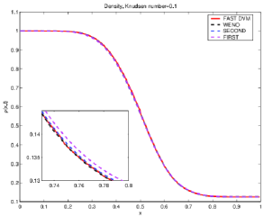
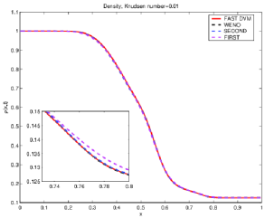
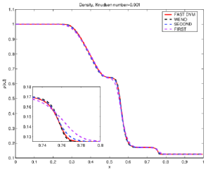
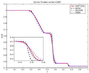
Figure 1: Sod test: solution at $t_{\text{final}}=0.05$ for the density, with $\tau=10^{-1}$ (top left), $\tau=10^{-2}$ (top right), $\tau=10^{-3}$ (bottom left) and $\tau=10^{-4}$ (bottom right).

In this section, we present several numerical tests to illustrate the main features of the method. First the performance of the scheme is tested in the one dimensional case for solving the Sod problem. In this case, we do comparisons of our method with different finite difference methods which can solve the same problem. In the one dimensional case, the computational speedup is not very relevant being all classical methods sufficiently fast. However, the FKS method is still faster than the other methods. In a second series of tests we solve a two dimensional- two dimensional kinetic equation. Finally we solve a full three-three dimensional problem. In this situation, it is a matter of fact that computing the solution of a kinetic equation with finite difference, finite volume or semi-Lagrangian methods is unreasonable. We will show results from our method running on a mono-processor laptop machine.

6.2 1D Sod shock tube problem

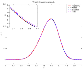
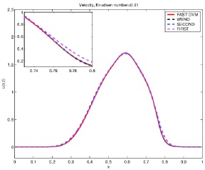
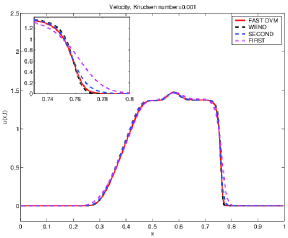
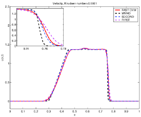
Figure 2: 1D Sod test: solution at $t_{\text{final}}=0.05$ for the mean velocity, with $\tau=10^{-1}$ (top left), $\tau=10^{-2}$ (top right), $\tau=10^{-3}$ (bottom left) and $\tau=10^{-4}$ (bottom right).

We consider the 1D/1D Sod test with $300$ mesh points in physical and $100$ points in velocity spaces. The boundaries in velocity space are set to $-15$ and $15$. The left and right states are given by a density $\rho_{L}=1$, mean velocity $u_{L}=0$ and temperature $T_{L}=5$ if $0\leq x\leq 0.5$, while $\rho_{R}=0.125$, $u_{R}=0$, $T_{R}=4$ if $0.5\leq x\leq 1$. The gas is in thermodynamical equilibrium. We repeat the same test with $4$ different values of the Knudsen number, ranging from $\tau=10^{-1}$ to $\tau=10^{-4}$. We plot the results for the final time $t_{\text{final}}=0.05$ for the density (Figure 1), the mean velocity (Figure 2) and the temperature (figure 3). In each figure we compare the FKS method with a third order WENO method, a second-order MUSCL method and a first-order upwind method [23]. These numerical methods used as reference, employ the same discretization parameters, except for the time step which for stability reason is chosen equal to $\Delta t/2$ for the WENO and second-order MUSCL schemes, where $\Delta t$ is the time step of the fast DVM method given by (48).

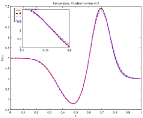
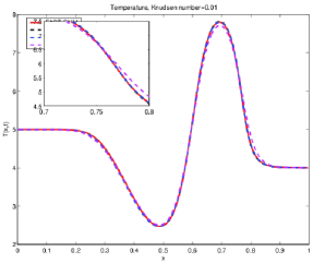
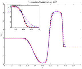
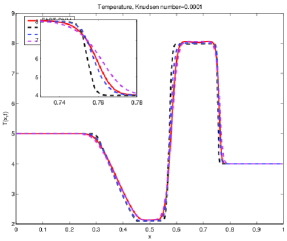
Figure 3: 1D Sod test: solution at $t_{\text{final}}=0.05$ for the temperature, with $\tau=10^{-1}$ (top left), $\tau=10^{-2}$ (top right), $\tau=10^{-3}$ (bottom left) and $\tau=10^{-4}$ (bottom right).

From Figures (1) to (3) we can observe that our method gives very similar results to the two high order schemes for $\tau=10^{-1}$, $\tau=10^{-2}$ and $\tau=10^{-3}$ while for $\tau=10^{-4}$, the scheme is more diffusive than the second and third order scheme but it still performs better than the first order method. The behaviors of the method for different regimes are due to the fact that for collisionless regimes the FKS gives almost the exact solution, this means that it is more precise than the third and second-order methods. When the gas becomes denser the projection towards the equilibrium, which is only first-order (second step of the method (44)), does reduce the accuracy of the method. Notice that high order reconstruction of the equilibrium distribution could also be considered to increase the global accuracy in such case. However, a key point of the FKS is its low CPU time consumption in comparison to other existing methods. In the case $\tau=10^{-4}$ for which the scheme exhibits diffusive behaviors, a comparison between the third order WENO method and our FKS method is carried out for a fixed CPU time. In other words, we consider for a given total computational time, which method gives better results. Thus, we solve the problem with $200$ points in space and $100$ in velocity space for the WENO method and we consider an FKS solver which employs $100$ points in velocity space. In order to have the same computational time for the two methods, we can afford $1000$ points for the FKS. The two results are compared in Figure 4. We observe that, in this situation, the FKS method gives more accurate solutions, in particular for the shock wave (see the zooms in the figures). Finally, observe that the gain in term of computational time is not so relevant for the one dimensional case, while it becomes very important for the two and the three dimensional case. In the later case, the difference is about being able to do or not to do the computation in a reasonable amount of time on a single processor machine.

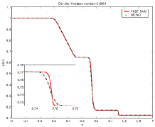
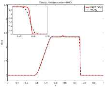
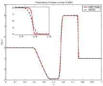
Figure 4: 1D Sod test: solution at $t_{\text{final}}=0.05$ for the density, the mean velocity and the temperature with $\tau=10^{-4}$. Comparison of solutions for the same computational time and different meshes. WENO $200$ points (dashed line) and Fast DVM $1000$ points (straight line).

6.3 2D Sod shock tube problem

We consider now the 2D/2D Sod test on a square $[0,2]\times[0,1]$. The velocity space is also a square with bounds $-15$ and $15$, i.e. $[-15,15]^{2}$, discretized with $N_{v}=20$ points in each direction which gives $20^{2}$ points. We repeat the same test using different $N_{x}\times N_{y}$ meshes ranging from $N_{x}=N_{y}=25$ to $N_{x}=N_{y}=200$. The domain is divided into two parts, a disk centered at point $(1,1)$ of radius $R_{d}=0.2$ is filled with a gas with density $\rho_{L}=1$, mean velocity $u_{L}=0$ and temperature $T_{L}=5$, whereas the gas in the rest of the domain is initiated with $\rho_{R}=0.125$, $u_{R}=0$, $T_{R}=4$. The final time is $t_{\text{final}}=0.07$. The gas is in thermodynamical equilibrium during all the computation which means that we fix $\tau=0$. In practice, we are using the kinetic scheme to compute the solution of the compressible Euler equation. We recall that, as seen in the previous section, this is the case in which the FKS scheme gives the worse results, this is due to the first order accurate projection towards the local Maxwellian distribution. However, this choice permits to compare our results with a numerical method for the compressible Euler equations, being as already stated, computationally very demanding to perform simulations of kinetic equations in the two dimensional case and considerably more demanding in the three dimensional case.

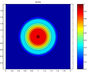
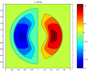
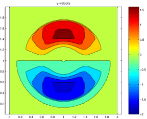
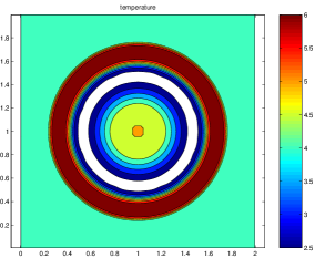
Figure 5: 2D Sod test: solution at $t_{\text{final}}=0.07$ for the density (top left), the velocity in the x-direction (top right), the velocity in the y-direction (bottom left) and the temperature (bottom right).

In Figure 5 we show the results for respectively the density, the mean velocity in the $x$-direction and in the $y$-direction and the temperature using a $200\times 200$ mesh. In Figure 6 we report the profile for $x=1$ of the same macroscopic quantities comparing the results to a first order and to a second order MUSCL scheme for the compressible Euler equations [23]. We clearly see that, as in the 1D case, the accuracy of the FKS method lies between the first and the second order accuracy in the limit $\tau\rightarrow 0$. We expect the accuracy to be highly improved when the gas is far from the thermodynamical equilibrium as in the one dimensional case.

In table 1 we report the CPU time $T$ of these simulations, the CPU time per time cycle $T_{\text{cycle}}$, the CPU time per cycle per cell $T_{\text{cell}}$ and the number of cycles needed to perform the computation for different meshes in space and a fixed mesh in velocity. As expected the number of time step linearly scales with the size of the spatial mesh at fixed velocity mesh (factor $2$ when the cell number is multiplies by $4$). The CPU time is very small compared to classical kinetic schemes, in less than $10$ minutes the simulation of the Sod shock tube on a $200$ mesh is computed. Finally we observe that the CPU time per cycle per cell is almost constant which allows to predict the end of the simulation and its cost beforehand.

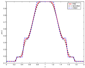
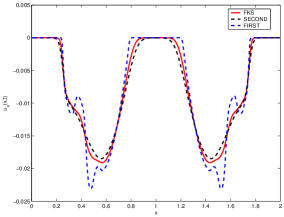
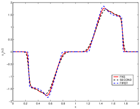
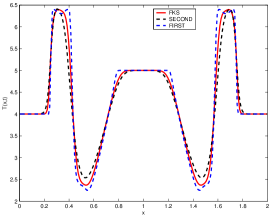
Figure 6: 2D Sod test: solution (continuous line) at $t_{\text{final}}=0.07$ and $x=1$ for the density (top left), the velocity in the x-direction (top right), the velocity in the y-direction (bottom left) and the temperature (bottom right). Comparisons with first order and second order MUSCL methods (dotted lines)

6.4 Numerical validation of the 3D/3D fast FKS method

Here we report some simulations of the full 3D/3D problem. We consider only the case in which $\tau\equiv 0$, which means, we project towards equilibrium at each time step, this is the fluid limit. We recall that, in this regime, the numerical method gives the worst results in terms of precision, on the other hand, exact solution are known and this permits to make fair comparisons. For all the other regimes, the performances of the method are better as shown in the previous section.

The FKS method has been implemented in fortran on a sequential machine. The goal is to numerically show that such a kinetic scheme can reasonably perform on six dimensions on a mono-processor laptop. All simulations have been carried out on a HP EliteBook 8740W Intel(R) Core(TM) i7 Q840@1.87GHz running under a Ubuntu (oneiric) version 11.10. The code has been compiled with gfortran 4.6 compiler with -O3 optimization flags.

Otherwise noticed the velocity space is $[-15,15]^{3}$ or $[-10,10]^{3}$ and is discretized with $N_{v}=13$ or $N_{v}=12$ grid points in each velocity direction, leading to $N_{v}^{3}=2197$ or $1728$ mesh points. The time step is fixed to $95\%$ of the maximum time step allowed, as prescribed by the CFL condition (48), apart from the last time step which is chosen to exactly match the user-given final time. Symmetric boundary conditions are considered.

The Sod shock tube in 1D is run as a sanity checks in order to validate the implementation of the method and show its ability to reproduce 1D results with a 3D run. Then the Sod problem in 3D is simulated to show the performances of the FKS algorithm and further compared to a reference solution. For each simulation we report the memory consumption, the full CPU time and the CPU time cost per cell per time step. Some extrapolation of these results are also made to measure the efficiency of this method.

6.4.1 1D Sod shock tube problem: A sanity check

Cell v #		Cell x # $N_{c}$	Cell $x\times v$ # $N_{tot}$	Cycle	Time	Time/cycle	Time/cell
$N^{2}_{v}$	Bounds	$N_{x}\times N_{y}$	$N_{x}\times N_{y}\times K^{2}$	$N_{\text{cycle}}$	T (s)	$T_{\text{cycle}}$ (s)	$T_{\text{cell}}$ (s)
		$25\times 25$	$25\times 25\times 20^{2}$	$13$	$2$s	$0.1538$	$2.46\times 10^{-4}$
		$=625$	$=250000$
$20^{2}$	$[-15,15]$	$50\times 50$	$50\times 50\times 20^{2}$	$25$	$8$s	$0.32$	$1.28\times 10^{-4}$
		$=2500$	$=10^{6}$
		$100\times 100$	$100\times 100\times 20^{2}$	$50$	$60$s	$1.2$	$1.20\times 10^{-4}$
		$=10000$	$=4\ 10^{6}$		$1$mn
		$200\times 200$	$200\times 200\times 20^{2}$	$100$	$490$s	$535.75$	$1.22\times 10^{-4}$
		$=40000$	$=16\ 10^{6}$		$\sim 8$mn

Table 1: 2D Sod shock tube. The time per cycle is obtained by $T_{\text{cycle}}=\text{T}/N_{\text{cycle}}$ and the time per cycle per cell by $T_{\text{cell}}=\text{T}/N_{\text{cycle}}/N_{c}$.

The first sanity check consists of running the 1D Sod shock tube in $x$ direction on $N_{x}\times 2\times 2$ cubes. The initial data are the same as for the 1D problem previously run. The final time is $t_{\text{final}}=0.1$. In our numerical experiments the computational domain is of size $1$ in $x$ direction leading to $\Delta x=1/N_{x}$. We set $\Delta y=\Delta z=\Delta x$. Four successively refined meshes in $x$ direction are utilized, $N_{x}=50,100$, $200$, and $400$, in order to observe the convergence of the numerical method towards the exact solution.

In Figure 7 we display the density, the velocity and the temperature vs the exact solution with solid line (respectively panels (a), (c) and (d)) and a 3D view on the mesh cells colored by density (panel (b) where a $200\times 3\times 3$ mesh is used for figure scaling reasons). The first observation is the perfect symmetry in the ignorable directions $y$ and $z$ as all cells are plotted (notice that the results for a $N_{x}\times 5\times 5$ cells mesh exactly match the $N_{x}\times 2\times 2$ results). The second obvious observation is the convergence of the numerical solution towards the exact solution when the mesh is refined. These results assess the ability of the method and the code to reproduce 1D results without alteration.

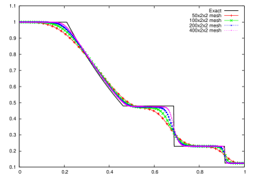
(a)	(b)
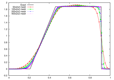
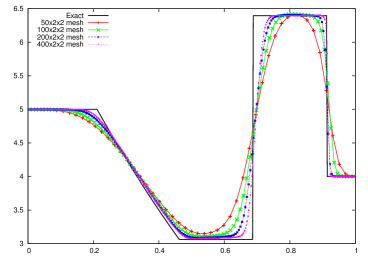
(c)	(d)

Figure 7: 3D-1D Sod problem at $t_{\text{final}}=0.1$ for $50,100$, $200$, and $400$ cells in $x$ direction and $2$ in $y$ and $z$ directions — Panels (a), (c), (d): Density, velocity and temperature as a function of $x$ vs exact solution (straight line) — Panel (b): 3D view of colored density for a $200\times 3\times 3$ mesh.

In table 2 we gather the number of cycles $N_{\text{cycle}}$, the CPU time $T$ of these simulations and display the CPU time per time cycle $T_{\text{cycle}}$ and the CPU time per cycle per cell $T_{\text{cell}}$. As expected, the cycle number and the CPU time per time cycle scales with the cell number and, consequently, the CPU time per cycle per cell is almost constant. This allows to almost exactly predict the duration of a simulation knowing the cell number. Moreover we have provided the relative percentage of the cost of the transport and collision stages.

As expected the transport stage does not cost anything, in absolute value, especially when the number of cells increases. In fact, for computing the solution of this stage in all domain, we consider the evolution of the distribution function $f$ in one single cell, the same happens in the other cells. This means that the cost of this stage is proportional to the $N_{v}^{3}$ mesh points in the velocity space. On the other hand, in finite volume methods as well as Monte Carlo method the cost to solve this stage is proportional to $N_{v}^{3}N_{c}$ with $N_{c}=N_{x}N_{y}N_{z}$ and, obviously this scales with $N_{c}$. Another satisfactory result is the memory storage $Mem$ in MB (or Mo) of the method which is very low because we never have to store the distribution function values for more than $N_{v}^{3}$ points, leading to store $13^{3}\times 7$ reals, say $\sim 0.123$MB independently of $N_{c}$. Conversely the storage of the Monte Carlo method scales with the cell number $N_{c}$. Finally as expected the time T scales with a factor $4$ for twice the number of cells.

Cell #	Cycle	Time	Time/cycle		Time/cycle/cell	Memory
$N_{x}\times N_{y}\times N_{z}\times N^{3}_{v}$	$N_{\text{cycle}}$	$T$(s)	$T_{\text{cycle}}$(s)		$T_{\text{cell}}$(s)	Mem(MB)
$=N_{c}\times N^{3}_{v}$			Transp.	Coll.
$50\times 2\times 2$	$81$	$18$	$0.22$		$1.11\times 10^{-3}$	$0.660$
$=200\times 13^{3}=439400$			$0.07\%$	$99.93\%$
$100\times 2\times 2$	$160$	$68$	$0.43$		$1.07\times 10^{-3}$	$0.704$
$=400\times 13^{3}=878800$			$0.05\%$	$99.95\%$
$200\times 2\times 2$	$318$	$276$	$0.87$		$1.08\times 10^{-3}$	$0.812$
$=800\times 13^{3}=1757600$			$0.03\%$	$99.97\%$
$400\times 2\times 2$	$634$	$1071$	$1.69$		$1.06\times 10^{-3}$	$1.000$
$=1600\times 13^{3}=3515200$			$0.02\%$	$99.98\%$

Table 2: 1D Sod shock tube run with the 3D/3D FKS method. The time per cycle is obtained by $T_{\text{cycle}}=\text{T}/N_{\text{cycle}}$ and the time per cycle per cell by $T_{\text{cell}}=\text{T}/N_{\text{cycle}}/N_{c}$. The relative percentage of the cost of the transport and relaxation stages are provided. For our FKS method the transport stage costs almost nothing.

6.4.2 3D Sod shock tube problem

The 3D Sod shock tube has been run with the 3D/3D FKS method. The left state of the 1D Sod problem is set for any cell $c$ with cell center radius $r_{c}\leq 1/2$, conversely the right state is set for cell radius $r_{c}>1/2$. The final time is $t_{\text{final}}=0.1$. The domain is the unit cube and the mesh is composed of $N_{x}\times N_{x}\times N_{x}$ cells with $\Delta x=1/N_{x}$ and $\Delta x=\Delta y=\Delta z$. The problem is run with $N_{x}=50$ ($125000$ cells), $N_{x}=100$ ($1$ million cells) and $N_{x}=200$ ($8$ millions cells). The velocity space is either $[-10;10]$ discretized with $12^{3}$ points, or $[-15;15]$ discretized with $13^{3}$ points. This leads to consider up to $200^{3}\times 13^{3}\simeq 17.7$ milliards cells. In Figure 8 the density is plotted as a function of the radius (left panel) and the colored density on a 3D view (right panel) for $N_{x}=50$ (middle panels) and $N_{x}=200$ (bottom panels). The two different choices for the bounds and the mesh points in velocity space do not significantly change the results hence only the solution with bounds $[-10;10]$ and with $12^{3}$ mesh points is reported. The reference solution is obtained with a 2D axisymmetric compatible staggered Arbitrary-Lagrangian-Eulerian code [25] with $1000$ cells in radial and $20$ cells in angular directions.

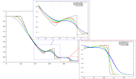
Figure 8: Sod problem at $t_{\text{final}}=0.1$ for $N_{x}\times N_{x}\times N_{x}$ cells (for $N_{x}=50,100,200$) for the velocity space $[-10;10]$ discretized with $12^{3}$ mesh points. — Top: Convergence of density as a function of cell center radius for all cells vs converged solution (straight thick line) for the three meshes with zooms on contact and shock waves. Left: Density as a function of cell center radius (middle: $N_{x}=50$, bottom: $N_{x}=200$) Right: 3D view of density on the unit cube $N_{x}=50$ (middle) and $N_{x}=200$ (bottom) (the mesh is only shown for $N_{x}=50$).

Moreover in Figure 8 (top panel) we present the convergence of the density as a function of cell center radius for all cells for the $50\times 50\times 50$, $100\times 100\times 100$ and $200\times 200\times 200$ cells meshes. These curves are compared to the reference solution in straight thick line and they show that the results are converging towards the reference solution. In table 3 we gather the number of time steps and the total CPU time T for $50^{3}$ and $100^{3}$ cell meshes for the two different configurations: one with $N_{v}=13$ and the velocity space $[-15,15]$ and the second one with $N_{v}=12$ and the velocity space $[-10,10]$. For the $50^{3}$ mesh the simulation takes $45$ minutes or $1.36$ hour depending on the configuration. For the finer $100^{3}$ mesh the simulation takes either $11$ hours or $24$ hours The memory consumption ranges from $124$Mb to $924$Mb depending on the configurations and it scales with the number of cells $N_{c}$.

Then, we compute the cost per cycle $T_{\text{cycle}}$ and per cycle per cell $T_{\text{cell}}$. One observe that the cost per cycle per cell is an almost constant equal to $4\times 10^{-4}$s or $5.5\times 10^{-4}$s. The extrapolation of the CPU time $T$ for a $200^{3}$ mesh at $T_{\text{cell}}$ fixed leads to one or two weeks computation for the two configurations and a memory storage of about $900$MB.

		Cell # $N_{c}\times N_{v}^{3}$	Cycle	Time	Time/cycle	Time/cell	Mem
$N^{3}_{v}$	Bounds	$N_{x}\times N_{y}\times N_{z}\times N_{v}^{3}$	$N_{\text{cycle}}$	T (s)	$T_{\text{cycle}}$ (s)	$T_{\text{cell}}$ (s)	(MB)
$13^{3}$	$[-15,15]$	$25^{3}\times 13^{3}$	$32$	$346$s	$10.81$	$6.92\times 10^{-4}$	$2.4$
		$=3.4328125\times 10^{6}$		($5.76$mn)
		$50^{3}\times 13^{3}$	$81$	$4900$s	$60.50$	$4.84\times 10^{-4}$	$15.5$
		$=274.625000\times 10^{6}$		($1.36$h)
		$100\times 13^{3}$	$160$	$85720$s	$535.75$	$5.36\times 10^{-4}$	$115.5$
		$=2.1970\times 10^{9}$		($23.8$h)
extrapol.		$200\times 13^{3}$	$320$	$\sim 1.4\times 10^{6}$s	$\sim 4400$	$5.5\times 10^{-4}$	$\sim 900$
		$=1.7576\times 10^{10}$		($16$d)
$12^{3}$	$[-10,10]$	$25^{3}\times 12^{3}$	$27$	$218$s	$8.07$	$5.17\times 10^{-4}$	$2.3$
		$=27\times 10^{6}$		($3.63$mn)
		$50^{3}\times 12^{3}$	$54$	$2702$s	$50.03$	$4.00\times 10^{-4}$	$15.4$
		$=125\times 10^{3}$		($45$mn)
		$100^{3}\times 12^{3}$	$107$	$38069$s	$355.79$	$3.56\times 10^{-4}$	$115.4$
		$=1.728\times 10^{9}$		($10.57$h)
extrapol.		$200^{3}\times 12^{3}$	$214$	$\sim 633440$s	$\sim 2960$	$3.7\times 10^{-4}$	$\sim 900$
		$=1.3284\times 10^{10}$		($7$d)

Table 3: 3D Sod shock tube. The time per cycle is obtained by $T_{\text{cycle}}=\text{T}/N_{\text{cycle}}$ and the time per cycle per cell by $T_{\text{cell}}=\text{T}/N_{\text{cycle}}/N_{c}$. The lines marked with extrapol. have been extrapolated by fixing $N_{c}$, $N_{\text{cycle}}$ and $T_{\text{cell}}$.

In Figure 9 we plot the CPU time (red or blue symbols for each configuration and mesh points of the velocity space) and the extrapolation curves $CPU(N_{x},N_{c},T_{\text{cell}})=\frac{N_{\text{cycle}}}{N_{x}}N_{c}T_{\text{cell}}$ for the 3D Sod problem up to time $t_{\text{final}}=0.1$ for single processor laptop computation on a fixed mesh in velocity space of $N_{v}=12^{3}$ points. We deduced that the FKS method can be used at most on a single processor machine up to a $200\times 200\times 200$ cells for roughly one week of computation. One also notices that the CPU time linearly scales on a log/log graph as expected (right panel of Figure 9)

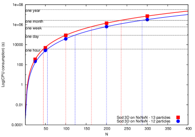
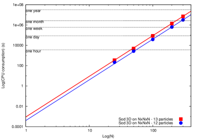
Figure 9: Left: Log of the CPU time consumption for the 3D Sod problem at $t_{\text{final}}=0.1$ as a function of $N$ (for $N\times N\times N$ cell meshes) on a single processor laptop The red/blue squares are taken from Table 3, the thick red/blue curves are the extrapolation curve from $T_{\text{cell}}$. The horizontal lines corresponding to one hour, one day, week, month and year are also plotted. $N=100$ corresponds to the ’one million cells’ in space — Right: Log/Log scale.

7 Conclusions

In this work we have presented a new super efficient numerical method for solving kinetic equations. The method is based on a splitting between the collision and the transport terms. The collision part is solved on a grid while the transport linear part is solved exactly by following the characteristics backward in time. The key point is that, conversely to semi-Lagrangian methods, we do not need to reconstruct the distribution function at each time step. In this first paper, we have presented the basic formulation of this new method for the BGK equation: Uniform meshes, piecewise constant discretization of the velocity space and a simple projection towards the equilibrium distribution have been considered.

The numerical results show that the method is incredibly fast. We are now able to perform numerical simulations of the full six dimensional kinetic equation on a single processor machine in several hours. This important result opens the gate to extensive realistic numerical simulations of far from equilibrium physical models. Concerning the precision of the method, we observed, as expected, that the fast kinetic scheme (FKS) is more dissipative close to the fluid regime and very precise for gases far from the thermodynamical equilibrium.

In the future we would like to extend the method to non uniform meshes, more advanced boundary conditions and different discretization of the velocity space. One expects with this last point to increase the accuracy of the schemes without losing its attractive efficiency. To avoid the loss of accuracy close to the fluid limit, we want to couple the FKS method to an high order solver for the system of equations which describes the fluid limit. Finally, we want to extend the method to other kinetic equations as the Boltzmann or the Vlasov equation.

References

- [1] G.A.Bird, Molecular gas dynamics and direct simulation of gas flows, Clarendon Press, Oxford (1994).
- [2] C.K. Birsdall, A.B. Langdon, Plasma Physics Via Computer Simulation, Institute of Physics (IOP), Series in Plasma Physics (2004).
- [3] A.V. Bobylev, A. Palczewski, J. Schneider, On approximation of the Boltzmann equation by discrete velocity models. C. R. Acad. Sci. Paris Ser. I. Math. 320, (1995), pp. 639-644.
- [4] J. Burt, I. Boyd, A low diffusion particle method for simulating compressible inviscid flows, J. Comput. Phys., Vol. 227, (2008), pp. 4653–4670
- [5] R. E. Caflisch, Monte Carlo and Quasi-Monte Carlo Methods, Acta Numerica, (1998), pp. 1–49.
- [6] R. E. Caflisch, L. Pareschi, Towards an hybrid method for rarefied gas dynamics, IMA Vol. App. Math., vol. 135 (2004), pp. 57–73.
- [7] C. Cercignani, The Boltzmann Equation and Its Applications, Springer-Verlag, New York, (1988).
- [8] N. Crouseilles, T. Respaud, E. Sonnendrücker, A Forward semi-Lagrangian Method for the Numerical Solution of the Vlasov Equation, Comp. Phys. Comm. 180, 10 (2009) 1730–1745.
- [9] N. Crouseilles, M. Mehrenberger, E. Sonnendrücker, Conservative semi-Lagrangian schemes for Vlasov equations, J. Comp. Phys., (2010) pp. 1927–1953.
- [10] L. Desvillettes, S. Mischler, About the splitting algorithm for Boltzmann and BGK equations. Math. Mod. & Meth. in App. Sci. bf 6, (1996), pp. 1079–1101.
- [11] P. Degond, S. Mas-Gallic, The weighted particle method for convection-diffusion equations. II. The anisotropic case, Math. Comp. Vol. 53 (1989), pp. 509 525.
- [12] P. Degond, G. Dimarco, L. Pareschi, The Moment Guided Monte Carlo Method, Int. J. Num. Meth. Fluids, Vol.67, (2011), pp. 189–213.
- [13] P. Degond, J.-G. Liu, L. Mieussens, Macroscopic fluid models with localized kinetic upscaling effects, SIAM MMS, vol. 5 (2006), pp. 940–979.
- [14] G. Dimarco, L. Pareschi, A Fluid Solver Independent Hybrid method for Multiscale Kinetic Equations, SIAM J. Sci. Comput. Vol. 32, (2010), pp. 603–634.
- [15] G. Dimarco, L. Pareschi, Hybrid multiscale methods II. Kinetic equations, SIAM Mult. Model. and Simul. Vol 6., (2007), pp. 1169–1197.
- [16] W. E, B. Engquist, The heterogeneous multiscale methods, Comm. Math. Sci., vol. 1 (2003), pp. 87-133.
- [17] F. Filbet, G. Russo, High order numerical methods for the space non-homogeneous Boltzmann equation. J. Comput. Phys., 186 (2003), 457–480.
- [18] F. Filbet, E. Sonnendrücker, P. Bertrand, Conservative Numerical schemes for the Vlasov equation. J. Comput. Phys. 172, (2001) pp. 166–187.
- [19] I.M. Gamba, S. H. Tharkabhushaman, Spectral - Lagrangian based methods applied to computation of Non - Equilibrium Statistical States. J. Comput. Phys. 228, (2009) pp. 2012–2036.
- [20] E.P. Gross P.L. Bathnagar, M. Krook, A model for collision processes in gases. I. small amplitude processes in charged and neutral one-component systems Phys. Rev. 94 (1954), pp. 511–525.
- [21] T. Homolle, N. Hadjiconstantinou, A low-variance deviational simulation Monte Carlo for the Boltzmann equation. J. Comput. Phys., Vol 226 (2007), pp 2341–2358.
- [22] T. Homolle, N. Hadjiconstantinou, Low-variance deviational simulation Monte Carlo. Phys. Fluids, Vol 19 (2007), 041701.
- [23] R. J. LeVeque, Numerical Methods for Conservation Laws, Lectures in Mathematics, Birkhauser Verlag, Basel (1992).
- [24] S. Liu, Monte Carlo strategies in scientific computing, Springer, (2004).
- [25] R. Loubère, First steps into ALE INC(ubator). A 2D arbitrary-lagrangian-eulerian code on general polygonal mesh for compressible flows - Version 1.0.0, Los Alamos National Laboratory Report, LA-UR-04-8840, (2004).
- [26] S. Mas-Gallic, A deterministic particle method for the linearized Boltzmann equation, Transp. Theory Stat. Phys., Vol. 16, (1987), pp. 885-887.
- [27] S. Mas-Gallic, F. Popaud, Approximation of the transport equation by a weighted particle method, Transp. Theory Stat. Phys., Vol. 17, (1988), pp. 311-345
- [28] L. Mieussens, Discrete Velocity Model and Implicit Scheme for the BGK Equation of Rarefied Gas Dynamic, Math. Models Meth. App. Sci., Vol. 10, (2000), 1121–1149.
- [29] K. Nanbu, Direct simulation scheme derived from the Boltzmann equation, J. Phys. Soc. Japan, vol. 49 (1980), pp. 2042–2049.
- [30] W.F. Noh, Errors for calculations of strong shocks using an artificial viscosity and an artificial heat flux., J. Comput. Phys. 72, (1987), pp 78-120
- [31] A. Palczewski, J. Schneider, A.V. Bobylev, A consistency result for a discrete-velocity model of the Boltzmann equation. SIAM J. Numer. Anal. 34, (1997) pp. 18651883.
- [32] A. Palczewski, J. Schneider, Existence, stability, and convergence of solutions of discrete velocity models to the Boltzmann equation. J. Statist. Phys. 91, (1998) pp. 307326.
- [33] L. Pareschi, G. Russo, Time Relaxed Monte Carlo methods for the Boltzmann equation, SIAM J. Sci. Comput. 23 (2001), pp. 1253–1273.
- [34] L. Pareschi, Hybrid multiscale methods for hyperbolic and kinetic problems, Esaim Proceedings, Vol. 15, T. Goudon, E. Sonnendrucker & D. Talay Editors (2005), pp.87-120.
- [35] S. Pieraccini, G. Puppo, Implicit-explicit schemes for BGK kinetic equations, J. Sci. Comp. (2007), pp. 1-28.
- [36] D. I. Pullin, Direct simulation methods for compressible inviscid ideal gas flow, J. Comput. Phys., 34 (1980), pp. 231–244.
- [37] G. Strang, On the construction and the comparison of difference schemes. SIAM J. Numer. Anal., (1968), pp. 506–517.