A general existence theorem for embedded minimal surfaces with free boundary
Abstract.
In this paper, we prove a general existence theorem for properly embedded minimal surfaces with free boundary in any compact Riemannian 3-manifold with boundary . These minimal surfaces are either disjoint from or meet orthogonally. The main feature of our result is that there is no assumptions on the curvature of or convexity of . We prove the boundary regularity of the minimal surfaces at their free boundaries. Furthermore, we define a topological invariant, the filling genus, for compact 3-manifolds with boundary and show that we can bound the genus of the minimal surface constructed above in terms of the filling genus of the ambient manifold . Our proof employs a variant of the min-max construction used by Colding and De Lellis on closed embedded minimal surfaces, which were first developed by Almgren and Pitts.
1. Background and motivation
In this paper, we study a general existence problem for embedded minimal surfaces with free boundary. All manifolds (with or without boundary) are assumed to be smooth up to the boundary unless otherwise stated.
Question 1.
Given a compact Riemannian three-manifold with boundary , does there exist a properly embedded minimal surface with boundary such that meets orthogonally along ?
Recall that a surface (with or without boundary) is said to be properly embedded if the inclusion map is a proper embedding (i.e. a one-to-one immersion). In other words, we require
-
(i)
; and
-
(ii)
is transversal to at any point on .
Note that if , this is equivalent to saying that is contained in the interior of .
The orthogonality condition along the boundary is a natural condition arising variationally. Let be a properly embedded surface with boundary . Suppose we have a smooth family of properly embedded surfaces in for some with . If we calculate how the area of this family of surfaces, denoted by Area(), changes with respect to at , a standard computation (for example, see [35] and [36]) gives the first variation formula
| (1.1) |
where is the metric of the ambient manifold , is the outer conormal vector of in (i.e. the outward unit normal of tangent to ), is the mean curvature vector of in (with the sign convention that points inward for the unit sphere in ) and is the variation field associated with the one-parameter family (i.e. where is a one-parameter family of proper embeddings such that ). Note that since for all , the variation field is tangential to along . From (1.1), is a critical point to the variational problem if and only if is minimal (i.e. ) and meets orthogonally along (i.e. ). In this case, we say that is a free boundary solution.
The study of free boundary problems for minimal surfaces was initiated by R. Courant in [6] and H. Lewy in [21] in the 1940’s. In the next few decades, these minimal surfaces with free boundaries were studied extensively by K. Goldhorn, S. Hildebrandt, W. Jäger and J. Nitsche (see, for example, [16] [27] [28] [12] [17] [15]), and later by J. Taylor [39], W. Meeks and S.T. Yau [25], and R.Ye [41], among many others. In their approaches, they applied the direct method in the calculus of variations to the Dirichlet energy functional, and established the existence of minimizers with boundary lying on a given supporting surface. Boundary regularity results were obtained in a variety of settings. Interested readers are encouraged to consult the recent treatise [8] [9] on boundary value problems of minimal surfaces.
However, this approach cannot be used directly to answer Question 1. The main reason is that these existence theorems only produce area minimizers, they do not yield the existence of stationary minimal surfaces which are not area minimizing. It is not hard to see that for certain supporting surfaces, there are no non-trivial minimizers. For example, it does not furnish the existence of non-trivial stationary minimal surfaces within the region bounded by a closed convex surface in . Therefore, the direct method does not work unless the ambient space has some non-trivial topology.
To deal with the difficulty above, we need to construct unstable critical points to the area (or energy) functional. Along this direction, M. Struwe [38] and A. Fraser [10] applied the celebrated perturbed -energy of Sacks and Uhlenbeck [32] to the free boundary problem for minimal disks. They were able to produce non-trivial free boundary solutions with controlled Morse index using Ljusternik-Schnirelman theory. For instance, A. Fraser proved that (see Theorem 1 in [10]) if is a smooth compact domain of a complete, homogeneously regular Riemannian three-manifold , and the relative homotopy group for some , then either there exists a non-constant minimal disk in meeting orthogonally along , or there exists a non-constant minimal two-sphere in . Moreover, the Morse index of such a minimal surface is at most .
Despite these positive results in the existence theory, it is yet not enough to settle Question 1 in complete generality due to the following reasons. First, the minimal disk or sphere may not be embedded (in fact it may not even be immersed). Second, and more importantly, the free boundary solution may not be contained in the compact region . The construction does not prevent the minimal surface from penetrating in an unphysical way, and it is impossible to make it contained in without imposing (mean) convexity assumptions on (see [11] [25] [26]). This approach does not work in the non-convex situation because one do not expect to contain a disk-type free boundary solution. For example, the annular region , where denotes the ball of radius centered at the origin, does not contain any properly embedded minimal disk with free boundary on . If such a minimal disk were to exist, the boundary circle lies on one of the boundary spheres or . It cannot lie on by the convex hull property (see Proposition 1.9 in [5]). Therefore, , and hence is a free boundary solution to the ball . A uniqueness theorem of J. Nitsche [29] implies that must be a totally geodesic equatorial disk, which has non-empty intersection with the unit ball , contradicting the hypothesis that . On the other hand, the restriction of the equatorial disk to gives an example of a free boundary solution which is topologically an annulus (genus zero with two boundary components).
There is a completely different approach, using geometric measure theory, which has been very successful in constructing embedded minimal surfaces. By minimizing among all embedded disks with prescribed boundary, F. Almgren and L. Simon [2] showed that any extremal curve in , i.e. is contained in the boundary of a strictly convex domain , bounds an embedded minimal disk contained in . Based on Almgren and Simon’s paper, W. Meeks, L. Simon and S.T. Yau [24] proved, under suitable hypothesis, the existence of an embedded minimal surface which minimizes area in its isotopy class in a Riemannian 3-manifold. This result has profound applications in 3-manifold topology.
In a remarkable work of F. Almgren [20] and J. Pitts [30], a minimax argument was used to prove that any closed Riemannian 3-manifold contains a smooth, embedded, closed minimal surface. The proof of interior regularity for such minimal surfaces was based on Schoen, Simon and Yau’s curvature estimates for stable minimal surfaces [33]. Using a clever curve lifting argument, L. Simon and F. Smith [37] were able to control the topology of the minimal surface. As a corollary, they proved that there exists an embedded minimal two-sphere in the three-sphere with arbitrary Riemannian metric.
Adapting these ideas to the free boundary case, M. Grüter and J. Jost [13] proved the existence of an embedded minimal disk as a free boundary solution in any bounded, strictly convex domain in . In another paper [19], J. Jost claimed similar results hold under weaker convexity assumptions on the boundary. Unfortunately, the author was unable to verify some of the arguments in the paper. On the other hand, a partially free boundary problem was also studied by J. Jost in [18]. All of these results depend on certain curvature assumptions on the boundary of the ambient manifold.
In this paper, we settle Question 1 in complete generality, without any curvature assumptions on or .
Theorem 1.1.
For any compact Riemannian three-manifold with boundary , at least one of the following holds:
-
(i)
there exists a properly embedded minimal surface with boundary such that meets orthogonally along ; or
-
(ii)
there is a closed, embedded minimal surface contained in the interior of .
Moreover, if is assumed to be smooth up to the boundary, then the minimal surface is smooth (up to the boundary in case (i)).
The proof of Theorem 1.1 employs a minimax construction similar to the one by F. Almgren [20] and J. Pitts [30]. Recently, T. Colding and C. De Lellis [4] wrote a detailed account of the minimax construction, and they were able to simplify some of the proofs significantly. In another recent paper [7], C. De Lellis and F. Pellandini obtained a genus bound for minimal surfaces constructed by the minimax method in [4]. (Their bound is slightly weaker than the one conjectured by J. Pitts and H. Rubinstein [31].) We observe that their result can be used to control the topology of the free boundary solution constructed in Theorem 1.1.
Theorem 1.2.
Let be a Riemannian 3-manifold with boundary. Suppose the filling genus (see Definition 9.1) of is equal to . Then, the minimal surface in Theorem 1.1 can be chosen such that
-
(i)
if is orientable, then genus;
-
(ii)
if is non-orientable, then genus.
It is clear from the definition that the filling genus of any compact domain in is zero. As a consequence, we have the following corollary (note that there is no closed minimal surface in ).
Corollary 1.3.
For any compact domain , there exists a properly embedded minimal surface with non-empty free boundary such that either
-
(i)
is orientable with genus zero (i.e. a disk with holes); or
-
(ii)
is a non-orientable surface with genus one (i.e. a Möbius strip with holes).
In case is diffeomorphic to the unit 3-ball, case (ii) does not happen and must be orientable.
The outline of this paper is as follows. In section 2, we describe an example which illustrates why the proof in [4] does not directly generalize to cover the free boundary problem. This example also serves as a model case which motivates many of the technical arguments in this paper. Section 3 to 8 comprise of the proof of our main result, Theorem 1.1. In section 3, we give some definitions and preliminary results. Moreover, we define two important concepts: freely stationary and outer almost minimizing property, which will play important roles in this paper. In section 4, we describe the min-max construction and give an outline of the proof of Theorem 1.1. In section 5 and 6, we establish the existence of varifolds which are both freely stationary and outer almost minimizing. In section 7, we study a minimization problem with partially free boundary, which is then used in section 8 to prove the boundary regularity of freely stationary varifolds satisfying the outer almost minimizing property. In section 9, the genus bound in Theorem 1.2 is proved using the result in [7].
Acknowledgement. The results in this paper form part of the author’s Doctoral Dissertation [22] at Stanford University. The author would like to express his sincere gratitude to his advisor Professor Richard Schoen for suggesting this interesting problem and providing lots of useful advice and support throughout the progress of this work. The author would also like to thank Professor Brian White for many helpful comments and discussions. The author is indebted to Professor Leon Simon, from whom he learned a lot of geometric measure theory used in this paper.
2. An example
In this section, we discuss the main difficulties in the proof of Theorem 1.1. We also give an example which illustrates the need for some technical arguments in this paper.
Our proof of Theorem 1.1 is a modified version of the minimax construction described in [4]. Let us first briefly recall the minimax construction for closed (i.e. compact without boundary) manifolds. Consider the standard 3-sphere (with the round metric, for example), and a continuous sweepout by 2-spheres which degenerate to a point at and . Our goal is to minimize the area of the maximal slice by deforming the sweepout using ambient isotopies (which could depend continuously on ). Suppose a minimizing sweepout exists, we expect a maximal slice in this sweepout to be a minimal surface (see Fig. 2 in [4]). In practice, the minimum may not be achieved by any sweepout. Therefore, we have to take a minimizing sequence of sweepouts, and a min-max sequence of surfaces which, after passing to a subsequence, converges in some weak sense (as varifolds) to an embedded minimal surface (possibly with multiplicity). There are two important points in this construction. First, we need to ensure that almost maximal slices are almost stationary (see Fig. 4 in [4]). This can be achieved by a “tightening” process (section 4 of [4]). Second, we want to choose our min-max sequence carefully so that it satisfies the almost minimizing property which enables us to prove regularity for the limiting surface (sections 5-7 of [4]).
A natural attempt to generalize the above method to the free boundary problem is to sweep out the compact manifold by surfaces with boundary lying on , and we use isotopies which preserve , but not necessarily pointwise fixing points on , to deform our sweepouts. Then, we carry out the same minimax construction as before and hope that a min-max sequence would converge to an embedded minimal surface with free boundary on . In fact, the limit would be stationary with respect to isotopies preserving . Unfortunately, this is insufficient to conclude that the limit is a smooth free boundary solution. The main difficulty is that it may not be properly embedded if we do not have any convexity assumptions on the boundary . Unlike many constructions of minimal surfaces, we do not have barriers to prevent the interior of our minimal surface from touching the boundary. Let us further illustrate this point by the following example.
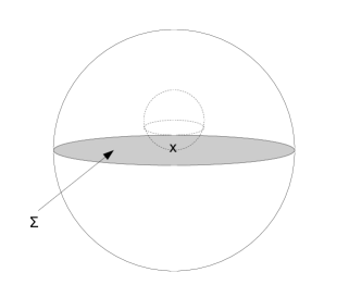
Let be the closed Euclidean 3-ball of radius centered at . Suppose . Consider the equatorial disk , it is minimal and has free boundary on the outer boundary. However, this is not a legitimate free boundary solution because it is not properly embedded. The origin, which lies in the interior of the equatorial disk, is a point on the inner boundary of . This happens since the inner boundary is not mean convex with respect to the inner unit normal (with respect to ). Nevertheless, the equatorial disk is a critical point of the area functional with respect to all variations preserving . Not only is it stationary, but it is also -almost minimizing (see Definition 3.2 in [4]) on any sufficiently small ball for all with respect to these variations. This example shows that a smooth minimal surface which is stationary and almost minimizing with respect to the isotopies preserving may fail to be properly embedded, hence needs not be a free boundary solution (Figure 1). In the next section, we will discuss how to get around this problem.
3. Definitions and preliminaries
Let be a compact Riemannian 3-manifold with non-empty boundary . Suppose is connected (but is not necessary connected, i.e. could have multiple boundary components). Without loss of generality, we assume that is isometrically embedded as a compact subset of a closed Riemannian 3-manifold . (Note that such an isometric embedding always exists. For example, we can smoothly extend with the metric across the boundary to get a collar neighborhood which can be made cylindrical near the boundary by a cutoff function, then we take another copy of this collar neighborhood and glue the two together along the cylindrical necks.) All surfaces, with or without boundary, are smoothly embedded in unless otherwise stated. We will use int to denote the interior of .
3.1. Isotopies and vector fields
We now describe the class of ambient isotopies in used in deforming our surfaces. An isotopy on is a smooth one-parameter family of diffeomorphisms of , where is the identity map of . (The smoothness assumption here means that the map is smooth.) Let denote the space of all isotopies on . Moreover, we say that an isotopy is supported in an open set if for every and . Define
to be the isotopies in which can move points out of the compact set , but not into , and to be those in which are supported in some open set . Furthermore, we are also interested in situations where the compact set is preserved by the isotopy, Similarly, we define
to be the isotopies preserving the compact set , and to be those in supported in some open set . Notice that for any open set .
One way to generate isotopies is to consider the flow of a vector field. Let be the vector space of smooth vector fields on . We define two subspaces and of which correspond to the two classes of isotopies defined above. More precisely, we let
where is the unit outward normal of with respect to and
Notice again that . Each generates a unique isotopy on by its flow (since is closed, the flow exists for all time). Clearly, if , then ; if , then .
3.2. Varifolds and restrictions
Varifolds are fundamental in any min-max construction, compared to other generalized surfaces like currents, because they do not allow for cancellation of mass (see p.24 in [30]). We will discuss some less standard facts about varifolds. For a more comprehensive treatment, one can refer to [1] [4] [23] [36].
Let denote the space of 2-varifolds on endowed with the weak topology (see [36]), and be the subspace of 2-varifolds supported in . There is a restriction map
defined by for any , where and denote the 2-Grassmannian over and respectively. Since is compact, by 2.6.2 (c) in [1], the restriction map is only upper semi-continuous in the weak topology in the following sense: if is a sequence in converging weakly to , then . The following lemma shows that if we have equality , then converges weakly to .
Lemma 3.1.
Let . Suppose is a sequence of varifolds converging weakly to as . If the masses converges to as , then the restricted varifolds converges weakly to as .
The proof of Lemma 3.1 is rather elementary and will be given in Appendix A for the sake of completeness.
3.3. Freely stationary varifolds
Let . If we take a vector field and let be the flow generated by and be the pushforward of by , then is a smooth function in since for all . Differentiating with respect to at , the same calculation as that in the standard first variation formula (see [36] for example) shows that
| (3.1) |
Notice that we are only integrating over instead of on the right hand side of (3.1) since we are only counting area in .
Definition 3.2.
A varifold is said to be freely stationary in an open set if and only if for all vector fields supported in . If , we simply say that is freely stationary.
We denote the set of varifolds which are freely stationary in by and the set of freely stationary varifolds by .
Remark 3.3.
It is obvious that for any and . Therefore, if is freely stationary in , then so is and vice versa. So, we often assume that freely stationary varifolds are supported in .
Using the compactness of mass bounded varifolds in the weak topology and (3.1), it is immediate that the set of mass bounded freely stationary varifolds supported in is compact in the weak topology.
Lemma 3.4.
For any open set , and any constant , the set
is compact in the weak topology.
Proof.
Let be a sequence of varifolds in . Since are supported in , are uniformly bounded by . Therefore, a subsequence of (after relabeling) converges weakly to in by compactness of mass bounded varifolds. Since is a closed subset of , the limit is also supported in , i.e. . Therefore, . It remains to show that is freely stationary in , but this follows directly from the first variation formula (3.1) and the fact that and are supported in . ∎
In this paper, we will use some results in [14], where the monotonicity formula and the Allard regularity for freely stationary varifolds were proved. Their proofs were given for rectifiable varifolds in but they can be easily generalized to general varifolds in Riemannian manifolds. As a result, we have the following monotonicity formula for any freely stationary varifold in : there exists a constant (depending only on the geometry of and ), and a function such that for any and ,
| (3.2) |
Note that goes to as , so the density of the freely stationary varifold at is well-defined.
In [13], the well-known Schoen curvature estimates [34] for stable minimal surfaces were generalized to the free boundary case. The compactness theorem for stable minimal surfaces with free boundary follows easily from the curvature estimates.
Lemma 3.5 (Grüter-Jost [14]).
Let be an open set. Suppose is a sequence of properly embedded stable minimal surfaces in with free boundary on , and their areas are uniformly bounded. Then, for any compact subset , there is a subsequence of converging smoothly (multiplicity allowed) to a properly embedded stable minimal surface in with free boundary lying on .
3.4. Outer almost minimizing property
In general, a stationary varifold may possess singularity and hence is not a smooth minimal surface. Even if it is smooth, the example in section 2 shows that an embedded smooth minimal surface which is freely stationary may fail to be properly embedded. In order to achieve regularity and properness of the freely stationary varifold, we require a stronger condition called outer almost minimizing property. Roughly speaking, a surface is outer almost minimizing means that if you want to decrease its area in through an outward isotopy, its area in must become large at some time during the deformation. The precise definition is given below.
Definition 3.6.
Given and an open set , a varifold is -outer almost minimizing in if and only if there does not exist isotopy such that
-
(1)
for all ;
-
(2)
.
A sequence is said to be an outer almost minimizing sequence in if each is -outer almost minimizing in for some sequence . Moreover, if converges weakly to some in , then we say that is outer almost minimizing in .
Remark 3.7.
The definition is almost the same as the one used in [4] except that we are considering the area in and outward isotopies only.
It is not hard to see that any outer almost minimizing varifold is freely stationary.
Proposition 3.8.
If is outer almost minimizing in , then is freely stationary in .
Proof.
Since is outer almost minimizing in , there exists, by definition, a sequence for which is -outer almost minimizing in . We will prove the proposition by contradiction.
Suppose, in contrary, that is not freely stationary in . Then there is a vector field supported in such that
for some real constant . Let be the flow generated by . Suppose and are the pushforwards of the varifolds and , respectively, by the diffeomorphism . Since , (3.1) implies that is a continuous function in (for fixed). Therefore, we have
| (3.3) |
for all for some . We claim that for all sufficiently large , it holds true that
| (3.4) |
for all .
Let us assume (3.4) for the moment, integrating in gives
| (3.5) |
for all . Since is -outer almost minimizing in , this implies
| (3.6) |
for all sufficiently large. Combining (3.5) and (3.6), we have for sufficiently large. This is a contradiction since .
It remains to verify (3.4). Let and . From the definition of pushforward of a varifold and (3.1), is an equicontinuous family of functions on . Furthermore,
| (3.7) |
for all . Our goal is to prove that for any , for all sufficiently large and all . If not, then there exists a sequence and such that . Without loss of generality, we can assume for some . By equicontinuity, for sufficiently large, we have
Take , we get , which contradicts (3.7). Finally, (3.4) follows from (3.3) by taking .
∎
The example in section 2 shows that the converse of Proposition 3.8 is false (Figure 1). The equatorial disk shown in Figure 1 is freely stationary and almost minimizing with respect to isotopies preserving , but it fails to be outer almost minimizing. By allowing more deformations, we can rule out such cases as in Figure 1 and obtain a properly embedded free boundary solution from a min-max construction to be described in section 4.
4. The min-max construction
In this section, we describe a min-max construction for properly embedded minimal surfaces with free boundary in any compact Riemannian -manifold with boundary.
4.1. Sweepouts
First, we define a generalized family of surfaces which allow mild singularities and changes in topology. We will always parametrize a sweepout by the letter over the interval unless otherwise stated.
Definition 4.1.
A family of surfaces in is said to be a generalized smooth family of surfaces, or simply a sweepout, if and only if there exists a finite subset and a finite set of points such that
-
(1)
for , is a smoothly embedded closed surface (not necessarily connected) in ;
-
(2)
for , is a smoothly embedded surface (not necessarily connected) in and is compact; and
-
(3)
varies smoothly in (see Remark 4.2 below).
If, in addition to (1)-(3) above,
-
(4)
is a continuous function in , here is the 2-dimensional Hausdorff measure induced by the metric on ,
we say that is a continuous sweepout.
Remark 4.2.
The smoothness condition in (3) means the following: for each , for close enough to , is a graph over (hence diffeomorphic to ) and converges smoothly to as a graph when . At , for any small, let , then converges smoothly to in the graphical sense above as .
Remark 4.3.
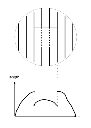
Note that condition (4) is not redundant since we could have a continuous (or even smooth) family of such that is discontinuous. In general, the function is only upper semi-continuous in . See Figure 4.1 for an example of a discontinuous sweepout of a topological annulus by curves. Here we let be a disk with a square removed and consider a sweepout of by vertical lines.This example is one dimension lower but a similar example in can be constructed easily. In fact, by Lemma 3.1, condition (4) is equivalent to saying that is a continuous family as varifolds in .
4.2. The min-max construction
Given a sweepout , we can deform the sweepout to get another sweepout by the following procedure. Let be a smooth map such that for each , there exists isotopies such that . We define a new family by . It is clear that is a sweepout in the sense of Definition 4.1. A collection of sweepouts is saturated if it is closed under these deformations of sweepouts.
Remark 4.4.
For technical reasons, we will assume that any saturated collection of sweepouts has the additional property that there exists some natural number such that for any , the set in Definition 4.1 consists of at most points.
We will apply our min-max construction to a saturated collection of sweepouts. Given any such collection , and any sweepout , we denote by the area of its maximal slice (with respect to area in ) and by the infimum of over all sweepouts in ; that is,
and
Note that we have to take “sup” in the definition of instead of “max” (as in [4]) because the maximum may not be achieved if the sweepout is not continuous.
Definition 4.5.
Given a saturated collection of sweepouts,
-
(1)
A sequence of sweepouts in is a minimizing sequence of sweepouts if
-
(2)
Let be a minimizing sequence of sweepouts. Suppose we have a sequence . We say that is a min-max sequence of surfaces if
Our goal is to show that there exists some min-max sequence converging (in the varifold sense) to a properly embedded free boundary solution (possibly with multiplicities). It is clear that the area of (counting multiplicities) is equal to . In order to produce something non-trivial, we need . We first show by an isoperimetric inequality that this can be done by choosing an initial sweepout to be the level sets of a Morse function.
Proposition 4.6.
There exists a saturated collection of sweepouts with .
Proof.
Take any Morse function on the closed 3-manifold . Define for . Then is a sweepout in the sense of Definition 4.1. Let be the saturation of , the smallest collection of sweepouts which is saturated and contains . We will show that for such a collection , we have .
Let be a smooth map such that for each , there exists isotopies such that . Define the new sweepout by . We claim that , where is a constant independent of . This would imply .
To prove our claim, let , and take , . The compact subset is a disjoint union of and , with int int. Since the function is continuous, and , Vol, there exists such that .
By the isoperimetric inequality, there exists a constant such that
Hence,
This proves our claim and thus the proposition. ∎
4.3. Convergence of min-max sequences
We now state the main convergence result which implies Theorem 1.1.
Theorem 4.7.
Let be a compact domain of a closed Riemannian 3-manifold . Given any saturated collection of sweepouts , there exists a min-max sequence of surfaces obtained from , which converges in the sense of varifolds to an integer-rectifiable varifold in with . Moreover, there exists natural numbers and smooth compact properly embedded minimal surfaces such that
where each is either closed or meets orthogonally along the free boundary .
The proof of Theorem 4.7 can be divided into three parts. The first part is a tightening argument which is similar to Birkhoff’s curve shortening process [3]. The goal is to find a good minimizing sequence of sweepouts such that almost maximal slices are almost freely stationary. This rules out the existence of almost maximal bad slices (see Figure 4 in [4]) which would not converge to a freely stationary varifold. The precise statement we will prove is the following:
Proposition 4.8.
Given a saturated collection of sweepouts, there exists a minimizing sequence of sweepouts such that
-
(1)
is a continuous sweepout for each .
-
(2)
Every min-max sequence of surfaces constructed from such a minimizing sequence has a subsequence converging weakly to a freely stationary varifold supported in .
The key new ingredient in the proposition above is a perturbation lemma which says that any sweepout can be approximated by a continuous sweepout.
Lemma 4.9.
Given any sweepout , and any , there exists a continuous sweepout such that
The proof of Lemma 4.9 is rather technical and will be presented in Appendix B. Using the perturbation lemma, one can assume, without loss of generality, that a minimizing sequence of sweepouts is continuous. Once we have continuity, the proof of Proposition 4.8 is a simple modification of the arguments in section 4 of [4]. We will give the details in section 5 of this paper.
The second part of the proof of Theorem 4.7 is to establish the existence of a min-max sequence which is outer almost minimizing on small annuli. Let and . Let be the collection of all annulus centered at with outer radius less than and inner radius greater than zero. We will prove the following existence result in section 6. A key note is that the proof requires continuity of the minimizing sequence of sweepout, which is given by Proposition 4.8.
Proposition 4.10.
Given a saturated collection , there exists a positive function and a min-max sequence of surfaces such that
-
(1)
is an outer almost minimizing sequence in any annulus An , where is any point in ;
-
(2)
In every such annulus An, is a smooth surface (possibly with boundary) when is sufficiently large;
-
(3)
The sequence converges to a freely stationary varifold in as .
The third part of the proof of Theorem 4.7 is a regularity theorem for outer almost minimizing varifolds. The idea is that the outer almost minimizing property enables us to construct replacements (see Definition 8.1) for the freely stationary varifold obtained in Proposition 4.10. It turns out that having sufficiently many replacements implies that a freely stationary varifold is regular.
Proposition 4.11.
The freely stationary varifold in Proposition 4.10 is integer rectifiable and there exists natural numbers and smooth compact properly embedded minimal surfaces such that
where each is either closed or meets orthogonally along the free boundary .
The construction of replacements involves a minimization problem among all surfaces which are outward isotopic to a fixed surface. This is a localized version of Meeks-Simon-Yau’s paper [24] with partially free boundary. In section 7, we will treat this minimization problem in detail. In section 8, we prove the regularity of freely stationary varifolds which can be replaced sufficiently many times. Combining Proposition 4.8, 4.10 and 4.11, we obtain the main convergence result (Theorem 4.7).
5. Existence of freely stationary varifolds
In this section, we show that there exists a nice minimizing sequence of sweepout such that any min-max sequence of surfaces obtained from such a minimizing sequence has a subsequence converging to a varifold in which is freely stationary. Using the perturbation lemma (Lemma 4.9), we can make the minimizing sequence continuous. This is essential in the proof of Proposition 4.8 and Proposition 4.10 in the next section.
We restate Proposition 4.8 below.
Proposition 5.1 (Proposition 4.8).
Given a saturated collection of sweepouts, there exists a minimizing sequence of sweepouts such that
-
(1)
is a continuous sweepout for each .
-
(2)
Every min-max sequence of surfaces constructed from such a minimizing sequence has a subsequence converging weakly to a freely stationary varifold supported in .
Proof.
Let be a minimizing sequence of sweepouts. By Lemma 4.9, we can assume is a continuous sweepout for each . So (1) is established.
Fix some . By Lemma 3.4, is a compact set in the weak topology. Let be a metric on whose metric topology agrees with the weak topology. By restricting ourselves to tangential vector fields in , the same argument as in section 4 of [4] gives a “tightening” map
such that
-
(a)
is continuous with respect to the weak topology on and the -norm on .
-
(b)
If , then is the identity isotopy on .
-
(c)
If , then
for some continuous strictly increasing function with .
Remark 5.2.
In step 1 of section 4 of [4], we should take when to make sure that is continuous. The rest of the argument goes through because the set of tangential vector fields is a convex subset of the set of all vector fields in . Hence, the vector field defined in step 1 of section 4 of [4] also belongs to .
Since are continuous sweepouts, for each , is a continuous family in . Therefore, is a continuous family in . By a smoothing argument (for example, one can take a convolution in the -variable), we can make it a smooth family. We use these tangential isotopies to deform the minimizing sequence to another minimizing sequence which satisfies
| (5.1) |
As is a minimizing sequence of sweepouts, we can assume that
| (5.2) |
Furthermore, the sweepouts are continuous since only tangential vector fields are used in the deformations.
Next, we claim that for every , there exist and such that whenever and , we have . To see this, we argue by contradiction. Note first that the construction of the tightening map yields a continuous and increasing function (independent of and ) such that and
| (5.3) |
Fix and choose , such that . We claim that for this choice of and , whenever and , we have . Suppose not. Then there are and such that and . Hence, from (5.1) and (5.3) we get
This contradicts (5.2). This proves our claim and the claim clearly implies (2) in Proposition 5.1. Therefore, the proof is completed. ∎
6. Existence of outer almost minimizing varifolds
In this section, we prove the existence of a min-max sequence which is outer almost minimizing on small annuli. The proof is a combinatorial argument first introduced by F. Almgren in [20]. First we recall the following definition from [4].
Definition 6.1.
Let be the set of pairs of open sets in with
Given , we say that is -outer almost minimizing in if it is -outer almost minimizing in at least one of the or .
Remark 6.2.
The significance of is that for any and , there are some with , hence .
The key lemma in this section is the following.
Lemma 6.3.
Let be a minimizing sequence as given in Proposition 5.1. Then there is a min-max sequence such that
Proof.
We will argue by contradiction. First of all, we fix a minimizing sequence satisfying Proposition 5.1 and such that
| (6.1) |
Fix . To prove the lemma, we make the following claim.
Claim 1: There exists and such that satisfies
-
(a)
is -outer almost minimizing in every .
-
(b)
.
Proof of Claim 1: We define the sets of “big slices” for each by
Note that is compact since is a continuous sweepout (by (4) in Definition 4.1). If Claim 1 is false, then for every , there exists a pair of open sets such that is not -outer almost minimizing in any one of them. So for every , there exists isotopies and such that for ,
-
(1)
for every ;
-
(2)
.
Next, we want to establish the following claim.
Claim 2: For each , there exists such that if , then for ,
-
(1’)
for every ;
-
(2’)
.
Proof of Claim 2: To see why (1’) is true, we argue by contradiction. Suppose no such exists, then there exists a sequence and such that for all ,
After passing to a subsequence, we can assume that for some . Observe that converges weakly as varifolds to as . By (2.6.2(c)) in [1] and the fact that the sweepouts are continuous, we have
This contradicts (1) above. So we can choose such that (1’) holds.
The proof of (2’) is similar. Again, if no such exists, then there exists a sequence such that for all ,
Since converges weakly to in as , thus, we have
This contradicts (2) above. Therefore, (2’) holds for some . Thus, Claim 2 is established.
For any , , let An denote the open annulus centered at with inner radius and outer radius . Let , we set as the collection of open annuli An such that . By the same argument as in Proposition 5.1 of Colding-De Lellis [4], we obtain Proposition 4.10, which we restate below.
Proposition 6.4 (Proposition 4.10).
Given a saturated collection , there exists a positive function and a min-max sequence of surfaces such that
-
(1)
is an outer almost minimizing sequence in any annulus An , where is any point in ;
-
(2)
In every such annulus An, is a smooth surface (possibly with boundary) when is sufficiently large;
-
(3)
The sequence converges to a freely stationary varifold in as .
7. A minimization problem with partially free boundary
In this section, we prove a result about minimizing area in among isotopic surfaces similar to the ones obtained by F. Almgren and L. Simon [2], W. Meeks, L. Simon and S.T. Yau [24], M. Grüter and J. Jost [14] and J. Jost [18]. Since we are restricting to the class of outward isotopies, we need to modify some of the arguments used in the papers above.
First, we define the concept of admissible open sets.
Definition 7.1.
An open set is said to be admissible if it satisfies all the following properties:
-
(i)
is smooth, i.e. is an open set with smooth boundary ;
-
(ii)
is uniformly convex in the sense that all the principal curvatures with respect to the inward normal is positive along ;
-
(iii)
the closure is diffeomorphic to the closed unit 3-ball in ;
-
(iv)
intersects transversally and is topologically an open disk;
-
(v)
the angle between and is always less than when measured in , i.e. if and are the outward unit normal of and respectively, then along .
Given a surface in , we want to minimize area (in ) among all the surfaces which are outward isotopic to and are identical to outside an admissible open set .
Definition 7.2.
Let be an admissible open set. Let be an embedded closed surface (not necessarily connected) intersecting transversally. Consider the minimization problem :
if a sequence satisfies
we say that is a minimizing sequence for the minimization problem .
Note that if two surfaces and agree in , i.e. , then the minimization problems and are equivalent since we only count area in and for any .
By a small perturbation by outward isotopies, we can always obtain a minimizing sequence so that intersects transversally for every . The key result of this section is the following theorem.
Theorem 7.3.
Let be an admissible open set, suppose is a minimizing sequence for the minimization problem defined in Definition 7.2 so that intersects transversally for each , and converge weakly to a varifold .
Then, the following holds:
-
(a)
, for some compact embedded minimal surface with smooth boundary (except possibly at ) contained in ;
-
(b)
The fixed boundary of is the same as ;
-
(c)
meets orthogonally along the free boundary of ;
-
(d)
is stable with respect to .
Remark 7.4.
It is clear that is freely stationary. The only thing we have to prove is regularity. Interior regularity follows from a localized version of [24] given in Proposition 3.3 of [7]. The regularity at the fixed boundary int is also discussed in [7]. Therefore, the only case left is the regularity at the free boundary . Hence, Theorem 7.3 says that the limit varifold is equal to a stable, smooth, properly embedded minimal surface (possibly disconnected).
The proof of Theorem 7.3 goes as follows. We first apply a version of local -reduction (see [24] and [7]) to reduce the minimization problem to the case of genus zero surfaces. Then we use a result from [18] to conclude that such minimizers are smooth.
7.1. Local -reductions
Following [7] and [24], replacing area by area in , we modify some of their definitions and propositions for our purpose. First of all, we fix such that the following lemma holds (see Lemma 4.2 of [18]).
Lemma 7.5.
There exists and , depending only on and , with the property that if is a surface in int() with and
then there exists a unique compact set such that
-
(a)
int (i.e. is bounded by modulo );
-
(b)
; and
-
(c)
, where depends only on and .
By rescaling the metric of if necessary, we can assume that in Lemma 7.5. From now on, we will assume that satisfies Lemma 7.5 with . We will generalize the notion of -reductions to allow boundary reductions as well. Suppose .
Definition 7.6.
Let and be closed (possibly disconnected) embedded surfaces in . We say that is a -reduction of and write
if the following conditions are satisfied:
-
(1)
is obtained from through a surgery in , that is,
-
(i)
is diffeomorphic to either a closed annulus or a closed half-annulus ;
-
(ii)
with each diffeomorphic to either the closed unit disk or the closed unit half-disk ;
-
(iii)
There exists a compact set embedded in , homeomorphic to the closed unit 3-ball with modulo (i.e. there exists a compact set such that ), and .
-
(i)
-
(2)
;
-
(3)
If is a connected component of containing , and is disconnected, then for each component of we have one of the following possibilities:
-
(a)
either it is a genus zero surface contained in with area ;
-
(b)
or it is not a genus zero surface.
-
(a)
We say that is -irreducible if there does not exist such that .
A immediate consequence of the above definition is the following.
Remark 7.7.
is -irreducible if and only if whenever is a closed disc or half-disk with and , then there is a closed genus 0 surface with and .
Similar to [24], we define strong -reduction as follows.
Definition 7.8.
Let and be closed (possibly disconnected) embedded surfaces in . We say that is a strong -reduction of and write
if there exists an isotopy such that
-
(1)
;
-
(2)
;
-
(3)
.
We say that is strongly -irreducible if there is no such that .
Following the same arguments in Remark 3.1 of [24], we have the following proposition.
Proposition 7.9.
Given any closed embedded surface (not necessarily connected), there exists a sequence of closed embedded surfaces (not necessarily connected) such that
where is strongly -irreducible. Furthermore, there exists a constant which depends only on genus and so that , and
Proof.
The proof is the same as the proof of Remark 3.1 in [24]. ∎
The following theorem gives our main result for strongly -irreducible surfaces . For any closed surface , we denote
where denotes the set of all surfaces which are outward isotopic to in . Let denote the union of all components such that there exists some diffeomorphic to the unit 3-ball such that and .
Theorem 7.10.
Let be an admissible open set, and be a compact subset diffeomorphic to the unit 3-ball. Assume intersects both and transversally.
Suppose is a smooth closed embedded surface (possibly disconnected) such that
-
(i)
intersects both and transversally;
-
(ii)
and is strongly -irreducible;
-
(iii)
For each component of , let be a the component in such that and . Furthermore, suppose that , where and denote the components of . Note that each is either a closed Jordan curve in or a Jordan arc with endpoints on , and each is either a disk, a half-disk or an annulus in .
Then, and there exists pairwise disjoint, connected, closed genus zero surfaces with , and . Moreover,
Furthermore, for any given , we have
for some isotopy (depending on ) which is identity on some open neighborhood of .
Although all sufficiently small disks with the same boundary are isotopic to each other, which is a crucial point in the proof of Theorem 2 in [24], not all of them are outward isotopic to each other. Therefore, we need to establish the lemma below, which says that all small disks are almost outward isotopic, modulo arbitrarily small area.
Lemma 7.11.
Let and be as in Theorem 7.10. Let be a Jordan curve in int which is either closed or having endpoints on . Let be a connected component of , which is diffeomorphic to a disk, a half-disk or an annulus. Let be a genus zero surface transversal to with , and . In addition, we assume that bounds a unique compact set modulo , i.e. int.
Then, for any , there exists an isotopy supported on a small neighborhood of such that for all and all , moreover,
In other words, we can outward isotope to approximate as close as we want.
Proof.
We divide the situation into two cases according to whether the boundary curve is closed or not.
Case 1: is a simple closed curve.
In this case, is either a closed disk or a closed annulus in . In the latter case, we will show that we can even find an isotopy supported on a neighborhood of , leaving fixed, and .
After a change of coordinate, we can assume that
-
•
is the open ball of radius in centered at origin;
-
•
is the closed unit 3-ball centered at origin;
-
•
is the upper half-ball; and
-
•
.
First, we look at the case that is a closed disk, i.e. . Let be the genus zero surface as given in the hypothesis. Note that meets at a finite number of simple closed curves , , each of which bounds a closed disk in . Since is a genus zero surface with boundary, it is clear that is homeomorphic to a 2-sphere, and thus, the compact set bounded by modulo is homeomorphic to the unit 3-ball in . Observe that if , then it is trivial that we can isotope to , holding fixed. If , we then use a tangential isotopy to deform it so that it approximates a disk disjoint from with boundary , which in turn is isotopic to . To see this, perturb each closed disk into the interior of such that the boundary of the disk stays on , call the perturbed disk, then there is a closed annulus such that and bounds a ball in . Using a tangential isotopy, we can deform such that it agrees with with an error in area as small as we want (one simply shrinks the size of the neck in ). Repeat the whole procedure for each , one can deform such that is arbitrarily close to a disk disjoint from , and we are done.
In the case that is a closed annulus, again let be the set of simple closed curves where meets . Note that all except possibly one bounds a disk in . For those which bounds a disk, we can repeat the “neck-shrinking” argument as in the previous case to eliminate them. Therefore, we can assume that together with bounds a connected genus 0 surface in . After a further change of coordinate, we can assume that , where we think of as a subset of . Next consider the outward isotopy given by the vertical translations (with some cutoff near so that it is supported in ), take a smooth function on such that along , outside a small neighborhood of disjoint from all , and elsewhere. By choosing the neighborhood of smaller and smaller, we see that the outward isotopy given by the vertical translations with cutoff would deform to approximate as close as we want. This implies our desired conclusion.
Case 2: is an arc with endpoints on .
Assume the standard setting as before after a change of coordinate, suppose for our convenience that , and . Note that intersects at a Jordan arc with the same endpoints as and a (possibly empty) finite collection of disjoint simple closed curves , . Let . By assumption, there is a compact set such that where is a genus zero surface in with . For all those , , which bounds a disk in , we can shrink down the neck as in Case 1. So we can assume without loss of generality that is connected. There are two further sub-cases: either is the outermost boundary of or it is not. In the first case, similar to the second part of Case 1 above, we can assume (up to a change of coordinate) that , where is the disk in bounded by the simple closed curve , and is the union of a graph over and cylinders contained in . Using a cutoff function as before which is zero on and the vertical translations, we can deform to approximate as close as we want. Now we are left with the case that is not the outermost boundary of . In this case, we can take where is the disk in bounded by the simple closed curve , and is the union of a graph over and cylinders contained in . Then a similar translation with cutoff will deform to approximate and we are done.
∎
Now we are ready to give a proof of Theorem 7.10.
Proof of Theorem 7.10.
The proof is almost the same as that in [24], except that we have to use Lemma 7.11 because not all small disks are outward isotopic to each other.
As in Meeks-Simon-Yau [24], we can assume that . We proceed by induction on . Denote
-
, , , and is strongly -irreducible, where .
-
the conclusion of Theorem 7.10 is true.
We will show that the statement “” is true for all . Assume it is true for . We want to show by induction that it is true for also.
Relabeling if necessary, we can assume that is innermost, i.e. for all . Since is strongly -irreducible and . By Remark 7.7, there exists a connected genus zero surface such that and . Since is innermost, . As the area of and are small, we can apply Lemma 7.5. Hence, there is a unique compact set which is bounded by modulo . Moreover, since is a genus zero surface, it is easy to see that there exists a small neighborhood of which is diffeomorphic to the unit 3-ball whose boundary is disjoint from . Because we assume that , we know that the whole neighborhood is disjoint from .
Replace by and write (which is only a Lipschitz surface), and , for each , we can select a continuous tangential isotopy such that , for , furthermore,
| (7.1) |
and
| (7.2) |
In other words, we deform to detach from . Let (smooth by suitably choosing ), for small enough, we have
-
(i)
,
-
(ii)
,
-
(iii)
.
Notice (iii) implies
-
(iii)’
.
because Lemma 7.11 implies that
| (7.3) |
Taking , following the same arguments in [24], we see that satisfies , hence holds by induction hypothesis. There must be pairwise disjoint connected genus zero surfaces contained in with , , and
| (7.4) |
Furthermore, for any ,
| (7.5) |
for some isotopy which fixes a neighborhood of . Reversing the isotopy used in (7.4) and (7.5), there are pairwise disjoint connected genus zero surfaces with , , and
| (7.6) |
Furthermore,
| (7.7) |
for some isotopy which fixes a neighborhood of .
Recall that is the compact set in bounded by , by Lemma 7.11, there exists a continuous isotopy supported on a neighborhood of fixing and
| (7.8) |
Moreover, we know that because . Consider the following two cases: (i) ; and (ii) .
In case (i), if , by taking for the unique such that , and we select for all . Also, we define a continuous outward isotopy by ; by smoothing we obtain an outward isotopy satisfying the required conditions. Here is defined by if , and if .
In case (ii), if , we define the set of pairwise disjoint connected genus 0 surfaces by setting , , and . In this case, we define a continuous isotopy by setting , where is a smooth outward isotopy such that for all and , and such that is a genus zero surface with , , and for all . Such a exists once we show the claim that in case (ii), there is a neighborhood of such that . Otherwise, we would have with and , and this would imply that since (see the statement above (7.6)), thus contradicting we are in case (ii). By smoothing we then again obtain the required outward isotopy .
In each of the above cases, we have, by (7.6), that
and hence
This proves that statement and the proof is finished by induction.
∎
We will need a replacement lemma about finite collection of genus zero surfaces with disjoint boundaries (c.f. Lemma 2 in [24]).
Lemma 7.12.
Let be a closed subset which is diffeomorphic to the unit 3-ball such that is diffeomorphic to the closed unit disk. Suppose are connected genus zero surfaces in with and . Also, assume that and that either or intersects transversally for all .
Then, there exists pairwise disjoint connected genus zero surfaces in with , and for .
Proof.
Assume that and that are already pairwise disjoint. If we can prove the required result in this case, then the general case follows by induction on .
Let be pairwise disjoint Jordan curves (either closed or have boundaries on ), not necessarily connected, such that
| (7.9) |
also, for each , divides each which contains into two genus zero surfaces (maybe disconnected) with (since are pairwise disjoint by assumption, either or is disjoint from ) and, as an inductive hypothesis, assume the lemma is true whenever (7.9) holds with replaced by on the right hand side (with still being assumed pairwise disjoint).
For each , let be the part of which is disjoint from . Hence, . Let be the corresponding part in which is disjoint from . Hence, . Let be a genus zero surface with for some such that
Let be the other genus zero surface in such that . Evidently we must have
| (7.10) |
where is such that . Let be such that (note that then one of is equal to ), and define if and . By (7.10) we have that each is an embedded genus zero surface, and clearly , , are pairwise disjoint and
| (7.11) |
By smoothing near and making a slight perturbation near , we then obtain genus 0 surfaces with , , pairwise disjoint, and (using (7.11)),
Hence, we can apply the inductive hypothesis to the collection , thus obtaining the required collection .
∎
7.2. Minimizing sequence of genus zero surfaces
In this section, we recall a result by J. Jost [18] on the regularity for minimizers of the minimization problem for genus zero surfaces with partially free boundary.
Let be an admissible open set. Let be an embedded smooth curve in which either meets at the two endpoints transversally or is disjoint from . Let be the set of all genus zero surfaces contained in with as boundary modulo , i.e. , and which meets transversally. We say that is a minimizing sequence for if
for some positive real numbers as .
Theorem 7.13 ([18]).
Using the notation above, let be a minimizing sequence for , and suppose converges to in the sense of varifolds in . Then for each point supp, there are , (both depending on ) and an embedded minimal surface in meeting orthogonally with
where is the varifold represented by with multiplicity one.
7.3. Convergence of the minimizing sequence
In this section, we prove the main regularity result (Theorem 7.3).
Proof of Theorem 7.3.
Let be a minimizing sequence for the minimization problem with converging weakly to a varifold in and intersects transversally for each . Using the same argument as in [24], we can assume that for all (see the paragraph above Theorem 7.10 for definition of ) and is strongly -irreducible for all sufficiently large k, for some fixed . Furthermore, we have
| (7.12) |
where as .
As noted before, interior regularity and regularity at fixed boundary have been discussed in [24] and [7]. So we only have to prove regularity at the free boundary.
Let supp, and be the outward unit normal at . Define be a point outside which is very close to (by choosing very small). Let be chosen small so that all the geodesic balls in are admissible open sets in the sense of Definition 7.1 for all . Note that we have to move the center of the balls from to in order for of Definition 7.1 to hold.
First of all, we want to show that is freely stationary in . Let be supported in , and be the isotopy generated by . By (7.12),
| (7.13) |
for all . Note that since , take in (7.13), we get
| (7.14) |
for all . This shows that is stable with respect to , so is freely stationary. Therefore, the monotonicity formula in [14] can be applied to .
By the coarea formula, we have
for almost every and every , where is the closed geodesic ball in of radius centered at . Taking , the monotonicity formula in [14] gives
for all sufficiently large , where depends only on and and any upper bound for (recall that is the reflection of across , see [14] for definition). Hence, we can find a sequence such that intersects transversally and such that
| (7.15) |
for all sufficiently large , provided , where for the moment is arbitrary. If is sufficiently small, we see from (7.15) that Theorem 7.10 is applicable. Hence, there are connected genus zero surfaces and for any , isotopies such that
| (7.16) |
| (7.17) |
and
where is independent of and . Since , we know that for sufficiently small, by the modified replacement lemma with free boundary (see Lemma 4.4 in [18]), there are connected genus zero surfaces contained in with
| (7.18) |
and
| (7.19) |
Combining (7.12) and (7.19), using Lemma 7.12, (7.16), (7.17) and (7.18), is a minimizing sequence among all genus zero surfaces with fixed boundary with any number of free boundaries on . By Theorem 7.13, we know that for each supp, there exist and and an embedded minimal surface meeting orthongonally with on . This finishes the proof of Theorem 7.3. ∎
8. Regularity of outer almost minimizing varifolds
In this section, we define the notion of good replacement property for freely stationary varifolds and prove that if there exists sufficiently many replacements, then the varifold must be a smooth minimal surface with free boundary. In the second half, we will describe how to construct these replacements for outer almost minimizing varifolds.
Definition 8.1.
Let be a freely stationary varifold and be an open subset. We say that is a replacement for in if and only if
-
(1)
is freely stationary;
-
(2)
on and ;
-
(3)
is (an integer multiple of) a smooth stable properly embedded (not necessarily connected) minimal surface meeting orthogonally. Here, is stable means that the second variation is nonnegative with respect to isotopies supported in and for all .
Definition 8.2.
Let be freely stationary and be an open subset. We say that has good replacement property in if and only if all the following hold:
-
(a)
There is a positive function such that for every annulus An, there is a replacement for in An1 such that (b) holds;
-
(b)
There is another positive function such that
-
(i)
has a replacement in any An, for the same and as in (a), and satisfies (c) below;
-
(ii)
has a replacement in any An for any .
-
(i)
-
(c)
There is yet another positive function such that has a replacement in any An for any .
The key result in this section is the following regularity theorem.
Theorem 8.3.
If has good replacement property in an open set , then is a smooth embedded minimal surface in int with smooth free boundary on .
The proof of interior regularity can be found in [4]. Therefore, we will only prove regularity at the free boundary. To prove Theorem 8.3, we first state a generalization of two lemmas from [4] adapted to the free boundary setting.
Lemma 8.4.
Let be an open set of and . Then, there exists some such that and there does not exist any with support contained in and freely stationary in .
Proof.
We prove the lemma in the case and . The proof for the general case is similar. Fix , let be small enough (smaller than the convexity radius of in the general case) such that . If the lemma is false, then there exists a freely stationary varifold in which is supported in . Choose to be the smallest radius such that contains the support of , then the support of either touches at a point in the interior of or on the boundary . Either case cannot happen by the maximum principle (see Lemma B.1 of [4] or Theorem 1 of [40]). Note that in the general case, we have to perturb by a projection (see [14]) the variation field to make it tangent to , but the perturbation would be small if we choose small enough, so we would still arrive at a contradiction. ∎
Given a varifold and a point , we let be the set of varifold tangents of at (see section 42 of [36]).
Lemma 8.5.
Let , and be a freely stationary integer rectifiable varifold. Assume is the subset of supp defined by
If is less than the injectivity radius inj of , then is dense in supp.
Proof.
The proof is similar to the proof of Lemma B.2 in [4]. ∎
The next proposition tells us what we can say about the freely stationary varifold if there exists one replacement.
Proposition 8.6.
Let be open and be a freely stationary varifold in . If there exists a positive function such that has a replacement in any annulus An.
Then, is integer rectifiable in . Moreover, if supp, then and any tangent cone to at is an integer multiple of a plane; if supp, then and any tangent cone to at is an integer multiple of a half-plane orthogonal to .
Proof.
Fix an supp. Since is freely stationary, the monotonicity formula (3.2) from [14] gives and a constant (depending only on and ) such that for all in some neighborhood of in , and ,
We can assume that is small enough so that Lemma 8.4 is satisfied. Choose and so that is smaller than the convexity radius of . Since , there is a replacement for in the annulus An. First of all, on An. Otherwise, since in , we have supp and there would be a such that touches from the interior, i.e. . This would contradict Lemma 8.4. Therefore, is a non-empty smooth surface in An which meets orthogonally, and so there is some An with . By the monotonicity formula, and notice that ,
For suppint, the usual monotonicity formula for stationary varifold gives a similar lower bound. Hence, is bounded uniformly from below on supp, applying the rectifiability theorem, we conclude that is rectifiable.
The interior case was handled in [4], and we know that is integer rectifiable. So it remains to prove the free boundary case in the proposition. Fix supp, and a sequence such that converges weakly to a tangent cone which is stationary with respect to all variations tangential to . By a change of coordinate, we can assume that has inward pointing normal . We will show that is an integer multiple of a half plane . Since is freely stationary, must be orthogonal to , hence contain .
First, we place by in the annulus An and set . After possibly passing to a subsequence, we can assume that weakly, where is a stationary varifold with respect to tangential variations. By the definition of replacements, we have
and
| (8.1) |
where is the ball the radius in centered at the origin. Since is a cone, using (8.1), we have
Hence, the stationarity of and the monotonicity formula imply that is also a cone. By Theorem 3.5, converges to a stable properly embedded minimal surface in An, with respect to variation fields in . This means that An is an embedded minimal cone in the classical sense and hence is supported on a half disk containing the origin. The minimal cone is not the - plane since each meets orthogonally. This forces and to coincide and be an integer multiple of the same half plane perpendicular to . ∎
We now give the proof of the main result (Theorem 8.3) in this section.
Proof of Theorem 8.3.
Again, the interior regularity is covered in section 6 of [4], so we only prove the free boundary regularity. Fix supp. Choose small such that and is less than given in Lemma 8.4 and the convexity radius of , by the good replacement property (a), we can find a replacement for in the annulus An. Let be the stable minimal surface given by in An. For any and , by the good replacement property (b)(i), we can find a replacement of in An. Let be the stable minimal surface given by in An.
First, we choose some such that intersects transversally. Such a exists because is a smooth surface in the annulus An. Next, we show that An can be glued to An smoothly. It has already been shown that they glue together smooth in the interior in [4], so it suffices to show that they also glue together smoothly along the free boundary.
Fix a point , and a sufficiently small radius so that is a half-disk orthogonal to and is a smooth arc perpendicular to . As in [4], we can assume, without loss of generality, that is the unit ball in centered at origin, , . Moreover, . Suppose is the graph of a smooth function defined on . Hence, .
The replacement consists of in . By Proposition 8.6, using the fact that satisfies (c) in Definition 8.2, consists of a family of (integer multiples) of half-planes orthogonal to (in other words, they contain the vector ). Since is regular and transversal to , each half plane coincides with the half plane in . Therefore, . Now,following the argument in [4], we obtain a function such that
Since and meets orthogonally, we have the free boundary condition for all and for all . By the reflection principle, one obtain a continuous function defined on the unit disk such that is smooth and satisfies the minimal surface equation on the punctured disk . Hence by standard interior regularity for second order uniformly elliptic PDE, is smooth across the origin.
By the maximum principle Lemma 8.4, we have shown that for any , can be extended to a surface in An such that if , then in An. Thus, is a stable minimal surface with free boundary on and . Next, we show that coincides with in . Recall that in . Fix any supp and set . Since meets orthogonally, , so we can assume int and consists of a multiple of a plane transversal to (by Lemma 8.5), then we know that as in [4]. Therefore, (2) in the definition of replacement implies that on .
It remains to show that is a removable singularity for . By Proposition 8.6, every is a multiple of a half-plane orthogonal to . Following [4], for sufficiently small, there exists natural numbers and such that
where each is a Lipschitz graph over a planar half-annulus, with the Lipschitz constants uniformly bounded independent of . Hence, we get minimal punctured half-disks with
By Allard regularity for stationary varifolds with free bounday ([14]), we see that is a removable singularity for each . Finally, by the Hopf boundary lemma for uniformly elliptic second order PDE, must be one. This completes the proof of Theorem 8.3. ∎
To finish the proof of Proposition 4.11, it remains to construct replacements for limits of outer almost minimizing min-max sequences. Let be as in Proposition 4.10 and fix an annulus An. Set
Lemma 8.7.
For each , suppose we have a minimizing sequence for the problem that converges weakly to a varifold .
Then, is a stable minimal surface in An with free boundary on . Moreover, any which is the limit of a subsequence of is a replacement for (in the sense of Definition 8.1).
Proof.
The proof of the second assertion is exactly as that in Proposition 7.5 in [4]. So we only prove the first assertion here. Without loss of generality, we assume that , and we write , and in place of , and respectively. Clearly is stationary and stable in An, by its minimizing property. Thus, we only need to prove regularity. The proof follows exactly as in [4] except that we are using Theorem 3.5, Theorem 7.3 and the following result (see Lemma 7.6 in [4]), which can be proved by a rescaling argument as in [4]:
Fact: Let , and assume that is minimizing for the problem . Then, there exists such that for sufficiently large, the following holds:
-
(Cl)
For any with , there exists another isotopy such that and
Moreover, can be chosen so that (Cl) holds for any sequence which is minimizing for the problem and with on .
∎
We end this section with a proof of Proposition 4.11.
Proof of Proposition 4.11.
We will apply Theorem 8.3. From Lemma 8.7 above, We know that in every annulus An there is a replacement for . We need to show that satisfies (a), (b) and (c) in Definition 8.2, with .
∎
9. Genus bound
In this section, we observe that a result in De Lellis-Pellandini [7] which controls the topological type of the minimal surface constructed by min-max arguments continue to hold in the case of free boundary. (We will assume that all surfaces in a sweepout is orientable as in De Lellis-Pellandini [7].) The proof is exactly the same as in De Lellis-Pellandini [7]. One only has to note that a compact smooth surface has genus if and only if the image of the map is when is orientable, or the image is if is non-orientable. The lifting lemma (Proposition 2.1 in De Lellis-Pellandini [7]) is still valid and hence the proof goes through.
Theorem 9.1.
Let be a sequence which is almost minimizing in sufficiently small annuli which intersects transversally for all and be the varifold limit of as . Write where are connected components of , counted without multiplicity and are positive. Let be the set of those which are orientable and be those which are non-orientable. Then
| (9.1) |
where denotes the genus of a smooth compact surface (possibly with boundary).
On the other hand, we note that it is impossible to get a similar bound on the connectivity (i.e. number of free boundary components) of the minimal surface. Corollary 1.3 is then a direct consequence of Theorem 1.1 and Theorem 9.1 is the following. Noting that there is no closed minimal surface in .
Corollary 9.2.
Any smooth compact domain in contains a non-trivial properly embedded minimal surface with non-empty boundary which is a free boundary solution and such that
-
(i)
either is an orientable genus zero surface, i.e. a disk with holes;
-
(ii)
or is a non-orientable genus one surface, i.e. a Möbius band with holes.
This follows from the observation that any such domain can be swept out by surfaces with genus zero. In fact, we can generalize the result to arbitrary 3-manifold. Recall that for any orientable closed 3-manifold , the Heegaard genus of is the smallest integer such that , where is an orientable surface of genus and each , , is a handlebody of genus . For manifolds with boundary, we make the following definition.
Definition 9.3.
Let be a compact 3-manifold with boundary. We define the filling genus of to be the smallest integer such that there exists a smooth embedding of into a closed orientable 3-manifold with Heegaard genus .
Since any closed 3-manifold with Heegaard genus has a non-trivial sweepout by surfaces with genus as most . The min-max construction on the saturation of such a sweepout together with the genus bound (Theorem 9.1) above give Theorem 1.2 as a corollary.
Corollary 9.4 (Theorem 1.2).
Any smooth compact orientable 3-manifold with boundary with filling genus contains a nonempty properly embedded smooth minimal surface with free boundary and the genus of is at most if it is orientable; and at most if it is not orientable.
Appendix A Proof of Lemma 3.1
We now present a proof of Lemma 3.1.
Proof.
Since is a weakly convergent sequence, is bounded. Hence is also bounded. After passing to a subsequence (we use the same index for our convenience), converges weakly to some . Since is closed in , we have . We will show that . This clearly proves our lemma, since any subsequence of has another subsequence converging weakly to .
First, we claim that , i.e. for any nonnegative continuous function on . Since is a closed subset of , there exists a decreasing sequence of continuous functions on with , on and converges pointwise to the characteristic function of . As converges weakly to in , we have for each ,
| (A.1) |
Since and are nonnegative, for each and ,
| (A.2) |
Holding fixed and taking in (A.2), by (A.1), we have
Since is supported in and on for each , we get
Now, since converges pointwise to monotonically, by the monotone convergence theorem,
This proves our claim that .
Now, we want to show that . Since we already have the inequality . It suffices to show that . It follows from the assumption that converges to as ,
Therefore, the proof of Lemma 3.1 is completed. ∎
Appendix B The perturbation lemma
We end this section by proving a technical perturbation lemma (Lemma 4.9). First, we prove a lemma which says that if we use a “small” isotopy to deform a surface, its area would not increase by too much.
Lemma B.1.
Let be a varifold in . Suppose we have a smooth vector field , and let be the outward isotopy in generated by . Then,
Here, denotes the -norm of the vector field as a smooth map .
Proof.
By the first variation formula of area in ,
Hence, if we let , then the inequality above is equivalent to
Integrating from to , we get . In other words,
Now, using this and the assumption that is an outward vector field,
where the first inequality holds because . This proves Lemma B.1. ∎
We are now ready to prove the perturbation lemma.
Lemma B.2.
Given any sweepout , and any , there exists a continuous sweepout such that
Proof.
By 2.6.2(d) of Allard [1] and Lemma 3.1 in this paper, it suffices to construct such that
| (B.1) |
for all . This would imply that is a continuous sweepout. One might hope to perturb using an outward isotopy so that it is transversal to for all . However, it is impossible, in general, to find a smooth family of outward isotopies such that all the perturbed surfaces are transversal to . On the other hand, we could find one so that all but finitely many is transversal to the boundary after perturbation, and for those finitely many exceptions, there are only finitely many points at which the perturbed meets the boundary non-transversally. This would certainly imply (B.1).
For sufficiently small (to be chosen later), the signed distance function is a smooth function on the open tubular neighborhood of . (We take to be nonnegative for points in .) Let be the inward pointing unit normal to with respect to (This is globally defined on even when is not orientable). For small enough, we have a diffeomorphism
We will need the following parametric Morse theorem: If is a one-parameter family of smooth functions on a compact (possibly with boundary) manifold with , and , are Morse functions, then there exists a smooth one-parameter family such that , , and is uniformly close to in the -topology on functions . Furthermore, is Morse at all but finitely many , at a non-Morse time, the function has only one degenerate critical point, corresponding to the birth/death transition.
The relationship between Morse functions and transversality can be seen as follows. Let be a closed surface in . Consider the function restricted on , if is a Morse function, then intersects the level sets transversally except possibly at the critical points of , which is only a finite set. In particular, we have . If is not a Morse function, we approximate it by a Morse function in norm in . Without loss of generality, we can also assume that everywhere. Let be a smooth extension of the function to (by Whitney’s extension theorem), in such a way that is very small. Then, if we consider the outward vector field
where is a smooth cutoff function on such that on , outside and . Let be the outward isotopy generated by . Then it is clear that according to the discussion above.
The perturbation can be carried out for each in the sweepout. Hence, we want to choose on which are small in norm such that, after perturbation, intersects the boundary at a set of - measure zero. The only complication is that we have to choose which depends smoothly on . This is where we need the parametric Morse theorem.
By Lemma B.1, for every and , there exists sufficiently small (for example, take ) such that whenever ,
| (B.2) |
for all with .
Fix a sweepout and as in the hypothesis, since is a continuous family of varifolds in , there exists a constant such that for all . For this and , choose so that (B.2) holds. Moreover, assume is always sufficiently small so that is a smooth function on and is a diffeomorphism.
Now, we would like to apply the parametric Morse theorem to the family of smooth functions . However, there is a little technical difficulty because are not all diffeomorphic to each other. Recall that in the definition of a sweepout, we have two finite sets, and , at which singularities occur. First of all, we argue that we can assume .
Suppose . Since is just a finite set, there exists such that . Define an outward vector field by
where is a smooth cutoff function on such that on , outside and . Let be a constant (independent of ) so that on . Hence, for sufficiently small (depending on and ), we can make . Let be the isotopy generated by , then by (B.2),
Moreover, . Therefore, replacing by if necessary, we can assume that .
As is a finite set, we can further assume that is small enough so that . By the definition of a sweepout, there exists a partition of the interval such that on each subinterval , , there exists an open neighborhood of contained in such that are all diffeomorphic for .
Now, for any (to be specified later), since Morse functions are dense in -topology, for each , we can approximate the smooth function by a Morse function , with and . Let be a smooth extension of to such that for all . Using the parametric Morse Theorem, we can construct a smooth family of smooth functions on , such that is a Morse function on except for finitely many ’s there is only one degenerate critical point. We can also assume that is uniformly small in -norm on . Putting these intervals together, we have a piecewise smooth one-parameter family of smooth functions , defined on for some neighborhood of , such that are Morse except at finitely many times. Since Morse functions form an open set in the space of all smooth functions in the -topology, and the family is Morse at each , we can smooth out the family, keeping it Morse except at finitely many times away from ’s. Assume is chosen small enough such that . In summary, we have a smooth one-parameter family of smooth non-positive functions on such that . For each , let be the outward isotopy generated by the outward vector field defined as
where is a smooth cutoff function on so that on , outside and . Let be the isotopy in generated by . Take , then . We claim that is the competitor we want.
First of all, by choosing sufficiently small, we can make for all . Hence, we have from (B.2) that
Moreover, since agrees with for all , by our construction, we have consists of at most finitely many points for all . Therefore, we have
This completes the proof of Lemma B.2. ∎
References
- [1] William K. Allard, On the first variation of a varifold, Ann. of Math. (2) 95 (1972), 417–491. MR 0307015 (46 #6136)
- [2] Frederick J. Almgren, Jr. and Leon Simon, Existence of embedded solutions of Plateau’s problem, Ann. Scuola Norm. Sup. Pisa Cl. Sci. (4) 6 (1979), no. 3, 447–495. MR 553794 (81d:49025)
- [3] George D. Birkhoff, Dynamical systems with two degrees of freedom, Trans. Amer. Math. Soc. 18 (1917), no. 2, 199–300. MR 1501070
- [4] Tobias H. Colding and Camillo De Lellis, The min-max construction of minimal surfaces, Surveys in differential geometry, Vol. VIII (Boston, MA, 2002), Surv. Differ. Geom., VIII, Int. Press, Somerville, MA, 2003, pp. 75–107. MR 2039986 (2005a:53008)
- [5] Tobias Holck Colding and William P. Minicozzi, II, A course in minimal surfaces, Graduate Studies in Mathematics, vol. 121, American Mathematical Society, Providence, RI, 2011. MR 2780140
- [6] R. Courant, The existence of minimal surfaces of given topological structure under prescribed boundary conditions, Acta Math. 72 (1940), 51–98. MR 0002478 (2,61a)
- [7] Camillo De Lellis and Filippo Pellandini, Genus bounds for minimal surfaces arising from min-max constructions, J. Reine Angew. Math. 644 (2010), 47–99. MR 2671775 (2011g:53012)
- [8] Ulrich Dierkes, Stefan Hildebrandt, and Friedrich Sauvigny, Minimal surfaces, second ed., Grundlehren der Mathematischen Wissenschaften [Fundamental Principles of Mathematical Sciences], vol. 339, Springer, Heidelberg, 2010, With assistance and contributions by A. Küster and R. Jakob. MR 2566897
- [9] Ulrich Dierkes, Stefan Hildebrandt, and Anthony J. Tromba, Regularity of minimal surfaces, second ed., Grundlehren der Mathematischen Wissenschaften [Fundamental Principles of Mathematical Sciences], vol. 340, Springer, Heidelberg, 2010, With assistance and contributions by A. Küster. MR 2760441
- [10] Ailana M. Fraser, On the free boundary variational problem for minimal disks, Comm. Pure Appl. Math. 53 (2000), no. 8, 931–971. MR 1755947 (2001g:58026)
- [11] by same author, Minimal disks and two-convex hypersurfaces, Amer. J. Math. 124 (2002), no. 3, 483–493. MR 1902886 (2003d:53104)
- [12] Karlheinz Goldhorn and Stefan Hildebrandt, Zum Randverhalten der Lösungen gewisser zweidimensionaler Variationsprobleme mit freien Randbedingungen, Math. Z. 118 (1970), 241–253. MR 0279699 (43 #5420)
- [13] M. Grüter and J. Jost, On embedded minimal disks in convex bodies, Ann. Inst. H. Poincaré Anal. Non Linéaire 3 (1986), no. 5, 345–390. MR 868522 (88f:49029)
- [14] Michael Grüter and Jürgen Jost, Allard type regularity results for varifolds with free boundaries, Ann. Scuola Norm. Sup. Pisa Cl. Sci. (4) 13 (1986), no. 1, 129–169. MR 863638 (89d:49048)
- [15] S. Hildebrandt and J. C. C. Nitsche, Minimal surfaces with free boundaries, Acta Math. 143 (1979), no. 3-4, 251–272. MR 549778 (82e:49059)
- [16] Stefan Hildebrandt, Boundary behavior of minimal surfaces, Arch. Rational Mech. Anal. 35 (1969), 47–82. MR 0248650 (40 #1901)
- [17] Willi Jäger, Behavior of minimal surfaces with free boundaries, Comm. Pure Appl. Math. 23 (1970), 803–818. MR 0266067 (42 #976)
- [18] Jürgen Jost, Existence results for embedded minimal surfaces of controlled topological type. I, Ann. Scuola Norm. Sup. Pisa Cl. Sci. (4) 13 (1986), no. 1, 15–50. MR 863634 (89m:58040)
- [19] by same author, Existence results for embedded minimal surfaces of controlled topological type. II, Ann. Scuola Norm. Sup. Pisa Cl. Sci. (4) 13 (1986), no. 3, 401–426. MR 881099 (89m:58041)
- [20] Frederick J. Almgren Jr., The theory of varifolds, Mimeographed notes, Princeton University, 1965.
- [21] Hans Lewy, On mimimal surfaces with partially free boundary, Comm. Pure Appl. Math. 4 (1951), 1–13. MR 0052711 (14,662e)
- [22] Man Chun (Martin) Li, On a free boundary problem for embedded minimal surfaces and instability theorems in manifolds with positive isotropic curvarure, Ph.D. thesis, Stanford University, 2011.
- [23] Fanghua Lin and Xiaoping Yang, Geometric measure theory—an introduction, Advanced Mathematics (Beijing/Boston), vol. 1, Science Press, Beijing, 2002. MR 2030862 (2005a:28001)
- [24] William Meeks, III, Leon Simon, and Shing Tung Yau, Embedded minimal surfaces, exotic spheres, and manifolds with positive Ricci curvature, Ann. of Math. (2) 116 (1982), no. 3, 621–659. MR 678484 (84f:53053)
- [25] William H. Meeks, III and Shing Tung Yau, Topology of three-dimensional manifolds and the embedding problems in minimal surface theory, Ann. of Math. (2) 112 (1980), no. 3, 441–484. MR 595203 (83d:53045)
- [26] William W. Meeks, III and Shing Tung Yau, The existence of embedded minimal surfaces and the problem of uniqueness, Math. Z. 179 (1982), no. 2, 151–168. MR 645492 (83j:53060)
- [27] Johannes C. C. Nitsche, The boundary behavior of minimal surfaces. Kellogg’s theorem and Branch points on the boundary, Invent. Math. 8 (1969), 313–333. MR 0259766 (41 #4399a)
- [28] by same author, Minimal surfaces with partially free boundary. Least area property and Hölder continuity for boundaries satisfying a chord-arc condition, Arch. Rational Mech. Anal. 39 (1970), 131–145. MR 0266068 (42 #977)
- [29] by same author, Stationary partitioning of convex bodies, Arch. Rational Mech. Anal. 89 (1985), no. 1, 1–19. MR 784101 (86j:53013)
- [30] Jon T. Pitts, Existence and regularity of minimal surfaces on Riemannian manifolds, Mathematical Notes, vol. 27, Princeton University Press, Princeton, N.J., 1981. MR 626027 (83e:49079)
- [31] Jon T. Pitts and J. H. Rubinstein, Existence of minimal surfaces of bounded topological type in three-manifolds, Miniconference on geometry and partial differential equations (Canberra, 1985), Proc. Centre Math. Anal. Austral. Nat. Univ., vol. 10, Austral. Nat. Univ., Canberra, 1986, pp. 163–176. MR 857665 (87j:49074)
- [32] J. Sacks and K. Uhlenbeck, The existence of minimal immersions of -spheres, Ann. of Math. (2) 113 (1981), no. 1, 1–24. MR 604040 (82f:58035)
- [33] R. Schoen, L. Simon, and S. T. Yau, Curvature estimates for minimal hypersurfaces, Acta Math. 134 (1975), no. 3-4, 275–288. MR 0423263 (54 #11243)
- [34] Richard Schoen, Estimates for stable minimal surfaces in three-dimensional manifolds, Seminar on minimal submanifolds, Ann. of Math. Stud., vol. 103, Princeton Univ. Press, Princeton, NJ, 1983, pp. 111–126. MR 795231 (86j:53094)
- [35] by same author, Minimal submanifolds in higher codimension, Mat. Contemp. 30 (2006), 169–199, XIV School on Differential Geometry (Portuguese). MR 2373510 (2009h:53137)
- [36] Leon Simon, Lectures on geometric measure theory, Proceedings of the Centre for Mathematical Analysis, Australian National University, vol. 3, Australian National University Centre for Mathematical Analysis, Canberra, 1983. MR 756417 (87a:49001)
- [37] F. Smith, On the existence of embedded minimal 2-spheres in the 3-sphere, endowed with an arbitrary Riemannian metric, Ph.D. thesis, University of Melbourne, 1982, PhD thesis, Supervisor: Leon Simon.
- [38] M. Struwe, On a free boundary problem for minimal surfaces, Invent. Math. 75 (1984), no. 3, 547–560. MR 735340 (85a:58019)
- [39] Jean E. Taylor, Boundary regularity for solutions to various capillarity and free boundary problems, Comm. Partial Differential Equations 2 (1977), no. 4, 323–357. MR 0487721 (58 #7336)
- [40] Brian White, The maximum principle for minimal varieties of arbitrary codimension, Comm. Anal. Geom. 18 (2010), no. 3, 421–432. MR 2747434
- [41] Rugang Ye, On the existence of area-minimizing surfaces with free boundary, Math. Z. 206 (1991), no. 3, 321–331. MR 1095757 (92g:58023)