Reconstruction of dark energy and expansion dynamics using Gaussian processes

Abstract

An important issue in cosmology is reconstructing the effective dark energy equation of state directly from observations. With few physically motivated models, future dark energy studies cannot only be based on constraining a dark energy parameter space, as the errors found depend strongly on the parametrisation considered. We present a new non-parametric approach to reconstructing the history of the expansion rate and dark energy using Gaussian Processes, which is a fully Bayesian approach for smoothing data. We present a pedagogical introduction to Gaussian Processes, and discuss how it can be used to robustly differentiate data in a suitable way. Using this method we show that the Dark Energy Survey - Supernova Survey (DES) can accurately recover a slowly evolving equation of state to $\sigma_{w}=\pm 0.05$ ($95\%$ CL) at $z=0$ and $\pm 0.25$ at $z=0.7$, with a minimum error of $\pm 0.025$ at the sweet-spot at $z\sim 0.16$, provided the other parameters of the model are known. Errors on the expansion history are an order of magnitude smaller, yet make no assumptions about dark energy whatsoever. A code for calculating functions and their first three derivatives using Gaussian processes has been developed and is available for download.

1 Introduction

A key problem in cosmology lies in determining whether dark energy is a cosmological constant and if not, then constraining how it evolves with cosmic time. Previously, this has been approached in a model-building way – i.e., constraining specific models of dark energy, such as quintessence models or modifications to general relativity [1]. It has been a significant problem to produce well motivated models which are not ad hoc in some way. In this sense they tend to have functional degrees of freedom – such as the quintessence potential or the ‘$f$’ in $f(R)$ theories of gravity – which have to be constrained via observations. Constraints on dark energy are currently derived after free functions in the models are parametrised in simple ways.

Alternatively, one can approach the problem in a different way and look for any deviations from a cosmological constant, irrespective of origin. The dark energy equation of state $w(z)=p(z)/\rho(z)$ is typically constrained using distance measurements as a function of redshift. The luminosity distance may be written as

$$d_{L}(z)=\frac{c(1+z)}{H_{0}\sqrt{-\Omega_{k}}}\sin{\left(\sqrt{-\Omega_{k}}\int_{0}^{z}{\mathrm{d}z^{\prime}\frac{H_{0}}{H(z^{\prime})}}\right)},$$ (1.1)

where $H(z)$ is given by the Friedmann equation,

$$H(z)^{2}=H_{0}^{2}\left\{\Omega_{m}(1+z)^{3}+\Omega_{k}(1+z)^{2}+(1-\Omega_{m}-\Omega_{k})\exp{\left[3\int_{0}^{z}\frac{1+w(z^{\prime})}{1+z^{\prime}}\mathrm{d}z^{\prime}\right]}\right\},$$ (1.2)

where $H_{0}=H(z=0)$ and $\Omega_{m,k}$ are the normalised density parameters. Without a model for dark energy it is difficult to use other observations as these require perturbations at some level, so distances are the vital observable. A common procedure here is to postulate a multiple parameter form for $w(z)$ and calculate $d_{L}(z)$. The most promising of these approaches uses a principal component analysis to construct the ‘optimal’ basis functions for $w(z)$ based on the data available [2, 3, 4]. Another uses Gaussian Processes to effectively smooth $w$ and fit it to data [5] (we discuss this work below).

An alternative method is to reconstruct $w(z)$ by directly reconstructing the luminosity-distance curve. Writing $D(z)=(H_{0}/c)(1+z)^{-1}d_{L}(z)$ as the normalised comoving distance, we have [7, 8, 9, 10]:

$$w(z)=\frac{2(1+z)(1+\Omega_{k}D^{2})D^{\prime\prime}-[(1+z)^{2}\Omega_{k}D^{\prime 2}+2(1+z)\Omega_{k}DD^{\prime}-3(1+\Omega_{k}D^{2})]D^{\prime}}{3\{(1+z)^{2}[\Omega_{k}+(1+z)\Omega_{m}]D^{\prime 2}-(1+\Omega_{k}D^{2})\}D^{\prime}}$$ (1.3)

Thus, given a distance-redshift curve $D(z)$, we can reconstruct the dark energy equation of state, assuming we know the density parameters $\Omega_{m}$ and $\Omega_{k}$. Different methods for doing this involve smoothing the data to give $D(z)$, or parametrising $D(z)$ by a function; see [6] for a comprehensive review, and [11, 12, 13, 14, 15, 16, 17, 18, 19] for alternative model independent approaches.

The direct reconstruction method is unstable because of the two derivatives of the observed function in Eq. (1.3), requiring the fitting function to accurately capture the slope and concavity of luminosity distance curve. This means that differences between the true underlying model and the fitted function due to the choice of parametrisation are amplified drastically when reconstructing $w$. Furthermore, $w$ is constructed from a quotient of functions which need to balance to obtain the correct $w$; the denominator can easily pass through zero for even small uncertainties making it especially unstable. Typical reconstruction methods usually appear to flounder even at moderate redshift for this reason. However, such problems may be considered as informing us about the real errors on $w$ without the intrinsic priors which arise when we start from a parametric form of $w$ and constrain it from there.

Indeed, even small errors in the parameters can lead to large errors in $w(z)$. This can be seen in the left panel of Fig. 1, where we have assumed that we know $D(z)$, $D^{\prime}(z)$, $D^{\prime\prime}(z)$ and $\Omega_{k}$ exactly, and have used the WMAP7 constraints on the matter density, $\Omega_{m}=0.275\pm 0.016$ [20]. A similar effect happens from uncertainties in the curvature. Even under these idealised conditions, the errors of the reconstructed $w(z)$ are large because they properly take into account the degeneracies with the density parameters [21, 22, 23, 24].

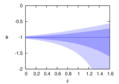
(a) $\Omega_{m}=0.275\pm 0.016$

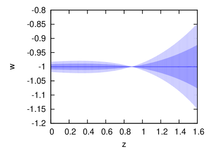
(b) $\Omega_{k}=0.00\pm 0.01$

Figure 1: Left: Dark energy reconstruction using Eq. (1.3) for $\Omega_{k}=0$, when $D(z)$ and its derivatives are exactly known ($\Lambda$CDM with $\Omega_{m}=0.275$). The uncertainty in the reconstructed $w$ (the blue shaded regions show the 68% and 95% CL) only comes from the prior on the matter density, $\Omega_{m}=0.275\pm 0.016$ (WMAP7 [20]). Right: The same plot for fixed matter density, $\Omega_{m}=0.275$, and a prior on the curvature of $\Omega_{k}=0.00\pm 0.01$.

Nevertheless, such approaches play an important role in our understanding of dark energy for several reasons. A simple one is that $w(z)$ may only be a place-holder phenomenological function supposed to encapsulate all possible alternatives to dark energy, such as modified gravity [25], and not just simple quintessence models. This means that we have to accept there could be really unexpected behaviour. An important example of this happens if $\rho_{\mathrm{eff}}$ passes through zero at some $z$ while $p_{\mathrm{eff}}$ remains non-zero, then $w(z)$ has a pole at $z$. To evaluate the integral appearing in $H(z)$ requires integration around the pole, and the residue of the integral taken into account (assuming it is defined). No method which starts from a set of basis functions for $w(z)$ can recover this behaviour if it is not known a priori.

Consider the explanation for dark energy suggested by causal set theory [26] wherein we should expect the value of $\Lambda$ to stochastically fluctuate around the Hubble scale. In that case, $w$ would be discontinuous and varying widely over short redshift scales, but this can never be represented by choosing simple functions in $w$-space.

Because of these reasons, methods which start from $w$ and work towards $D(z)$ can underestimate the errors in our understanding of dark energy. The errors which appear to condemn reconstruction methods which start from $D(z)$ and work towards $w$ are actually much more representative of our genuine errors in this regard. It is for this reason that it is important to pursue reconstruction methods, even though they are very challenging.

In this work, we use Gaussian processes for the reconstruction of $D(z)$ and its derivatives. Then equation (1.3) is used to determine $w(z)$. Gaussian processes describe a distribution over functions and are thus a generalisation of Gaussian distributions to function space. The analysis is fully Bayesian; we start with a prior for the function distribution and combine it with the likelihood of observing the data, given that distribution. This leads to a posterior function distribution.

Gaussian processes in combination with MCMC methods have previously been used to reconstruct $w(z)$ by Holsclaw et al. [5, 27]. While their method uses integration over $w(z)$ to obtain the distance, we reconstruct $D(z)$ and its derivatives in order to determine $w(z)$. Gaussian processes typically have an implicit prior favoring smooth functions. This is closely related to the preference of simpler models in Bayesian model selection. So in our approach we have a smoothness prior on our distance data, whereas, by applying the GP to $w(z)$ directly the smoothness prior is rather different in [5, 27]. As we shall see we find different results at high redshift. A comparison of the two methods will be given in Section 4.

The outline of the paper is as follows: We start with an introduction to Gaussian processes, including a performance test for the reconstruction of a function and its derivatives. In Section 3, Gaussian processes are used to reconstruct $H(z)$, $q(z)$ and $w(z)$ for a mock SN data set and for the Union2.1 data set [28]. The results are discussed in Section 4.

2 Gaussian Processes

In this section, we summarise the Gaussian process algorithm, which can perform a reconstruction of a function from data without assuming a parametrisation of the function. We mainly follow the book by Rasmussen and Williams [29]. Other useful references may be found in [30, 31] and on the Gaussian Process webpage [32]. We have developed a code for Gaussian processes called GaPP (Gaussian Processes in Python) which is available for download. It can be used to reconstruct a function and its derivatives, from a given data set.

Given a data set $\mathcal{D}$ of $n$ observations:

$$\mathcal{D}=\{(x_{i},y_{i})|i=1,\dots,n\}$$ (2.1)

we would like to reconstruct a function $f(x)$ that describes the data. We write the set of training inputs, i.e. the locations $\{x_{i}\}_{i=1}^{n}$ of the observations, as $\bm{X}$. The locations, at which we want to reconstruct the function, are denoted as $\bm{X}^{*}$.

2.1 Reconstructing a function

A Gaussian process is the generalisation of a Gaussian distribution. While the latter is the distribution of a random variable, the Gaussian process describes a distribution over functions. Consider a function $f$ formed from a Gaussian process. The value of $f$ when evaluated at a point $x$ is a Gaussian random variable with mean $\mu(x)$ and variance $\text{Var}(x)$. The function value at $x$ is not independent of the function value at some other point $\tilde{x}$ (especially when $x$ and $\tilde{x}$ are close to each other), but is related by a covariance function $\text{cov}\left(f(x),f(\tilde{x})\right)=k(x,\tilde{x})$. Thus, the distribution of functions can be described by the following quantities:

$$\mu(x) = \mathbb{E}[f(x)]\,,$$ (2.2)

$$k(x,\tilde{x}) = \mathbb{E}[(f(x)-\mu(x))(f(\tilde{x})-\mu(\tilde{x}))]\,,$$ (2.3)

$$\text{Var}(x) = k(x,x)\,.$$ (2.4)

The Gaussian process is written as

$$f(x)\sim\mathcal{GP}\left(\mu(x),k(x,\tilde{x})\right)\;.$$ (2.5)

There is a wide range of possible covariance functions. While one will often chose covariance functions that only depend on the distance between the input points $|x-\tilde{x}|$, this is not a necessary requirement. Throughout this work, we use the squared exponential covariance function:

$$k(x,\tilde{x})=\sigma_{f}^{2}\exp\left(-\frac{(x-\tilde{x})^{2}}{2\ell^{2}}\right)\;.$$ (2.6)

This function has the advantage that it is infinitely differentiable, which is useful for reconstructing the derivative of a function. The squared exponential covariance function depends on the two ‘hyperparameters’ $\sigma_{f}$ and $\ell$. In contrast to actual parameters, the hyperparameters do not specify the form of a function. Instead they characterize the “bumpiness” of the function. The characteristic length scale $\ell$ can be thought of as the distance one has to travel in $x$-direction to get a significant change in $f(x)$, whereas the signal variance $\sigma_{f}$ denotes the typical change in the $y$-direction.

For a set of input points $\bm{X}=\{x_{i}\}$, the covariance matrix $K(\bm{X},\bm{X})$ is given by $[K(\bm{X},\bm{X})]_{ij}=k(x_{i},x_{j})$. Even without any observations, one can use the covariance matrix to generate a random function $f(x)$ from the Gaussian process, i.e. one generates a Gaussian vector ${\bm{f}^{*}}$ of function values at $\bm{X}^{*}$ with $f^{*}_{i}=f(x^{*}_{i})$:

$${\bm{f}^{*}}\sim\mathcal{N}\left(\text{\boldmath$\mu^{*}$},K(\bm{X}^{*},\bm{X}^{*})\right)\;,$$ (2.7)

where $\mu^{*}$ is the a priori assumed mean of ${\bm{f}^{*}}$. The notation $\mathcal{N}$ means the Gaussian process $\mathcal{GP}$ is evaluated at specific points $x^{*}$, where $f(x^{*})$ is a random value drawn from a normal distribution. As the function is not restricted by any observations, it is quite arbitrary. Its values at different locations $x^{*}_{i}$ are however correlated by the covariance function. This can be considered as a prior on the choice of output functions; only when we add in data at other points $x_{i}$ does the output become constrained further.

Observational data $(x_{i},y_{i})$ can also be described by a Gaussian process, assuming the errors are Gaussian. The actual observations are assumed to be scattered around the underlying function, i.e. $y_{i}=f(x_{i})+\epsilon_{i}$, where Gaussian noise $\epsilon_{i}$ with variance $\sigma_{i}^{2}$ is assumed. This variance has to be added to the covariance matrix:

$${\bm{y}}\sim\mathcal{N}\left(\text{\boldmath$\mu$},K(\bm{X},\bm{X})+C\right)\,,$$ (2.8)

where $C$ is the covariance matrix of the data. For uncorrelated data we have simply $C=\text{diag}(\sigma_{i}^{2})$. The two Gaussian processes for ${\bm{f}^{*}}$ and ${\bm{y}}$ can be combined in the joint distribution:

$$\begin{bmatrix}{\bm{y}}\\ {\bm{f}^{*}}\end{bmatrix}\sim\mathcal{N}\left(\begin{bmatrix}\text{\boldmath$\mu$}\\ \text{\boldmath$\mu^{*}$}\end{bmatrix},\begin{bmatrix}K(\bm{X},\bm{X})+C&K(\bm{X},\bm{X}^{*})\\ K(\bm{X}^{*},\bm{X})&K(\bm{X}^{*},\bm{X}^{*})\end{bmatrix}\right)$$ (2.9)

While ${\bm{y}}$ is known from observations, we want to reconstruct ${\bm{f}^{*}}$. This can be done with the conditional distribution (see the Appendix)

$${\bm{f}^{*}}|\bm{X}^{*},\bm{X},\bm{y}\sim\mathcal{N}\left(\overline{\bm{f}^{*}},\text{cov}({\bm{f}^{*}})\right)\;,$$ (2.10)

where

$$\overline{\bm{f}^{*}}=\text{\boldmath$\mu^{*}$}+K(\bm{X}^{*},\bm{X})\left[K(\bm{X},\bm{X})+C\right]^{-1}({\bm{y}}-\text{\boldmath$\mu$})$$ (2.11)

and

$$\text{cov}({\bm{f}^{*}})=K(\bm{X}^{*},\bm{X}^{*})-K(\bm{X}^{*},\bm{X})\left[K(\bm{X},\bm{X})+C\right]^{-1}K(\bm{X},\bm{X}^{*})$$ (2.12)

are the mean and covariance of ${\bm{f}^{*}}$, respectively. The variance of ${\bm{f}^{*}}$ is simply the diagonal of $\text{cov}({\bm{f}^{*}})$. Eq. (2.10) is the posterior distribution of the function given the data and the prior Eq. (2.7).

In order to be able to use the above equations for reconstructing a function, we still need to know the hyperparameters $\sigma_{f}$ and $\ell$. They can be trained by maximizing the marginal likelihood, which is the marginalization over function values ${\bm{f}}$ at locations $\bm{X}$:

$$p({\bm{y}}|\bm{X},\sigma_{f},\ell)=\int p({\bm{y}}|{\bm{f}},\bm{X})p({\bm{f}}|\bm{X},\sigma_{f},\ell)d{\bm{f}}\;.$$ (2.13)

Note that the marginal likelihood only depends on the locations $\bm{X}$ of the observations, but not on the points $\bm{X}^{*}$, where we want to reconstruct the function.

With a Gaussian prior ${\bm{f}}|\bm{X},\sigma_{f},\ell\sim\mathcal{N}(\text{\boldmath$\mu$},K(\bm{X},\bm{X}))$ and with ${\bm{y}}|{\bm{f}}\sim\mathcal{N}({\bm{f}},C)$, the integration of (2.13) yields the log marginal likelihood

$$\ln\mathcal{L} = \ln p({\bm{y}}|\bm{X},\sigma_{f},\ell)$$ (2.14)

$$= -\frac{1}{2}({\bm{y}}-\text{\boldmath$\mu$})^{T}\left[K(\bm{X},\bm{X})+C\right]^{-1}({\bm{y}}-\text{\boldmath$\mu$})-\frac{1}{2}\ln\left|K(\bm{X},\bm{X})+C\right|-\frac{n}{2}\ln 2\pi\;.$$

The hyperparameters $\sigma_{f}$ and $\ell$ can now be optimized by maximizing equation (2.14).

In a completely Bayesian analysis, one should marginalise over the hyperparameters instead of optimising them. This can be done with MCMC methods. However in most cases, the log marginal likelihood is sharply peaked. Thus, the optimisation is a very good approximation of the marginalisation.

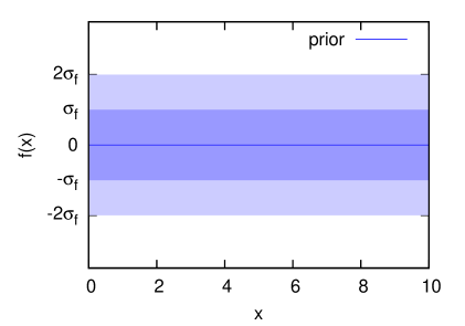
(a) prior

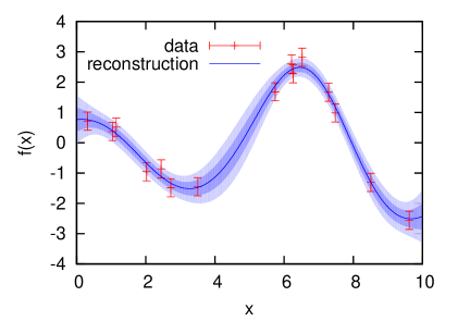
(b) posterior

Figure 2: Left: Prior of the Gaussian process as given by Eq. (2.7). Note that the hyperparameters have not been trained yet. Right: Posterior of the Gaussian process as given by Eq. (2.10).

Figure 2 shows an example for the prior and the posterior of a Gaussian process, where we have assumed a zero a priori mean function $\mu(x)=0$. For the prior, the hyperparameters have not been trained yet. Thus, the scale of the $y$-axis is not fixed and all functions are still possible. Adding data constrains the function space, which can be seen in the plot for the posterior.

How to GP

The key steps involved in constructing the $\mathcal{GP}$ are:

• Choose your data set.

• Choose a covariance function.

• Choose points $x^{*}_{i}$ where we want the function $f^{*}_{i}$ to be estimated.

• Decide a prior mean function $\mu(x)$. $\mu=\,$const. is a safe choice.

• Train the hyperparameters:

  • Carefully choose initial values for the hyperparameters. It is recommended to try different initial values because sometimes the optimisation of the hyperparameters can get stuck in a local maximum.

  • Maximise the likelihood function, Eq. (2.14), for the hyperparameters.

• Calculate $\overline{\bm{f}^{*}}$ from Eq. (2.11). This gives the expected value function.

• Calculate the diagonal elements of $\text{cov}(\bm{f}^{*})$, Eq. (2.12). This gives the variance of $\bm{f}^{*}$.

2.2 Reconstructing the derivative of a function

This method can also be used to reconstruct derivatives of $f(x)$ as the derivative of a Gaussian process is again a Gaussian process. While the covariance between the observational points stays the same, one also needs a covariance between the function and its derivative and one between the derivatives for the reconstruction. These covariances can be obtained by differentiating the original covariance function:

$$\text{cov}\left(f_{i},\frac{\partial f_{j}}{\partial x_{j}}\right)=\frac{\partial k(x_{i},x_{j})}{\partial x_{j}}$$ (2.15)

and

$$\text{cov}\left(\frac{\partial f_{i}}{\partial x_{i}},\frac{\partial f_{j}}{\partial x_{j}}\right)=\frac{\partial^{2}k(x_{i},x_{j})}{\partial x_{i}\partial x_{j}}$$ (2.16)

Covariances for higher derivatives of $f$ are calculated analogously.

Given the Gaussian process for $f(x)$, the Gaussian processes for the first and second derivative are consequently given by:

$$f(x) \sim \mathcal{GP}\left(\mu(x),k(x,\tilde{x})\right)$$ (2.17)

$$f^{\prime}(x) \sim \mathcal{GP}\left(\mu^{\prime}(x),\frac{\partial^{2}k(x,\tilde{x})}{\partial x\,\partial\tilde{x}}\right)$$ (2.18)

$$f^{\prime\prime}(x) \sim \mathcal{GP}\left(\mu^{\prime\prime}(x),\frac{\partial^{4}k(x,\tilde{x})}{\partial x^{2}\,\partial\tilde{x}^{2}}\right)$$ (2.19)

In the following, we only show the procedure for reconstructing the first derivative of $f$. Reconstructions of higher derivatives are done analogously. The joint distribution of ${\bm{y}}$ and ${\bm{f}^{*}}^{\prime}$ is

$$\begin{bmatrix}{\bm{y}}\\ {\bm{f}^{*}}^{\prime}\end{bmatrix}\sim\mathcal{N}\left(\begin{bmatrix}\text{\boldmath$\mu$}\\ \text{\boldmath$\mu^{*}$}^{\prime}\end{bmatrix},\begin{bmatrix}K(\bm{X},\bm{X})+C&K^{\prime}(\bm{X},\bm{X}^{*})\\ K^{\prime}(\bm{X}^{*},\bm{X})&K^{\prime\prime}(\bm{X}^{*},\bm{X}^{*})\end{bmatrix}\right)\;,$$ (2.20)

where

$$[K^{\prime}(\bm{X},\bm{X}^{*})]_{ij}=\frac{\partial k(x_{i},x^{*}_{j})}{\partial x^{*}_{j}}$$ (2.21)

and

$$[K^{\prime\prime}(\bm{X}^{*},\bm{X}^{*})]_{ij}=\frac{\partial^{2}k(x^{*}_{i},x^{*}_{j})}{\partial x^{*}_{i}\,\partial x^{*}_{j}}\;.$$ (2.22)

$K^{\prime}(\bm{X}^{*},\bm{X})$ is the transpose of $K^{\prime}(\bm{X},\bm{X}^{*})$.

Then the conditional distribution is given by:

$${\bm{f}^{*}}^{\prime}|\bm{X}^{*},\bm{X},y\sim\mathcal{N}\left(\overline{{\bm{f}^{*}}^{\prime}},\text{cov}({\bm{f}^{*}}^{\prime})\right)\;,$$ (2.23)

where

$$\overline{{\bm{f}^{*}}^{\prime}}=\text{\boldmath$\mu^{*}$}^{\prime}+K^{\prime}(\bm{X}^{*},\bm{X})\left[K(\bm{X},\bm{X})+C\right]^{-1}({\bm{y}}-\text{\boldmath$\mu$})$$ (2.24)

$$\text{cov}({\bm{f}^{*}}^{\prime})=K^{\prime\prime}(\bm{X}^{*},\bm{X}^{*})-K^{\prime}(\bm{X}^{*},\bm{X})\left[K(\bm{X},\bm{X})+C\right]^{-1}K^{\prime}(\bm{X},\bm{X}^{*})$$ (2.25)

The hyperparameters are trained in the same way as for the reconstruction of $f(x)$ since the marginal likelihood (2.14) that has to be maximized only depends on the observations, but not on the function we want to reconstruct.

2.3 Combining $f(x)$ and its derivatives

Often we are not only interested in reconstructing $f(x)$ and its derivatives, but also in calculating functions $g(f(x),f^{\prime}(x),\dots)$, which depend on the function derived by the Gaussian process. Then we need to know the covariances between $f^{*}=f(x^{*})$, $f^{*}{}^{\prime}=f^{\prime}(x^{*})$ $\dots$ at each point $x^{*}$ where $g$ is to be reconstructed. These covariances are given by:

$$\text{cov}(f^{*(i)},f^{*(j)})=k^{(i,j)}(x^{*},x^{*})-K^{(i)}(x^{*},\bm{X})\left[K(\bm{X},\bm{X})+C\right]^{-1}K^{(j)}(\bm{X},x^{*})\,,$$

where $f^{*(i)}$ is the $i$th derivative of $f^{*}$. $k^{(i,j)}(x^{*},x^{*})$ means that $k(x^{*},x^{*})$ is derived $i$ times with respect to the first argument and $j$ times with respect to the second argument.

At each point $x^{*}$, $g^{*}=g(f^{*},f^{*}{}^{\prime}\dots)$ is then determined by Monte Carlo sampling, where in each step $f^{*}$, $f^{*}{}^{\prime}$ $\dots$ are drawn from a multivariate normal distribution:

$$\begin{bmatrix}{f^{*}}\\ {f^{*}{}^{\prime}}\\ \vdots\end{bmatrix}\sim\mathcal{N}\left(\begin{bmatrix}\bar{f^{*}}\\ \bar{f^{*}{}^{\prime}}\\ \vdots\end{bmatrix},\begin{bmatrix}\text{var}(f^{*})&\text{cov}(f^{*},f^{*}{}^{\prime})&\cdots\\ \text{cov}(f^{*},f^{*}{}^{\prime})&\text{var}(f^{*}{}^{\prime})&\cdots\\ \vdots&\vdots&\ddots\end{bmatrix}\right)\,.$$ (2.26)

Instead of Monte Carlo sampling, one might use propagation of errors to determine the confidence levels of $g(f(x),f^{\prime}(x),\dots)$. This is however a first order approximation and is thus only recommended if the errors are small, which is usually not the case when higher derivatives are involved.

2.4 Performance of the reconstruction

Theoretically, the true function value at a point $x^{*}$ lies between the 1-$\sigma$ limits of the reconstructed function (i.e. between $f(x^{*})-\sqrt{\text{Var}(x^{*})}$ and $f(x^{*})+\sqrt{\text{Var}(x^{*})}$) with a probability of 68%. Thus, when reconstructing a function over an interval in $x$ direction, one would expect the true function to lie between the 1-$\sigma$ limits within 68% of that interval range. Note that this is only the expectation value. For one specific reconstruction this percentage might be higher or lower.

In this section, we analyse how this percentage depends on the function that we want to reconstruct. It is a reasonable assumption that – given the same amount of data – functions that change very rapidly are more difficult to reconstruct than smooth functions. In order to test this assumption we consider different superpositions of sin-waves:

$$f^{(N)}(x)=\sum_{i}^{N}\frac{a_{i}}{b_{i}^{2}}\sin(b_{i}x)\;,$$ (2.27)

where $N$ is the number of superpositions. The $a_{i}$ are random numbers between 0.5 and 1, and with random sign. The $b_{i}$ are approximately equal to $i$. (We have not used the exact equality, because that would have made it easier for the Gaussian Process to recognise the frequencies.) We have chosen functions in which the high frequency terms are suppressed compared to the low frequency ones as this provides the most difficult test for a data smoothing techniques ability to reconstruct derivatives, and is closest to our problem at hand. While in the second derivative of $f^{(N)}(x)$ the amplitudes of the different frequencies have the same order of magnitude, higher frequencies are suppressed in the function itself and (to a lesser degree) in the first derivative. This is shown in Fig. 3 for $N=10$. The function is much smoother than its derivatives.

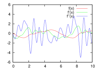
Figure 3: $f^{(10)}(x)$ from equation (2.27) and its first and second derivative.

We have then repeatedly created mock data scattered around $f^{(N)}(x)$, $N=1-10$, with varying noise ($\sigma=0.05,0.1,0.3,0.5$) and varying number of data ($n=20,50,70,100,200$). From each mock data set, we have reconstructed the function and its derivatives using Gaussian Processes. We then determined the fractions of the range interval, where the true functions $f^{(N)}(x)$, $f^{(N)}{}^{\prime}(x)$ and $f^{(N)}{}^{\prime\prime}(x)$ lie between the 1$\sigma$ and 2$\sigma$ limits of their respective reconstructions. The result is shown in Fig. 4. Each point corresponds to the average over 200 realizations of the mock data set.

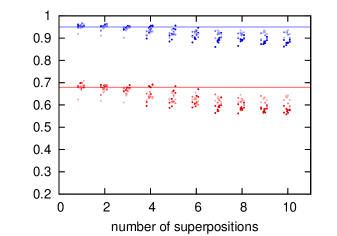
(a) $f^{(N)}(x)$

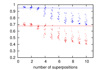
(b) $f^{(N)}{}^{\prime}(x)$

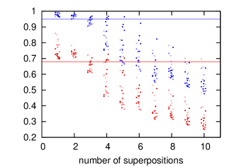
(c) $f^{(N)}{}^{\prime\prime}(x)$

(d)

Figure 4: The function $f^{(N)}(x)$ from Eq. (2.27) and its first and second derivatives are reconstructed using a GP, for different numbers of superpositions of sine waves $N$. We show the fractions of the range interval where the true function (top left) and its derivatives (first, top right; second, bottom left) a lie between the expected 1- and 2-$\sigma$ limits (1-$\sigma$: red points, 2-$\sigma$: blue points; the red and blue lines are the respective expectation values). Each point is the result of averaging over 200 mock data sets. Data sets with a smaller number of data are slightly shifted to the left, those with larger numbers to the right.

The reconstruction of $f^{(N)}(x)$ gives results that are quite close to the expected values. However, when high frequencies are involved, the errors of the reconstructed function are slightly underestimated, leading to a smaller fraction of the true function lying between the reconstructed 1$\sigma$ and 2$\sigma$ limits. When the Gaussian Process fails to recognise high frequencies, this only has a small effect on the reconstruction of $f^{(N)}(x)$, as the high frequencies are suppressed. However, this effect becomes large for the derivatives $f^{(N)}{}^{\prime}(x)$ and $f^{(N)}{}^{\prime\prime}(x)$.

We could be faced with this problem when reconstructing $w(z)$. If $w(z)$ had high frequency contributions they would be suppressed in the luminosity distance because one has to integrate twice to obtain $d_{L}(z)$ from $w(z)$ using equations (1.1) and (1.2).

On the other hand, the errors in $f^{(N)}{}^{\prime}(x)$ and $f^{(N)}{}^{\prime\prime}(x)$ are overestimated in the absence of high frequency terms. Thus, the errors of the reconstruction reflect our lack of knowledge about the frequencies that contribute to the differentiated function. Oscillations that are present in the derivatives are in general smoothed by integration and therefore hard to detect in the function. The Gaussian process accounts for that ignorance by choosing a balance between the cases where high frequencies are present or absent.

This balance is achieved by a weighted average over function space, where more weight is on smoother functions. These represent simpler models, which are preferred in Bayesian analysis. This can be seen when we perform the average over the vector of function values $\bm{f}^{*}$ (see Eq. (A)). These function values are not independent from each other, but are linked by covariances. When we consider two points $x_{1}^{*}$ and $x_{2}^{*}$, then similar values of $f(x_{1}^{*})$ and $f(x_{2}^{*})$ are preferred, unless observational evidence indicates a difference in their values. Consequently, the smoothest functions that are consistent with the observations are preferred to functions with higher frequencies.

3 Reconstruction of $H(z)$, $q(z)$ and $w(z)$

There are many functions of the distance data which provide information about dark energy dynamics. We use, in addition to the distance and its first and second derivatives, the Hubble rate, $H(z)$, the deceleration parameter $q(z)$, and $w(z)$. We assume $\Omega_{k}=0$ here so $H(z)$ provides information about the dark energy density without the degeneracy with $\Omega_{m}$. Similarly, $q(z)$ provides information about deviations from $\Lambda$CDM without this degeneracy too.

3.1 Mock data

We shall now use the GP method to smooth over a mock SNIa catalogue, and reconstruct the functions $H(z)$, $q(z)$ and $w(z)$ for a given dark energy model. As we are using the dimensionless distance $D(z)$, the analysis of the mock data set does not depend on the present Hubble rate $H_{0}$.

The Dark Energy Survey (DES) - Supernova Survey [33] is expected to obtain high quality light-curves for about 4000 SNe Ia up to redshift $z=1.2$ in the next five years. We use the anticipated redshift histogram given in [33], to create mock data sets for different dark energy models: $\Lambda$CDM and a model with slowly evolving $w(z)$. The aim of this section is to determine if the Gaussian process can recover the correct behaviours of the respective models.

In the following, we will assume a flat universe, $\Omega_{k}=0$. Then the Hubble rate is given by

$$H(z)=\frac{H_{0}}{D^{\prime}(z)}$$ (3.1)

and the deceleration parameter by

$$q(z)=-\frac{D^{\prime\prime}(z)}{D^{\prime}(z)}(1+z)-1\;.$$ (3.2)

For the reconstruction of $w(z)$, we set $\Omega_{m}=0.3$, which is the same matter density used to create the mock data sets.

3.1.1 $\Lambda$CDM

We start with a $\Lambda$CDM model with $\Omega_{m}=0.3$. We created a mock data set according to anticipated results from DES and used Gaussian processes (with $\mu(z)=0$) to reconstruct the distance $D(z)$ and its derivatives. The result is shown in Fig. 5. The blue line shows the mean of the reconstruction and the shaded areas its 68% and 95% CL. $D(z)$ is reconstructed with very high precision within the redshift range of the data. At higher redshifts the errors on the reconstruction increase, which is an expected behaviour. For the first derivative, the point where the errors start to increase significantly is shifted to lower redshifts.

The distance-redshift relation $D(z)$ of the $\Lambda$CDM model (red line) and its derivatives are reconstructed nicely by the Gaussian process.

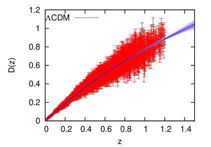
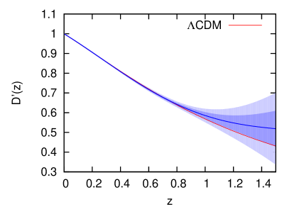
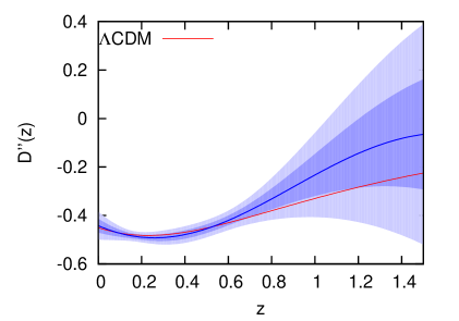
Figure 5: Reconstruction of $D(z)$, $D^{\prime}(z)$ and $D^{\prime\prime}(z)$ obtained from a mock data set following DES specifications and assuming a $\Lambda$CDM model with $\Omega_{m}=0.3$ (red line). The shaded blue regions are the 68% and 95% CL of the reconstruction.

As the Hubble rate $H(z)/H_{0}$ is simply the inverse of $D^{\prime}(z)$ (when assuming $\Omega_{k}=0$), its reconstruction is also very precise. This is shown in Fig. 6.

The formula for the reconstruction of $q(z)$ is slightly more complex and contains the first and second derivatives of the distance [see Eq. (3.2)]. This leads to larger errors at high redshifts. At low redshifts however, we get tight error bars – see Fig. 6.

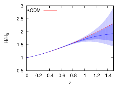
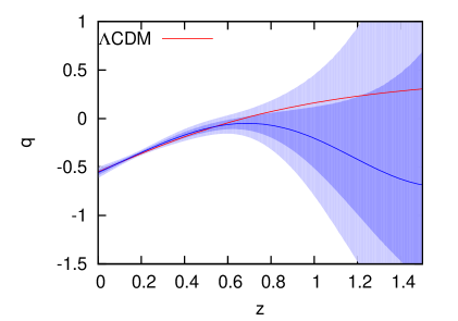
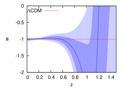
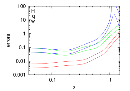
Figure 6: Reconstruction of $H(z)$ (top left), $q(z)$ (top right) and $w(z)$ (bottom left) obtained from a mock data set following DES specifications and assuming a $\Lambda$CDM model with $\Omega_{m}=0.3$ (red line). The shaded blue regions are the 68% and 95% CL of the reconstruction. The errors on $w(z)$ correctly blow up past $z\sim 1$ where there is limited data, and the effect of $w$ on distances is suppressed. The bottom right plot shows the widths of the 68% and 95% CL regions.

The reconstruction of the equation of state $w(z)$ requires a more complicated formula (1.3). Especially when the true value of the denominator is close to zero, small errors in the distance can lead to large errors in $w(z)$. In fact it can be seen in Fig. 6 that the reconstruction errors explode at redshifts $z\gtrsim 0.7$. While the true model lies within the reconstructed 95% CL, a large variety of evolving dark energy models would also be consistent with this reconstruction.

3.1.2 Evolving $w$

Next, we test a model with a slowly evolving equation of state:

$$w(z)=\frac{1}{2}\left(-1+\tanh\left[3\left(z-\frac{1}{2}\right)\right]\right)\;.$$ (3.3)

The results are shown in Fig. 7. The Gaussian process capture the model (black line) correctly for $H(z)$, $q(z)$ and $w(z)$. Also shown is a $\Lambda$CDM model, which is not consistent with the reconstruction. Thus, the Gaussian process can correctly distinguish between these two models, assuming that we know the matter density accurately enough.

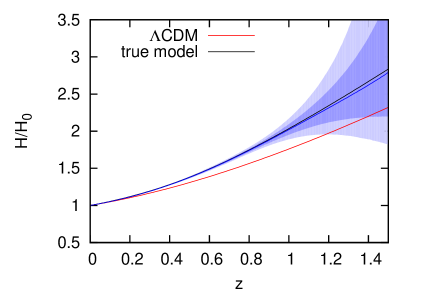
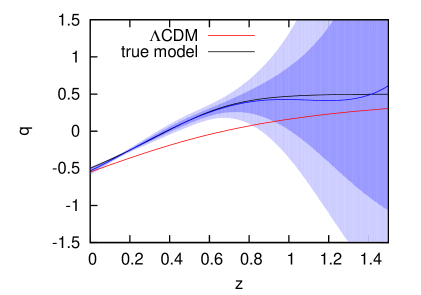
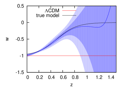
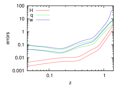
Figure 7: Reconstruction of $H(z)$, $q(z)$ and $w(z)$ obtained from a mock data set following DES specifications and assuming a model with $w(z)=0.5(-1+\tanh[3(z-0.5)])$ and $\Omega_{m}=0.3$ (red line). The shaded blue regions are the 68% and 95% CL of the reconstruction. The bottom right plot shows the widths of the 68% and 95% CL regions.

3.2 Union2.1 SNIa data

In this section, we apply the Gaussian process to real SN Ia data We use the Union2.1 data set [28], which contains 580 SNe Ia. We transformed the distance modulus $m-M$ given in the data set to $D$ using

$$m-M+5\log\left(\frac{H_{0}}{c}\right)-25=5\log((1+z)D)$$ (3.4)

with $H_{0}=70$km/(s Mpc). Note that the values of $D$ do not depend on $H_{0}$ itself, but on a combination of $H_{0}$ and the absolute magnitude $M$, which can be written as $\mathcal{M}=M-5\log\left({H_{0}}/{c}\right)+25$. To account for various systematics in the data set – such as the calibration of the absolute magnitude – we use the full covariance matrix for the data. The Gaussian process analysis implicitly assumes that the errors in $D$ follow a Gaussian distribution. However, (relatively) small deviations from Gaussianity do not affect the result of the Gaussian process significantly.

The reconstruction of the distance is shown in Fig. 8. As expected the errors of the reconstruction are larger than determined in 3.1 for the upcoming DES survey due the smaller number of SNe Ia and larger measurement errors. The reconstructions for the distance, as well as for $H(z)$, $q(z)$ and $w(z)$ (cf. Fig. 9) are consistent with $\Lambda$CDM. For the reconstruction of $w(z)$ we have assumed $\Omega_{m}=0.270\pm 0.015$, which is the constraint on the matter density for a flat universe with time dependent equation of state given in [28].

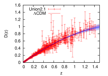
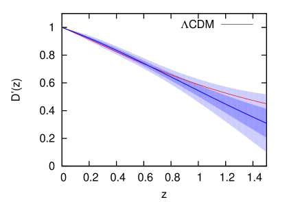
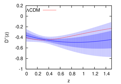
Figure 8: Reconstruction of $D(z)$, $D^{\prime}(z)$ and $D^{\prime\prime}(z)$ obtained from the Union2.1 SN data set. The shaded blue regions are the 68% and 95% CL of the reconstruction. Also shown is a $\Lambda$CDM model with $\Omega_{m}=0.27$.

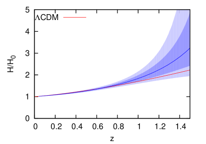
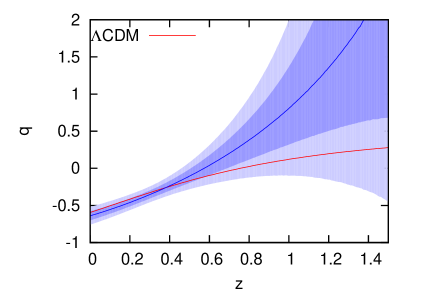
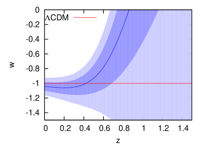
Figure 9: Reconstruction of $H(z)$, $q(z)$ and $w(z)$ obtained from the Union2.1 SN data set. The shaded blue regions are the 68% and 95% CL of the reconstruction. Also shown is a $\Lambda$CDM model with $\Omega_{m}=0.27$. The reconstruction of $w(z)$ is obtained assuming $\Omega_{m}=0.27\pm 0.015$ (constraints taken from [28]).

4 Discussion

We have presented a new approach to reconstructing the dark energy equation of state using Gaussian processes. We use the GP to smooth the data, and to produce estimates of the first and second derivatives of the distance data. This is then combined to give $w(z)$, and any other function of the background cosmology we might be interested in – we have considered $H(z)$ and $q(z)$. This approach performs extremely well at low and moderate redshift – i.e., when dark energy affects the global cosmological dynamics (recall we do not assume a CMB distance prior). We have shown that DES can recover $H(z)$ to sub-percent accuracy, and $w(z)$ to a few percent. Larger errors at high redshift simply reflect a lack of data there.

We have applied our analysis also to the Union2.1 supernova set [28]. The results are consistent with $\Lambda$CDM. But note that the distance moduli in this data set were derived in a model dependent way; the cosmological model is fitted at the same time as some of the nuisance parameters. For a fully self-consistent analysis, we would need to include the derivation of the distance moduli directly into our Gaussian process analysis. This is beyond the scope of the present work. While it would certainly be interesting to perform a more realistic analysis in future work, the present paper already shows that Gaussian processes are a powerful analysis tool.

Yet, one has to be careful when interpreting the results. As we have shown in section 2.4, the goodness of the reconstruction depends on the smoothness of the true function and the quality of the data. High frequency terms in $w(z)$ are very hard to detect by distance measurements. If such terms were present, we would not be able to see them with the present Union2.1 SNe, nor with the future DES SNe. A slowly evolving equation of state is however often captured within the 68% CL, i.e the errors are overestimated. The reconstructed errors represent our lack of knowledge about the smoothness of the function. The Gaussian process automatically determines the errors such that a balance between very smooth functions and rapidly oscillating functions is obtained.

While we started with the reconstruction of $D(z)$ using Gaussian Processes and subsequently determined $w(z)$, Holsclaw et al. [5] followed a different approach. They use a GP-based MCMC algorithm. Starting with initial values for the hyperparameters and for the vector $\bm{w}$ (containing values of $w(z)$ at different redshifts), they perform the first integral over the Gaussian Process of $\bm{w}$ analytically and the second one numerically, and finally calculate the distance modulus. The hyperparameters and $\bm{w}$ are then varied in each step of the MCMC and the resulting distance modulus is compared to observational data from the Constitution set [34].

Using this method, the errors on $w(z)$ are much more uniform than in our approach. Our errors are smaller at low redshifts and larger at high redshifts. In [5], the errors do not depend strongly on redshift – even at high redshifts, where the data density is significantly smaller, and the effect of dark energy on the cosmological dynamics very weak. In fact, their errors on $w$ are smaller than those induced from uncertainties in $\Omega_{m}$ (note that they use broader priors than we have assumed in the left panel of Fig. 1). Their method is optimised towards smooth $w(z)$; this preference is much stronger than in our approach, which prefers smooth distances instead. This is similar for other approaches which focus on $w(z)$ (see e.g., [4]). Note, however, that we use different data assumptions, and do not assume a CMB distance prior.

Of course, methods which start form $w$ provide valuable constraints on dark energy, and we do not advocate reconstruction as a replacement of such approaches. Instead they should be considered as complementary as it helps us understand how differing priors used in the construction of $w(z)$ affects our final result. In addition, by not assuming that the dark energy equation of state has physical significance, a reconstruction approach allows us to consider more general models where the effective $w(z)$ is ill defined. Constraints on the expansion dynamics are readily obtained without invoking dark energy models at all. Furthermore it is readily used for non-standard models, and consistency tests of the FLRW models themselves, as we shall consider in future work.

Appendix A Conditional distribution of the multivariate normal distribution

Starting from the joint distribution for $\bm{y}$ and $\bm{f}^{*}$, we want to calculate the conditional distribution $\bm{f}^{*}|\bm{y}$. The joint distribution is given by

$$\begin{bmatrix}{\bm{y}}\\ {\bm{f}^{*}}\end{bmatrix}\sim\mathcal{N}\left(\begin{bmatrix}\text{\boldmath$\mu$}\\ \text{\boldmath$\mu^{*}$}\end{bmatrix},\begin{bmatrix}\tilde{K}&K^{*}\\ K^{*T}&K^{**}\end{bmatrix}\right)$$ (A.1)

where we have used the abbreviations $\tilde{K}=K(\bm{X},\bm{X})+C$, $K^{*}=K(\bm{X},\bm{X}^{*})$ and $K^{**}=K(\bm{X}^{*},\bm{X}^{*})$. Denoting the combined covariance matrix as $K$, the joint probability distribution is:

$$p(\bm{y},\bm{f}^{*})=\frac{1}{(2\pi)^{N/2}\sqrt{\det(K)}}\exp\left\{-\frac{1}{2}\left[(\bm{y}-\bm{\mu})^{T},(\bm{f}^{*}-\bm{\mu}^{*})^{T}\right]K^{-1}\begin{bmatrix}\bm{y}-\bm{\mu}\\ \bm{f}^{*}-\bm{\mu}^{*}\end{bmatrix}\right\}$$ (A.2)

with $N=n+n^{*}$, where $n$ and $n^{*}$ are the dimensions of $\bm{y}$ and $\bm{f}^{*}$, respectively.

The determinant for block matrices is given by

$$\det(K)=\det(\tilde{K})\det(K^{**}-K^{*T}K^{**-1}K^{*})$$ (A.3)

and the inverse by

$$K^{-1}=\begin{bmatrix}M_{11}&M_{12}\\ M_{21}&M_{22}\end{bmatrix}$$ (A.4)

where

$$M_{11} = (\tilde{K}-K^{*}K^{**-1}K^{*T})^{-1}$$ (A.5)

$$M_{22} = (K^{**}-K^{*T}\tilde{K}^{-1}K^{*})^{-1}$$ (A.6)

$$M_{12} = -\tilde{K}^{-1}K^{*}(K^{**}-K^{*T}\tilde{K}^{-1}K^{*})^{-1}=M_{21}^{T}$$ (A.7)

Using the matrix inversion lemma, we can write $M_{11}$ as

$$M_{11}=\tilde{K}^{-1}+\tilde{K}^{-1}K^{*}(K^{**}-K^{*T}\tilde{K}^{-1}K^{*})^{-1}K^{*T}\tilde{K}^{-1}$$ (A.8)

Inserting these results into equation (A.2), we get for the joint probability distribution

$$p(\bm{y},\bm{f}^{*}) = \frac{1}{(2\pi)^{n/2}\sqrt{\det(\tilde{K})}}\exp\left[-\frac{1}{2}(\bm{y}-\bm{\mu})^{T}\tilde{K}^{-1}(\bm{y}-\bm{\mu})\right]$$ (A.9)

$${}+\frac{1}{(2\pi)^{n^{*}/2}\sqrt{\det(A)}}\exp\left[-\frac{1}{2}(\bm{f}^{*}-\bm{b})^{T}A^{-1}(\bm{f}^{*}-\bm{b})\right]$$

with

$$\bm{b} = \bm{\mu}^{*}+K^{*T}\tilde{K}^{-1}(\bm{y}-\bm{\mu})$$ (A.10)

$$A = K^{**}-K^{*T}\tilde{K}^{-1}K^{*}$$ (A.11)

The marginal probability distribution of $\bm{y}$ is

$$p(\bm{y}) = \int p(\bm{y},\bm{f}^{*})d\bm{f}^{*}$$

$$= \frac{1}{(2\pi)^{n/2}\sqrt{\det(\tilde{K})}}\exp\left[-\frac{1}{2}(\bm{y}-\bm{\mu})^{T}\tilde{K}^{-1}(\bm{y}-\bm{\mu})\right]$$

and the conditional probability distribution

$$p(\bm{f}^{*}|\bm{y}) = \frac{p(\bm{y},\bm{f}^{*})}{p(\bm{y})}$$ (A.13)

$$= \frac{1}{(2\pi)^{n^{*}/2}\sqrt{\det(A)}}\exp\left[-\frac{1}{2}(\bm{f}^{*}-\bm{b})^{T}A^{-1}(\bm{f}^{*}-\bm{b})\right]$$

$$= \mathcal{N}(\bm{b},A)$$

Note that $\bm{b}$ and $A$ are equal to $\overline{\bm{f}^{*}}$ and $\text{cov}(\bm{f}^{*})$ of equation (2.10).

References

- [1] See, e.g., E. J. Copeland, M. Sami and S. Tsujikawa, Dynamics of dark energy, Int.J.Mod.Phys.D15:1753-1936,2006 [hep-th/0603057] for a review.
- [2] Huterer D., Starkman G.D., 2003, Phys. Rev. Lett., 90, 031301
- [3] R. G. Crittenden, L. Pogosian and G. -B. Zhao, Investigating dark energy experiments with principal components, JCAP 0912 (2009) 025 [astro-ph/0510293].
- [4] R. G. Crittenden, G. -B. Zhao, L. Pogosian, L. Samushia and X. Zhang, Fables of reconstruction: controlling bias in the dark energy equation of state, JCAP 1202 (2012) 048 [arXiv:1112.1693 [astro-ph.CO]].
- [5] T. Holsclaw, U. Alam, B. Sanso, H. Lee, K. Heitmann, S. Habib and D. Higdon, Nonparametric Dark Energy Reconstruction from Supernova Data Phys.Rev.Lett. 105 (2010) 241302 [arXiv:1011.3079]
- [6] V. Sahni and A. Starobinsky, Reconstructing Dark Energy Int. J. Mod. Phys. D 15, 2105 (2006) [arXiv:astro-ph/0610026].
- [7] A. A. Starobinsky, How to determine an effective potential for a variable cosmological term, JETP Lett. 68, 757 (1998) [arXiv:astro-ph/9810431].
- [8] T. Nakamura and T. Chiba, Determining The Equation Of State Of The Expanding Universe: Inverse Problem In Cosmology, MNRAS 306, 696 (1999) [arXiv:astro-ph/9810447].
- [9] D. Huterer and M. S. Turner, Revealing Quintessence, Phys. Rev. D 60, 081301 (1999) [arXiv:astro-ph/9808133].
- [10] Saini, T.D et al., 2000, Phys. Rev. Lett., 85, 1162.
- [11] Weller J., Albrecht A., 2002, Phys. Rev., D65, 103512
- [12] U. Alam, V. Sahni, T. D. Saini and A. A. Starobinsky, Exploring the Expanding Universe and Dark Energy using the Statefinder Diagnostic, MNRAS 344, 1057 (2003) [arXiv:astro-ph/0303009].
- [13] Daly, R.A., Djorgovski, S.G., 2003, Ap.J., 597, 9
- [14] U. Alam, V. Sahni and A. A. Starobinsky, The case for dynamical dark energy revisited, JCAP 0406, 008 (2004) [arXiv:astro-ph/0403687].
- [15] Y. Wang and M. Tegmark, New dark energy constraints from supernovae, microwave background and galaxy clustering, Phys. Rev. Lett. 92, 241302 (2004) [arXiv:astro-ph/0403292].
- [16] R. A. Daly and S. G. Djorgovski, Direct Determination of the Kinematics of the Universe and Properties of the Dark Energy as Functions of Redshift, AJ 612, 652 (2004) [arXiv:astro-ph/0403664].
- [17] A. Shafieloo , U. Alam, V. Sahni, A. Starobinsky, Smoothing Supernova Data to Reconstruct the Expansion History of the Universe and its Age Mon. Not. Roy. Astron. Soc., 366, 1081 (2006) [arXiv:astro-ph/0505329]; A. Shafieloo, Model Independent Reconstruction of the Expansion History of the Universe and the Properties of Dark Energy, Mon. Not. Roy. Astron. Soc., 380, 1573 (2007) [arXiv:astro-ph/0703034]
- [18] C. Clarkson and C. Zunckel, Direct reconstruction of dark energy, Phys. Rev. Lett. 104 (2010) 211301 [arXiv:1002.5004 [astro-ph.CO]].
- [19] R. Lazkoz, V. Salzano and I. Sendra, Revisiting a model-independent dark energy reconstruction method, [arXiv:1202.4689 [astro-ph.CO]].
- [20] E. Komatsu et al., Seven-Year Wilkinson Microwave Anisotropy Probe (WMAP) Observations: Cosmological Interpretation, Astrophys.J.Suppl. 192 (2011) 18 [arXiv:1001.4538 [astro-ph.CO]]
- [21] C. Clarkson, M. Cortes and B. A. Bassett, Dynamical Dark Energy or Simply Cosmic Curvature?, JCAP 0708 (2007) 011 [astro-ph/0702670].
- [22] M. Kunz, The dark degeneracy: On the number and nature of dark components, Phys. Rev. D 80 (2009) 123001 [astro-ph/0702615].
- [23] R. Hlozek, M. Cortes, C. Clarkson and B. Bassett, Non-parametric Dark Energy Degeneracies, arXiv:0801.3847 [astro-ph].
- [24] G. Barenboim, E. Fernandez-Martinez, O. Mena and L. Verde, The dark side of curvature, JCAP 1003 (2010) 008 [arXiv:0910.0252 [astro-ph.CO]].
- [25] R. Durrer and R. Maartens, Dark Energy and Modified Gravity, arXiv:0811.4132 [astro-ph].
- [26] M. Ahmed, S. Dodelson, P. B. Greene and R. Sorkin, Everpresent lambda, Phys. Rev. D 69 (2004) 103523 [astro-ph/0209274].
- [27] T. Holsclaw, U. Alam, B. Sanso, H. Lee, K. Heitmann, S. Habib and D. Higdon, Nonparametric Reconstruction of the Dark Energy Equation of State, Phys.Rev. D84 (2011) 083501 [arXiv:1009.5443]
- [28] N. Suzuki et al., The Hubble Space Telescope Cluster Supernova Survey: V. Improving the Dark Energy Constraints Above and Building an Early-Type-Hosted Supernova Sample, Astrophys.J. 746 (2012) 85 [arXiv:1105.3470]
- [29] C. Rasmussen and C. Williams, Gaussian Processes for Machine Learning, The MIT Press (2006)
- [30] D. MacKay, Information Theory, Inference and Learning Algorithms, Cambridge University Press (2003), chapter 45
- [31] C. Williams, Prediction with Gaussian processes: From linear regression to linear prediction and beyond, in Learning in Graphical Models, ed. M. I. Jordan, 599-621. The MIT Press (1999)
- [32] http://www.gaussianprocess.org/
- [33] J. Bernstein et al., Supernova Simulations and Strategies For the Dark Energy Survey [arXiv:1111.1969]
- [34] M. Hicken et al., Improved Dark Energy Constraints from 100 New CfA Supernova Type Ia Light Curves, Astrophys.J. 700:1097-1140 (2009) [arXiv:0901.4804]
- [35] A. Shafieloo, A. Kim, E. Linder, Gaussian Process Cosmography [arXiv:1204.2272v1 [astro-ph.CO]]