Improving convergence in smoothed particle hydrodynamics simulations without pairing instability

Abstract

The numerical convergence of smoothed particle hydrodynamics (SPH) can be severely restricted by random force errors induced by particle disorder, especially in shear flows, which are ubiquitous in astrophysics. The increase in the number $N_{\!H}$ of neighbours when switching to more extended smoothing kernels at fixed resolution (using an appropriate definition for the SPH resolution scale) is insufficient to combat these errors. Consequently, trading resolution for better convergence is necessary, but for traditional smoothing kernels this option is limited by the pairing (or clumping) instability. Therefore, we investigate the suitability of the Wendland functions as smoothing kernels and compare them with the traditional B-splines. Linear stability analysis in three dimensions and test simulations demonstrate that the Wendland kernels avoid the pairing instability for all $N_{\!H}$, despite having vanishing derivative at the origin (disproving traditional ideas about the origin of this instability; instead, we uncover a relation with the kernel Fourier transform and give an explanation in terms of the SPH density estimator). The Wendland kernels are computationally more convenient than the higher-order B-splines, allowing large $N_{\!H}$ and hence better numerical convergence (note that computational costs rise sub-linear with $N_{\!H}$). Our analysis also shows that at low $N_{\!H}$ the quartic spline kernel with $N_{\!H}\approx 60$ obtains much better convergence then the standard cubic spline.

1 Introduction

Smoothed particle hydrodynamics (SPH) is a particle-based numerical method, pioneered by Gingold & Monaghan (1977) and Lucy (1977), for solving the equations of hydrodynamics (recent reviews include Monaghan 2005, 2012; Rosswog 2009; Springel 2010; Price 2012). In SPH, the particles trace the flow and serve as interpolation points for their neighbours. This Lagrangian nature of SPH makes the method particularly useful for astrophysics, where typically open boundaries apply, though it becomes increasingly popular also in engineering (e.g. Monaghan, 2012).

The core of SPH is the density estimator: the fluid density is estimated from the masses $m_{i}$ and positions $\boldsymbol{x}_{i}$ of the particles via (the symbol $\,\hat{\cdot}\,$ denotes an SPH estimate)

$$\textstyle\rho(\boldsymbol{x}_{i})\approx\hat{\rho}_{i}\equiv\sum_{j}m_{j}\,W(\boldsymbol{x}_{i}-\boldsymbol{x}_{\!j},h_{i}),$$ (1)

where $W(\boldsymbol{x},h)$ is the smoothing kernel and $h_{i}$ the smoothing scale, which is adapted for each particle such that $h_{i}^{\nu}\hat{\rho}_{i}=$constant (with $\nu$ the number of spatial dimensions). Similar estimates for the value of any field can be obtained, enabling discretisation of the fluid equations. Instead, in conservative SPH, the equations of motion for the particles are derived, following Nelson & Papaloizou (1994), via a variational principle from the discretised Lagrangian

$$\textstyle\mathcal{L}=\sum_{i}m_{i}\left[\tfrac{1}{2}\dot{\boldsymbol{x}}_{i}^{2}-u(\hat{\rho}_{i},s_{i})\right]$$ (2)

(Monaghan & Price, 2001). Here, $u(\rho,s$) is the internal energy as function of density and entropy $s$ (and possibly other gas properties), the precise functional form of which depends on the assumed equation of state. The Euler-Lagrange equations then yield

$$\ddot{\boldsymbol{x}}_{i}=\frac{1}{m_{i}}\frac{\partial\mathcal{L}}{\partial\boldsymbol{x}_{i}}=\sum_{j}m_{\!j}\left[\frac{\hat{P}_{i}}{\Omega_{i}\hat{\rho}_{i}^{2}}\boldsymbol{\nabla}_{\!i}W(\boldsymbol{x}_{i\!j},h_{i})+\frac{\hat{P}_{\!j}}{\Omega_{\!j}\hat{\rho}_{\!j}^{2}}\boldsymbol{\nabla}_{\!i}W(\boldsymbol{x}_{i\!j},h_{\!j})\right],$$ (3)

where $\boldsymbol{x}_{i\!j}=\boldsymbol{x}_{i}-\boldsymbol{x}_{\!j}$ and $\hat{P}_{i}=\hat{\rho}_{i}^{2}\,\partial u/\partial\hat{\rho}_{i}$, while the factors

$$\Omega_{i}=\frac{1}{\nu h_{i}^{\nu}\hat{\rho}_{i}}\frac{\partial(h_{i}^{\nu}\hat{\rho}_{i})}{\partial\ln h_{i}}\simeq 1$$ (4)

(Springel & Hernquist 2002; Monaghan 2002) arise from the adaption of $h_{i}$ (Nelson & Papaloizou) such that $h_{i}^{\nu}\hat{\rho}_{i}=$constant.

Equation (3) is a discretisation of $\rho\ddot{\boldsymbol{x}}=-\boldsymbol{\nabla}\!P$, and, because of its derivation from a variational principle, conserves mass, linear and angular momentum, energy, entropy, and (approximately) circularity. However, its derivation from the Lagrangian is only valid if all fluid variables are smoothly variable. To ensure this, in particular for velocity and entropy, artificial dissipation terms have to be added to $\ddot{\boldsymbol{x}}_{i}$ and $\dot{u}_{i}$. Recent progress in restricting such dissipation to regions of compressive flow (Cullen & Dehnen, 2010; Read & Hayfield, 2012) have greatly improved the ability to model contact discontinuities and their instabilities as well as near-inviscid flows.

SPH is not a Monte-Carlo method, since the particles are not randomly distributed, but typically follow a semi-regular glass-like distribution. Therefore, the density (and pressure) error is much smaller than the ${\gtrsim\,}15\%$ expected from Poisson noise for ${\sim\,}40$ neighbours and SPH obtains $\mathcal{O}(h^{2})$ convergence. However, some level of particle disorder cannot be prevented, in particular in shearing flows (as in turbulence), where the particles are constantly re-arranged (even in the absence of any forces), but also after a shock, where an initially isotropic particle distribution is squashed along one direction to become anisotropic. In such situations, the SPH force (3) in addition to the pressure gradient contains a random ‘E₀ error’ (Read, Hayfield & Agertz, 2010), and SPH converges more slowly than $\mathcal{O}(h^{2})$. Since shocks and shear flows are common in star- and galaxy-formation, the ‘E₀ errors’ may easily dominate the overall performance of astrophysical simulations.

One can dodge the ‘E₀ error’ by using other discretisations of $\rho\,\ddot{\boldsymbol{x}}=-\boldsymbol{\nabla}\!P$ (Morris, 1996; Abel, 2011). However, such approaches unavoidably abandon momentum conservation and hence fail in practice, in particular, for strong shocks (Morris, 1996). Furthermore, with such modifications SPH no longer maintains particle order, which it otherwise automatically achieves. Thus, the ‘E₀ error’ is SPH’s attempt to resurrect particle order (Price, 2012) and prevent shot noise from affecting the density and pressure estimates.

Another possibility to reduce the ‘E₀ error’ is to subtract an average pressure from each particle’s $\hat{P}_{i}$ in equation (3). Effectively, this amounts to adding a negative pressure term, which can cause the tensile instability (see §3.1.2). Moreover, this trick is only useful in situations with little pressure variations, perhaps in simulations of near-incompressible flows (e.g. Monaghan, 2011).

The only remaining option for reducing the ‘E₀ error’ appears an increase of the number $N_{\!H}$ of particles contributing to the density and force estimates (contrary to naive expectation, the computational costs grow sub-linear with $N_{\!H}$). The traditional way to try to do this is by switching to a smoother and more extended kernel, enabling larger $N_{\!H}$ at the same smoothing scale $h$ (e.g. Price, 2012). However, the degree to which this approach can reduce the ‘E₀ errors’ is limited and often insufficient, even with an infinitely extended kernel, such as the Gaussian. Therefore, one must also consider ‘stretching’ the smoothing kernel by increasing $h$. This inevitably reduces the resolution, but that is still much better than obtaining erroneous results. Of course, the best balance between reducing the ‘E₀ error’ and resolution should be guided by results for relevant test problems and by convergence studies.

Unfortunately, at large $N_{\!H}$ the standard SPH smoothing kernels become unstable to the pairing (or clumping) instability (a cousin of the tensile instability), when particles form close pairs reducing the effective neighbour number. The pairing instability (first mentioned by Schüßler & Schmitt 1981) has traditionally been attributed to the diminution of the repulsive force between close neighbours approaching each other (Schüßler & Schmitt, Thomas & Couchman 1992, Herant 1994, Swegle, Hicks & Attaway 1995, Springel 2010, Price 2012). Such a diminishing near-neighbour force occurs for all kernels with an inflection point, a necessary property of continuously differentiable kernels. Kernels without that property have been proposed and shown to be more stable (e.g. Read et al.). However, we provide demonstrably stable kernels with inflection point, disproving these ideas.

Instead, our linear stability analysis in Section 3 shows that non-negativity of the kernel Fourier transform is a necessary condition for stability against pairing. Based on this insight we propose in Section 2 kernel functions, which we demonstrate in Section 4 to be indeed stable against pairing for all neighbour numbers $N_{\!H}$, and which possess all other desirable properties. We also present some further test simulations in Section 4, before we discuss and summarise our findings in Sections 5 and 6, respectively.

kernel name	kernel function		$C$			$\sigma^{2}/H^{2}$			$H/h$
			$\nu=1$	$\nu=2$	$\nu=3$	$\nu=1$	$\nu=2$	$\nu=3$	$\nu=1$	$\nu=2$	$\nu=3$
cubic spline	$b_{4}$ ${\,=\,}$	$(1-r)_{+}^{3}-4(\tfrac{1}{2}-r)_{+}^{3}$	$\frac{8}{3}$	$\frac{80}{7\pi}$	$\frac{16}{\pi}$	$\frac{1}{12}$	$\frac{31}{392}$	$\frac{3}{40}$	1.732051	1.778002	1.825742
quartic spline	$b_{5}$ ${\,=\,}$	$(1-r)_{+}^{4}-5(\tfrac{3}{5}-r)_{+}^{4}+10(\tfrac{1}{5}-r)_{+}^{4}$	$\frac{5^{5}}{768}$	$\frac{5^{6}3}{2398\pi}$	$\frac{5^{6}}{512\pi}$	$\frac{1}{15}$	$\frac{9759}{152600}$	$\frac{23}{375}$	1.936492	1.977173	2.018932
quintic spline	$b_{6}$ ${\,=\,}$	$(1-r)_{+}^{5}-6(\tfrac{2}{3}-r)_{+}^{5}+15(\tfrac{1}{3}-r)_{+}^{5}$	$\frac{3^{5}}{40}$	$\frac{3^{7}7}{478\pi}$	$\frac{3^{7}}{40\pi}$	$\frac{1}{18}$	$\frac{2771}{51624}$	$\frac{7}{135}$	2.121321	2.158131	2.195775
Wendland $C^{2}$, $\nu=1$	$\psi_{2,1}$ ${\,=\,}$	$(1-r)_{+}^{3}(1+3r)$	$\frac{5}{4}$	—	—	$\frac{2}{21}$	—	—	1.620185	—	—
Wendland $C^{4}$, $\nu=1$	$\psi_{3,2}$ ${\,=\,}$	$(1-r)_{+}^{5}(1+5r+8r^{2})$	$\frac{3}{2}$	—	—	$\frac{1}{15}$	—	—	1.936492	—	—
Wendland $C^{6}$, $\nu=1$	$\psi_{4,3}$ ${\,=\,}$	$(1-r)_{+}^{7}(1+7r+19r^{2}+21r^{3})$	$\frac{55}{32}$	—	—	$\frac{2}{39}$	—	—	2.207940	—	—
Wendland $C^{2}$, $\nu=2,3$	$\psi_{3,1}$ ${\,=\,}$	$(1-r)_{+}^{4}(1+4r)$	—	$\frac{7}{\pi}$	$\frac{21}{2\pi}$	—	$\frac{5}{72}$	$\frac{1}{15}$	—	1.897367	1.936492
Wendland $C^{4}$, $\nu=2,3$	$\psi_{4,2}$ ${\,=\,}$	$(1-r)_{+}^{6}(1+6r+\frac{35}{3}r^{2})$	—	$\frac{9}{\pi}$	$\frac{495}{32\pi}$	—	$\frac{7}{132}$	$\frac{2}{39}$	—	2.171239	2.207940
Wendland $C^{6}$, $\nu=2,3$	$\psi_{5,3}$ ${\,=\,}$	$(1-r)_{+}^{8}(1+8r+25r^{2}+32r^{3})$	—	$\frac{78}{7\pi}$	$\frac{1365}{64\pi}$	—	$\frac{3}{70}$	$\frac{1}{24}$	—	2.415230	2.449490

Table 1: Functional forms and various quantities for the B-splines (equation 11) and Wendland functions (equation 12) in $\nu=1$-3 spatial dimensions. $(\cdot)_{+}\equiv\max\{0,\cdot\}$. $C$ is the normalisation constant, $\sigma$ the standard deviation (equation 8), and $h=2\sigma$ the smoothing scale. Note that the Wendland functions of given differentiability are identical for $\nu=2$ and $\nu=3$ but differ from those for $\nu=1$. $\psi_{2,1}$ (the $C^{2}$ Wendland function in 1D) has already been used in the second SPH paper ever (Lucy, 1977), but for 3D simulations, when it is not a Wendland function.

2 Smoothing matters

2.1 Smoothing scale

SPH smoothing kernels are usually isotropic and can be written as

$$W(\boldsymbol{x},h)=h^{-\nu}\,\tilde{w}(|\boldsymbol{x}|/h)$$ (5)

with a dimensionless function $\tilde{w}(r)$, which specifies the functional form and satisfies the normalisation $1=\!\int\mathrm{d}^{\nu}\!\boldsymbol{x}\,\tilde{w}(|\boldsymbol{x}|)$. The re-scaling $h\to\alpha h$ and $\tilde{w}(r)\to\alpha^{\nu}\tilde{w}(\alpha r)$ with $\alpha>0$ leaves the functional form of $W(\boldsymbol{x})$ unchanged but alters the meaning of $h$. In order to avoid this ambiguity, a definition of the smoothing scale in terms of the kernel, i.e. via a functional $h=h[W(\boldsymbol{x})]$, must be specified.

In this study we use two scales, the smoothing scale $h$, defined below, and the kernel-support radius $H$, the largest $|\boldsymbol{x}|$ for which $W(\boldsymbol{x})>0$. For computational efficiency, smoothing kernels used in practice have compact support and hence finite $H$. For such kernels

$$W(\boldsymbol{x},h)=H^{-\nu}\,w(|\boldsymbol{x}|/H),$$ (6)

where $w(r)=0$ for $r\geq 1$ and $w(r)>0$ for $r<1$. $H$ is related to the average number $N_{\!H}$ of neighbours within the smoothing sphere by

$$N_{\!H}=V_{\!\nu}\,H_{i}^{\nu}(\hat{\rho}_{i}/m_{i})$$ (7)

with $V_{\nu}$ the volume of the unit sphere. $H$ and $N_{\!H}$ are useful quantities in terms of kernel computation and neighbour search, but not good measures for the smoothing scale $h$. Unfortunately, there is some confusion in the SPH literature between $H$ and $h$, either being denoted by ‘$h$’ and referred to as ‘smoothing length’. Moreover, an appropriate definition of $h$ in terms of the smoothing kernel is lacking. Possible definitions include the kernel standard deviation

$$\textstyle\sigma^{2}=\nu^{-1}\int\mathrm{d}^{\nu}\!\boldsymbol{x}\,\boldsymbol{x}^{2}\,W(\boldsymbol{x},h),$$ (8)

the radius of the inflection point (maximum of $|\boldsymbol{\nabla}W|$), or the ratio $W/|\boldsymbol{\nabla}W|$ at the inflection point. For the Gaussian kernel

$$W(\boldsymbol{x})=\mathcal{N}(0,\sigma^{2})\equiv\frac{1}{(2\pi\sigma^{2})^{\nu/2}}\,\exp\left(-\frac{\boldsymbol{x}^{2}}{2\sigma^{2}}\right)$$ (9)

all these give the same result independent of dimensionality, but not for other kernels (‘triangular’ kernels have no inflection point). Because the standard deviation (8) is directly related to the numerical resolution of sound waves (§3.1.3), we set

$$h=2\sigma.$$ (10)

In practice (and in the remainder of our paper), the neighbour number $N_{\!H}$ is often used as a convenient parameter, even though it holds little meaning by itself. A more meaningful quantity in terms of resolution is the average number $N_{\!h}$ of particles within distance $h$, given by $N_{\!h}\equiv(h/H)^{\nu}N_{\!H}$ for kernels with compact support, or the ratio $h(\hat{\rho}/m)^{1/\nu}$ between $h$ and the average particle separation.

2.2 Smoothing kernels

After these definitions, let us list the desirable properties of the smoothing kernel (cf. Fulk & Quinn, 1996; Price, 2012).

1. equation (1) obtains an accurate density estimate;

2. $W(\boldsymbol{x},h)$ is twice continuously differentiable;

3. SPH is stable against pairing at the desired $N_{\!H}$;

4. $W(\boldsymbol{x},h)$ and $\boldsymbol{\nabla}W(\boldsymbol{x},h)$ are computationally inexpensive.

Here, condition (i) implies that $W(\boldsymbol{x},h)\to\delta(\boldsymbol{x})$ as $h\to 0$ but also that $W(\boldsymbol{x},h)\geq 0$ is monotonically declining with $|\boldsymbol{x}|$; condition (ii) guarantees smooth forces, but also implies $\boldsymbol{\nabla}W(0)=0$.

2.2.1 B-splines

The most used SPH kernel functions are the Schoenberg (1946) B-spline functions, generated as 1D Fourier transforms (Monaghan & Lattanzio, 1985)

$$w(r)=C\,b_{n}(r),\quad b_{n}(r)\equiv\frac{1}{2\pi}\int_{-\infty}^{\infty}\left(\frac{\sin k/n}{k/n}\right)^{n}\cos kr\;\mathrm{d}k,$$ (11)

with normalisation constant $C$. These kernels consist of $\lceil n/2\rceil$ piece-wise polynomials of degree $n-1$ (see Table 1) and are $n-2$ times continuously differentiable. Thus, the cubic spline ($n=4$) is the first useful, but the quartic and quintic have also been used. For large $n$, the B-splines approach the Gaussian: $b_{n}\to\mathcal{N}(0,H^{2}\!/3n)$ (this follows from footnote 2 and the central limit theorem).

Following Monaghan & Lattanzio, $\tilde{h}\equiv 2H/n$ is conventionally used as smoothing scale for the B-splines independent of $\nu$. This is motivated by their original purpose to interpolate equidistant one-dimensional data with spacing $\tilde{h}$, but cannot be expressed via a functional $\tilde{h}=\tilde{h}[W(\boldsymbol{x})]$. Moreover, the resulting ratios between $\tilde{h}$ for the $b_{n}$ do not match any of the definitions discussed above.

Instead, we use the more appropriate $h=2\sigma$ also for the B-spline kernels, giving $H\approx 1.826\,h$ for the cubic spline in 3D, close to the conventional $H=2\tilde{h}$ (see Table 1).

2.2.2 ‘Triangular’ kernels

At low order $n$ the B-splines are only stable against pairing for modest values of $N_{\!H}$ (we will be more precise in Section 3), while at higher $n$ they are computationally increasingly complex.

Therefore, alternative kernel functions which are stable for large $N_{\!H}$ are desirable. As the pairing instability has traditionally been associated with the presence of an inflection point (minimum of $w^{\prime}$), functions $w(r)$ without inflection point have been proposed. These have a triangular shape at $r\sim 0$ and necessarily violate point (ii) of our list, but avoid the pairing instability. For comparison we consider one of them, the ‘HOCT4’ kernel of Read et al. (2010).

2.2.3 Wendland functions

The linear stability analysis of the SPH algorithm, presented in the next Section, shows that a necessary condition for stability against pairing is the non-negativity of the multi-dimensional Fourier transform of the kernel. The Gaussian has non-negative Fourier transform for any dimensionality and hence would give an ideal kernel were it not for its infinite support and computational costs.

Therefore, we look for kernel functions of compact support which have non-negative Fourier transform in $\nu$ dimensions and are low-order polynomials in $r$. This is precisely the defining property of the Wendland (1995) functions, which are given by

$$w(r)=C\,\psi_{\ell k}(r),\quad\psi_{\ell k}(r)\equiv\mathcal{I}^{k}\,(1-r)_{+}^{\ell}$$ (12)

with $(\cdot)_{+}\equiv\max\{0,\cdot\}$ and the linear operator

$$\textstyle\mathcal{I}[f](r)\equiv\int_{r}^{\infty}sf(s)\,\mathrm{d}s.$$ (13)

In $\nu$ spatial dimensions, the functions $\psi_{\ell k}(|\boldsymbol{x}|)$ with $\ell=k+1+\lfloor\nu/2\rfloor$ have positive Fourier transform and are $2k$ times continuously differentiable. In fact, they are the unique polynomials in $|\boldsymbol{x}|$ of minimal degree with these properties (Wendland, 1995, 2005). For large $k$, they approach the Gaussian, which is the only non-trivial eigenfunction of the operator $\mathcal{I}$. We list the first few Wendland functions for one, two, and three dimensions in Table 1, and plot them for $\nu=3$ in Fig. 1.

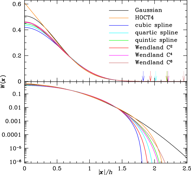
Figure 1: Kernels of Table 1, the Gaussian, and the HOCT4 kernel of Read et al. (2010) scaled to a common resolution scale of $h=2\sigma$ for 3D (top: linear plot, arrows indicating $|\boldsymbol{x}|=H$; bottom: logarithmic plot).

2.3 Kernel comparison

Fig. 1 plots the kernel functions $w(r)$ of Table 1, the Gaussian, and the HOCT4 kernel, all scaled to the same $h=2\sigma$ for $\nu=3$. Amongst the various scalings (ratios for $h/H$) discussed in §2.1 above, this gives by far the best match between the kernels. The B-splines and Wendland functions approach the Gaussian with increasing order. The most obvious difference between them in this scaling is their central value. The B-splines, in particular of lower order, put less emphasis on small $r$ than the Wendland functions or the Gaussian.

Obviously, the HOCT4 kernel, which has no inflection point, differs significantly from all the others and puts even more emphasis on the centre than the Gaussian (for this kernel $\sigma\approx 0.228343H$).

2.4 Kernel Fourier transforms

For spherical kernels of the form (6), their Fourier transform only depends on the product $H|\boldsymbol{k}|$, i.e. $\widehat{W}(\boldsymbol{k})=\widehat{w}(H|\boldsymbol{k}|)$. In 3D ($\mathcal{F}_{\nu}$ denotes the Fourier transform in $\nu$ dimensions)

$$\textstyle\widehat{w}(\kappa)=\mathcal{F}_{3}\left[w(r)\right](\kappa)=4\pi\kappa^{-1}\int_{0}^{\infty}\sin(\kappa r)\,w(r)\,r\,\mathrm{d}r$$ (14)

which is an even function and (up to a normalisation constant) equals $-\kappa^{-1}\mathrm{d}\mathcal{F}_{1}\big{[}w\big{]}/\mathrm{d}\kappa$. For the B-splines, which are defined via their 1D Fourier transform in equation (11), this gives immediately

$$\textstyle\mathcal{F}_{3}\left[b_{n}(r)\right](\kappa)=3\left(\frac{\textstyle n}{\textstyle\kappa}\right)^{n+2}\sin^{n}\!\frac{\textstyle\kappa}{\textstyle n}\left(1-\frac{\textstyle\kappa}{\textstyle n}\cot\frac{\textstyle\kappa}{\textstyle n}\right)$$ (15)

(which includes the normalisation constant), while for the 3D Wendland kernels

$$\mathcal{F}_{3}\left[\psi_{\ell k}(r)\right](\kappa)=\left(-\frac{1}{\kappa}\frac{\mathrm{d}}{\mathrm{d}\kappa}\right)^{k+1}\mathcal{F}_{1}\left[(1-r)^{\ell}_{+}\right](\kappa)$$ (16)

(we abstain from giving individual functional forms).

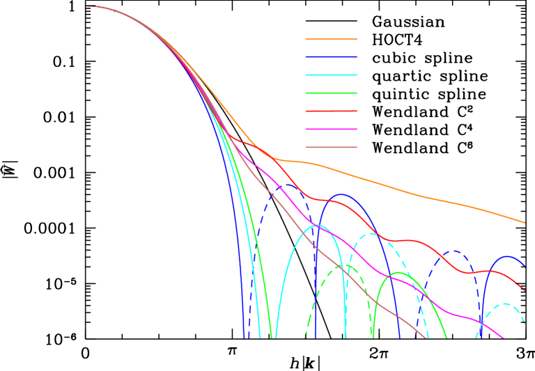
Figure 2: Fourier transforms $\widehat{W}(\boldsymbol{k})$ for the Gaussian, the HOCT4 and the kernels of Table 1 scaled to the same common scale $h=2\sigma$. Negative values are plotted with broken curves.

All these are plotted in Fig. 2 after scaling them to a common $h=2\sigma$. Notably, all the B-spline kernels obtain $\widehat{W}<0$ and oscillate about zero for large $\boldsymbol{k}$ (which can also be verified directly from equation 15), whereas the Wendland kernels have $\widehat{W}(\boldsymbol{k})>0$ at all $\boldsymbol{k}$, as does the HOCT4 kernel. As non-negativity of the Fourier transform is necessary (but not sufficient) for stability against pairing at large $N_{\!H}$ (see §3.1.2), in 3D the B-splines (of any order) fall prey to this instability for sufficiently large $N_{\!H}$, while, based solely on their Fourier transforms, the Wendland and HOCT4 kernels may well be stable for all neighbour numbers.

At large $|\boldsymbol{k}|$ (small scales), the HOCT kernel has most power, caused by its central spike, while the other kernels have ever less small-scale power with increasing order, becoming ever smoother and approaching the Gaussian, which has least small-scale power.

The scaling to a common $h=2\sigma$ in Fig. 2 has the effect that the $\widehat{W}(\boldsymbol{k})$ all overlap at small wave numbers, since their Taylor series

$$\widehat{W}(\boldsymbol{k})=1-\tfrac{1}{2}\sigma^{2}\boldsymbol{k}^{2}+\mathcal{O}(|\boldsymbol{k}|^{4}).$$ (17)

2.5 Density estimation and correction

The SPH force (3) is inseparably related, owing to its derivation via a variational principle, to the derivative of the density estimate. Another important role of the SPH density estimator is to obtain accurate values for $\hat{P}_{i}$ in equation (3), and we will now assess the performance of the various kernels in this latter respect.

In Fig. 3, we plot the estimated density (1) vs. neighbour number $N_{\!H}$ for the kernels of Table 1 and particles distributed in three-dimensional densest-sphere packing (solid curves) or a glass (squares). While the standard cubic spline kernel under-estimates the density (only values $N_{\!H}\lesssim 55$ are accessible for this kernel owing to the pairing instability), the Wendland kernels (and Gaussian, not shown) tend to over-estimate it.

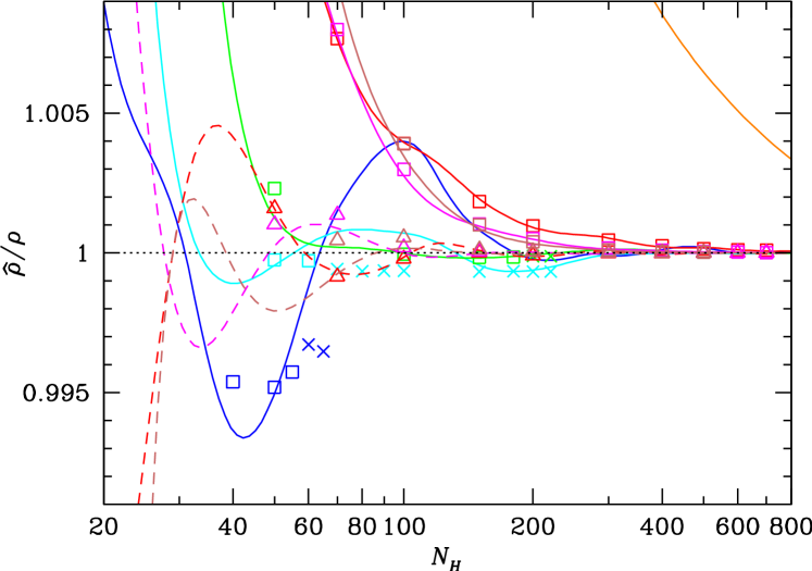
Figure 3: SPH density estimate (1) obtained from particles in three-dimensional densest-sphere packing (solid), glass (squares), or pairing (crosses), plotted against neighbour number $N_{\!H}$ for the kernels of Table 1 and the HOCT4 kernel (colour coding as in Figs. 1&2). For the Wendland kernels, the corrected density estimate (18) is shown with dashed curves and triangles for densest-sphere packing, and a glass, respectively.

It is worthwhile to ponder about the origin of this density over-estimation. If the particles were randomly rather than semi-regularly distributed, $\hat{\rho}$ obtained for an unoccupied position would be unbiased (e.g. Silverman, 1986), while at a particle position the self contribution $m_{i}W(0,h_{i})$ to $\hat{\rho}_{i}$ results in an over-estimate. Of course, in SPH and in Fig. 3 particles are not randomly distributed, but at small $N_{\!H}$ the self-contribution still induces some bias, as evident from the over-estimation for all kernels at very small $N_{\!H}$.

The HOCT4 kernel of Read et al. (2010, orange) with its central spike (cf. Fig. 1) shows by far the worst performance. However, this is not a peculiarity of the HOCT4 kernel, but a generic property of all kernels without inflection point.

These considerations suggest the corrected density estimate

$$\hat{\rho}_{i,\mathrm{corr}}=\hat{\rho}_{i}-\epsilon\,m_{i}\,W(0,h_{i}),$$ (18)

which is simply the original estimate (1) with a fraction $\epsilon$ of the self-contribution subtracted. The equations of motion obtained by replacing $\hat{\rho}_{i}$ in the Lagrangian (2) with $\hat{\rho}_{i,\mathrm{corr}}$ are otherwise identical to equations (3) and (4) (note that $\partial(\!h_{i}^{\nu}\hat{\rho}_{i,\mathrm{corr}})/\partial\ln h_{i}=\partial(\!h_{i}^{\nu}\hat{\rho}_{i})/\partial\ln h_{i}$, since $h_{i}^{\nu}\hat{\rho}_{i}$ and $h_{i}^{\nu}\hat{\rho}_{i,\mathrm{corr}}$ differ only by a constant), in particular the conservation properties are unaffected. From the data of Fig. 3, we find that good results are obtained by a simple power-law

$$\epsilon=\epsilon_{100}\,(N_{\!H}/100)^{-\alpha}$$ (19)

with constants $\epsilon_{100}$ and $\alpha$ depending on the kernel. We use $(\epsilon_{100},\alpha)$ = (0.0294, 0.977), (0.01342, 1.579), and (0.0116, 2.236), respectively, for the Wendland $C^{2}$, $C^{4}$, and $C^{6}$ kernels in $\nu=3$ dimensions.

The dashed curves and triangles in Fig. 3 demonstrate that this approach obtains accurate density and hence pressure estimates.

3 Linear stability and sound waves

The SPH linear stability analysis considers a plane-wave perturbation to an equilibrium configuration, i.e. the positions are perturbed according to

$$\boldsymbol{x}_{i}\to\boldsymbol{x}_{i}+\boldsymbol{a}\,\exp\big{(}i[\boldsymbol{k}{\cdot}\boldsymbol{x}_{i}-\omega t]\big{)}$$ (20)

with displacement amplitude $\boldsymbol{a}$, wave vector $\boldsymbol{k}$, and angular frequency $\omega$. Equating the forces generated by the perturbation to linear order in $\boldsymbol{a}$ to the acceleration of the perturbation yields a dispersion relation of the form

$$\boldsymbol{a}\cdot\boldsymbol{\mathsf{P}}(\boldsymbol{k})=\omega^{2}\boldsymbol{a}.$$ (21)

This is an eigenvalue problem for the matrix $\boldsymbol{\mathsf{P}}$ with eigenvector $\boldsymbol{a}$ and eigenvalue $\omega^{2}$. The exact (non-SPH) dispersion relation (with $c^{2}=\partial P/\partial\rho$, $P=\rho^{2}\partial u/\partial\rho$ at constant entropy)

$$c^{2}\,\boldsymbol{a}{\cdot}\boldsymbol{k}\,\boldsymbol{k}=\omega^{2}\boldsymbol{a}$$ (22)

has only one non-zero eigenvalue $\omega^{2}=c^{2}\boldsymbol{k}^{2}$ with eigenvector $\boldsymbol{a}\parallel\boldsymbol{k}$, corresponding to longitudinal sound waves propagating at speed $c$.

The actual matrix $\boldsymbol{\mathsf{P}}$ in equation (21) depends on the details of the SPH algorithm. For conservative SPH with equation of motion (3), Monaghan (2005) gives it for $P\propto\rho^{\gamma}$ in one spatial dimension. We derive it in appendix A for a general equation of state and any number $\nu$ of spatial dimensions:

$$\boldsymbol{\mathsf{P}}=\bar{c}^{2}\boldsymbol{u}^{(2)}+\frac{2\bar{P}}{\bar{\rho}}\left(\boldsymbol{\mathsf{U}}-\boldsymbol{u}^{(2)}+\!\left\{\frac{\bar{\Xi}}{2}\boldsymbol{u}^{(2)}-\frac{1}{2\nu\bar{\rho}^{2}\bar{\Omega}^{2}}\frac{\partial\boldsymbol{t}^{(2)}}{\partial\ln\!\bar{h}}\right\}\right),$$ (23)

where $\boldsymbol{x}^{(2)}$ is the outer product of a vector with itself, bars denote SPH estimates for the unperturbed equilibrium, $\boldsymbol{t}=\bar{\rho}\bar{\Omega}\boldsymbol{u}$, and

$$\boldsymbol{u}(\boldsymbol{k}) = \frac{1}{\bar{\rho}\{\bar{\Omega}\}}\sum_{j}m\sin\boldsymbol{k}{\cdot}\bar{\boldsymbol{x}}_{\!j}\,\boldsymbol{\nabla}W(\bar{\boldsymbol{x}}_{\!j},\bar{h}),$$ (24a)

$$\boldsymbol{\mathsf{U}}(\boldsymbol{k}) = \frac{1}{\bar{\rho}\{\bar{\Omega}\}}\sum_{j}m\,\big{(}1-\cos\boldsymbol{k}{\cdot}\bar{\boldsymbol{x}}_{\!j}\big{)}\,\boldsymbol{\nabla}^{(2)}W(\bar{\boldsymbol{x}}_{\!j},\bar{h}),$$ (24b)

$$\bar{\Xi} = \frac{1}{\nu}\frac{\partial\ln(\bar{\rho}\bar{\Omega})}{\partial\ln\bar{h}}\simeq 0.$$ (24c)

Here and in the remainder of this section, curly brackets indicate terms not present in the case of a constant $h=\bar{h}$, when our results reduce to relations given by Morris (1996) and Read et al. (2010).

Since $\boldsymbol{\mathsf{P}}$ is real and symmetric, its eigenvalues are real and its eigenvectors mutually orthogonal. The SPH dispersion relation (21) can deviate from the true relation (22) in mainly two ways. First, the longitudinal eigenvalue $\omega_{\scriptscriptstyle\parallel}^{2}$ (with eigenvector $\boldsymbol{a}_{\scriptscriptstyle\parallel}\parallel\boldsymbol{k}$) may deviate from $c^{2}\boldsymbol{k}^{2}$ (wrong sound speed) or even be negative (pairing instability; Morris 1996; Monaghan 2000). Second, the other two eigenvalues $\omega^{2}_{\perp 1,2}$ may be significantly non-zero (transverse instability for $\omega^{2}_{\perp 1,2}<0$ or transverse sound waves for $\omega^{2}_{\perp 1,2}>0$).

The matrix $\boldsymbol{\mathsf{P}}$ in equation (23) is not accessible to simple interpretation. We will compute its eigenvalues for the various SPH kernels in §​§3.2-3 and Figs. 4-6, but first consider the limiting cases of the dispersion relation, allowing some analytic insight.

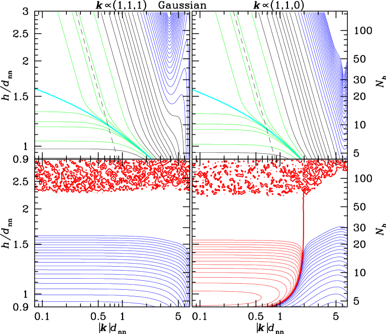
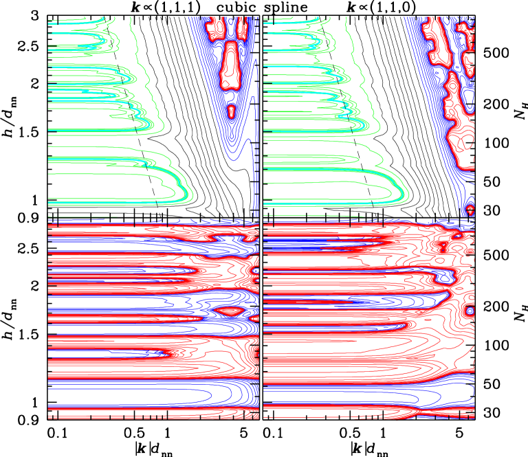
Figure 4: Stability of conservative SPH with the Gaussian (truncated at $16\sigma$) and cubic spline kernel for densest-sphere packing and $P\propto\rho^{5/3}$: contours of $\omega_{\scriptscriptstyle\parallel}^{2}/c^{2}\boldsymbol{k}^{2}$ (top) and $\omega^{2}_{\perp 2}/c^{2}\boldsymbol{k}^{2}$ (bottom), the longitudinal and smallest transverse eigenvalues of $\boldsymbol{\mathsf{P}}/c^{2}\boldsymbol{k}^{2}$ respectively, over wave number $|\boldsymbol{k}|$ and smoothing scale $h=2\sigma$ (and $N_{\!H}$ or $N_{\!h}$) both scaled to the nearest-neighbour distance $d_{\mathrm{nn}}$. The left and right sub-panels are for $\boldsymbol{k}\propto(1,1,1)$ (perpendicular to hexagonal planes), and $\boldsymbol{k}\propto(1,1,0)$ (nearest-neighbour direction), respectively (other wave vectors give similar results). Red contours are for $\omega^{2}\leq 0$ (implying the pairing instability in the top panels) and are logarithmically spaced by $0.25$ dex. Blue contours are also logarithmically spaced between $10^{-6}$ and $0.1$, black contours are linearly spaced by $0.1$, while good values for $\omega_{\scriptscriptstyle\parallel}^{2}$ are $\omega_{\scriptscriptstyle\parallel}^{2}/c^{2}\boldsymbol{k}^{2}=0.95$, 0.99, 0.995, 0.999, 1.001 1.005, 1.01, 1.05 (green), and 1 (cyan). The dashed line indicates a sound wave with wavelength $\lambda=8h=16\sigma$. For the Gaussian kernel $|\omega^{2}_{\perp 2}|$ in the bottom panels is often smaller than our numerical precision.

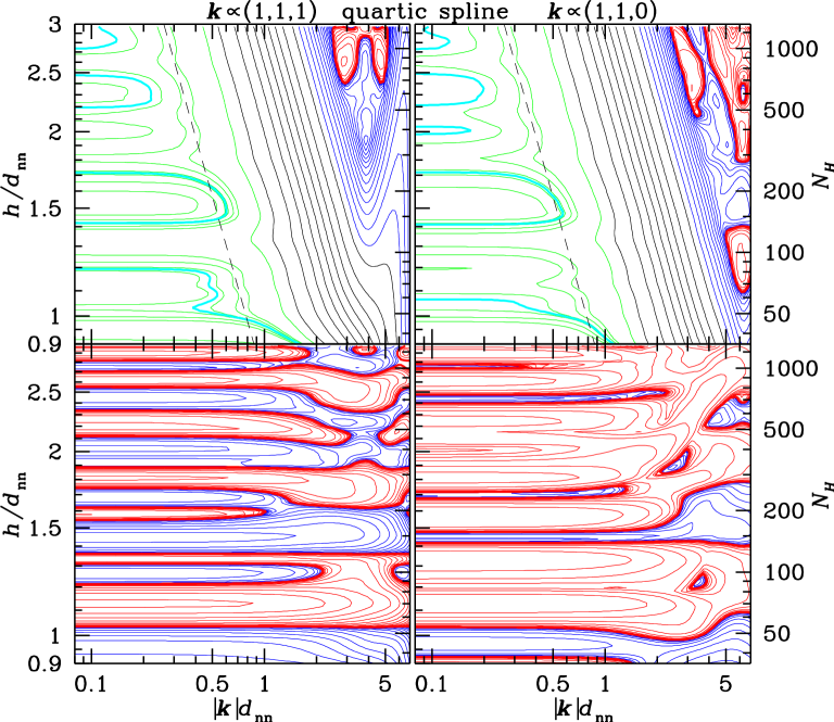
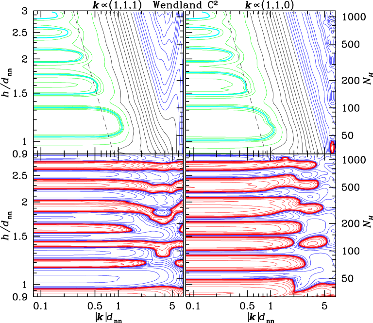
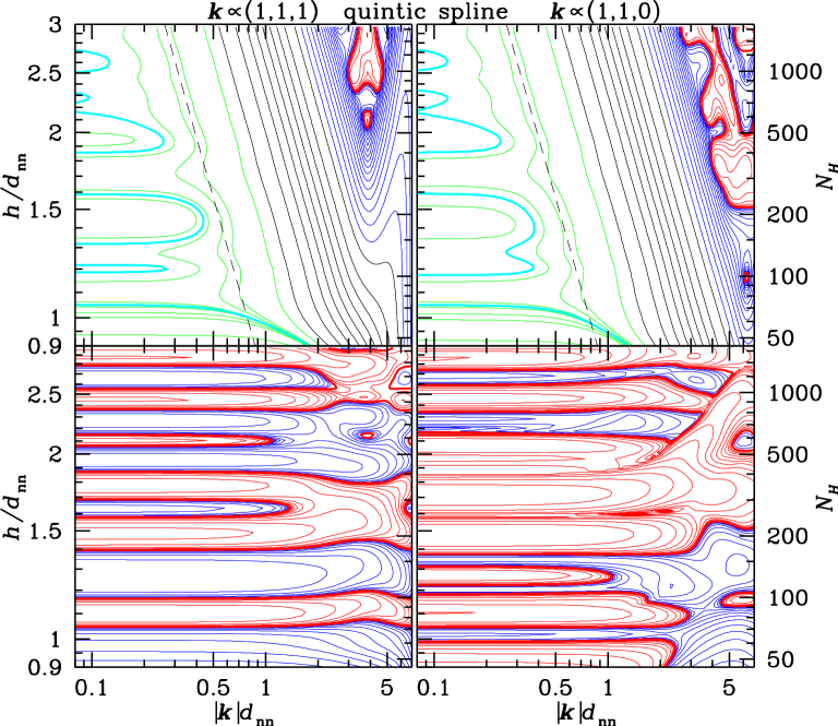
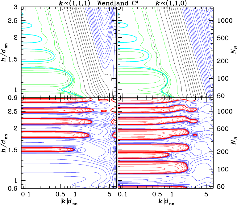
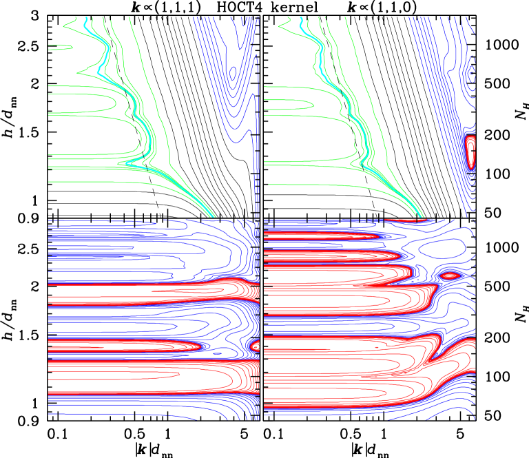
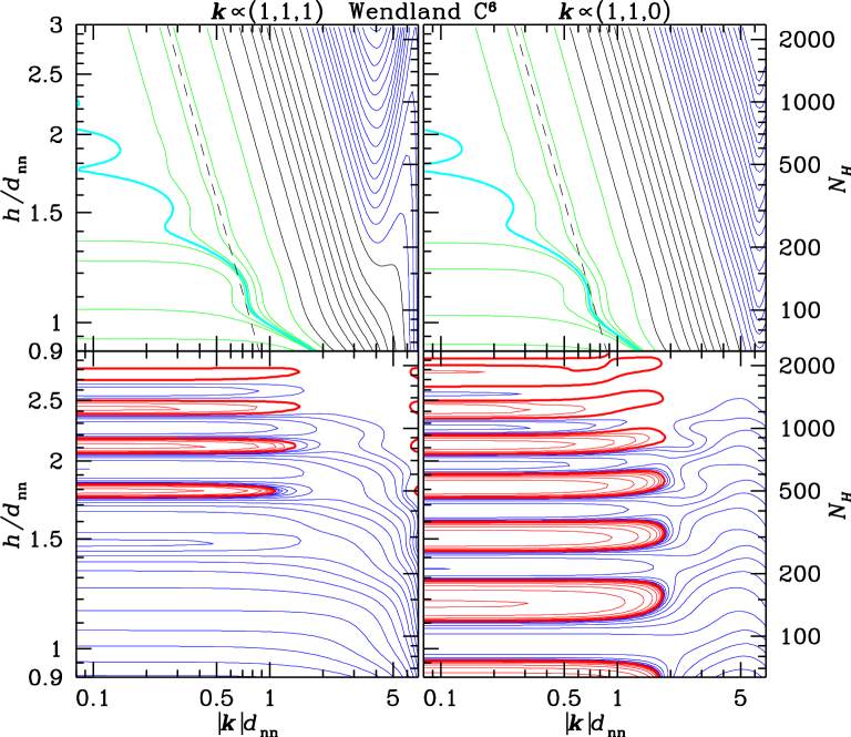
Figure 5: As Fig. 4, but for the quartic and quintic spline and the HOCT4 kernel (left) and the Wendland $C^{2}$ to $C^{6}$ kernels (right). The fine details of these contours are specific to the densest-sphere packing and will be different for more realistic glass-like particle distributions.

3.1 Limiting cases

There are three spatial scales: the wavelength $\lambda=2\pi/|\boldsymbol{k}|$, the smoothing scale $h$, and the nearest neighbour distance $d_{\mathrm{nn}}$. We will separately consider the limit $\lambda\gg h$ of well resolved waves, the continuum limit $h\gg d_{\mathrm{nn}}$ of large neighbour numbers, and finally the combined limit $\lambda\gg h\gg d_{\mathrm{nn}}$.

3.1.1 Resolved waves

If $|\boldsymbol{k}|h\ll 1$, the argument of the trigonometric functions in equations (24a,b) is always small and we can Taylor expand them. If we also assume a locally isotropic particle distribution, this gives to lowest order in $|\boldsymbol{k}|$ ($\boldsymbol{\mathsf{I}}$ is the unit matrix; see also §A.3)

$$\boldsymbol{\mathsf{P}}\to\bar{c}^{2}\boldsymbol{k}^{(2)}+\bar{\Xi}\,\frac{\bar{P}}{\bar{\rho}}\left[\left(\frac{2\nu}{\nu+2}-\{1\}\right)\boldsymbol{k}^{(2)}+\frac{\nu\boldsymbol{k}^{2}}{\nu+2}\,\boldsymbol{\mathsf{I}}\right]$$ (25)

with the eigenvalues

$$\frac{\omega_{\scriptscriptstyle\parallel}^{2}}{\boldsymbol{k}^{2}} = \bar{c}^{2}+\bar{\Xi}\,\frac{\bar{P}}{\bar{\rho}}\left(\frac{3\nu}{\nu+2}-\{1\}\right),$$ (26a)

$$\frac{\omega_{\perp 1,2}^{2}}{\boldsymbol{k}^{2}} = \bar{\Xi}\,\frac{\bar{P}}{\bar{\rho}}\frac{\nu}{\nu+2}.$$ (26b)

The error of these relations is mostly dictated by the quality of the density estimate, either directly via $\bar{\rho}$, $\bar{c}$, and $\bar{P}$, or indirectly via $\bar{\Xi}$. The density correction method of equation (18) can only help with the former, but not the latter. The difference between constant and adapted $h$ is a factor 4/9 (for 3D) in favour of the latter.

3.1.2 Continuum limit

For large neighbour numbers $N_{\!H}$, $H\gg d_{\mathrm{nn}}$, $\bar{\Omega}\&\bar{\Pi}\to 1$, $\bar{\rho}\to\rho$ and the sums in equations (24a,b) can be approximated by integrals

$$\boldsymbol{u}\to-\boldsymbol{k}\,\widehat{W}(\boldsymbol{k}),\;\;\text{and}\;\;\boldsymbol{\mathsf{U}}\to\boldsymbol{k}^{(2)}\,\widehat{W}(\boldsymbol{k}),$$ (27)

with $\widehat{W}(\boldsymbol{k})$ the Fourier transform of $W(\boldsymbol{x},h)$. Since $\widehat{W}(\boldsymbol{k})=\widehat{w}(H|\boldsymbol{k}|)$, we have $\partial\widehat{W}/\partial\ln h=\boldsymbol{k}{\cdot}\boldsymbol{\nabla}_{\!k}\widehat{W}$ and thus from equation (23)

$$\boldsymbol{\mathsf{P}}\to c^{2}\boldsymbol{k}^{(2)}\,\widehat{W}\left[\widehat{W}+\frac{2P}{\rho c^{2}}\bigg{(}1-\widehat{W}-\left\{\nu^{-1}\boldsymbol{k}{\cdot}\boldsymbol{\nabla}_{\!k}\widehat{W}\right\}\bigg{)}\right].$$ (28)

$\widehat{W}(0)=1$, but towards larger $|\boldsymbol{k}|$ the Fourier transform decays, $\widehat{W}(\boldsymbol{k})<1$, and in the limit $h|\boldsymbol{k}|\gg 1$ or $\lambda\ll h$, $\widehat{W}\to 0$: short sound waves are not resolved.

Negative eigenvalues of $\boldsymbol{\mathsf{P}}$ in equation (28), and hence linear instability, occur only if $\widehat{W}$ itself or the expression within square brackets are negative. Since $\widehat{W}\leq 1$, the latter can only happen if $P<0$, which does usually not arise in fluid simulations (unless, possibly, one subtracts an average pressure), but possibly in elasticity simulations of solids (Gray, Monaghan & Swift, 2001), when it causes the tensile instability (an equivalent effect is present in smoothed-particle MHD, see Phillips & Monaghan 1985; Price 2012). Monaghan (2000) proposed an artificial repulsive short-range force, effectuating an additional pressure, to suppress the tensile instability.

The pairing instability, on the other hand, is caused by $\widehat{W}<0$ for some $H|\boldsymbol{k}|>\kappa_{0}$. This instability can be avoided by choosing the neighbour number $N_{\!H}$ small enough for the critical wave number $\kappa_{0}$ to remain unsampled, i.e. $\kappa_{0}>\kappa_{\mathrm{Nyquist}}$ or $H\lesssim d_{\mathrm{nn}}\kappa_{0}/\pi$ (though such small $H$ is no longer consistent with the continuum limit).

However, if the Fourier transform of the kernel is non-negative everywhere, the pairing instability cannot occur for large $N_{\!H}$. As pairing is typically a problem for large $N_{\!H}$, this suggests that kernels with $\widehat{W}(\boldsymbol{k})>0$ for every $\boldsymbol{k}$ are stable against pairing for all values of $N_{\!H}$, which is indeed supported by our results in §4.1.

3.1.3 Resolved waves in the continuum limit

The combined limit of $\lambda\gg h\gg d_{\mathrm{nn}}$ is obtained by inserting the Taylor expansion (17) of $\widehat{W}$ into equation (28), giving

$$\omega_{\scriptscriptstyle\parallel}^{2}=c^{2}\boldsymbol{k}^{2}\left(1+\sigma^{2}\boldsymbol{k}^{2}\gamma^{-1}\big{[}\left\{2/\nu\right\}+1-\gamma\big{]}+\mathcal{O}(h^{4}|\boldsymbol{k}|^{4})\right).$$ (29)

Monaghan (2005) gave an equivalent relation for $\nu=1$ when the expression in square brackets becomes $3-\gamma$ or $1-\gamma$ (for adapted or constant $h$, respectively), which, he argues, bracket all physically reasonable values. However, in 3D the value for adaptive SPH becomes $5/3-\gamma$, i.e. vanishes for the most commonly used adiabatic index.

In general, however, the relative error in the frequency is $\propto\sigma^{2}\boldsymbol{k}^{2}\propto(\sigma/\lambda)^{2}$. This shows that $h=2\sigma$ is indeed directly proportional to the resolution scale, at least concerning sound waves.

3.2 Linear stability of SPH kernels

We have evaluated the eigenvalues $\omega_{\scriptscriptstyle\parallel}^{2}$ and $\omega_{\perp 1,2}^{2}$ of the matrix $\boldsymbol{\mathsf{P}}$ in equation (23) for all kernels of Table 1, as well as the HOCT4 and Gaussian kernels, for unperturbed positions from densest-sphere packing (face-centred cubic grid). In Figs. 4&5, we plot the resulting contours of $\omega^{2}\!/\!c^{2}\boldsymbol{k}^{2}$ over wave number $|\boldsymbol{k}|$ and smoothing scale $h$ (both normalised by the nearest-neighbour distance $d_{\mathrm{nn}}$) or $N_{\!H}$ on the right axes (except for the Gaussian kernel when $N_{\!H}$ is ill-defined and we give $N_{\!h}$ instead) for two wave directions, one being a nearest-neighbour direction.

3.2.1 Linear stability against pairing

The top sub-panels of Figs. 4&5 refer to the longitudinal eigenvalue $\omega_{\scriptscriptstyle\parallel}^{2}$, when green and red contours are for, respectively, $\omega_{\scriptscriptstyle\parallel}^{2}\approx c^{2}\boldsymbol{k}^{2}$ and $\omega_{\scriptscriptstyle\parallel}^{2}<0$, the latter indicative of the pairing instability. For the Gaussian kernel (truncated at $16\sigma$; Fig. 4) $\omega_{\scriptscriptstyle\parallel}^{2}>0$ everywhere, proving its stability, similar to the HOCT4 and, in particular the higher-degree, Wendland kernels. In contrast, all the B-spline kernels obtain $\omega_{\scriptscriptstyle\parallel}^{2}<0$ at sufficiently large $N_{\!H}$.

The quintic spline, Wendland $C^{2}$, and HOCT4 kernel each have a region of $\omega_{\scriptscriptstyle\parallel}^{2}<0$ for $|\boldsymbol{k}|$ close to the Nyquist frequency and $N_{\!H}\approx 100$, $N_{\!H}\approx 40$, and $N_{\!H}\sim 150$, respectively. In numerical experiments similar to those described in §4.1, the corresponding instability for the quintic spline and Wendland $C^{2}$ kernels can be triggered by very small random perturbations to the grid equilibrium. However, such modes are absent in glass-like configurations, which naturally emerge by ‘cooling’ initially random distributions. This strongly suggests, that these kernel-$N_{\!H}$ combinations can be safely used in practice. Whether this also applies to the HOCT4 kernel at $N_{\!H}\sim 150$ we cannot say, as we have not run test simulations for this kernel. Note, that these islands of linear instability at small $N_{\!H}$ are not in contradiction to the relation between kernel Fourier transform and stability and are quite different from the situation for the B-splines, which are only stable for sufficiently small $N_{\!H}$.

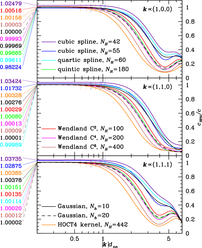
Figure 6: Ratio of SPH sound speed $c_{\mathrm{SPH}}=\omega_{\scriptscriptstyle\parallel}/|\boldsymbol{k}|$ for the equation of state $P\propto\rho^{5/3}$ to the correct $c$ for the kernel-$N_{\!H}$ combinations of Table 2 and three different wave directions (as indicated) for particles in densest-sphere packing with nearest-neighbour separation $d_{\mathrm{nn}}$. These curves are horizontal cuts through the top panels of Figs. 4&5. The thin vertical lines indicate sound with wavelength $\lambda=8h$, corresponding to the dashed lines in Figs. 4&5.

3.2.2 Linear transverse instability?

The bottom sub-panels of Figs. 4&5 show $\omega_{\perp 2}^{2}/c^{2}\boldsymbol{k}^{2}$, when both families of kernels have $0\approx|\omega_{\perp 1,2}^{2}|\ll c^{2}\boldsymbol{k}^{2}$ with either sign occurring. $\omega_{\perp 1,2}^{2}<0$ implies growing transverse modes, which we indeed found in simulations starting from a slightly perturbed densest-sphere packing. However, such modes are not present in glass-like configurations, which strongly suggests, that transverse modes are not a problem in practice.

3.3 Numerical resolution of sound waves

The dashed lines in Figs. 4&5 indicate sound with wavelength $\lambda=8h$. For $h\gtrsim d_{\mathrm{nn}}$, such sound waves are well resolved in the sense that the sound speed is accurate to $\lesssim 1\%$. This is similar to grid methods, which typically require about eight cells to resolve a wavelength.

The effective SPH sound speed can be defined as $c_{\mathrm{SPH}}=\omega_{\scriptscriptstyle\parallel}/|\boldsymbol{k}|$. In Fig. 6 we plot the ratio between $c_{\mathrm{SPH}}$ and the correct sound speed as function of wave number for three different wave directions and the ten kernel-$N_{\!H}$ combinations of Table 2 (which also gives their formal resolutions). The transition from $c_{\mathrm{SPH}}\approx c$ for long waves to $c_{\mathrm{SPH}}\ll c$ for short waves occurs at $|\boldsymbol{k}|d_{\mathrm{nn}}\gtrsim 1$, but towards longer waves for larger $h/d_{\mathrm{nn}}$, as expected.

For resolved waves ($\lambda\gtrsim 8h$: left of the thin vertical lines in Fig. 6), $c_{\mathrm{SPH}}$ obtains a value close to $c$, but with clear differences between the various kernel-$N_{\!H}$ combinations. Surprisingly, the standard cubic spline kernel, which is used almost exclusively in astrophysics, performs very poorly with errors of few percent, for both $N_{\!H}=42$ and 55. This is in stark contrast to the quartic spline with similar $N_{\!H}=60$ but $c_{\mathrm{SPH}}$ accurate to $<1\%$. Moreover, the quartic spline with $N_{\!H}=60$ resolves shorter waves better than the cubic spline with a smaller $N_{\!H}=55$, in agreement with Table 2.

We should note that these results for the numerical sound speed assume a perfectly smooth simulated flow. In practice, particle disorder degrades the performance, in particular for smaller $N_{\!H}$, and the resolution of SPH is limited by the need to suppress this degradation via increasing $h$ (and $N_{\!H}$).

kernel	$N_{\!H}$	$N_{\!h}$	$h/d_{\mathrm{nn}}$	$h(\hat{\rho}/m)^{1/3}$
cubic spline	42	6.90	1.052	1.181
cubic spline	55	9.04	1.151	1.292
quartic spline	60	7.29	1.072	1.203
quintic spline	180	17.00	1.421	1.595
Wendland $C^{2}$	100	13.77	1.325	1.487
Wendland $C^{4}$	200	18.58	1.464	1.643
Wendland $C^{6}$	400	27.22	1.662	1.866
HOCT4	442	42.10	1.923	2.158
Gaussian	$\infty$	10.00	1.191	1.337
Gaussian	$\infty$	20.00	1.500	1.684

Table 2: Some quantities (defined in §2.1) for kernel-$N_{\!H}$ combinations used in Fig. 6 and the test simulations of §4. $d_{\mathrm{nn}}$ is the nearest-neighbour distance for densest-sphere packing, which has number density $n=\!\sqrt{2}\,d_{\mathrm{nn}}^{-3}$. The cubic spline with $N_{\!H}\approx 42$ is the most common choice in astrophysical simulations, the other $N_{\!H}$ values for the B-spline are near the pairing-stability boundary, hence obtaining close to the greatest possible reduction of the ‘E₀ errors’. For $N_{\!H}=100$, 200, 400, we picked the Wendland kernel which gave best results for the vortex test of §4.2.

4 Test simulations

In order to assess the Wendland kernels and compare them to the standard B-spline kernels in practice, we present some test simulations which emphasise the pairing, strong shear, and shocks. All these simulations are done in 3D using periodic boundary conditions, $P=K\rho^{5/3}$, conservative SPH (equation 3), and the Cullen & Dehnen (2010) artificial viscosity treatment, which invokes dissipation only for compressive flows, and an artificial conductivity similar to that of Read & Hayfield (2012). For some tests we used various values of $N_{\!H}$ per kernel, but mostly those listed in Table 2.

4.1 Pairing in practice

In order to test our theoretical predictions regarding the pairing instability, we evolve noisy initial conditions with 32000 particles until equilibrium is reached. Initially, $\dot{\boldsymbol{x}}_{i}=0$, while the initial $\boldsymbol{x}_{i}$ are generated from densest-sphere packing by adding normally distributed offsets with (1D) standard deviation of one unperturbed nearest-neighbour distance $d_{\mathrm{nn}}$. To enable a uniform-density equilibrium (a glass), we suppress viscous heating.

The typical outcome of these simulations is either a glass-like configuration (right panel of Fig. 7) or a distribution with particle pairs (left panel of Fig. 7). In order to quantify these outcomes, we compute for each particle the ratio

$$r_{\min,i}=\min_{j\neq i}\big{\{}|\boldsymbol{x}_{i}-\boldsymbol{x}_{\!j}|\big{\}}/H_{i}$$ (30)

between its actual nearest-neighbour distance and kernel-support radius. The maximum possible value for $r_{\min}$ occurs for densest-sphere packing, when $|\boldsymbol{x}_{i}-\boldsymbol{x}_{\!j}|\geq d_{\mathrm{nn}}=(n/\!\sqrt{2})^{1/3}$ with $n$ the number density. Replacing $\hat{\rho}_{i}$ in equation (7) with $m_{i}n$, we obtain

$$r_{\min}\lesssim\big{(}3N_{\!H}/2^{5/2}\pi\big{)}^{1/3}.$$ (31)

Thus, the ratio

$$q_{\min,i}=\frac{r_{\min,i}}{(3N_{\!H}/2^{5/2}\pi)^{1/3}}\approx\min_{j\neq i}\left\{\frac{|\boldsymbol{x}_{i}-\boldsymbol{x}_{\!j}|}{d_{\mathrm{nn,grid}}}\right\}$$ (32)

is an indicator for the regularity of the particle distribution around particle $i$. It obtains a value very close to one for perfect densest-sphere packing and near zero for pairing, while a glass typically gives $q_{\min,i}\sim 0.7$.

Fig. 8 plots the final value for the overall minimum of $q_{\min,i}$ for each of a set of simulations. For all values tested for $N_{\!H}$ (up to 700), the Wendland kernels show no indication of a single particle pair. This is in stark contrast to the B-spline kernels, all of which suffer from particle pairing. The pairing occurs at $N_{\!H}>67$ and 190 for the quartic, and quintic spline, respectively, whereas for the cubic spline $\min_{i}\{q_{\min,i}\}$ approaches zero more gradually, with $\min_{i}\{q_{\min,i}\}\leq 0.16$ at $N_{\!H}>55$. These thresholds match quite well the suggestions of the linear stability analysis in Figs. 4&5 (except that the indications of instability of the quintic spline at $N_{\!H}\approx 100$ and the Wendland $C^{2}$ kernel at $N_{\!H}\approx 40$ are not reflected in our tests here). The quintic (and higher-order) splines are the only option amongst the B-spline kernels for $N_{\!H}$ appreciably larger than ${\sim\,}50$.

Figure 7: Final $x$ and $y$ positions for particles at $|z|<d_{\mathrm{nn}}/2$ for the tests of §4.1. Symbol size is linear in $z$: two overlapping symbols of the same size indicate particle pairing.

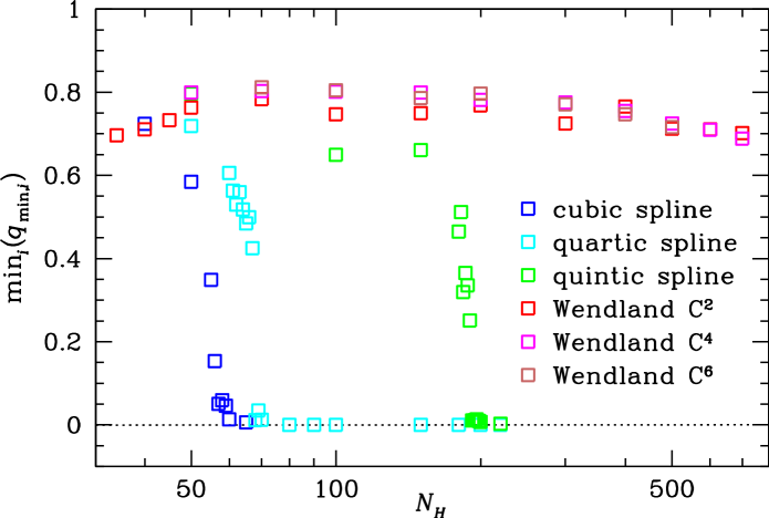
Figure 8: Final value of the overall minimum of $q_{\min,i}$ (equation 32) for simulations starting from noisy initial conditions for all kernels of Table 1 (same colour coding as in Fig. 3; using the density correction of §2.5 for the Wendland kernels) as function of $N_{\!H}$. For densest-sphere packing $q_{\min,i}\approx 1$, for a glass $0\ll q_{\min,i}<1$, while $q_{\min,i}\sim 0$ indicates particle pairing.

We also note that $\min_{i}\{q_{\min,i}\}$ grows substantially faster, in particularly early on, for the Wendland kernels than for the B-splines, especially when operating close to the stability boundary.

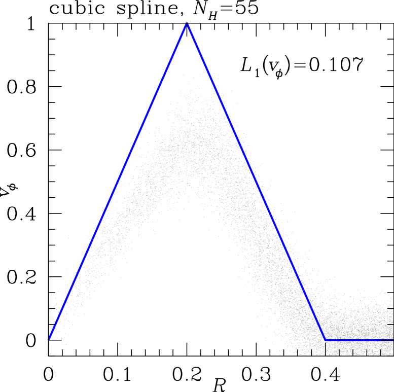
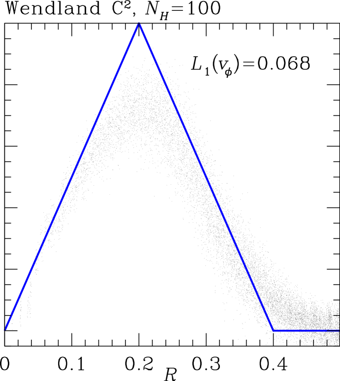
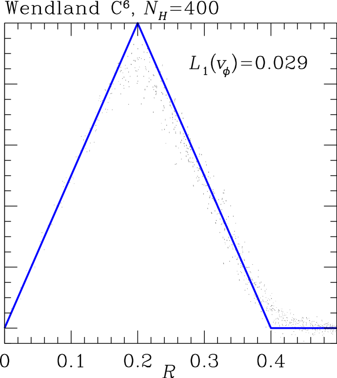
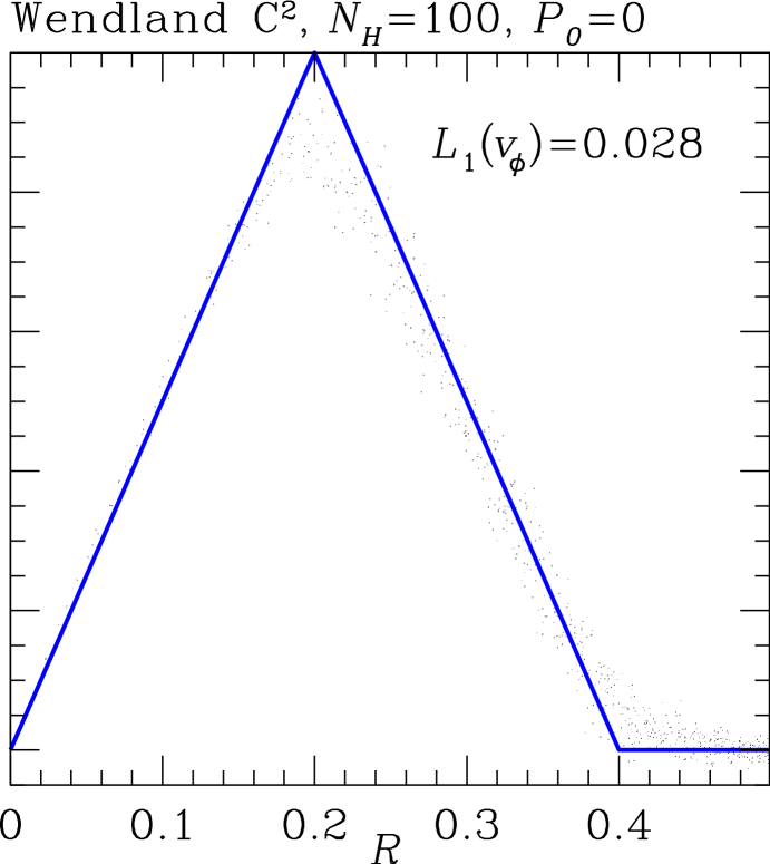
Figure 9: Velocity profiles the Gresho-Chan vortex test at time $t=1$ with the lowest resolution of $N_{\mathrm{1D}}=50.8$ for three different kernel-$N_{\!H}$ pairs (as indicated) and one simulation (right panel) with $P_{0}=0$ in equation (33d), when the ‘E₀ error’ is naturally much weaker. Only particles at $|z|<0.05$ are plotted.

4.2 The Gresho-Chan vortex test

As discussed in the introduction, particle disorder is unavoidably generated in shearing flows, inducing ‘E₀ errors’ in the forces and causing modelling errors. A critical test of this situation consists of a differentially rotating fluid of uniform density in centrifugal balance (Gresho & Chan 1990, see also Liska & Wendroff 2003, Springel 2010, and Read & Hayfield 2012). The pressure and azimuthal velocity are

$$P = \left\{\begin{array}[]{l@{\quad\text{for}\;\;}lllll}P_{0}+12.5R^{2}&0&\leq&R&<&0.2,\\ P_{0}+12.5R^{2}+4-20R+4\ln(5R)&0.2&\leq&R&<&0.4,\\ P_{0}+2(2\ln 2-1)&0.4&\leq&R&;&\end{array}\right.$$ (33d)

$$v_{\phi} = \left\{\begin{array}[]{l@{\quad\text{for}\;\;}lllll}5R&0&\leq&R&<&0.2,\\ 2-5R&0.2&\leq&R&<&0.4,\\ 0&0.4&\leq&R&&\end{array}\right.$$ (33h)

with $P_{0}=5$ and $R$ the cylindrical radius. We start our simulations from densest-sphere packing with effective one-dimensional particle numbers $N_{\mathrm{1D}}=51$, 102, 203, or 406. The initial velocities and pressure are set as in equations (33).

There are three different causes for errors in this test. First, an overly viscous method reduces the differential rotation, as shown by Springel (2010); this effect is absent from our simulations owing to the usage of the Cullen & Dehnen (2010) dissipation switch. Second, the ‘E₀ error’ generates noise in the velocities which in turn triggers some viscosity. Finally, finite resolution implies that the sharp velocity kinks at $R=0.2$ and 0.4 cannot be fully resolved (in fact, the initial conditions are not in SPH equilibrium because the pressure gradient at these points is smoothed such that the SPH acceleration is not exactly balanced with the centrifugal force).

In Fig. 9 we plot the azimuthal velocity at time $t=1$ for a subset of all particles at our lowest resolution of $N_{\mathrm{1D}}=51$ for four different kernel-$N_{\!H}$ combinations. The leftmost is the standard cubic spline with $N_{\!H}=55$, which considerably suffers from particle disorder and hence ‘E₀ errors (but also obtains too low $v_{\phi}$ at $R<0.2$).

The second is the Wendland $C^{2}$ kernel with $N_{\!H}=100$, which still suffers from the ‘E₀ error’. The last two are for the Wendland $C^{6}$ kernel with $N_{\!H}=400$ and the Wendland $C^{2}$ kernel with $N_{\!H}=100$ but with $P_{0}=0$ in equation (33d). In both cases, the ‘E₀ error’ is much reduced (and the accuracy limited by resolution) either because of large neighbour number or because of a reduced pressure.

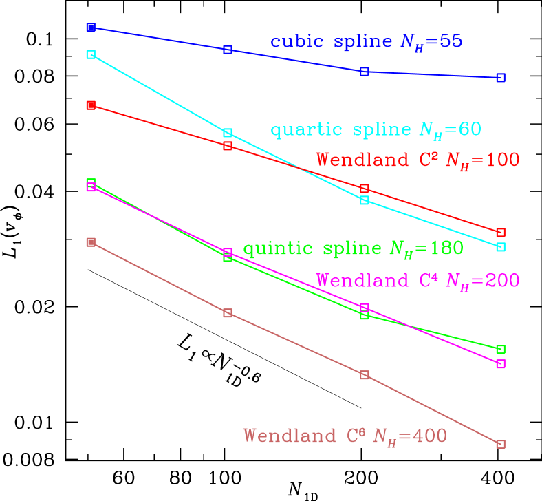
Figure 10: Convergence of the $L_{1}$ velocity error for the Gresho-Chan test with increasing number of particles (for a cubic lattice $N_{\mathrm{1D}}$ equals the number of cells along one side of the computational domain) for various kernel-$N_{\!H}$ combinations (those with filled squares are shown in Fig. 9). A comparison with Fig. 6 of Read & Hayfield (2012) shows that the Wendland $C^{6}$ kernel with $N_{\!H}=400$ performs better than the HOCT4 kernel with $N_{\!H}=442$.

​ ​ ​ ​ ​

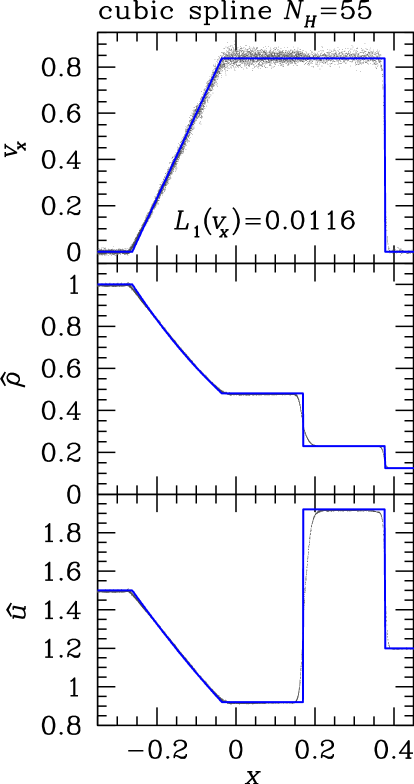
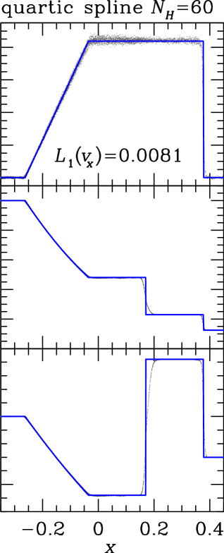
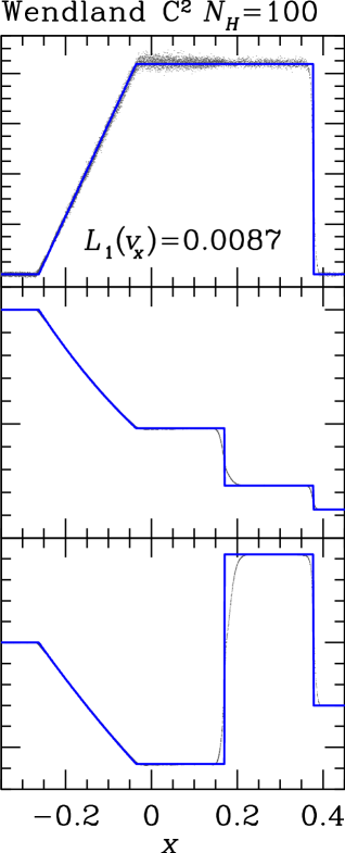
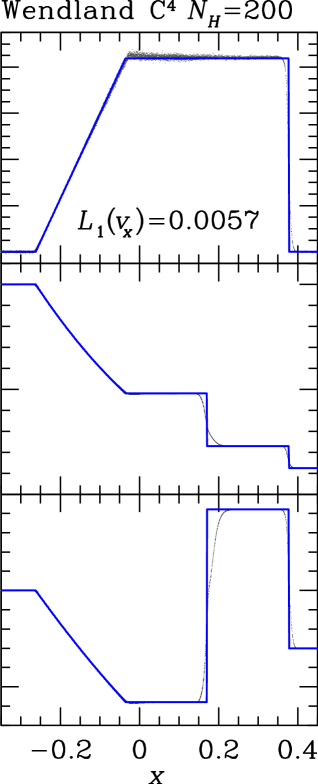
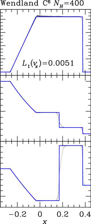
Figure 11: Velocity, density, and thermal energy profiles for the shock tube test at $t=0.2$ for the same kernel-$N_{\!H}$ combinations as in Fig. 10 in order of increasing $N_{\!H}$ (points: particles at $|y|,|z|<0.005$) and the exact solutions (solid). The $L_{1}$ velocity errors reported are computed for the range $-0.4<x<0.5$.

In Fig. 10, we plot the convergence of the $L_{1}$ velocity error with increasing numerical resolution for all the kernels of Table 1, but with another $N_{\!H}$ for each, see also Table 2. For the B-splines, we pick a large $N_{\!H}$ which still gives sufficient stability against pairing, while for $N_{\!H}=100$, 200, and 400 we show the Wendland kernel that gave best results. For the cubic spline, the results agree with the no-viscosity case in Fig. 6 of Springel (2010), demonstrating that our dissipation switch effectively yields inviscid SPH. We also see that the rate of convergence (the slope of the various curves) is lower for the cubic spline than any other kernel. This is caused by systematically too low $v_{\phi}$ in the rigidly rotating part at $R<0.2$ (see leftmost panel if Fig. 9) at all resolutions. The good performance of the quartic spline is quite surprising, in particular given the rather low $N_{\!H}$. The quintic spline at $N_{\!H}=180$ and the Wendland $C^{4}$ kernel at $N_{\!H}=200$ obtain very similar convergence, but are clearly topped by the Wendland $C^{6}$ kernel at $N_{\!H}=400$, demonstrating that high neighbour number is really helpful in strong shear flows.

4.3 Shocks

Our final test is the classical Sod (1978) shock tube, a 1D Riemann problem, corresponding to an initial discontinuity in density and pressure. Unlike most published applications of this test, we perform 3D simulations with glass-like initial conditions. Our objective here is (1) to verify the ‘E₀-error’ reductions at larger $N_{\!H}$ and (2) the resulting trade-off with the resolution across the shock and contact discontinuities. Other than for the vortex tests of §4.2, we only consider one value for the number $N$ of particles but the same six kernel-$N_{\!H}$ combinations as in Fig. 10. The resulting profiles of velocity, density, and thermal energy are plotted in Fig. 11 together with the exact solutions.

Note that the usual over-shooting of the thermal energy near the contact discontinuity (at $x=0.17$) is prevented by our artificial conductivity treatment. This is not optimised and likely over-smoothes the thermal energy (and with it the density). However, here we concentrate on the velocity.

For the cubic spline with $N_{\!H}=55$, there is significant velocity noise in the post-shock region. This is caused by the re-ordering of the particle positions after the particle distribution becomes anisotropically compressed in the shock. This type of noise is a well-known issue with multi-dimensional SPH simulations of shocks (e.g. Springel, 2010; Price, 2012). With increasing $N_{\!H}$ the velocity noise is reduced, but because of the smoothing of the velocity jump at the shock (at $x=0.378$) the $L_{1}$ velocity error does not approach zero for large $N_{\!H}$.

Instead, for sufficiently large $N_{\!H}$ ($\gtrsim 200$ in this test), the $L_{1}$ velocity error saturates: any ‘E₀-error’ reduction for larger $N_{\!H}$ is balanced by a loss of resolution. The only disadvantage of larger $N_{\!H}$ is an increased computational cost (by a factor $\sim 1.5$ when moving from the quintic spline with $N_{\!H}=180$ to the Wendland kernel $C^{6}$ with $N_{\!H}=400$, see Fig. 12).

5 Discussion

5.1 What causes the pairing instability?

The Wendland kernels have an inflection point and yet show no signs of the pairing instability. This clearly demonstrates that the traditional ideas for the origin of this instability (á la Swegle et al. 1995, see the introduction) were incorrect. Instead, our linear stability analysis shows that in the limit of large $N_{\!H}$ pairing is caused by a negative kernel Fourier transform $\widehat{W}$, whereas the related tensile instability with the same symptoms is caused by an (effective) negative pressure. While it is intuitively clear that negative pressure causes pairing, the effect of $\widehat{W}<0$ is less obvious. Therefore, we now provide another explanation, not restricted to large $N_{\!H}$.

5.1.1 The pairing instability as artifact of the density estimator

By their derivation from the Lagrangian (2), the SPH forces $m_{i}\ddot{\boldsymbol{x}}_{i}=\partial\mathcal{L}/\partial\boldsymbol{x}_{i}=-\partial\hat{U}\!/\partial\boldsymbol{x}_{i}$ tend to reduce the estimated total thermal energy $\hat{U}=\sum_{i}m_{i}\,u(\hat{\rho}_{i},s_{i})$ at fixed entropy. Thus, hydrostatic equilibrium corresponds to an extremum of $\hat{U}$, and stable equilibrium to a minimum when small positional changes meet opposing forces. Minimal $\hat{U}$ is obtained for uniform $\hat{\rho}_{i}$, since a re-distribution of the particles in the same volume but with a spread of $\hat{\rho}_{i}$ gives larger $\hat{U}$ (assuming uniform $s_{i}$). An equilibrium is meta-stable, if $\hat{U}$ is only a local (but not the global) minimum. Several extrema can occur if different particle distributions, each obtaining (near-)uniform $\hat{\rho}_{i}$, have different average $\hat{\rho}$. Consider, for example, particles in densest-sphere packing, replace each by a pair and increase the spacing by $2^{1/3}$, so that the average density $\rho$ (but not $\hat{\rho}$) remains unchanged. This fully paired distribution is in equilibrium with uniform $\hat{\rho}_{i}$, but the effective neighbour number is reduced by a factor 2 (for the same smoothing scale). Now if $\hat{\rho}(N_{\!H}/2)<\hat{\rho}(N_{\!H})$, the paired distribution has lower $\hat{U}$ than the original and is favoured.

In practice (and in our simulations in §4.1), the pairing instability appears gradually: for $N_{\!H}$ just beyond the stability boundary, only few particle pairs form and the effective reduction of $N_{\!H}$ is by a factor $f\leq 2$. We conclude, therefore, that

pairing occurs if $\hat{\rho}(N_{\!H}/f)<\hat{\rho}(N_{\!H})$ for some $1<f\leq 2$.

From Fig. 3 we see that for the B-spline kernels $\hat{\rho}(N_{\!H})$ always has a minimum and hence satisfies our condition, while this never occurs for the Wendland or HOCT4 kernels. The stability boundary (between squares and crosses in Fig. 3) is towards slightly larger $N_{\!H}$ than the minimum of $\hat{\rho}(N_{\!H})$, indicating $f>1$ (but also note that the curves are based on a regular grid instead of a glass as the squares).

5.1.2 The relation to ‘E₀ errors’ and particle re-ordering

A disordered particle distribution is typically not in equilibrium, but has non-uniform $\hat{\rho}_{i}$ and hence non-minimal $\hat{U}$. The SPH forces, in particular their ‘E₀ errors’ (which occur even for constant pressure), then drive the evolution towards smaller $\hat{U}$ and hence equilibrium with either a glass-like order or pairing (see also Price, 2012, §5). Thus, the minimisation of $\hat{U}\!$ is the underlying driver for both the particle re-ordering capability of SPH and the pairing instability. This also means that when operating near the stability boundary, for example using $N_{\!H}=55$ for the cubic spline, this re-ordering is much reduced. This is why in Fig. 8 the transition between glass and pairing is not abrupt: for $N_{\!H}$ just below the stability boundary the glass-formation, which relies on the re-ordering mechanism, is very slow and not finished by the end of our test simulations.

An immediate corollary of these considerations is that any SPH-like method without ‘E₀ errors’ does not have an automatic re-ordering mechanism. This applies to modifications of the force equation that avoid the ‘E₀ error’, but also to the method of Heß & Springel (2010), which employs a Voronoi tessellation to obtain the density estimates $\hat{\rho}_{i}$ used in the particle Lagrangian (2). The tessellation constructs a partition of unity, such that different particle distributions with uniform $\hat{\rho}_{i}$ have exactly the same average $\hat{\rho}$, i.e. the global minimum of $\hat{U}$ is highly degenerate. This method has neither a pairing instability, nor ‘E₀ errors’, nor the re-ordering capacity of SPH, but requires additional terms for that latter purpose.

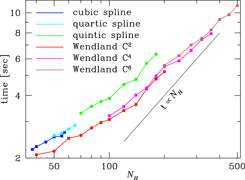
Figure 12: Wall-clock timings for an (average) single SPH time step (using four processors) for $N=2^{20}$ particles as function of neighbour number $N_{\!H}$ for the kernels of Table 1.

5.2 Are there more useful kernel functions?

Neither the B-splines nor the Wendland functions have been designed with SPH or the task of density estimation in mind, but derive from interpolation of function values $y_{i}$ for given points $\boldsymbol{x}_{i}$.

The B-splines were constructed to exactly interpolate polynomials on a regular 1D grid. However, this for itself is not a desirable property in the context of SPH, in particular for 2D and 3D.

The Wendland functions were designed for interpolation of scattered multi-dimensional data, viz

$$\textstyle s(\boldsymbol{x})=\sum_{j}\alpha_{\!j}\,w(|\boldsymbol{x}-\boldsymbol{x}_{\!j}|).$$

The coefficients $\alpha_{\!j}$ are determined by matching the interpolant $s(\boldsymbol{x})$ to the function values, resulting in the linear equations

$$\textstyle y_{i}=\sum_{j}\alpha_{\!j}\,w(|\boldsymbol{x}_{i}-\boldsymbol{x}_{\!j}|),\quad i=1\dots n.$$

If the matrix $\mathsf{W}_{\!i\!j}=w(|\boldsymbol{x}_{i}-\boldsymbol{x}_{\!j}|)$ is positive definite for any choice of $n$ points $\boldsymbol{x}_{i}$, then this equation can always be solved. Moreover, if the function $w(r)$ has compact support, then $\boldsymbol{\mathsf{W}}$ is sparse, which greatly reduces the complexity of the problem. The Wendland functions were designed to fit this bill. As a side effect they have non-negative Fourier transform (according to Bochner, 1933), which together with their compact support, smoothness, and computational simplicity makes them ideal for SPH with large $N_{\!H}$.

So far, the Wendland functions are the only kernels which are stable against pairing for all $N_{\!H}$ and satisfy all other desirable properties from the list on page 2.2.

5.3 What is the SPH resolution scale?

In smooth flows, i.e. in the absence of particle disorder, the only error of the SPH estimates is the bias induced by the smoothing operation. For example, assuming a smooth density field

$$\hat{\rho}_{i}\approx\rho(\boldsymbol{x}_{i})+\tfrac{1}{2}\sigma^{2}\,\boldsymbol{\nabla}^{2}\!\rho(\boldsymbol{x}_{i})+\mathcal{O}(h^{4})$$ (34)

(e.g. Monaghan, 1985; Silverman, 1986) with $\sigma$ defined in equation (8). Since $\sigma$ also sets the resolution of sound waves (§3.1.3), our definition (10), $h=2\sigma$, of the SPH resolution scale is appropriate for smooth flows. The result (34) is the basis for the traditional claim of $\mathcal{O}(h^{2})$ convergence for smooth flows. True flow discontinuities are smeared out over a length scale comparable to $h$ (though we have not made a detailed investigation of this).

In practice, however, particle disorder affects the performance and, as our test simulations demonstrated, the actual resolution of SPH can be much worse than the smooth-flow limit suggests.

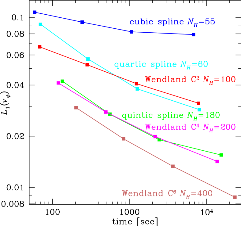
Figure 13: As Fig. 10, except that the $x$-axis shows the computational costs.

5.4 Are large neighbour numbers sensible?

There is no consensus about the best neighbour number in SPH: traditionally the cubic spline kernel is used with $N_{\!H}\approx 42$, while Price (2012) favours $N_{\!H}=57$ (at or even beyond the pairing-instability limit) and Read et al. (2010) use their HOCT4 kernel with even $N_{\!H}=442$ (corresponding to a $1.7$ times larger $h$). From a pragmatic point of view, the number $N$ of particles, the neighbour number $N_{\!H}$, and the smoothing kernel (and between them the numerical resolution) are numerical parameters which can be chosen to optimise the efficiency of the simulation. The critical question therefore is:

Which combination of $N$ and $N_{\!H}$ (and kernel) most efficiently models a given problem at a desired fidelity?

Clearly, this will depend on the problem at hand as well as the desired fidelity. However, if the problem contains any chaotic or turbulent flows, as is common in star- and galaxy formation, then the situation exemplified in the Gresho-Chan vortex test of §4.2 is not atypical and large $N_{\!H}$ may be required for sufficient accuracy.

But are high neighbour numbers affordable? In Fig. 12, we plot the computational cost versus $N_{\!H}$ for different kernels. At $N_{\!H}\lesssim 400$ the costs rise sub-linearly with $N_{\!H}$ (because at low $N_{\!H}$ SPH is data- rather than computation-dominated) and high $N_{\!H}$ are well affordable. In the case of the vortex test, they are absolutely necessary as Fig. 13 demonstrates: for a given numerical accuracy, our highest $N_{\!H}$ makes optimal use of the computational resources (in our code memory usage does not significantly depend on $N_{\!H}$, so CPU time is the only relevant resource).

6 Summary

Particle disorder is unavoidable in strong shear (ubiquitous in astrophysical flows) and causes random errors of the SPH force estimator. The good news is that particle disorder is less severe than Poissonian shot noise and the resulting force errors (which are dominated by the ‘E₀’ term of Read et al., 2010) are not catastrophic. The bad news, however, is that these errors are still significant enough to spoil the convergence of SPH.

In this study we investigated the option to reduce the ‘E₀ errors’ by increasing the neighbour number in conjunction with a change of the smoothing kernel. Switching from the cubic to the quintic spline at fixed resolution $h$ increases the neighbour number $N_{\!H}$ only by a factor 1.74, hardly enough to combat ‘E₀ errors’. For a significant reduction of the these errors one has to trade resolution and significantly increase $N_{\!H}$ beyond conventional values.

The main obstacle with this approach is the pairing instability, which occurs for large $N_{\!H}$ with the traditional SPH smoothing kernels. In §3 and appendix A, we have performed (it appears for the first time) a complete linear stability analysis for conservative SPH in any number of spatial dimensions. This analysis shows that SPH smoothing kernels whose Fourier transform is negative for some wave vector $\boldsymbol{k}$ will inevitably trigger the SPH pairing instability at sufficiently large neighbour number $N_{\!H}$. Such kernels therefore require $N_{\!H}$ to not exceed a certain threshold in order to avoid the pairing instability (not to be confused with the tensile instability, which has the same symptoms but is caused by a negative effective pressure independent of the kernel properties).

Intuitively, the pairing instability can be understood in terms of the SPH density estimator: if a paired particle distribution obtains a lower average estimated density, its estimated total thermal energy $\hat{U}$ is smaller and hence favourable. Otherwise, the smallest $\hat{U}$ occurs for a regular distribution, driving the automatic maintenance of particle order, a fundamental ingredient of SPH.

The Wendland (1995) functions, presented in §2.2.3, have been constructed, albeit for different reasons, to possess a non-negative Fourier transform, and be of compact support with simple functional form. The first property and the findings from our tests in §4.1 demonstrate the remarkable fact that these kernels are stable against pairing for all neighbour numbers (this disproves the long-cultivated myth that the pairing instability was caused by a maximum in the kernel gradient). Our 3D test simulations show that the cubic, quartic, and quintic spline kernels become unstable to pairing for $N_{\!H}>55$, 67, and 190, respectively (see Fig. 8), but operating close to these thresholds cannot be recommended.

A drawback of the Wendland kernels is a comparably large density error at low $N_{\!H}$. As we argue in §5.1.1, this error is directly related to the stability against pairing. However, in §2.5 we present a simple method to correct for this error without affecting the stability properties and without any other adverse effects.

We conclude, therefore, that the Wendland functions are ideal candidates for SPH smoothing kernels, in particular when large $N_{\!H}$ are desired, since they are computationally superior to the high-order B-splines. All other alternative kernels proposed in the literature are computationally more demanding and are either centrally spiked, like the HOCT4 kernel of Read et al. (2010), or susceptible to pairing like the B-splines (e.g. Cabezón et al., 2008).

Our tests of Section 4 show that simulations of both strong shear flows and shocks benefit from large $N_{\!H}$. These tests suggest that for $N_{\!H}\sim 200$ and 400, respectively, the Wendland $C^{4}$ and $C^{6}$ kernels are most suitable. Compared to $N_{\!H}=55$ with the standard cubic spline kernel, these kernel-$N_{\!H}$ combinations have lower resolution ($h$ increased by factors 1.27 and 1.44, respectively), but obtain much better convergence in our tests.

For small neighbour numbers, however, these tests and our linear stability analysis unexpectedly show that the quartic B-spline kernel with $N_{\!H}=60$ is clearly superior to the traditional cubic spline and can compete with the Wendland $C^{2}$ kernel with $N_{\!H}=100$. The reason for this astonishing performance of the quartic spline is unclear, perhaps the fact that near $\boldsymbol{x}=0$ this spline is more than three times continuously differentiable plays a role.

We note that, while the higher-degree Wendland functions are new to SPH, the Wendland $C^{2}$ kernel has already been used (Monaghan 2011, for example, employs it for 2D simulations). However, while its immunity to the pairing instability has been noted (e.g. Robinson, 2009), we are not aware of any explanation (previous to ours) nor of any other systematic investigation of the suitability of the Wendland functions for SPH.

Appendix A Linear Stability Analysis

We start from an equilibrium with particles of equal mass $m$ on a regular grid and impose a plane-wave perturbation to the unperturbed positions $\bar{\boldsymbol{x}}_{i}$ (a bar denotes a quantity obtained for the unperturbed equilibrium):

$$\boldsymbol{x}_{i}=\bar{\boldsymbol{x}}_{i}+\boldsymbol{\xi}_{i},\qquad\boldsymbol{\xi}_{i}=\boldsymbol{a}\,\Phi_{i}(\boldsymbol{x},t),\qquad\Phi_{i}(\boldsymbol{x},t)=\mathrm{e}^{i(\boldsymbol{k}{\cdot}\bar{\boldsymbol{x}}_{i}-\omega t)}.$$ (35)

as in equation (20). We derive the dispersion relation $\omega(\boldsymbol{k},\boldsymbol{a})$ by equating the SPH force imposed by the perturbation (to linear order) to its acceleration

$$\ddot{\boldsymbol{\xi}}_{i}=-\boldsymbol{a}\,\omega^{2}\,\Phi_{i}(\boldsymbol{x},t).$$ (36)

To obtain the perturbed SPH forces to linear order, we develop the internal energy of the system, and hence the SPH density estimate, to second order in $\boldsymbol{\xi}_{i}$. If $\hat{\rho}_{i}=\bar{\rho}+\rho_{i1}+\rho_{i2}$ with $\rho_{i1}$ and $\rho_{i2}$ the first and second-order density corrections, respectively, then

$$\ddot{\boldsymbol{\xi}}_{i}=-\frac{1}{m}\frac{\partial\mathcal{L}}{\partial\boldsymbol{\xi}_{i}}=-\frac{\bar{P}}{\bar{\rho}}\sum_{k}\frac{1}{\bar{\rho}}\frac{\partial\rho_{k2}}{\partial\boldsymbol{\xi}_{i}}-\left(\bar{c}^{2}-\frac{2\bar{P}}{\bar{\rho}}\right)\frac{1}{2\bar{\rho}^{2}}\sum_{k}\frac{\partial\rho_{k1}^{2}}{\partial\boldsymbol{\xi}_{i}}.$$ (37)

A.1 Fixed $h$

Let us first consider the simple case of constant $h=\bar{h}$ which remains unchanged during the perturbation. Then,

$$\textstyle\rho_{in}=\varrho_{in}/n!\quad\text{with}\quad\varrho_{in}=\sum_{j}m\,(\boldsymbol{\xi}_{i\!j}{\cdot}\boldsymbol{\nabla})^{n}W(\bar{\boldsymbol{x}}_{i\!j},\bar{h}).$$ (38)

Inserting

$$\boldsymbol{\xi}_{i\!j}=\boldsymbol{\xi}_{i}-\boldsymbol{\xi}_{\!j}=\boldsymbol{a}\big{(}1-\mathrm{e}^{-i\boldsymbol{k}{\cdot}\bar{\boldsymbol{x}}_{i\!j}}\big{)}\,\Phi_{i}$$ (39)

into (38) gives

$$\textstyle\varrho_{i1}=\Phi_{i}\,\sum_{j}m\,\big{(}1-\mathrm{e}^{-i\boldsymbol{k}{\cdot}\bar{\boldsymbol{x}}_{i\!j}}\big{)}\,\boldsymbol{a}{\cdot}\boldsymbol{\nabla}W(\bar{\boldsymbol{x}}_{i\!j},\bar{h})=i\,\Phi_{i}\,\boldsymbol{a}{\cdot}\boldsymbol{t},$$ (40)

where (assuming a symmetric particle distribution)

$$\textstyle\boldsymbol{t}(\boldsymbol{k})=\sum_{j}m\sin\boldsymbol{k}{\cdot}\bar{\boldsymbol{x}}_{\!j}\,\boldsymbol{\nabla}W(\bar{\boldsymbol{x}}_{\!j},\bar{h}).$$ (41)

We can then derive

$$\textstyle\sum_{k}\varrho_{k1}\,\partial\varrho_{k1}/\partial\boldsymbol{\xi}_{i} = \textstyle\sum_{k}\varrho_{k1}\,\sum_{j}m\,\boldsymbol{\nabla}W(\bar{\boldsymbol{x}}_{k\!j},\bar{h})\big{(}\delta_{ik}-\delta_{i\!j}\big{)}$$ (42)

$$= \textstyle\sum_{j}m\,(\varrho_{i1}+\varrho_{j1})\boldsymbol{\nabla}W(\bar{\boldsymbol{x}}_{i\!j},\bar{h})$$

$$= \textstyle i\,\Phi_{i}\,\boldsymbol{a}{\cdot}\boldsymbol{t}\sum_{j}m\,\big{(}1+\mathrm{e}^{-i\boldsymbol{k}{\cdot}\bar{\boldsymbol{x}}_{i\!j}}\big{)}\,\boldsymbol{\nabla}W(\bar{\boldsymbol{x}}_{i\!j},\bar{h})$$

$$= \Phi_{i}\,\boldsymbol{a}{\cdot}\boldsymbol{t}\,\boldsymbol{t},$$

$$\textstyle\tfrac{1}{2}\sum_{k}\partial\varrho_{k2}/\partial\boldsymbol{\xi}_{i} = \textstyle\sum_{k\!j}m\,(\boldsymbol{\xi}_{k\!j}{\cdot}\boldsymbol{\nabla})\boldsymbol{\nabla}W(\bar{\boldsymbol{x}}_{k\!j},\bar{h})\big{(}\delta_{ik}-\delta_{i\!j}\big{)}$$ (43)

$$= \textstyle 2\sum_{j}m\,(\boldsymbol{\xi}_{i\!j}{\cdot}\boldsymbol{\nabla})\boldsymbol{\nabla}W(\bar{\boldsymbol{x}}_{i\!j},\bar{h})$$

$$= \textstyle 2\Phi_{i}\,\sum_{j}m\,\big{(}1-\mathrm{e}^{-i\boldsymbol{k}{\cdot}\bar{\boldsymbol{x}}_{i\!j}}\big{)}\,\boldsymbol{a}{\cdot}\boldsymbol{\nabla}\boldsymbol{\nabla}W(\bar{\boldsymbol{x}}_{k\!j},\bar{h})$$

$$= 2\Phi_{i}\,\boldsymbol{a}{\cdot}\boldsymbol{\mathsf{T}}$$

with

$$\textstyle\boldsymbol{\mathsf{T}}(\boldsymbol{k})=\sum_{j}m\,\big{(}1-\cos\boldsymbol{k}{\cdot}\bar{\boldsymbol{x}}_{\!j}\big{)}\,\boldsymbol{\nabla}^{(2)}W(\bar{\boldsymbol{x}}_{\!j},\bar{h}).$$ (44)

Inserting these results into (37), we get

$$\ddot{\boldsymbol{\xi}}_{i} = -\frac{2\bar{P}}{\bar{\rho}}\frac{\boldsymbol{a}{\cdot}\boldsymbol{\mathsf{T}}}{\bar{\rho}}\Phi_{i}-\left(\bar{c}^{2}-\frac{2\bar{P}}{\bar{\rho}}\right)\frac{\boldsymbol{a}{\cdot}\boldsymbol{t}\,\boldsymbol{t}}{\bar{\rho}^{2}}\Phi_{i}.$$ (45)

A.2 Adaptive smoothing

If the $h_{i}$ are adapted such that $M_{i}\equiv h_{i}^{\nu}\hat{\rho}_{i}$ remains a global constant $\bar{M}$, the estimated density is simply $\hat{\rho}_{i}=\bar{M}h_{i}^{-\nu}$. We start by expanding $M_{i}$ to second order in both $\boldsymbol{a}$ and $\eta_{i}\equiv\ln(h_{i}/\bar{h})$. Using a prime to denote differentiation w.r.t. $\ln\bar{h}$, we have

$$M_{i} = M_{h}+\bar{h}^{\nu}\!\varrho_{i1}+\eta\big{(}\bar{h}^{\nu}\bar{\rho}\big{)}^{\prime}+\tfrac{1}{2}\bar{h}^{\nu}\!\varrho_{i2}+\eta\big{(}\bar{h}^{\nu}\!\varrho_{i1}\big{)}^{\prime}+\tfrac{1}{2}\eta^{2}\big{(}\bar{h}^{\nu}\bar{\rho}\big{)}^{\prime\prime}$$ (46a)

$$= M_{h}+\bar{h}^{\nu}\left[\varrho_{i1}+\eta\nu\bar{\rho}\bar{\Omega}+\tfrac{1}{2}\varrho_{i2}+\eta\varrho_{i1}^{\prime}+\eta\nu\varrho_{i1}+\tfrac{1}{2}\eta^{2}\nu^{2}\bar{\rho}\bar{\Pi}\right]$$ (46b)

with $\bar{\Omega}\simeq 1$ as defined in equation (4) and

$$\bar{\Pi}=\frac{1}{\nu^{2}\bar{h}^{\nu}\bar{\rho}}\,\frac{\partial^{2}(\bar{h}^{\nu}\bar{\rho})}{\partial(\ln\bar{h})^{2}}=\frac{1}{\nu\bar{h}^{\nu}\bar{\rho}}\,\frac{\partial(\bar{h}^{\nu}\bar{\rho}\bar{\Omega})}{\partial\ln\bar{h}}\simeq 1.$$ (47)

By demanding $M_{i}=\bar{M}$, we obtain for the first- and second-order contributions to $\eta_{i}$

$$-\nu\bar{\rho}\eta_{i1} = \frac{\varrho_{i1}}{\bar{\Omega}}$$ (48a)

$$-\nu\bar{\rho}\eta_{i2} = \frac{\varrho_{i2}}{2\bar{\Omega}}+\frac{\eta_{i1}\varrho_{i1}^{\prime}}{\bar{\Omega}}+\frac{\nu\eta_{i1}\varrho_{i1}}{\bar{\Omega}}+\frac{\nu^{2}\eta_{i1}^{2}\bar{\rho}\bar{\Pi}}{2\bar{\Omega}}$$ (48b)

$$= \frac{\varrho_{i2}}{2\bar{\Omega}}-\frac{(\varrho_{i1}^{2})^{\prime}}{2\nu\bar{\rho}\bar{\Omega}^{2}}-\frac{\varrho_{i1}^{2}}{\bar{\rho}\bar{\Omega}^{2}}+\frac{\varrho_{i1}^{2}\bar{\Pi}}{2\bar{\rho}\bar{\Omega}^{3}}.$$ (48c)

From these expressions and $\hat{\rho}_{i}=\bar{\rho}\mathrm{e}^{-\nu\eta_{i}}$ we obtain the first and second order density corrections

$$\rho_{i1} =-\nu\bar{\rho}\eta_{i1}\phantom{\;\,+\tfrac{1}{2}\nu^{2}\bar{\rho}\eta_{i1}^{2}}= \frac{\varrho_{i1}}{\bar{\Omega}},$$ (49a)

$$\rho_{i2} =-\nu\bar{\rho}\eta_{i2}+\tfrac{1}{2}\nu^{2}\bar{\rho}\eta_{i1}^{2}= \frac{\varrho_{i2}}{2\bar{\Omega}}-\frac{(\varrho_{i1}^{2})^{\prime}}{2\nu\bar{\rho}\bar{\Omega}^{2}}+\frac{\varrho_{i1}^{2}(\bar{\Pi}-\bar{\Omega})}{2\bar{\rho}\bar{\Omega}^{3}}.$$ (49b)

Inserting these expressions into equation (37) we find with relations (42) and (43)

$$\ddot{\boldsymbol{\xi}}_{i} = -\frac{\bar{P}}{\bar{\rho}}\left(2\frac{\boldsymbol{a}{\cdot}\boldsymbol{\mathsf{T}}}{\bar{\rho}\bar{\Omega}}+\bar{\Xi}\frac{\boldsymbol{a}{\cdot}\boldsymbol{t}\,\boldsymbol{t}}{\bar{\rho}^{2}\bar{\Omega}^{2}}-\frac{1}{\nu\bar{\rho}^{2}\bar{\Omega}^{2}}\frac{\partial(\boldsymbol{a}{\cdot}\boldsymbol{t}\,\boldsymbol{t})}{\partial\ln\bar{h}}\right)\Phi_{i}$$ (50)

$$-\left(\bar{c}^{2}-\frac{2\bar{P}}{\bar{\rho}}\right)\frac{\boldsymbol{a}{\cdot}\boldsymbol{t}\,\boldsymbol{t}}{\bar{\rho}^{2}\bar{\Omega}^{2}}\,\Phi_{i}.$$

where

$$\bar{\Xi}\equiv\frac{\bar{\Pi}}{\bar{\Omega}}-1=\frac{1}{\nu}\frac{\partial\ln(\bar{\rho}\bar{\Omega})}{\partial\ln\bar{h}}\simeq 0.$$ (51)

A.3 The limit $\boldsymbol{k}\to 0$

From equation (5) $h^{\nu}\boldsymbol{x}{\cdot}\boldsymbol{\nabla}W(\boldsymbol{x},h)=-\partial(h^{\nu}W)/\partial\ln h$, such that

$$-\nu\,\hat{\rho}_{i}\Omega_{i} = \textstyle\sum_{j}m_{j}\boldsymbol{x}_{i\!j}{\cdot}\boldsymbol{\nabla}W(\boldsymbol{x}_{i\!j},h_{i}),$$ (52a)

$$\nu^{2}\hat{\rho}_{i}\Pi_{i} = \textstyle\sum_{j}m_{j}(\boldsymbol{x}_{i\!j}{\cdot}\boldsymbol{\nabla})^{2}W(\boldsymbol{x}_{i\!j},h_{i}).$$ (52b)

Assuming local spatial isotropy we then get in the limit $\boldsymbol{k}\to 0$

$$\boldsymbol{t} \to -\bar{\Omega}\bar{\rho}\,\boldsymbol{k},$$ (53a)

$$\boldsymbol{t}^{\prime} \to -\nu(\bar{\Pi}-\bar{\Omega})\bar{\rho}\,\boldsymbol{k},$$ (53b)

$$\boldsymbol{\mathsf{T}} \to \frac{(2\bar{\Omega}+\nu\bar{\Pi})\bar{\rho}}{2+\nu}\boldsymbol{k}^{(2)}+\frac{\nu(\bar{\Pi}-\bar{\Omega})\bar{\rho}}{2(\nu+2)}|\boldsymbol{k}|^{2}\,\boldsymbol{\mathsf{I}}.$$ (53c)

Inserting these into (50) gives

$$\ddot{\boldsymbol{\xi}}=-\bar{c}^{2}\boldsymbol{a}{\cdot}\boldsymbol{k}\,\boldsymbol{k}\,\Phi_{i}-\frac{\bar{P}}{\bar{\rho}}\bar{\Xi}\left[\bigg{(}\!\frac{2\nu}{2+\nu}-1\!\bigg{)}\,\boldsymbol{a}{\cdot}\boldsymbol{k}\,\boldsymbol{k}+\frac{\nu\boldsymbol{k}^{2}\boldsymbol{a}}{\nu+2}\right]\Phi_{i}.$$ (54)

References

- Abel (2011) Abel T., 2011, MNRAS, 413, 271
- Bochner (1933) Bochner S., 1933, Math. Ann., 108, 378
- Cabezón et al. (2008) Cabezón R. M., García-Senz D., Relaño A., 2008, J. Comp. Phys., 227, 8523
- Cullen & Dehnen (2010) Cullen L., Dehnen W., 2010, MNRAS, 408, 669
- Fulk & Quinn (1996) Fulk D. A., Quinn D. W., 1996, J. Comp. Phys., 126, 165
- Gingold & Monaghan (1977) Gingold R. A., Monaghan J. J., 1977, MNRAS, 181, 375
- Gray et al. (2001) Gray J. P., Monaghan J. J., Swift R. P., 2001, Comp. Meth. Appl. Mech. Eng., 190, 6641
- Gresho & Chan (1990) Gresho P. M., Chan S. T., 1990, Int. J. Num. Meth. Fluids, 11, 621
- Hall (1927) Hall P., 1927, Biometrika, 19, 240
- Herant (1994) Herant M., 1994, Mem. Soc. Astron. Italiana, 65, 1013
- Heß & Springel (2010) Heß S., Springel V., 2010, MNRAS, 406, 2289
- Irwin (1927) Irwin J. O., 1927, Biometrika, 19, 225
- Liska & Wendroff (2003) Liska R., Wendroff B., 2003, SIAM J. Sci. Comp., 25, 995
- Lucy (1977) Lucy L. B., 1977, AJ, 82, 1013
- Monaghan (1985) Monaghan J. J., 1985, J. Comp. Phys., 60, 253
- Monaghan (2000) Monaghan J. J., 2000, J. Comp. Phys., 159, 290
- Monaghan (2002) Monaghan J. J., 2002, MNRAS, 335, 843
- Monaghan (2005) Monaghan J. J., 2005, Reports of Progress in Physics, 68, 1703
- Monaghan (2011) Monaghan J. J., 2011, European J. Mech. B Fluids, 30, 360
- Monaghan (2012) Monaghan J. J., 2012, Ann. Rev. Fluid Mech., 44, 323
- Monaghan & Lattanzio (1985) Monaghan J. J., Lattanzio J. C., 1985, A&A, 149, 135
- Monaghan & Price (2001) Monaghan J. J., Price D. J., 2001, MNRAS, 328, 381
- Morris (1996) Morris J. P., 1996, Pub. Astr. Soc. Aust., 13, 97
- Nelson & Papaloizou (1994) Nelson R. P., Papaloizou J. C. B., 1994, MNRAS, 270, 1
- Phillips & Monaghan (1985) Phillips G. J., Monaghan J. J., 1985, MNRAS, 216, 883
- Price (2012) Price D. J., 2012, J. Comp. Phys., 231, 759
- Rasio (2000) Rasio F. A., 2000, Prog. Theo. Phys. Supp., 138, 609
- Read & Hayfield (2012) Read J. I., Hayfield T., 2012, MNRAS, in press
- Read et al. (2010) Read J. I., Hayfield T., Agertz O., 2010, MNRAS, 405, 1513
- Robinson (2009) Robinson M. J., 2009, PhD thesis, Monash University, Australia
- Rosswog (2009) Rosswog S., 2009, New Astronomy Reviews, 53, 78
- Schoenberg (1946) Schoenberg I. J., 1946, Q. Appl. Math., 4, 45
- Schüßler & Schmitt (1981) Schüßler I., Schmitt D., 1981, A&A, 97, 373
- Silverman (1986) Silverman B. W., 1986, Density estimation for statistics and data analysis. London, Chapman & Hall
- Sod (1978) Sod G. A., 1978, J. Comp. Phys., 27, 1
- Springel (2010) Springel V., 2010, ARA&A, 48, 391