The nonequilibrium discrete nonlinear Schrödinger equation

Abstract

We study nonequilibrium steady states of the one-dimensional discrete nonlinear Schrödinger equation. This system can be regarded as a minimal model for stationary transport of bosonic particles like photons in layered media or cold atoms in deep optical traps. Due to the presence of two conserved quantities, energy and norm (or number of particles), the model displays coupled transport in the sense of linear irreversible thermodynamics. Monte Carlo thermostats are implemented to impose a given temperature and chemical potential at the chain ends. As a result, we find that the Onsager coefficients are finite in the thermodynamic limit, i.e. transport is normal. Depending on the position in the parameter space, the “Seebeck coefficient” may be either positive or negative. For large differences between the thermostat parameters, density and temperature profiles may display an unusual nonmonotonic shape. This is due to the strong dependence of the Onsager coefficients on the state variables.

I Introduction

The Discrete Nonlinear Schrödinger (DNLS) equation Eilbeck et al. (1985); Kevrekidis (2009) has important applications in many domains of physics. As it is well known, such equation arises in several different problems. A classical example is electronic transport in biomolecules Scott (2003). In the context of optics or acoustics it describes the propagation of nonlinear waves in a layered photonic or phononic system. Indeed, in a suitable limit, the dynamics of high-frequency Bloch waves is described by a DNLS equation for their envelope (see Refs. Kosevich and Mamalui (2002); Tsironis and Hennig (1999) for details). On the other hand, in the realm of the physics of cold atomic gases, the equation is an approximate semiclassical description of bosons trapped in periodic optical lattices (see e.g. Ref. Franzosi et al. (2011) and references therein for a recent survey). Many other physical problems have been recently addressed having the DNLS equation as a basic reference model, like the effect of nonlinearity on Anderson localization Kopidakis et al. (2008); Pikovsky and Shepelyansky (2008) and the violation of reciprocity in wave scattering Lepri and Casati (2011) just to mention a few recent examples.

While a vast literature has been devoted to localization problems, much less is known about finite-temperature properties. The first analysis of the equilibrium statistical mechanics of DNLS systems has been performed in Ref. Rasmussen et al. (2000a), while the relaxation of localized modes (discrete breathers) in the presence of phonon baths has been discussed in Rasmussen et al. (2000b); Rumpf (2004). Several results can be translated to other types of nonlinear lattices, where a DNLS-like equation represents an approximation of the lattice dynamics Johansson (2006).

An even less explored field is that of nonequilibrium properties of the DNLS equation Eisner and Turkington (2006). In particular, the case of an open system that exchanges energy with external reservoirs has not been treated so far. The presence of two conserved quantitities naturally requires to argue about coupled transport, in the sense of ordinary linear irreversible thermodynamics. Despite the very many studies of heat conduction in oscillator chains Lepri et al. (2003); Dhar (2008), works on coupled transport are scarce Gillan and Holloway (1985); Mejia-Monasterio et al. (2001); Larralde et al. (2003). Interest in this field has been revived by recent works on thermoelectric phenomena Casati et al. (2008, 2009) in the hope of identifying dynamical mechanisms that could enhance the efficiency of thermoelectric energy conversion Horvat et al. (2009); Saito et al. (2010).

In order to investigate transport properties, we need to introduce the interaction of the system with external reservoirs that are capable to exchange energy and/or norm. For models like DNLS this is much less straightforward than for standard oscillator chains, where e.g. Langevin thermostats are a typical choice Lepri et al. (2003); Dhar (2008). Here we propose and test a very simple Monte Carlo scheme which is easy to implement and suitable for the model at hand. Another important difference between the DNLS and standard oscillator chains (like the Fermi-Pasta-Ulam or Klein-Gordon models) is that its Hamiltonian is not the sum of kinetic and potential energies. Thus, it is necessary to introduce suitable operative definitions of kinetic temperature $T$ and chemical potential $\mu$, to measure such quantities in actual simulations. In the following, we make use of a recent definition of the microcanonical temperature Franzosi (2011) and extend it for the estimate of the chemical potential.

By imposing small $T$ and $\mu$ jumps across the chain, we can determine the Onsager coefficients, which turn out to be finite in the thermodynamic limit, i.e. both energy and mass conductions are normal processes. From the Onsager coefficients we can thereby determine the “Seebeck coefficient” $S$ note1 which we find to be either positive or negative, depending on the thermodynamic parameters (i.e., mass and energy density). For larger temperature or chemical-potential differences, although one can still invoke the linear response theory, some surprising phenomena emerge. One example is the “anomalous heating” that can be observed when the chain is attached to two thermostats operating at the same temperature: along the chain, $T$ reaches values that are even three times larger than that imposed on the boundaries. This phenomenon can be observed only in the case of coupled transport, since it is due to the variable weight of the non-diagonal terms of the Onsager matrix. It is apparent in the DNLS, because of the strong variability of the Onsager coefficients.

The paper is organized as follows. In Sec. II we introduce the model and describe the heat baths. In Sec. III, we define the relevant thermodynamic observables and the formalism (e.g., the Onsager coefficients) necessary to characterize nonequilibrium steady states. Sec. IV is devoted to a discussion of the stead states, both in the case of small and large $T$, $\mu$ differences. In Sec. V we provide a pictorial representation of the general transport properties, by reconstructing the zero-flux curves. Finally, the last section is devoted to the conclusions and to a brief summary of the open problems.

II Setup

In one dimension, the DNLS Hamiltonian writes

$$H=\frac{1}{4}\sum_{i=1}^{N}\left(p_{i}^{2}+q_{i}^{2}\right)^{2}+\sum_{i=1}^{N-1}\left(p_{i}p_{i+1}+q_{i}q_{i+1}\right)\quad,$$ (1)

where the sum runs over the $N$ sites of the chain. The sign of quartic term is positive, as we refer to a repulsive-atom BEC, while the sign of the hopping term is irrelevant, due to the symmetry associated with the canonical (gauge) transformation $z_{n}\to z_{n}e^{i\pi n}$ (where $z_{n}\equiv(p_{n}+\imath q_{n})/\sqrt{2}$ denotes the amplitude of the wave function). The equations of motion are

$$i\dot{z}_{n}=-z_{n+1}-z_{n-1}-2|z_{n}|^{2}z_{n}$$ (2)

with $n=1,\cdots,N$, and fixed boundary conditions ($z_{0}=z_{N+1}=0$). The model has two conserved quantities, the energy and the total norm (or total number of particles)

$$A=\sum_{i=1}^{N}(p_{i}^{2}+q_{i}^{2})\quad.$$ (3)

As a consequence, the equilibrium phase-diagram is two-dimensional, as it involves the energy density $h=H/N$ and the particle density $a=A/N$. The first reconstruction of the diagram was carried out in Ref. Rasmussen et al. (2000a) within the grand-canonical ensemble with the help of transfer integral techniques. It is schematically described in Fig. 1: the lower dashed line corresponds to the ground state ($T=0$) upon varying the particle density; the upper dashed line corresponds to infinite temperature. The nonequilibrium studies described in this paper correspond to the region in between such two curves.

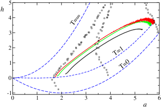
Figure 1: (Color online) Parametric plots of the local norm and energies $[a(y)$, $h(y)]$ for $T_{L}=T_{R}=1$, $\mu_{L}=0$, $\mu_{R}=2$ and increasing chain lengths $N=200,800,3200$ (solid lines, bottom to top). The three (blue) dashed lines are the isothermal $T=0$, $T=1$ and $T=\infty$ respectively. Lines at constant chemical potential (open symbols) $\mu=0$, $\mu=1$ and $\mu=2$ (left to right respectively) are obtained by equilibrium simulations.

We aim at characterizing the steady states of the chain when put in contact (on the left and right boundaries) with two thermostats at temperature $T_{L}$ and $T_{R}$ and chemical potentials $\mu_{L}$ and $\mu_{R}$, respectively. The implementaton of the interactions with a heat bath is often based on heuristics. In particle models, the simpler schemes consist in either adding a Langevin noise, or in assuming random collisions with an equilibrium gas Lepri et al. (2003); Dhar (2008). For the DNLS this is less straightforward: adding white noise and a linear dissipation drives the system to infinite temperature, i.e. to a state in which relative phases are uncorrelated.

In the absence of a first-principle definition of heat bath, we consider two phenomenological Monte-Carlo heat baths. The general scheme of this kind of heat bath involves a stochastic dynamics which perturbs the canonical variables $p_{1}\to p_{1}+\delta p_{1}$ and $q_{1}\to q_{1}+\delta q_{1}$ note2 at random times, chosen according to a uniform distribution in the interval $[t_{min},t_{max}]$. The perturbations $\delta p$ and $\delta q$ are independent random variables uniformly distributed in the interval $[-R,R]$. Moves are accepted according to the standard Metropolis algorithm, evaluating the cost function $\exp{\{-T_{L}^{-1}(\Delta H-\mu_{L}\Delta A)\}}$ with $T_{L}$ and $\mu_{L}$ being the temperature and the chemical potential of the heat bath. This kind of thermostat exchanges both energy and particles. In some cases, however, we need to study the chain behavior in the absence of one of the two fluxes (energy and norm). A simple way to study these setups is to modify the perturbation rule of the thermostat, requiring the exact conservation of the corresponding local density (energy density or norm density). We have thus the following two schemes:

Norm conserving thermostat- The perturbation acts only on the phase $\phi_{1}$ of the complex variable $z_{1}$. More precisely we impose $\phi_{1}\to\phi_{1}+\delta\phi_{1}\ \ mod(2\pi)$, where $\delta\phi$ is a random variable, uniformly distributed in the interval $[0,2\pi]$. This dynamics conserves exactly the local amplitude $|z_{1}|^{2}$ and therefore the total norm $A$.

Energy conserving thermostat- In this case, it is necessary to go through two steps to conserve the energy

$$e_{1}=|z_{1}|^{4}+2|z_{1}||z_{2}|\cos{(\phi_{1}-\phi_{2})}\quad.$$ (4)

First, the amplitude $|z_{1}|$ is randomly perturbed. As a result, both the local amplitude and the local energy change. Then, by inverting, Eq. (4), a value of $\phi_{1}$ that restores the initial energy is seeked. If no such solution exists, we go back to the first step and choose a new perturbation for $|z_{1}|$.

There is a basic difference between the two types of thermostats. In the general scheme, a steady state is characterized by four parameters $T_{L}$, $T_{R}$, $\mu_{L}$, $\mu_{R}$. On the other hand, for the norm-conserving scheme we only assign $T_{L}$, $T_{R}$ and the norm density $a_{tot}$ of the whole chain. As a consequence, the value of $\mu$ on the boundary is not fixed and must be computed from the simulation. If the steady state is unique, the former thermostating scheme must yield the same results, once the chemical potentials are suitably fixed. A numerical test of this equivalence has been performed, by reconstructing some zero-flux profiles with both thermostats. The curves overlap reasonably well, although some small systematic deviations are present. This is because the norm flux is never exactly zero in the non-conservative case (typically of order $\sim 10^{-4}$ in a chain of 1000 sites). In addition, there are slightly different thermal resistance effects in the two schemes. Besides those discrepancies, we conclude that the proposed schemes work equally well for the generation of nonequilibrium steady states.

III Physical observables

In order to characterize the thermodynamic properties of the DNLS, we extend the approach of Ref. Franzosi (2011) to derive an operative definition not only of the microcanonical temperature but also of the chemical potential. The starting point are the usual definitions $T^{-1}=\partial{\mathcal{S}}/\partial{H}$, and $\mu/T=-\partial{\mathcal{S}}/\partial{A}$, where $\mathcal{S}$ is the thermodynamic entropy. The partial derivatives must be computed taking into account the existence of two conserved quantities (hereafter called $C_{1}$ and $C_{2}$). Thus,

$$\frac{\partial\mathcal{S}}{\partial C_{1}}=\left\langle\frac{W\|\vec{\xi}\|}{\vec{\nabla}C_{1}\cdot\vec{\xi}}\ \vec{\nabla}\cdot\left(\frac{\vec{\xi}}{\|\vec{\xi}\|W}\right)\right\rangle$$ (5)

where $\langle\>\rangle$ stands for the microcanonical average,

$$\vec{\xi} = \frac{\vec{\nabla}C_{1}}{\|\vec{\nabla}C_{1}\|}-\frac{(\vec{\nabla}C_{1}\cdot\vec{\nabla}C_{2})\vec{\nabla}C_{2}}{\|\vec{\nabla}C_{1}\|\|\vec{\nabla}C_{2}\|^{2}}$$ (6)

$$W^{2} = \sum_{\genfrac{}{}{0.0pt}{}{j,k=1}{j<k}}^{2N}\left[\frac{\partial C_{1}}{\partial x_{j}}\frac{\partial C_{2}}{\partial x_{k}}-\frac{\partial C_{1}}{\partial x_{k}}\frac{\partial C_{2}}{\partial x_{j}}\right]^{2}\,,$$

and $x_{2j}=q_{j}$, $x_{2j+1}=p_{j}$. By setting $C_{1}=H$ and $C_{2}=A$, the above formula reduces to the expression for $T$ derived in Franzosi (2011). Moreover, by assuming $C_{1}=A$ and $C_{2}=H$, Eq. (5) defines the chemical potential $\mu$. Notice that both expressions are nonlocal. Nevertheless, we have verified that it is sufficient to compute the expression (5) over as few as 10 sites to obtain, after some time averaging, reliable “local” estimates of both $T$ and $\mu$ note3 .

The expressions for the local energy- and particle-fluxes are derived in the usual way from the continuity equations for norm and energy densities, respectively

$$j_{a}(n)=2\left(p_{n+1}q_{n}-p_{n}q_{n+1}\right)$$ (7)

$$j_{h}(n)=-\left(\dot{p}_{n}p_{n-1}+\dot{q}_{n}q_{n-1}\right)$$ (8)

The approach to the steady state is controlled by verifying that the (time) average fluxes are constant along the chain ($\overline{j_{a}(n)}=j_{a}$ and $\overline{j_{h}(n)}=j_{h}$). Moreover it is also checked that $j_{a}$ and $j_{h}$ are respectively equal to the average energy and norm exchanged per unit time with the reservoirs.

As usual in nonequilibrium molecular dynamics simulations, some tuning of the bath parameters is required to minimize boundary resistance and decrease the statistical errors, as well as the finite-size effects Lepri et al. (2003). For our Monte-Carlo thermostats, we observed that it is necessary to tune the perturbation amplitude $R$. Typically, there is an optimal value of $R$ for which one of the two currents is maximal (keeping the other parameters fixed), but this value may depend on $T$ and $\mu$. Since it would be unpractical to tune the thermostat parameters in each simulation, we decided to fix them in most of the cases. In particular we have chosen $R=0.5$, $t_{min}=10^{-2}$ and $t_{max}=10^{-1}$. Some adjustments have been made only when the fluxes were very small.

In the thermodynamic limit (i.e. for sufficiently long chains), the local forces acting on the system are very weak and one can thereby invoke the linear response theory. This means that forces and fluxes are related by the relations Saito et al. (2010)

$$j_{a} = -L_{aa}\frac{d(\beta\mu)}{dy}+L_{ah}\frac{d\beta}{dy}$$ (9)

$$j_{h} = -L_{ha}\frac{d(\beta\mu)}{dy}+L_{hh}\frac{d\beta}{dy}$$

where we have introduced the continuous variable $y=i/N$, while $\beta$ denotes the inverse temperature $1/T$; $\bf{L}$ is the symmetric, positive definite, $2\times 2$ Onsager matrix. Notice that the first term in the r.h.s. of the above equations is negative, since the thermodynamic forces are $-\beta\mu$ and $\mu$ and that ${\rm det}{\bf L}=L_{aa}L_{hh}-L_{ha}^{2}>0$.

The particle ($\sigma$) and thermal ($\kappa$) conductivity can be expressed expressed in terms of $\bf{L}$,

$$\sigma=\beta L_{aa};\quad\kappa=\beta^{2}\frac{{\rm det}\bf{L}}{L_{aa}}\,.$$ (10)

Analogously, the Seebeck coefficient $S$, which corresponds to (minus) the ratio between the chemical-potential gradient and the temperature gradient (in the absence of a mass flux), writes

$$S=\beta\left(\frac{L_{ha}}{L_{aa}}-\mu\right),$$ (11)

We conclude this Section, by mentioning another important parameter, the figure of merit

$$ZT=\frac{\sigma S^{2}T}{\kappa}=\frac{(L_{ha}-\mu L_{aa})^{2}}{detL};$$

which determines the efficiency $\eta$ for the conversion of a heat current into a particle current as Saito et al. (2010)

$$\eta=\eta_{C}\frac{\sqrt{ZT+1}-1}{\sqrt{ZT+1}+1}.\qquad$$

For large $ZT$, $\eta$ approaches the Carnot limit $\eta_{C}$. Understanding the microscopic mechanisms leading to an increase of $ZT$ is currently an active topic of research Casati et al. (2008).

IV Steady states

IV.1 Local analysis

In a first series of simulations we have studied the nonequilibrium states in the case of small differences between the two thermostats, verifying that transport is normal, i.e. the Onsager coefficients are finite in the thermodynamic limit. This is less obvious than one could have imagined Iubini et al. . In any case, for fixed $\Delta T=T_{R}-T_{L}$ and $\Delta\mu=\mu_{R}-\mu_{L}$, the two fluxes $j_{a}$ and $j_{h}$ are inversely proportional to the system size $N$. At high enough temperatures, the asymptotic scaling sets in already in chains a few hundred sites long (see Fig. 2a). Moreover, if $\Delta T$ $\Delta\mu$ and are small enough, the profiles of $T$ and $\mu$ along the chain are linear as expected.

However, upon decreasing the temperature, the minimal chain length needed to observe a normal transport, becomes very large. As shown in Fig. 2b, for the same range of lattice sizes as in panel a, the currents are almost independent on $N$, as one would expect in the case of ballistic transport. This is because at small temperatures, one can always linearize the equations of motion around the ground state (which depends on the norm density), obtaining a harmonic description and thereby an integrable dynamics.

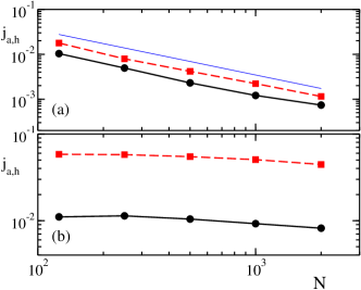
Figure 2: Average energy current (squares) and norm current (dots) versus chain size $N$: (a) High-temperature regime $T_{L}=2$, $T_{R}=4$, $\mu=0$ and (b) Low-temperature regime $T_{L}=0.3$, $T_{R}=0.7$, $\mu=1.5$ The thin (blue) line is the $1/N$ behavior expected for normal transport. Each value is obtained by computing the fluxes on a run of $5\times 10^{6}$ time units.

A plot of the four Onsager coefficients in the $(T,\mu)$ plane is reported in Fig. 3. Within statistical errors, the off-diagonal terms are always positive in the considered range. All coefficients are larger for small $T$ and large $\mu$. This is connected to the scaling behaviour of the linear coefficients in the vicinity of the ground state Iubini et al. .

The resulting coefficient $S$ is plotted in Fig. 4a, where one can see that there are two regions where the Seebeck coefficient is positive, resp. negative, separated by a curve which, according to Eq. (11), is defined by $L_{ha}/L_{aa}=\mu$ (see below). This means that the relative sign of the temperature and chemical-potential gradients is opposite in the two regions (in the presence of a zero norm-flux). This is indeed seen in Fig. 4b where the result of two different simulations are plotted in the two regions.

Finally, since the figure of merit $ZT$ roughly follows $S$, there is only a modest change in the considered parameter ranges. Moreover, for fixed $T$, $ZT$ decreases upon increasing $\mu$. This is qualitatively in agreement with the general expectation that an increasing strength of interaction (increasing $\mu$ means increasing the average norm and thus the nonlinearity) is detrimental for the efficiency.

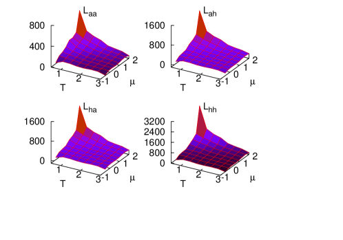
Figure 3: Elements of the Onsager matrix $L$ in the $T,\mu$ plane. for a chain of length $N=500$; $\Delta T=0.1$, $\Delta\mu=0.05$. Each value is obtained by computing the fluxes on a run of $5\times 10^{6}$ time units.

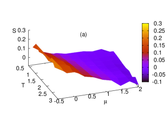
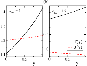
Figure 4: (Color online) (a) Seebeck coefficient $S$ obtained from the data in Fig. 3; (b) Temperature and chemical protential profiles for $T_{L}=1$, $T_{R}=1.5$; simulation with norm-conserving thermostats at two values of the norm density $a_{tot}$ corresponding to values of $S$ with opposite signs.

IV.2 Global analysis

If the temperature- or the chemical-potential difference is no longer small, the temperature and chemical-potential profiles are expected to have a nonlinear shape. This is because, as we have seen in the previous subsection, the Onsager matrix varies with $a$ and $h$ (or, equivalently, with $T$ and $\mu$).

A particularly striking example is reported in Fig. 5. Both $T(y)$ and $\mu(y)$ profiles do approach the imposed values at the chain edges (up to tiny jumps due to the boundary impedance). However, $T(y)$ exhibits a remarkable non-monotonous profile: although the chain is attached to two heat baths with the same temperature, it is substantially hotter in the middle (up to a factor 3!).

Another way to represent the data is by plotting the local norm and energy densities in the phase plane $(a,h)$. By comparing the results for different chain lengths, we see in Fig. 1 that the paths are progressively “pushed” away from the $T=1$ isothermal and for $N=3200$ the asymptotic regime is attained.

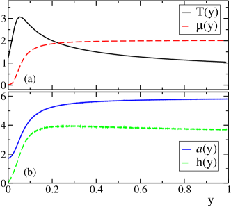
Figure 5: (Color online) (a) Temperature and chemical potential profiles as a function of $y=i/N$ for a chain of $N=3200$ sites and $T_{L}=T_{R}=1$, $\mu_{L}=0$, $\mu_{R}=2$. Each point is an average of the appropriate microcanonical expression derived from Eq. (5) over a subchain of about 10 sites around $i$. (b) Norm and energy densities corresponding to the profiles in (a).

In order to understand the onset of such anomalous shape, it is convenient to rewrite Eq. (9) by referring to $T$ and $\mu$. By introducing vector notations, we can write,

$${\bf J}={\bf A}(\mu,T)\frac{d{\bf v}}{dy}$$ (12)

where ${\bf J}=(j_{a},j_{h})$, ${\bf v}=(\mu,T)$, while the matrix ${\bf A}$ (which is no longer symmetric) can be expressed in terms of the Onsager matrix and of the fields $T$ and $\mu$ (for instance, $A_{11}=-L_{aa}/T$). By now inverting the above equation one obtains

$$\frac{d{\bf v}}{dy}={\bf A}^{-1}(\mu,T){\bf J}$$ (13)

where ${\bf A}^{-1}$ denotes the inverse of $\bf A$. This system describes a set of two linear differential equations which are non-autonomous (since the matrix coefficients in general vary with $\mu$ and $T$).

If one assumes to know the “material” properties (i.e. the matrix ${\bf A}^{-1}$) and wishes to determine fluxes and profiles, can proceed by integrating the differential equations, starting from the initial condition $T(0)=T_{L}$, $\mu(0)=\mu_{L}$. The, a priori unknown, parameters $j_{a}$ and $j_{h}$ can be determined by imposing that the final condition is $T(1)=T_{R}$ and $\mu(1)=\mu_{R}$. Alternatively, if the fluxes are known, one can integrate the equations up to any point $y_{0}$, and thereby generate the profiles that would be obtained by attaching the right end of the chain to thermal baths with temperature $T_{R}=T(y_{0})$ and chemical potential $\mu_{R}=\mu(y_{0})$.

In order to check the validity of the method, we have also adopted an alternative point of view, by combining the knowledge of the fluxes with simulations of short chains and small gradients to determine the elements of the matrix $A$ in suitably selected points in the $(T,\mu)$ plane. In order to estimate the four entries of $A$, it is necessary to perform two independent simulations for,

$$\left\{\begin{array}[]{ccc}T_{L,R}&=&T\pm\Delta T\\ \mu_{L,R}&=&\mu\end{array}\right.\ \ \ \left\{\begin{array}[]{ccc}T_{L,R}&=&T\\ \mu_{L,R}&=&\mu\pm\Delta\mu\end{array}\right.$$

With such information, we have been able to estimate $dv_{i}/dy$ along the chain (from Eq. (13)) and to compare the results with the direct simulations. The results plotted in Fig. 6 demostrate that the two approaches are in excellent agreement.

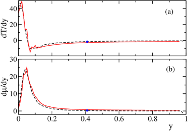
Figure 6: (Color online) Spatial derivatives of $T$ and $\mu$ (panels (a) and (b), respectively) computed from the profiles of Fig. 5 (black dashed lines) and their reconstruction (red solid lines) by Eq. (13) using the linear response coefficients (matrix $A$). The latter have been calculated on a chain of $N=250$. The quality of the recostruction improves by increasing the lattice size has shown by tha blue filled dot which is obtained for $N=1000$.

V Zero flux curves

A compact pictorial representation of transport properties is obtained by drawing the lines corresponding to vanishing fluxes $j_{a}$ and $j_{h}$. They can be directly determined by means of the conservative thermostats presented in Sec. II. Some lines are plotted in Fig. 7 both in the plane $(a,h)$ and $(T,\mu)$. It is worth recall that in the absence of a mutual coupling between the two transport processes (zero off-diagonal elements of the Onsager matrix) such curves would be vertical and horizontal lines in the latter representation. It is instead remarkable to notice that the solid lines, which correspond to $j_{h}=0$ are almost veritical for large $\mu$: this means that in spite of a large temperature difference, the energy flux is very small. This is an indirect but strong evidence that the nondiagonal terms are far from negligible.

The condition of a vanishing particle flux $j_{a}=0$ defines the Seebeck coefficient which is $S=-d\mu/dT$. Accordingly, the points where the dashed curves are vertical in Fig. 7b identify the locus where $S$ changes sign. The $j_{h}=0$ curves have no direct interpretation in terms of standard transport coefficients. Finally, if one connects a DNLS chain with any two points in the $(\mu,T)$ plane, its profile would correspond to the only path that is characterized by a constant ratio of $j_{a}/j_{h}$.

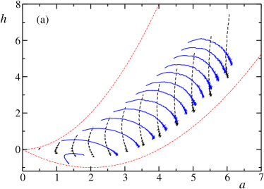
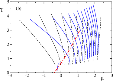
Figure 7: (Color online) Zero-flux curves in the $(a,h)$ and $(\mu,T)$ planes (panels (a) and (b), respectively). Black dashed and blue solid lines correspond to $j_{a}=0$ and $j_{h}=0$ respectively. Simulation are for a chain of length $N=500$. The thin dashed lines in the upper panel are the $T=0$ and $T=\infty$ isothermals. The thick dot-dashed line identify the locus where $S$ changes sign (see text).

It is instructive to compare these results with the scenario expected in the “harmonic” limit, where the nonlinear terms in the DNLS are negligible. Here, the dynamics is characterized by an ensemble of freely propagating waves and transport is thus ballistic. A direct reconstruction of the zero-flux lines by direct simulations is not very useful, as, in analogy with the known behaviour for the harmonic chain Rieder et al. (1967), the profiles of $T$ and $\mu$ are flat (except for a few sites close to the boundaries). Thus, the curves degenerate to single points and no comparison is possible. We thus resort to a different method of computing transport coefficients for ballistic systems, which is completely analogous to the well-know Landauer theory of electronic transport Sheng (2006). Consider an $N$-site chain in between two leads at different temperatures and chemical potentials $(T_{L},\mu_{L})$, $(T_{R},\mu_{R})$. Since transport is ballistic, energy and norm are carried by $N$ independent phonon modes, whose dispersion law is $\omega(q)=2\cos q$, $q$ being the wavenumber ($|q|\leq\pi$). Accordingly, the fluxes are $N$-independent and the ensuing transport coefficients are proportional to $N$. In this context, the norm and energy fluxes are given (up to some numerical constant) by the formulae

$$J_{a} = \int_{-2}^{+2}\,d\omega\,t(\omega)[f_{L}(\omega)-f_{R}(\omega)]$$

$$J_{h} = \int_{-2}^{+2}\,d\omega\,\omega\,t(\omega)\,[f_{L}(\omega)-f_{R}(\omega)]\,,$$

where $t(\omega)$ denotes the transmission coefficient, while $f_{L,R}$ are the equilibrium distribution functions of the reservoirs. If we assume that they are composed of two infinite linear chains (both with the same dispersion), the equipartition principle implies that the distributions are of the Rayleigh-Jeans form Rumpf (2004), $f_{L,R}(\omega)=f(T_{L,R},\mu_{L,R},\omega)$ where

$$f(T,\mu,\omega)=\frac{T}{\omega-2\mu}\quad,$$

(the factor 2 stems from the definition of $z_{n}$ and Eq. (3)) The physical meaning of the formulae is pretty intuitive: they can be derived from suitable generalized Langevin equations Iubini et al. following similar steps as for coupled oscillators, see e.g. Ref. Dhar and Roy (2006). The relevant information is contained in the transmission coefficient, that depends on how the chain is coupled to the external leads. For the Monte-Carlo bath we have used throughout this paper, the precise form of $t$ is not known. We thus postulate the simplest possible form, namely that, for large $N$, $t(\omega)=t$ for $|\omega|<2$ and zero otherwise. For our purposes, we set $t=1$ in the following, otherwise all the coefficients must be multiplied by $t$. If we introduce the function

$$\Phi(T,\mu)\equiv\int_{-2}^{+2}\,d\omega\,f(T,\mu,\omega)=T\ln\left(\frac{\mu-1}{\mu+1}\right)$$

which for $\mu<-1$ and $T>0$ is always positive, we can write,

$$J_{a} = \Phi(T_{L},\mu_{L})-\Phi(T_{R},\mu_{R})$$

$$J_{h} = 4(T_{L}-T_{R})+2\mu_{L}\Phi(T_{L},\mu_{L})-2\mu_{R}\Phi(T_{R},\mu_{R})\,.$$

By expanding to first order in $\Delta T=(T_{L}-T_{R})$ and $\Delta\mu=(\mu_{L}-\mu_{R})$

$$J_{a} = M_{00}\Delta T+M_{01}\Delta\mu$$

$$J_{h} = M_{10}\Delta T+M_{11}\Delta\mu\,$$ (14)

where

$$M=\left(\begin{array}[]{cc}\Phi(T,\mu)&\frac{2T}{\mu^{2}-1}\\ 4+2\mu\Phi(T,\mu)&\frac{4T\mu}{\mu^{2}-1}+2T\Phi(T,\mu)\end{array}\right).$$

With the help of the explicit formulae (14) we can reconstruct the zero-flux curves as follows. Starting from an initial point $(T_{in},\mu_{in})$ we compute $\Delta T$ and $\Delta\mu$ inverting Eqs. (14) setting $J_{a}=0,J_{h}=1$ and $J_{a}=1,J_{h}=0$, respectively (the value 1 is arbitrary). We then let $(T_{in},\mu_{in})\to(T_{in}+\Delta T,\mu_{in}+\Delta\mu)$ and iterate the procedure until the whole lines are reconstructed.

The results are depicted in Fig. 8. The curves for the linear case are defined only in the region $\mu<-1$. The results of the simulations of the DNLS (solid lines) nicely approach the curves of the linear case (dashed lines) upon decreasing $\mu$. The agreement is satisfactory, expecially in view of the many ad hoc assumptions made in deriving Eqs. (14).

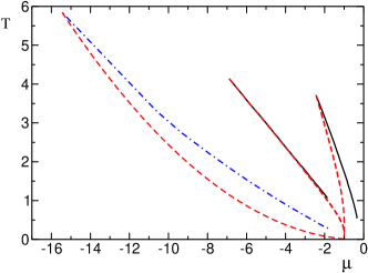
Figure 8: (Color online) Comparison of the zero-flux lines obtained from simulation of the DNLS equations (black solid and blue dot-dashed lines correspond to $j_{a}=0$ and $j_{h}=0$ respectively). The dashed (red) lines are the zero-flux lines computed by the Landauer formulae as described in the text.

VI Conclusions

We have presented the first study of stationary transport properties of the DNLS equation. Due to the nonstandard form of its Hamiltonian, several new issues have been brought to the fore that had not been addressed before in the literature dealing with energy transport in oscillator chains. In particular, we have extended the microscopic definition of the temperature to the chemical potential and defined suitable Monte Carlo thermostating schemes to characterize the nonequilibrium steady states of the DNLS in various regimes. The simulations confirm the expectations that transport is normal (i.e. the Onsager coefficients are finite in the thermodynamic limit), although some almost ballistic transport is found at very low temperature, where the DNLS approaches an almost integrable limit.

Due to the very existence of two naturally coupled transport processes, the nonequilibrium steady state can display nonmonotonous energy and density profiles. To our knowledge, this unusual feature has not been observed so far in any other oscillator or particle model. As seen from Eq. (13), it is clear that the temperature profile cannot in general be linear in $y$, since the elements of ${\bf A}^{-1}$ depend on $\mu$ and $T$. In principle, the profiles may have have nontrivial shapes depending on the qualitative behaviour of the solutions of Eq. (13). In the DNLS, the phenomenon is particularly pronounced (the temperature inside the chain reaches values that are almost three times larger than those imposed by the thermal baths) because of the strong variability of the Onsager coefficients. It would be interesting to find the physical motivation for this effect to predict and possibly control the conditions for its appearance.

Another novel feature is the fact that the Seebeck coefficient changes sign upon changing the state parameters e.g. by increasing the interaction strength. The observable consequence of this is that the temperature and chemical potential gradients change their relative signs. As the particle density $a$ increases with $\mu$ this also implies that $a$ may be larger in the colder regions.

Furthermore, a remakable feature of the DNLS thermodynamics is the possibility of negative temperatures states in suitable parameter regions Rasmussen et al. (2000a). These regions, that are characterized by the presence of long-lived localized excitations (discrete breathers), have not be considered in the present paper, but are definitely worth being explored. It may be indeed speculated that they would lead to genuine nonlinear transport features and even to the birth of new dynamical regimes possibly displaying transitions between conducting and insulating states.

Besides its intrinsic theoretical interest as a testbed for the characterization of coupled irreversible processes, the DNLS equation opens the way also to experimental investigations. In fact, despite its mathematical simplicity, the DNLS model can be of guidance in the design and interpretation of experiments on coupled-transport in cold atomic gases in deep optical lattices as well as in optical multilayered and nonlinear structures.