Coexistence and competition of nematic and gapped states in bilayer graphene

Abstract

In bilayer graphene, the phase diagram in the plane of a strain-induced bare nematic term, ${\cal N}_{0}$, and a top-bottom gates voltage imbalance, $U_{0}$, is obtained by solving the gap equation in the random-phase approximation. At nonzero ${\cal N}_{0}$ and $U_{0}$, the phase diagram consists of two hybrid spin-valley symmetry-broken phases with both nontrivial nematic and mass-type order parameters. The corresponding phases are separated by a critical line of first- and second-order phase transitions at small and large values of ${\cal N}_{0}$, respectively. The existence of a critical end point, where the line of first-order phase transitions terminates, is predicted. For ${\cal N}_{0}=0$, a pure gapped state with a broken spin-valley symmetry is the ground state of the system. As ${\cal N}_{0}$ increases, the nematic order parameter increases, and the gap weakens in the hybrid state. For $U_{0}=0$, a quantum second-order phase transition from the hybrid state into a pure gapless nematic state occurs when the strain reaches a critical value. A nonzero $U_{0}$ suppresses the critical value of the strain. The relevance of these results to recent experiments is briefly discussed.

I Introduction

At present, a significant amount of attention is being paid to the ground state of bilayer graphene at the neutrality point. Various gapped states with broken spin-valley symmetry, such as quantum anomalous Hall (QAH),QAH quantum spin Hall (QSH),QSH quantum valley Hall (QVH),QVH layer antiferromagnet (LAF),Zhang as well as a gapless nematic state,Vafek ; Lemonik were suggested as candidates for the ground state. ExperimentsWeitz ; Freitag ; Velasco1 ; Velasco2 showed that bilayer graphene at the neutrality point is gapped in the absence of external fields. However, the experiment performed by the Manchester groupMayorov found a gapless state, and there were strong indications that it was a nematic state.

A variety of suggested ground states is related to the way in which the approximate $SU(4)$ spin-valley symmetry of the low energy effective model of bilayer graphene is broken in its ground state. The application of external electric and magnetic fields adds more complexity to the problem of the ground state of bilayer graphene. However, it opens the possibility to use them as useful probes of the ground state of the system. Theoretical papersGGM ; Levit ; Toke predicted and experimentsWeitz ; Kim ; Velasco1 ; Velasco2 showed the presence of a phase transition between the QSH and the QVH states as an electric field increases. Since the QVH (layer polarized) state is the ground state of the system for a sufficiently large electric field, this rules out the QVH state as a candidate for the ground state in the absence of external fields.

Simple continuity arguments suggest that the LAF and QSH states are the most likely candidates for the gapped ground state of bilayer graphene at the neutrality point in the absence of external fields. Indeed, for a sufficiently large magnetic field, the QSH (spin polarized) state is the ground state of bilayer graphene. On the other hand, the experimentsFreitag ; Velasco1 ; Velasco2 do not show any phase transitions in bilayer graphene at the neutrality point as a magnetic field is switched off. This excludes the QAH state because it cannot be smoothly connected to the spin polarized state at large magnetic fields. The LAF state, on the other hand, can adiabatically evolve into the QSH oneKharitonov and, therefore, cannot be excluded.

In Refs. QVH, and MacD, , it was shown that, unlike single-layer graphene with its linear dispersion relation, the quadratic dispersion relation in bilayer graphene leads to an instability of its normal phase for arbitrary weak Coulomb or short-range repulsive interactions. Renormalization group studies in the normal phase of bilayer graphene in Refs. Vafek, and Lemonik, revealed a variety of instabilities in this phase, which can potentially lead to different (competing) ground states with condensates. It was also found that the instability with respect to the generation of a nematic order parameter is strongest, which seems to suggest that the nematic state is the ground state of bilayer graphene. However, since the condensates essentially modify the gap equations, in order to determine the phase diagram of the system, it is necessary to analyze the gap equations for states with different condensates and then to compare their energy densities. This is the main goal of the present paper.

Solving the gap equation in the random-phase approximation, we find the phase diagram in the plane of a strain-induced bare nematic term ${\cal N}_{0}$ and a top-bottom gates voltage imbalance $U_{0}$. We show that the ground state of the system at ${\cal N}_{0}\neq 0$ and $U_{0}\neq 0$ is a hybrid state with nonzero nematic and mass-type order parameters. The critical line separates the phase with one of the hybrid QAH, QSH, or LAF states (which are degenerate in energy in the model at hand) from the hybrid QVH state. The phase transition along a large part of this critical line is of second-order except for the region of small ${\cal N}_{0}$ where a sufficiently large value of $U_{0}$ drives the first-order phase transition between the two different states with broken spin-valley symmetry. The predicted existence of a critical end point in the phase diagram may be relevant to current experiments in bilayer graphene.

The paper is organized as follows. The analysis is performed in the framework of the two-band model of bilayer graphene with the Coulomb interaction between quasiparticles described in Sec. II. In Sec. III we derive the gap equations in the random-phase approximation for the gapped and nematic order parameters. The main results of the paper, including the numerical solutions to the gap equations, are presented in Sec. IV. Sec. V contains a brief summary of the results, as well as our discussions and conclusions. In the Appendix the derivation of the expression for the energy density is given.

II Model

The free part of the effective low-energy Hamiltonian of bilayer graphene is as follows:McC

$$H_{0}=-\frac{1}{2m}\sum_{\xi,s}\int d^{2}x\,\Psi_{\xi s}^{+}(x)\left(\begin{array}[]{cc}0&(\pi^{\dagger})^{2}\\ \pi^{2}&0\end{array}\right)\Psi_{\xi s}(x),$$ (1)

where $\pi=\hat{k}_{1}+i\hat{k}_{2}$ is the canonical momentum operator, $m=\gamma_{1}/2v_{F}^{2}$, where the Fermi velocity is $v_{F}\simeq c/300$, and $\gamma_{1}\approx 0.4~{}\mbox{eV}$. The two-component spinor field $\Psi_{\xi s}$ carries the valley $(\xi=\pm$ for $K$ and $K^{\prime}$ valleys, respectively) and spin ($s=\pm$) indices. We will use the standard convention:McC $\Psi_{+s}^{T}=(\psi_{+A{{}_{1}}},\psi_{+B{{}_{2}}})_{s}$, whereas, $\Psi_{-s}^{T}=(\psi_{-B{{}_{2}}},\psi_{-A{{}_{1}}})_{s}$. Here, $A_{1}$ and $B_{2}$ correspond to those sublattices in layers 1 and 2, respectively, which, according to Bernal $(A_{2}-B_{1})$ stacking, are relevant for the low energy dynamics. Let us emphasize that the sublattice and layer degrees of freedom are not independent in this low-energy model: The sublattices $A_{1}$ and $B_{2}$ correspond to layers $1$ and $2$, respectively. The effective Hamiltonian (1) is valid up to energies $\Lambda=\gamma_{1}/4\approx 0.1~{}\mbox{eV}$ and we ignore small trigonal warping effects.McC

The Coulomb interactions in bilayer graphene are given byQVH ; GGM

$$H_{C}=\frac{1}{2}\int d^{2}xd^{2}x^{\prime}\Big{\{}V(x-x^{\prime})\left[\rho_{1}(x)\rho_{1}(x^{\prime})+\rho_{2}(x)\rho_{2}(x^{\prime})\right]$$

$$\hskip 71.13188pt+2V_{12}(x-x^{\prime})\rho_{1}(x)\rho_{2}(x^{\prime})\Big{\}},$$ (2)

where the interaction potentials $V(x)$ and $V_{12}(x)$ describe the intralayer and interlayer interactions, respectively. Their Fourier transforms are ${V}(k)=2\pi e^{2}/\kappa k$ and ${V}_{12}(k)=2\pi e^{2}e^{-kd}/\kappa k$, where $d\approx 0.35~{}\mbox{nm}$ is the distance between the layers, and $\kappa$ is a dielectric constant (in the numerical analysis below, we set $\kappa=4$). The two-dimensional charge-density operators $\rho_{1}(x)$ and $\rho_{2}(x)$ are

$$\rho_{l}(x)=\sum_{\xi,s=\pm}\Psi^{+}_{\xi s}(x)P_{l}(\hat{\xi})\Psi_{\xi s}(x),\quad(l=1,2),$$ (3)

where $P_{1}(\hat{\xi})=(1+\hat{\xi}\tau^{3})/2$ and $P_{2}(\hat{\xi})=(1-\hat{\xi}\tau^{3})/2$ are projectors on states in the layers 1 and 2, respectively. Here the matrix $\hat{\xi}$ acts as $\hat{\xi}\Psi_{\xi s}=\xi\Psi_{\xi s}$, and $\tau^{3}$ is the diagonal Pauli matrix acting on the two components of the fields $\Psi_{+s}$ and $\Psi_{-s}$. Note that the presence of $\hat{\xi}$ in $P_{1}(\hat{\xi})$ and $P_{2}(\hat{\xi})$ is related to the opposite order of the $A_{1}$ and $B_{2}$ components in $\Psi_{+s}$ and $\Psi_{-s}$.

Whereas, the gaps in the QAH and QSH states in bilayer graphene are analogous to a Haldane mass,QAH ; QSH the gaps in the QVH and LAF states are analogous to a Dirac mass.Zhang ; GGM In bilayer graphene, the latter is realized as a voltage imbalance between the layers.GGM ; McC The corresponding order parameters (condensates) are as followsZhang ; GGM : spin singlets $\langle\Psi^{\dagger}\tau^{3}\Psi\rangle$ (QAH) and $\langle\Psi^{\dagger}\hat{\xi}\tau^{3}\Psi\rangle$ (QVH), and spin triplets $\langle\Psi^{\dagger}\tau^{3}\sigma^{3}\Psi\rangle$ (QSH) and $\langle\Psi^{\dagger}\hat{\xi}\tau^{3}\sigma^{3}\Psi\rangle$ (LAF), where $\sigma_{3}$ is a spin Pauli matrix (the indices $\xi$ and $s$ in the field $\Psi_{\xi s}$ are omitted here).

Without a magnetic field, the QSH and QVH states are invariant under time reversal,QSH ; QVH whereas, the QAH and LAF states break this symmetryQAH ; Zhang (the QAH state is associated with the Chern number QAH and the QSH state is a two-dimensional topological insulator associated with the $Z_{2}$ topological invariant QSH ). On the other hand, although the QAH state is invariant under the $SU(4)$, the QSH one breaks the spin $SU(2)$ subgroup of $SU(4)$ down to $U(1)$.QSH ; GGM Both the QVH and the LAF states break a $Z_{2}$ subgroup of the spin-valley $SU(4)$ describing the valley transformation $\xi\to-\xi$ ($\Psi_{+s}\to\Psi_{-s}$),GGM in addition to that, the LAF state breaks the spin $SU(2)$ down to $U(1)$.

A usual nematic order parameter breaks the $SO(2)$ rotational group down to a discrete $Z_{2}$ subgroup. As we discuss below, however, nematic ordering in bilayer graphene may become hybridized with the ordering of spin-valley symmetry-broken states. As a result, there can exist four different types of nematic ordering. The corresponding expressions for the nematic order parameters (condensates) can be formally obtained from those in the spin-valley symmetry-broken gapped phases by replacing the matrix $\tau^{3}$ with $\tau^{1}$, i.e., they are given by the following anisotropic order parameters: $\langle\Psi^{\dagger}\tau^{1}\Psi\rangle$, $\langle\Psi^{\dagger}\tau^{1}\sigma^{3}\Psi\rangle$, $\langle\Psi^{\dagger}\hat{\xi}\tau^{1}\Psi\rangle$, and $\langle\Psi^{\dagger}\hat{\xi}\tau^{1}\sigma^{3}\Psi\rangle$. These generalized nematic order parameters break the continuous spin-valley symmetry in the same fashion as the corresponding order parameters in the QAH, QSH, QVH and LAF phases, respectively. Also, although two of them, $\langle\Psi^{\dagger}\tau^{1}\sigma^{3}\Psi\rangle$ and $\langle\Psi^{\dagger}\hat{\xi}\tau^{1}\Psi\rangle$, are invariant under time reversal, the other two, $\langle\Psi^{\dagger}\tau^{1}\Psi\rangle$ and $\langle\Psi^{\dagger}\hat{\xi}\tau^{1}\sigma^{3}\Psi\rangle$ break this symmetry. From a physics viewpoint, different types of nematic ordering are possible when quasiparticles with different spins and valleys contribute unequally to the nematic condensates. In states with broken spin-valley symmetries, this should be, of course, generally expected.

III Quasiparticle propagator and gap equation

Our goal is to solve the Schwinger–Dyson (gap) equation for the quasiparticle propagator in the spin-valley symmetry-broken gapped states as well as gapless nematic states using a unified framework. In general, the full quasiparticle propagator in the coordinate space at fixed valley and spin is defined by

$$G_{\xi s}(x-x^{\prime})=-i\langle 0|T\Psi_{\xi s}(x)\Psi^{\dagger}_{\xi s}(x^{\prime})|0\rangle.$$ (4)

In the random-phase approximation, the corresponding gap equation is readily obtained from the Baym-Kadanoff functional in the two-loop approximation, see Eq. (9) in the second paper in Ref. GGM, ,

$$G^{-1}_{\xi s}(x-x^{\prime}) = S^{-1}_{\xi s}(x-x^{\prime})-iG_{\xi s}(x-x^{\prime})V_{\rm eff}(x-x^{\prime})$$ (5)

$$- i\left[P_{1}(\xi)G_{\xi s}(x-x^{\prime})P_{2}(\xi)+P_{2}(\xi)G_{\xi s}(x-x^{\prime})P_{1}(\xi)\right]V_{\rm IL}(x-x^{\prime})$$

$$- \frac{i}{2}\delta^{3}(x-x^{\prime})\left[P_{1}(\xi)-P_{2}(\xi)\right]\sum_{\xi^{\prime},s^{\prime}=\pm}\mbox{tr}\left\{\left[P_{1}(\xi^{\prime})-P_{2}(\xi^{\prime})\right]G_{\xi^{\prime}s^{\prime}}(x-x^{\prime})\right\}\tilde{V}_{\rm IL}(0),$$

where $x=(t,\mathbf{x})$ and the trace is taken over the spinor components of the quasiparticle propagator. The dynamically screened interactions $V_{\rm eff}$ and $V_{\rm IL}$ are defined by Eqs. (A5) and (A6) in the second paper of Ref. GGM, , $\tilde{V}_{\rm IL}(0)=-2\pi e^{2}d/\kappa$ is the Fourier transform of the bare interaction $V^{\rm bare}_{\rm IL}(x)$ taken at $\omega=\mathbf{k}=0$. The explicit form of the inverse free propagator in momentum space reads

$$S^{-1}_{\xi s}(\omega,\mathbf{k})=\left(\begin{array}[]{cc}\omega-\xi U_{0}&\frac{k^{2}}{2m}e^{-2i\varphi_{k}}+{\cal N}_{0}\\ \frac{k^{2}}{2m}e^{2i\varphi_{k}}+{\cal N}_{0}&\omega+\xi U_{0}\end{array}\right),$$ (6)

where $\varphi_{k}$ is a polar angle of the quasiparticle momentum with respect to the orientation of the nematic order, $U_{0}=eE_{\perp}d/2$ is the top-bottom gates voltage imbalance, $E_{\perp}$ is the electric field perpendicular to the layers, and ${\cal N}_{0}$ is the bare nematic order parameter due to strainref1 and rotational mismatchref2 between the layers of bilayer graphene. Its value is related, for example, to the angle of rotational mismatch $\theta$ as follows:ref2

$${\cal N}_{0}=\left(\frac{\hbar v_{F}}{2a}\right)^{2}\frac{\theta^{2}}{\gamma_{1}},$$ (7)

where $a=0.142$ nm is the intralayer distance between neighboring carbon atoms.

The Fock contribution is given by the second and third terms on the right-hand side of Eq. (5), whereas, the fourth term describes the Hartree contribution. [Note that, in accordance with Gauss’s law, we omitted the Hartree contribution connected with the total electron charge of the system proportional to $\sum_{\xi,s}\mbox{tr}[G_{\xi s}(0)]$, which is neutralized by the positive charges of ions in the system.] Taking into account that $\langle\rho_{l}\rangle=-i\,\sum_{\xi,s}\mbox{tr}[P_{l}(\xi)\,G_{\xi s}(0)]$ defines the electron charge density in the $l$th layer, we see that the Hartree term proportional to the $\tilde{V}_{\rm IL}(0)$ interaction describes the layer charge-density imbalance. One of the Fock terms in Eq. (5) is proportional to $V_{\rm IL}$. Since $V_{\rm IL}\sim d$, it is suppressed compared to the one with $V_{\rm eff}$. Because of the polarization effects, $V_{\rm IL}$ is also suppressed compared to $V^{\rm bare}_{\rm IL}$.QVH Therefore, it is justifiable to neglect the Fock term with the $V_{\rm IL}$ interaction in the analysis that follows.

Taking into account the gapped and nematic order parameters in the inverse quasiparticle propagator at fixed valley and spin, we use the following ansatz:

$$G^{-1}_{\xi s}(\omega,\mathbf{k})=\left(\begin{array}[]{cc}Z^{-1}(\omega,\mathbf{k})\omega-\xi\Delta_{\xi s}(\omega,\mathbf{k})&\frac{k^{2}}{2m}A(\omega,\mathbf{k})e^{-2i\varphi_{k}}+w_{\xi s}(\omega,\mathbf{k})\\ \frac{k^{2}}{2m}A(\omega,\mathbf{k})e^{2i\varphi_{k}}+w_{\xi s}(\omega,\mathbf{k})&Z^{-1}(\omega,\mathbf{k})\omega+\xi\Delta_{\xi s}(\omega,\mathbf{k})\end{array}\right)\,,$$ (8)

where $k$ and $\varphi_{k}$ are polar coordinates in the $(k_{1},k_{2})$ plane. Note that although, in general, $w_{\xi s}$ is a complex function, one can show that, without the loss of generality, its phase can be set to zero. The functions $Z(\omega,\mathbf{k})$ and $A(\omega,\mathbf{k})$ define quasiparticle residue at the pole and renormalization of the kinetic term, respectively.

In Eq. (8), $\Delta_{\xi s}=U_{s}+\xi\Delta_{s}$ and $w_{\xi s}={\cal N}_{s}+\xi{\cal M}_{s}$ are the spin-valley symmetry-breaking and nematic parameters, which are connected to the order parameters discussed above through the following relationship:

$$\langle\Psi^{\dagger}{\cal O}\Psi\rangle=-i\sum_{\xi,s}\int\frac{d\omega d^{2}k}{(2\pi)^{3}}{\rm tr}[{\cal O}G_{\xi,s}(\omega,\mathbf{k})].$$ (9)

Here the matrix ${\cal O}$ is $\tau^{3}$, $\tau^{3}\sigma^{3}$, $\hat{\xi}\tau^{3}$, and $\hat{\xi}\tau^{3}\sigma^{3}$ for the QAH, QSH, QVH, and LAF order parameters, respectively, and ${\cal O}=\tau^{1}$, $\tau^{1}\sigma^{3}$, $\hat{\xi}\tau^{1}$, and $\hat{\xi}\tau^{1}\sigma^{3}$ for nematic order parameters. [In Eq. (9), the trace runs over the valley degree of freedom.] For the QSH state at $U_{0}=0$ and ${\cal N}_{0}=0$, only the spin-triplet Haldane mass ($\Delta_{+}=-\Delta_{-}$) is nonzero in $\Delta_{\xi s}$. On the other hand, for the QAH state, only the spin-singlet Haldane mass ($\Delta_{+}=\Delta_{-}$) is nonzero. Similarly, only the spin-antisymmetric part of $U_{s}$, $U_{+}=-U_{-}$, describes the LAF state, and the symmetric in spin voltage $U_{+}=U_{-}$ occurs in the QVH state. In fact, at $U_{0}=0$ these definitions remain unchanged even in the corresponding hybrid states, in which an additional spin-singlet nematic parameter ${\cal N}_{+}={\cal N}_{-}$ is induced by the bare nematic term ${\cal N}_{0}$.

When $U_{0}\neq 0$, however, the most general hybrid QSH, QAH and LAF phases get further modified. In the hybrid QSH state, for example, there will appear a nonzero contribution of a spin-symmetric parameter $U_{+}=U_{-}$ and a spin-antisymmetric parameter ${\cal M}_{+}=-{\cal M}_{-}$. In the hybrid QAH state, the admixture of two spin-singlet parameters $U_{+}=U_{-}$ and ${\cal M}_{+}={\cal M}_{-}$ will appear. Finally, in the hybrid LAF state, the new nonzero contributions will be a spin-symmetric parameter $U_{+}=U_{-}$ and a spin-antisymmetric parameter ${\cal N}_{+}=-{\cal N}_{-}$.

Although $\Delta_{\xi s}$ and $w_{\xi s}$ can, in general, be energy and momentum dependent, in our analysis, we use the constant approximation for them. Also, we set $Z(\omega,\mathbf{k})=A(\omega,\mathbf{k})=1$ in $G^{-1}_{\xi s}(\omega,\mathbf{k})$ in Eq.(8). Then, the propagator reads

$$G_{\xi s}(\omega,\mathbf{k})=\frac{1}{\omega^{2}-\frac{k^{4}}{4m^{2}}-\Delta^{2}_{\xi s}-w^{2}_{\xi s}-\frac{k^{2}w_{\xi s}\cos 2\varphi_{k}}{m}+i0}\,\left(\begin{array}[]{cc}\omega+\xi\Delta_{\xi s}&-\frac{k^{2}}{2m}e^{-2i\varphi_{k}}-w_{\xi s}\\ -\frac{k^{2}}{2m}e^{2i\varphi_{k}}-w_{\xi s}&\omega-\xi\Delta_{\xi s}\end{array}\right)\,.$$ (10)

The poles of this propagator determine the dispersion relations of quasiparticles,

$$\omega_{\xi,s,\pm}=\pm\sqrt{\left(\frac{k^{2}}{2m}-w_{\xi s}\right)^{2}+\frac{k^{2}}{m}w_{\xi s}\left(1+\cos 2\varphi_{k}\right)+\Delta^{2}_{\xi s}}.$$ (11)

As we see, a nonzero dynamical parameter $\Delta_{\xi s}$ results in a fully gapped dispersion relation for the quasiparticles with fixed $\xi$ and $s$. When $\Delta_{\xi s}=0$, in contrast, the quasiparticles with $k=\sqrt{2m|w_{\xi s}|}$ have a vanishing gap for $\varphi_{k}=\pm\pi/2$ and $w_{\xi s}>0$, and for $\varphi_{k}=0,\pi$ when $w_{\xi s}<0$.

Multiplying the Schwinger–Dyson equation (5) by $\tau_{3}$ and $\tau_{1}$ Pauli matrices, respectively, taking the trace over the spinor components, and making the Wick rotation, we obtain the following set of gap equations for $\Delta_{\xi s}$ and $w_{\xi s}$:

$$\Delta_{\xi s}=U_{0}+\int\frac{d\omega d^{2}k}{(2\pi)^{3}}\frac{\Delta_{\xi s}}{D_{\xi s}(\omega,k)}V_{\rm eff}(\omega,k)+\frac{1}{2}\delta\rho\tilde{V}_{\rm IL}(0)\,,$$ (12)

$$w_{\xi s}={\cal N}_{0}+\int\frac{d\omega d^{2}k}{(2\pi)^{3}}\frac{w_{\xi s}+\frac{k^{2}}{2m}\cos 2\varphi_{k}}{D_{\xi s}(\omega,k)}V_{\rm eff}(\omega,k),$$ (13)

where

$$\delta\rho\equiv\langle\rho_{2}-\rho_{1}\rangle=\sum_{\xi,s=\pm}\int\frac{d\omega d^{2}k}{(2\pi)^{3}}\frac{2\Delta_{\xi s}}{D_{\xi s}(\omega,k)}$$ (14)

is the charge density imbalance between the layers and

$$D_{\xi s}(\omega,k)=\omega^{2}+\Delta^{2}_{\xi s}+w^{2}_{\xi s}+\frac{k^{4}}{4m^{2}}+\frac{k^{2}w_{\xi s}\cos 2\varphi_{k}}{m}\,.$$ (15)

In the effective potential $V_{\rm eff}(\omega,k)$ in Eqs. (12) and (13), we take into account the dynamical polarization of the Coulomb interaction,QVH

$$V_{\rm eff}(\omega,k)=\frac{2\pi e^{2}}{\kappa k+\frac{4e^{2}m\ln 4}{\sqrt{1+[{4m\omega\ln 4}/({\pi k^{2}})]^{2}}}}\,.$$ (16)

At fixed values of $U_{0}$ and ${\cal N}_{0}$, the gap equations (12) and (13) generally admit many solutions. In order to determine which of them corresponds to the ground state, we need to find the solution with the lowest energy density. The expression for the energy density is obtained in the Appendix.

It should be mentioned that, in the model at hand, which includes only the dominant Coulomb interaction and has no external magnetic field, the three types of solutions with spontaneous spin-valley symmetry breaking, QAH, LAF, and QSH, appear to be degenerate in energy. Moreover, the order parameters in these three phases are related by some transformations. This means, in particular, that having the explicit form for one of them allows for easily reconstructing the other two. For example, if the spin-singlet hybrid QAH solution is found to take the following form:

$$\Delta_{+}=\Delta_{-}=f_{1}(U_{0},{\cal N}_{0}),$$ (17)

$$U_{+}=U_{-}=f_{2}(U_{0},{\cal N}_{0}),$$ (18)

$${\cal N}_{+}={\cal N}_{-}=f_{3}(U_{0},{\cal N}_{0}),$$ (19)

$${\cal M}_{-}={\cal M}_{+}=f_{4}(U_{0},{\cal N}_{0}),$$ (20)

with the functions on the right-hand sides depending on $U_{0}$, ${\cal N}_{0}$ and other model parameters, the corresponding QSH and LAF solutions can be immediately determined as well. In particular, the QSH solution is given by

$$\Delta_{+}=-\Delta_{-}=f_{1}(U_{0},{\cal N}_{0}),$$ (21)

$$U_{+}=U_{-}=f_{2}(U_{0},{\cal N}_{0}),$$ (22)

$${\cal N}_{+}={\cal N}_{-}=f_{3}(U_{0},{\cal N}_{0}),$$ (23)

$${\cal M}_{+}=-{\cal M}_{-}=f_{4}(U_{0},{\cal N}_{0}),$$ (24)

whereas, the LAF solution is given by

$$\Delta_{+}=\Delta_{-}=0,$$ (25)

$$U_{\pm}=\frac{f_{2}(U_{0},{\cal N}_{0})\mp f_{1}(U_{0},{\cal N}_{0})}{2},$$ (26)

$${\cal N}_{\pm}=\frac{f_{3}(U_{0},{\cal N}_{0})\pm f_{4}(U_{0},{\cal N}_{0})}{2},$$ (27)

$${\cal M}_{-}={\cal M}_{+}=0\,.$$ (28)

IV Results

In this section, we present our main results. We start from the analysis of the gap equations in the case of vanishing top-bottom gates voltage imbalance, $U_{0}=0$. In particular, we reveal the emergence of the hybrid state at nonzero bare nematic parameter ${\cal N}_{0}$ and describe how it gradually turns into a pure nematic state with increasing ${\cal N}_{0}$. We then discuss the complete phase diagram in the $U_{0}$–${\cal N}_{0}$ plane.

IV.1 Nematic and spin-valley symmetry-broken states at $U_{0}=0$

In the hybrid QSH, QAH, and LAF states (with an addition of nematic ordering), we find that in general the nematic parameters depend on spin and/or valley indices, i.e., ${\cal N}_{+}\neq{\cal N}_{-}$ and ${\cal M}_{s}\neq 0$. However, in the case of the vanishing top-bottom gates voltage imbalance, $U_{0}=0$, the structure of $w_{\xi s}$ simplifies: ${\cal N}_{+}={\cal N}_{-}$ and ${\cal M}_{s}=0$. The latter follows from the structure of Eqs. (12), (13), and (15). In order to clarify the role of a bare nematic parameter ${\cal N}_{0}$ in competition between the nematic and the gapped states, we first study this case. Then, the numerical analysis of gap equations (12) and (13) shows that solutions of the two types are possible. One of them is the nematic solution with only $w_{\xi s}\neq 0$, and the other is a hybrid solution with both $\Delta_{\xi s}$ and $w_{\xi s}$ nonzero. Note that a gapped solution with only $\Delta_{\xi s}\neq 0$ is impossible when a nonzero bare nematic parameter ${\cal N}_{0}$ is present, therefore, gap and nematic parameters coexist in the hybrid solution.

At vanishing $U_{0}$ and ${\cal N}_{0}$, the QVH solution has a higher energy than the QAH, LAF, and QSH solutions. The additional energy cost is due to the Hartree term $\frac{1}{2}\delta\rho\tilde{V}_{\rm IL}$ in the gap equation (12). This term is negative because it reflects the energy price associated with the electric field between the layers of graphene in the QVH phase. Thus, there are two main solutions of the gap equations (12) and (13), the pure nematic and one of the hybrid solutions, QAH, LAF, or QSH. The latter are degenerate in energy. Instead of discussing all the degenerate solutions, in the rest of the paper, we will concentrate only on the hybrid QSH one.

In the pure nematic solution, the nematic order parameter ${\cal N}_{s}$ does not depend on the valley or the spin. Its dependence on the bare parameter ${\cal N}_{0}$ is shown in Fig. 1. At small ${\cal N}_{0}$, it can be approximated by a linear dependence ${\cal N}_{\pm}={\cal N}_{\rm off}+b{\cal N}_{0}$ with the offset ${\cal N}_{\rm off}=4.61\,\mbox{meV}$ and the slope $b=3.18$. For the hybrid QSH solution, the gaps $\Delta_{s}$ and ${\cal N}_{s}$ are also plotted in Fig. 1. We see that the bare nematic parameter inhibits the gap.

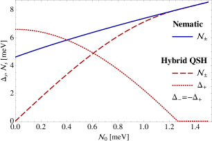
Figure 1: (Color online) The order parameters $\Delta_{s}$ and ${\cal N}_{s}$ as functions of the bare nematic term ${\cal N}_{0}$ for the nematic solution (solid line) and for the hybrid QSH solution (dashed and dotted lines) at $U_{0}=0$.

Comparing the energy densities of the nematic and hybrid QSH solutions, we find that the hybrid solution always has a lower free energy whenever it exists, see Fig. 2. From Fig. 1, we see that the dynamical nematic order parameter ${\cal N}_{s}$ for the hybrid QSH solution vanishes as ${\cal N}_{0}\to 0$. Therefore, the ground state of unbiased bilayer graphene at ${\cal N}_{0}=U_{0}=0$ is a spin-valley symmetry-broken gapped state. Whereas, the dynamical nematic order parameter ${\cal N}_{s}$ grows, the gap $\Delta_{s}$ gradually decreases with increasing the bare nematic parameter ${\cal N}_{0}$. Eventually, the hybrid QSH solution smoothly turns into the pure nematic solution at the critical point ${\cal N}^{\rm cr}_{0}\approx 1.26\,\mbox{meV}$ where the gap $\Delta_{s}$ turns to zero. Since the QSH state breaks the spin $SU(2)$ symmetry, whereas, the nematic state does not, we conclude that the corresponding transition is a second-order phase transition (and not a smooth crossover).

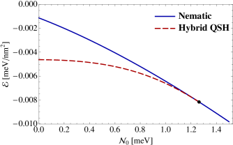
Figure 2: (Color online) The energy density as a function of the bare nematic term ${\cal N}_{0}$ for the nematic solution (solid line) and the hybrid QSH solution (dashed line) at $U_{0}=0$.

IV.2 Phase diagram

Using a coupled set of gap equations for the nematic and several types of spin-valley symmetry-breaking order parameters in bilayer graphene, we can now obtain a phase diagram in the plane of two parameters: a strain-induced bare nematic term ${\cal N}_{0}$ and a top-bottom gates voltage imbalance $U_{0}$. This is performed by sweeping through the corresponding two-dimensional space of the bare parameters, comparing the energies of all solutions, and determining the ground state at each point. The results are summarized in Fig. 3.

Figure 3: The phase diagram in the ${\cal N}_{0}$-$U_{0}$ plane.

To understand the overall topology of the phase diagram, it is useful to first look at the competition of the non-nematic phases at ${\cal N}_{0}=0$.GGM ; Levit ; Toke In this case, increasing the voltage imbalance $U_{0}$ has a tendency to suppress the QSH state gap $\Delta_{s}$ and to induce an increasing admixture of the $U_{s}$ gap in this state. At a sufficiently large $U_{0}$, a pure QVH state with a spin singlet $U_{s}$ gap takes over as the ground state.

In the subcritical region (i.e., at small values of ${\cal N}_{0}$ and $U_{0}$) of the phase diagram at a fixed $U_{0}\neq 0$, increasing the bare nematic term ${\cal N}_{0}$ induces a substantial dynamical nematic order parameter $w_{\xi s}$, see Fig. 4 for $U_{0}=0.4\,\mbox{meV}$. Consequently, in this case, the hybrid QSH state has spin-symmetric order parameters $U_{s}$ and ${\cal N}_{s}$, and spin asymmetric order parameters $\Delta_{s}$ and ${\cal M}_{s}$. In the supercritical region, the hybrid QVH state with spin singlet $U_{s}$ and ${\cal N}_{s}$ parameters (see Fig. 4) has the lowest energy. As expected, the hybrid QVH state becomes almost a pure nematic state at small $U_{0}$ and large ${\cal N}_{0}$ and almost a pure QVH state at large $U_{0}$ and small ${\cal N}_{0}$.

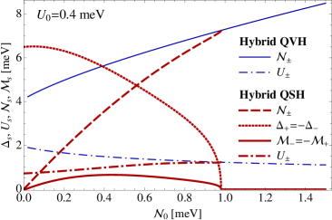
Figure 4: (Color online) The order parameters as functions of the bare nematic term ${\cal N}_{0}$ for the hybrid QSH solution (thick red lines) and hybrid QVH solution (thin blue lines) at $U_{0}=0.4\,\mbox{meV}$.

The critical line in Fig. 3 separates the hybrid QSH and QVH phases. Its top part corresponds to a first-order phase transition (the gaps of the hybrid QSH and QVH states are discontinuous across the critical line), which ends in a critical end point at ${\cal N}^{\star}_{0}\approx 0.36\,\mbox{meV}$ and $U^{\star}_{0}\approx 0.95\,\mbox{meV}$. The rest of the critical line corresponds to a second-order phase transition.

V Summary

The current paper shows that bilayer graphene has a rich phase diagram in the plane of the bare nematic term ${\cal N}_{0}$ and the voltage imbalance between the layers $U_{0}$.footnote2 It is argued that the ground state should be one of several hybrid states with spontaneous spin-valley symmetry breaking.

We find, in particular, that one of the hybrid states, QAH, LAF, or QSH state is the ground state in the subcritical region (i.e., small values of ${\cal N}_{0}$ and $U_{0}$), and that a hybrid QVH state is the ground state in the supercritical region (i.e., large values of ${\cal N}_{0}$ and/or $U_{0}$). The transition between the two phases is either a first-order phase transition (at small ${\cal N}_{0}$ and large $U_{0}$), or a second-order phase transition. The two parts of the critical line meet at a critical end point, which is an interesting prediction in its own right.

Note that, in the model with the Coulomb interaction used in this paper, three of the proposed hybrid states (i.e., QAH, LAF, and QSH) appear to be degenerate in energy. This degeneracy is expected to be lifted after the inclusion of additional symmetry-breaking contact interactions. Indeed, as follows from the renormalization-group studies in the normal phase,Vafek ; Lemonik ; Aleiner ; 1205.5532 there are several types of such interactions that may become relevant for the low-energy dynamics. The corresponding generalization of the phase diagram is of great interest and will be addressed in the future.Work-in-prog

Based on the general arguments reviewed in Ref. Hasan, , one should expect that, although gapless edge states are present in (hybrid) QAH and QSH states, there are no such states in (hybrid) QVH and LAF ones. The role of the edge states in present dynamics will be considered elsewhere.

It is interesting to note that certain two-dimensional fermionic models with a quadratic band-crossing point similar to bilayer graphene, but with a $d$-wave symmetry, can also have a hybrid phase with coexisting spin-valley symmetry-breaking and nematic order parameters.Fradkin

The experimental data in Ref. Mayorov, were fitted with the nematic parameter on the order of $6~{}\mbox{meV}$, and it was argued that the required strain to explain the observed effects should be too large. According to our results, interactions strongly enhance the bare nematic parameter (e.g., ${\cal N}/{\cal N}_{0}\simeq 6.3$ for ${\cal N}_{0}\simeq{\cal N}^{\rm cr}_{0}$ at $U_{0}=0$). Therefore, even a rather small strain can lead to the nematic state. This suggests that different bilayer samples in experiments may have very different physical properties, depending on the specific conditions under which they were created.

Appendix A Energy density

According to Eq. (2.9) in Ref. KB, , the energy density of a three-dimensional electron gas can be calculated through an integral of the electron Green’s function. It is not difficult to check that, with obvious modifications, this formula is valid also for electron quasiparticles in bilayer graphene. Alternatively, the energy density can be obtained by evaluating the Baym-Kadanoff functional on the solutions of the gap equations. Then, we have

$${\cal E}=-\frac{i}{2}\sum_{\xi,s=\pm}\int\frac{d\omega}{2\pi}\int\frac{d^{2}k}{(2\pi)^{2}}\,\,\mbox{tr}\left[\,(\omega+\xi U_{0}\tau_{3}+{\cal N}_{0}\tau_{1}+H_{0})\,G_{\xi s}(\omega,\mathbf{k})\,\right],$$ (29)

where $H_{0}$ is the free Hamiltonian of bilayer graphene. Using the expression for the propagator in Eq. (10), we derive an explicit expression for the energy density,

$${\cal E}=-i\sum_{\xi,s=\pm}\int\frac{d\omega}{2\pi}\int\frac{d^{2}k}{(2\pi)^{2}}\,\frac{\omega^{2}+U_{0}\Delta_{\xi s}+\frac{k^{4}}{4m^{2}}+\frac{k^{2}({\cal N}_{0}+w_{\xi s})\cos 2\varphi_{k}}{2m}+{\cal N}_{0}w_{\xi s}}{\omega^{2}-\Delta^{2}_{\xi s}-w^{2}_{\xi s}-\frac{k^{4}}{4m^{2}}-\frac{k^{2}w_{\xi s}\cos 2\varphi_{k}}{m}+i0}\,,$$ (30)

which can be used for any state with dynamically generated gaps and nematic parameters. Note that the integral over $\omega$ diverges in this expression for ${\cal E}$. Therefore, we should subtract the “vacuum” energy of the trivial solution with $\Delta_{\xi s}=w_{\xi s}=0$. Then, we obtain

$${\cal E}=-i\sum_{\xi,s=\pm}\int\frac{d\omega}{2\pi}\int\frac{d^{2}k}{(2\pi)^{2}}\,\left[\,\frac{\omega^{2}+U_{0}\Delta_{\xi s}+\frac{k^{4}}{4m^{2}}+\frac{k^{2}({\cal N}_{0}+w_{\xi s})\cos 2\varphi_{k}}{2m}+{\cal N}_{0}w_{\xi s}}{\omega^{2}-\Delta^{2}_{\xi s}-w^{2}_{\xi s}-\frac{k^{4}}{4m^{2}}-\frac{k^{2}w_{\xi s}\cos 2\varphi_{k}}{m}+i0}-\frac{\omega^{2}+\frac{k^{4}}{4m^{2}}}{\omega^{2}-\frac{k^{4}}{4m^{2}}+i0}\,\right]\,.$$ (31)

Performing the Wick rotation and integrating over $\omega$, we arrive at the expression,

$${\cal E}=-\frac{1}{2}\sum_{\xi,s=\pm}\int\frac{d^{2}k}{(2\pi)^{2}}\left[\frac{\Delta^{2}_{\xi s}+U_{0}\Delta_{\xi s}+w^{2}_{\xi s}+{\cal N}_{0}w_{\xi s}}{\sqrt{\Delta^{2}_{\xi s}+w^{2}_{\xi s}+\frac{k^{4}}{4m^{2}}+\frac{k^{2}w_{\xi s}\cos 2\varphi_{k}}{m}}}+\frac{\frac{k^{4}}{2m^{2}}+\frac{k^{2}(3w_{\xi s}+{\cal N}_{0})\cos 2\varphi_{k}}{2m}}{\sqrt{\Delta^{2}_{\xi s}+w^{2}_{\xi s}+\frac{k^{4}}{4m^{2}}+\frac{k^{2}w_{\xi s}\cos 2\varphi_{k}}{m}}}-\frac{k^{2}}{m}\right].$$ (32)

The integral over the momentum in this expression is logarithmically divergent at large $k$. In the calculations, therefore, we use a finite cutoff at $k_{\rm max}=\sqrt{2m\Lambda}$, which is determined by the range of validity of the effective Hamiltonian (1) (recall that $\Lambda=\gamma_{1}/4$).

References

- (1) F. D. M. Haldane, Phys. Rev. Lett. 61, 2015 (1988); C. Wu, . ibid. 101, 186807 (2008); R. Nandkishore and L. Levitov, Phys. Rev. B 82, 115124 (2010); R. Yu et al, Science 329, 61 (2010); Z. Qiao, S.A. Yang, W. Feng, W.-K. Tse, J. Ding, Y. Yao, J. Wang, and Q. Niu, Phys. Rev. B 82, 161414(R) (2010); F. Zhang, J. Jung, G.A. Fiete, Q. Niu, and A.H. MacDonald, Phys. Rev. Lett. 106, 156801 (2011).
- (2) C. L. Kane and E. J. Mele, Phys. Rev. Lett. 95, 226801 (2005); ibid. 95, 146802 (2005); Z. Qiao, W.-K. Tse, H. Jiang, Y. Yao, and Q. Niu, ibid. 107, 256801 (2011).
- (3) R. Nandkishore and L. Levitov, Phys. Rev. Lett. 104, 156803 (2010).
- (4) F. Zhang and A. H. MacDonald, Phys. Rev. Lett. 108, 186804 (2012).
- (5) O. Vafek and K. Yang, Phys. Rev. B 81, 041401 (2010).
- (6) Y. Lemonik, I. L. Aleiner, C. Tőke, and V. I. Fal’ko, Phys. Rev. B 82, 201408 (2010).
- (7) R. T. Weitz, M. T. Allen, B. E. Feldman, J. Martin, and A. Yacoby, Science 330, 812 (2010).
- (8) F. Freitag, J. Trbovic, M. Weiss, and C. Schönenberger, Phys. Rev. Lett. 108, 076602 (2012).
- (9) J. Velasco, Jr., L. Jing, W. Bao, Y. Lee, P. Kratz, V. Aji, M. Bockrath, C. N. Lau, C. Varma, R. Stillwell, D. Smirnov, F. Zhang, J. Jung, and A. H. MacDonald, Nature Nanotech. 7, 156 (2012).
- (10) W. Bao, J. Velasco, Jr., F. Zhangc, L. Jing, B. Standley, D. Smirnov, M. Bockrath, A.H. MacDonaldc, and C.N. Lau, Proc. Natl. Acad. Sci. USA 109, 10802 (2012).
- (11) A. S. Mayorov, D.C. Elias, M. Mucha-Kruczynski, R. V. Gorbachev, T. Tudorovskiy, A. Zhukov, S. V. Morozov, M. I. Katsnelson, V. I. Fal’ko, A. K. Geim, K. S. Novoselov, Science 333, 860 (2011).
- (12) E. V. Gorbar, V. P. Gusynin, and V. A. Miransky, JETP Lett. 91, 314 (2010); Phys. Rev. B 81, 155451 (2010).
- (13) R. Nandkishore and L. Levitov, arXiv:1002.1966.
- (14) C. Tőke and V. I. Fal’ko, Phys. Rev. B 83 115455 (2011).
- (15) S. Kim, K. Lee, and E. Tutuc, Phys. Rev. Lett. 107, 016803 (2011).
- (16) M. Kharitonov, Phys. Rev. Lett. 109, 046803 (2012).
- (17) F. Zhang, H. Min, M. Polini, and A. H. MacDonald, Phys. Rev. B 81, 041402 (2010).
- (18) E. McCann and V. I. Fal’ko, Phys. Rev. Lett. 96, 086805 (2006).
- (19) M. Mucha-Kruczynski, I. L. Aleiner, and V. I. Fal’ko, Phys. Rev. B 84, 041404 (2011); Y.-W. Son, S.-M. Choi, Y. P. Hong, S. Woo, and S.-H. Jhi, ibid., 155410 (2011).
- (20) R. de Gail, M. O. Goerbig, F. Guinea, G. Montambaux, and A. H. Castro Neto, Phys. Rev. B 84, 045436 (2011).
- (21) It is instructive to compare the present paper with that of Ref. Aleiner, . They are quite different: Whereas, bilayer graphene in the plane of control parameters and is studied here, the phase diagram in the plane of coupling constants is investigated in Ref. Aleiner, .
- (22) Y. Lemonik, I. Aleiner, and V. I. Fal’ko, Phys. Rev. B 85, 245451 (2012).
- (23) F. Zhang, H. Min, and A. H. MacDonald, arXiv:1205.5532 [cond-mat.str-el].
- (24) E. V. Gorbar, V. P. Gusynin, V. A. Miransky, and I. A. Shovkovy, (unpublished).
- (25) M. Z. Hasan and C. L. Kane, Rev. Mod. Phys. 82, 3045 (2010); X. L. Qi and S. C. Zhang, ibid. 83, 1057 (2011).
- (26) K. Sun, H. Yao, E. Fradkin, and S. A. Kivelson, Phys. Rev. Lett. 103, 046811 (2009).
- (27) L. P. Kadanoff and G. Baym, Quantum Statistical Mechanics, (Benjamin, New York, 1962).