Magnitude and size distribution of long-period

comets in Earth-crossing or approaching orbits

Julio A. Fernández and Andrea Sosa

Departamento de Astronomía, Facultad de Ciencias,

Iguá 4225, 11400 Montevideo, Uruguay

(email: julio@fisica.edu.uy, email: asosa@fisica.edu.uy)

MNRAS, in press

Abstract

We analyse the population of near-Earth Long-Period Comets (LPCs) (perihelion distances $q<1.3$ AU and orbital periods $P>10^{3}$ yr). We have considered the sample of LPCs discovered during the period 1900-2009 and their estimated absolute total visual magnitudes $H$. For the period 1900-1970 we have relied upon historical estimates of absolute total magnitudes, while for the more recent period 1970-2009 we have made our own estimates of $H$ based on Green’s photometric data base and IAU Circulars. We have also used historical records for the sample of brightest comets ($H<4.5$) covering the period: 1500-1899, based mainly on Vsekhsvyatskii, Hasegawa and Kronk catalogues. We find that the cumulative distribution of $H$ can be represented by a three-modal law of the form $\log_{10}N_{<H}=C+\alpha H$, where the $C^{\prime}$s are constants for the different legs, and $\alpha\simeq 0.28\pm 0.10$ for $H<4.0$, $\alpha\simeq 0.56\pm 0.10$ for $4.0\leq H<5.8$, and $\alpha\simeq 0.20\pm 0.02$ for $5.8\leq H<8.6$. The large increase of the slope of the second leg of the $H$-distribution might be at least partially attributed to splitting of comet nuclei leading to the creation of two or more daughter comets. The cumulative $H$-distribution tends to flatten for comets fainter than $H\simeq 8.6$. LPCs fainter than $H\simeq 12$ (or diametres $D\ ^{<}\!\!\!\!_{\sim}\>0.5$ km) are extremely rare, despite several sky surveys of near-Earth objects implemented during the last couple of decades, suggesting a minimum size for a LPC to remain active. We also find that about 30% of all LPCs with $q<1.3$ AU are new (original bound energies $0<E_{or}<10^{-4}$ AU^-1 ), and that among the new comets about half come from the outer Oort cloud (energies $0\ ^{<}\!\!\!\!_{\sim}\>E_{or}\ ^{<}\!\!\!\!{}_{\sim}\>0.3\times 10^{-4}$ AU^-1), and the other half from the inner Oort cloud (energies $0.3\times 10^{-4}\ {}^{<}\!\!\!\!_{\sim}\>E_{or}\ ^{<}\!\!\!\!{}_{\sim}\>10^{-4}$ AU^-1).

Key words: methods: data analysis - techniques: photometric - comets: general - Oort cloud

1 Introduction

LPCs are natural probes to explore the comet reservoir in the outer reaches of the solar system. Due to their great gaseous activity, even small comets can be detected if they come close enough to the Sun. Kresák and Pittich (1978) estimated that about 60% of all LPCs in Earth-crossing orbits were being discovered by that time. As we will see below, the discovery rate has increased to near completion, at least for LPCs brighter than absolute magnitude $\sim 8.5$. The degree of completeness falls sharply beyond Earth’s orbit, as comets become fainter because they are less active and are farther away from Earth. Even when distant comets are discovered, it is very difficult to predict their absolute brightness (i.e. measured ideally at 1 AU from the Earth and from the Sun) because it depends on unreliable extrapolations in heliocentric distance. Therefore, we have to look with suspicion previous efforts to try to derive the magnitude distribution of LPCs based on samples containing distant comets (e.g. Hughes 1988, 2001). We have thus decided to restrict our sample to comets with perihelion distances $q<1.3$ AU because it is more complete and because their absolute magnitudes are obtained straightforward around $r\sim 1$ AU, without needing to resort to uncertain large extrapolations.

Even though we have at present a rather good sky coverage that allows us to detect most of the comets coming close to the Sun, the computation of their masses or sizes remains as an extremely difficult task. Sosa and Fernández (2011) have derived the masses of a sample of LPCs from the estimated nongravitational forces that affect their orbital motion. They also found a correlation of the masses or sizes with the absolute total magnitude $H$, which can be expressed as

$$\log_{10}{R(\mbox{km})}=0.9-0.13H,$$ (1)

where $R$ is the radius of the comet nucleus, and we assume a mean bulk density of 0.4 g cm^-3 for conversion of masses to sizes. Equation (1) will be very useful for our goals since it will allow us to get a rough idea of the sizes and size distribution of LPCs from the knowledge of their absolute total magnitudes. A potential shortcoming of equation (1) is that it has been derived from a rather limited range of magnitudes: $H\sim 5-9$. We have then checked the validity of this equation for the brightest LPC we have in our sample: C/1995 O1 (Hale-Bopp), for which we find $H=-1.7$ (cf. Table 3 below). Introducing this value in equation (1) we obtain $R=13.2$ km. Szabó et al. (2011) have recently detected Hale-Bopp at 30.7 AU to the Sun. From its observed magnitude and assuming a 4% albedo, the authors derive a radius of 60-65 km if the nucleus were inactive. Yet, the authors suggest that some low-level activity may still be present, so their estimated radius should be taken as an upper limit. In conclusion, the computed $R$ value from equation (1) for Hale-Bopp may still be compatible with respect to its actual value. This gives us some confidence for the use of this equation for a range of $H$ wider than that from which it has been derived.

From the computation of masses and sizes, Sosa and Fernández (2011) have found that LPCs are hyper-active, i.e. with gas production rates in general higher than those derived from thermal models of totally free-sublimating surfaces of water ice. This might be explained as the result of frequent mini-outbursts and liberation of chunks of icy material that quickly sublimate upon release, thus leading to erosion rates well above those theoretically expected from a surface of water ice on a free-sublimation regime. This agrees with copious evidence from the connection between meteoroid streams and some short-period comets, suggesting that the streams originate from discrete breakup events and release of dust and small fragments, rather than from the normal water ice sublimation (Jenniskens 2008). There are also many well documented cases of LPCs on Earth-crossing orbits that disintegrated during their passages as, for instance, comets C/1999 S4 (LINEAR), C/2004 S1 (van Ness) (Sekanina et al. 2005), and C/2010 X1 (Elenin) (see, e.g., Mattiazzo’s (2011) report). At least two of them (C/1999 S4 and C/2010 X1) seem to be new, namely coming into the inner planetary region for the first time (see Nakano Notes and Kinoshita’s electronic catalogue of comet orbits suggesting that small, faint comets are not able to withstand a single perihelion passage close to the Sun. There are also other comets observed to split (e.g. Chen and Jewitt 1994, Sekanina 1997), thus creating daughter comets that may last for several revolutions.

All the observed high activity and disintegration phenomena tells us that comets could not last long in bound small-$q$ orbits so, either they are dynamically ejected, or they fade away after a few passages, at least those of typical kilometre-size. We will come back to this problem when we try to estimate the fraction of new comets among the LPC population.

The motivation of this paper is to rediscuss the magnitude distribution of LPCs. We want to compare our derived cumulative $H$-distribution with those from other authors (e.g. Everhart 1967b, Sekanina and Yeomans 1984, Hughes 1988, 2001) and, in particular, to check if there ia a knee at $H\sim 6$ at which the $H$-distribution passes from a steep slope to a shallow one. Once the magnitude distribution is derived, we will be able to determine the size distribution by means of equation (1), and to compare it with the size distributions of other populations of primitive bodies.

The paper has been organised as follows. The second section describes the chosen comet samples and the method developed to compute absolute total magnitudes. The third section analyses the completeness of our sample of discovered comets and potential observational biases. The fourth section deals with the cumulative distribution of absolute total magnitudes. The fifth section tries to answer the question: what is the fraction of new comets within the sample of observed near-Earth LPCs?. The sixth section discusses the physical processes leading to erosion and fragmentation of comet nuclei. The seventh section presents a simple numerical model that combines physical and dynamical effects to try to explain the main observed features of the cumulative magnitude distribution of LPCs and the observed ratio new-to-evolved LPCs. Finally, the eighth section summarises our main conclusions and results.

2 The computed absolute total visual magnitudes of LPCs

2.1 The samples

The samples adopted for photometric studies all involve LPCs in Earth-approaching or crossing orbits (perihelion distances $q<1.3$ AU) for which we have a greater degree of completeness and better photometric data. We have used the following source of data:

• Ancient LPCs (1500-1899) brighter than $H=4.5$: we used as references the catalogues of Vsekhsvyatskii (1964a), Hasegawa (1980), and Kronk (1999, 2003). The sample of comets discovered in the period 1650-1899 brighter than $H=4$, for which we have more reliable photometric and orbit data, is shown in Table 1. It has been essentially extracted from Vsekhsvyatskii’s catalogue.

• Modern LPCs (1900-1980): The magnitudes have been drawn from Vsekhsvyatskii (1964a) and furhter updates (Vsekhsvyatskii 1963, 1964b, 1967, and Vsekhsvyatskii and Il’ichishina 1971), Whipple (1978), Meisel and Morris (1976, 1982). The magnitudes are shown in Table 2.

• Recent LPCs (1970-2009) for which we made our own estimates of absolute magnitudes (see procedure below) based on Daniel Green’s data base of reported visual magnitudes and International Astronomical Union Circulars (IAUCs) reports. The magnitudes are shown in Table 3.

Table 1: The estimated absolute total visual magnitudes of the brightest ($H$ $<$ 4.0) ancient LPCs (1650 - 1899).

Comet	$q$	$i$	$H$	Comet	$q$	$i$	$H$
	(AU)	(deg)			(AU)	(deg)
1664 W1	1.026	158.7	2.4	1783 X1	0.708	128.9	3.6
1672 E1	0.695	83.0	3.4	1807 R1	0.646	63.2	1.6
1739 K1	0.674	124.3	3.3	1811 F1	1.035	106.9	0.0
1742 C1	0.766	112.9	3.9	1821 B1	0.092	106.5	3.4
1743 X1	0.222	47.1	0.5	1822 N1	1.145	127.3	3.0
1760 B1	0.801	79.1	3.3	1825 N1	1.241	146.4	2.2
1762 K1	1.009	85.7	3.0	1858 L1	0.996	116.9	3.3
1769 P1	0.123	40.7	3.2	1865 B1	0.026	92.5	3.8
1773 T1	1.127	61.2	2.5	1892 E1	1.027	38.7	3.2

Table 2: The selected LPCs with historical estimates of $H$. The most uncertain values of $E_{or}$ are shown between brackets (corresponding to a value of 2B in the Marsden & Williams’s orbit determination quality code or a value of 5 in the Kinoshita’s orbit determination quality code).

Comet	$q$	$i$	$E_{or}$	$H$	Comet	$q$	$i$	$E_{or}$	$H$
	(AU)	(deg)	($\times 10^{-6}$ AU-1)			(AU)	(deg)	($\times 10^{-6}$ AU-1)
1900 O1	1.015	62.5	[610]	8.6	1940 S1	1.062	133.1	[-124]	10.9
1901 G1	0.245	131.1	-	5.9	1941 B2	0.790	168.2	2029	6.0
1902 G1	0.444	65.2	-	11.7	1941 K1	0.875	94.5	78	6.9
1902 R1	0.401	156.3	27	6.2	1943 R1	0.758	161.3	-	11.0
1903 A1	0.411	30.9	1063	8.4	1943 W1	0.874	136.2	-	10.0
1903 H1	0.499	66.5	-	9.0	1945 L1	0.998	156.5	-	10.4
1903 M1	0.330	85.0	33	6.4	1945 W1	0.194	49.5	-	9.6
1905 W1	1.052	140.6	-	9.5	1946 K1	1.018	169.6	-	9.4
1905 X1	0.216	43.6	-	8.3	1946 P1	1.136	57.0	44	4.6
1906 B1	1.297	126.4	-75	7.6	1947 F1	0.560	39.3	5924	9.1
1906 F1	0.723	83.5	-	10.2	1947 F2	0.962	129.1	-	11.2
1907 G1	0.924	110.1	-	10.0	1947 S1	0.748	140.6	24	6.5
1907 L2	0.512	8.9	2650	4.2	1947 V1	0.753	106.3	-	9.8
1907 T1	0.983	119.6	-	9.1	1947 X1-A	0.110	138.5	-	6.2
1908 R1	0.945	140.2	174	4.1	1948 L1	0.208	23.1	[525]	8.0
1909 L1	0.843	52.1	-	10.9	1948 V1	0.135	23.1	1294	5.5
1910 A1	0.129	138.8	135	5.2	1948 W1	1.273	87.6	2633	6.0
1911 N1	0.684	148.4	6337	7.6	1951 C1	0.719	87.9	-	9.7
1911 O1	0.489	33.8	6280	5.4	1951 P1	0.740	152.5	1348	9.0
1911 S2	0.788	108.1	2491	6.4	1952 M1	1.202	45.6	148	9.0
1911 S3	0.303	96.5	-74	5.8	1952 W1	0.778	97.2	-125	8.8
1912 R1	0.716	79.8	45	6.2	1953 G1	1.022	93.9	2983	11.1
1912 V1	1.107	124.6	-	8.0	1953 T1	0.970	53.2	-	7.8
1913 Y1	1.104	68.0	29	1.5	1953 X1	0.072	13.6	-	5.9
1914 F1	1.199	23.9	126	9.6	1954 M2	0.746	88.5	36	8.9
1914 J1	0.543	113.0	-	8.2	1954 O1	0.677	116.2	49	7.3
1914 S1	0.713	77.8	[2239]	6.5	1955 O1	0.885	107.5	-727	6.8
1915 C1	1.005	54.8	-	4.5	1956 E1	0.842	147.5	-	10.5
1915 R1	0.443	53.5	-	10.0	1956 R1	0.316	119.9	-	5.4
1917 H1	0.764	158.7	-	10.1	1957 P1	0.355	93.9	2001	4.0
1918 L1	1.102	69.7	-	10.0	1957 U1	0.539	156.7	-	10.6
1919 Q2	1.115	46.4	20	4.6	1959 O1	1.250	12.8	[-446]	11.0
1919 Y1	0.298	123.2	-	12.4	1959 Q1	1.150	48.3	593	9.6
1920 X1	1.148	22.0	[5023]	11.9	1959 Q2	0.166	107.8	-	9.5
1921 E1	1.008	132.2	18	6.8	1959 X1	1.253	19.6	69	6.3
1922 W1	0.924	23.4	-	7.5	1959 Y1	0.504	159.6	-	8.6
1923 T1	0.778	113.8	-	10.0	1960 B1	1.171	69.5	-	10.9
1924 R1	0.406	120.1	-	7.5	1961 O1	0.040	24.2	[792]	8.0
1925 G1	1.109	100.0	40	5.5	1962 C1	0.031	65.0	25	6.2
1925 V1	0.764	144.6	-	9.7	1962 H1	0.653	72.9	-	10.4
1925 X1	0.323	123.0	-	9.3	1964 L1	0.500	161.8	8131	8.5
1927 A1	1.036	92.4	-	8.3	1964 P1	1.259	68.0	2721	6.8
1927 B1	0.752	83.7	-	11.3	1965 S2	1.294	65.0	-	9.3
1927 X1	0.176	85.1	1674	5.2	1966 R1	0.882	48.3	-	7.8
1929 Y1	0.672	124.5	-	8.4	1966 T1	0.419	9.1	49	10.2
1930 D1	1.087	99.9	-	12.5	1967 C1	0.457	106.5	-	10.5
1930 L1	1.153	97.1	-	8.8	1967 M1	0.178	56.7	-	7.3
1931 P1	0.075	169.3	300	7.0	1968 H1	0.680	102.2	-	11.0
1933 D1	1.001	86.7	-	9.8	1968 L1	1.234	61.8	-	10.3
1936 K1	1.100	78.5	8294	6.8	1968 N1	1.160	143.2	-82	5.5
1937 N1	0.863	46.4	124	6.1	1968 Q2	1.099	127.9	-	6.9
1939 B1	0.716	63.5	[7813]	9.2	1969 P1	0.774	8.9	-	8.0
1939 H1	0.528	133.1	-	7.1	1969 T1	0.473	75.8	507	5.9
1939 V1	0.945	92.9	[3327]	10.2	1975 E1	1.217	55.2	23	6.7
1940 R2	0.368	50.0	1	6.1	1978 T3	0.432	138.3	-	11.1

Table 3: The selected LPCs with our estimates of $H$. The most uncertain values of $E_{or}$ are shown between brackets (corresponding to a value of 2B in the Marsden & Williams’s orbit determination quality code or a value of 5 in the Kinoshita’s orbit determination quality code).

Comet	$q$	$i$	$E_{or}$	$H$	$QC$	Comet	$q$	$i$	$E_{or}$	$H$	QC
	(AU)	(deg)	($\times 10^{-6}$ AU-1)				(AU)	(deg)	($\times 10^{-6}$ AU-1)
1969 Y1	0.538	90.0	-	4.1	B	1995 Q1	0.436	147.4	4458	7.1	B
1970 B1	0.066	100.2	-	8.7	D	1995 Y1	1.055	54.5	-58	7.0	B
1970 N1	1.113	126.7	283	5.2	A	1996 B2	0.230	124.9	1508	4.5	A
1970 U1	0.405	60.8	-	8.1	C	1996 J1-B	1.298	22.5	-1	7.4	D
1971 E1	1.233	109.7	310	5.5	C	1996 N1	0.926	52.1	-161	8.4	A
1972 E1	0.927	123.7	[2297]	8.2	C	1996 Q1	0.840	73.4	[1826]	6.9	C
1973 E1	0.142	14.3	20	5.7	A	1997 N1	0.396	86.0	-	9.7	C
1974 C1	0.503	61.3	628	7.6	B	1998 J1	0.153	62.9	-	5.8	C
1974 V2	0.865	134.8	-	8.9	D	1998 P1	1.146	145.7	222	6.5	A
1975 N1	0.426	80.8	817	6.7	A	1999 A1	0.731	89.5	[6186]	11.5	C
1975 V1-A	0.197	43.1	1569	5.6	B	1999 H1	0.708	149.4	1313	6.1	A
1975 V2	0.219	70.6	-56	8.7	C	1999 J3	0.977	101.7	1150	8.2	A
1975 X1	0.864	94.0	[-734]	11.6	D	1999 N2	0.761	111.7	3442	7.9	C
1976 E1	0.678	147.8	-	11.4	D	1999 S4	0.765	149.4	2	7.7	C
1977 H1	1.118	43.2	-	12.2	D	1999 T1	1.172	80.0	1147	5.7	B
1977 R1	0.991	48.3	231	6.4	A	2000 S5	0.602	53.8	-	10.2	D
1978 C1	0.437	51.1	-	6.8	C	2000 W1	0.321	160.2	-7	10.2	B
1978 H1	1.137	43.8	24	3.6	C	2000 WM1	0.555	72.6	522	6.4	B
1978 T1	0.370	67.8	[5245]	7.7	B	2001 A2-A	0.779	36.5	1112	7.2	A
1979 M1	0.413	136.2	33	11.5	C	2001 Q4	0.962	99.6	-	5.1	A
1980 O1	0.523	49.1	-	8.0	C	2002 F1	0.438	80.9	1284	8.5	B
1980 Y1	0.260	138.6	964	6.9	C	2002 O4	0.776	73.1	-772	7.9	C
1982 M1	0.648	84.5	1666	7.3	A	2002 O6	0.495	58.6	-	9.5	C
1983 J1	0.471	96.6	[378]	11.0	C	2002 O7	0.903	98.7	27	9.7	C
1984 N1	0.291	164.2	510	7.5	B	2002 Q5	1.243	149.2	58	12.0	D
1984 S1	0.857	145.6	-	11.6	D	2002 T7	0.615	160.6	13	4.6	B
1984 V1	0.918	65.7	1299	8.1	A	2002 U2	1.209	59.1	1075	12.2	D
1985 K1	0.106	16.3	-	8.5	C	2002 V1	0.099	81.7	2297	6.2	A
1985 R1	0.695	79.9	558	7.8	A	2002 X5	0.190	94.2	879	7.0	B
1986 P1-A	1.120	147.1	32	5.0	B	2002 Y1	0.714	103.8	4102	6.5	A
1987 A1	0.921	96.6	-121	9.8	C	2003 K4	1.024	134.3	23	4.7	B
1987 B1	0.870	172.2	5034	6.2	A	2003 T4	0.850	86.8	-1373	7.4	B
1987 P1	0.869	34.1	6380	5.4	A	2004 F4	0.168	63.2	5164	8.1	C
1987 Q1	0.603	114.9	526	8.3	A	2004 G1	1.202	114.5	-	13.0	D
1987 T1	0.515	62.5	-	8.0	C	2004 H6	0.776	107.7	-124	6.9	C
1987 U3	0.841	97.1	1491	5.5	B	2004 Q2	1.205	38.6	407	4.9	B
1987 W1	0.199	41.6	-	9.4	C	2004 R2	0.113	63.2	-	9.6	C
1988 A1	0.841	73.3	4881	5.5	A	2004 S1	0.682	114.7	-	12.5	D
1988 F1	1.174	62.8	1725	7.3	D	2004 V13	0.181	34.2	-	13.7	D
1988 J1	1.174	62.8	1725	8.2	D	2005 A1-A	0.907	74.9	94	7.8	B
1988 P1	0.165	40.2	-	7.7	C	2005 K2-A	0.545	102.0	-	13.4	C
1988 Y1	0.428	71.0	-	12.4	C	2005 N1	1.125	51.2	1289	9.7	C
1989 Q1	0.642	90.1	91	7.2	A	2006 A1	0.555	92.7	783	7.4	B
1989 T1	1.047	46.0	9529	10.0	B	2006 M4	0.783	111.8	207	5.6	C
1989 W1	0.301	88.4	658	7.6	A	2006 P1	0.171	77.8	37	3.9	B
1989 X1	0.350	59.0	32	6.2	B	2006 VZ13	1.015	134.8	14	8.0	D
1990 E1	1.068	48.1	-	6.3	C	2006 WD4	0.591	152.7	2247	14.0	D
1990 K1	0.939	131.6	-58	4.6	A	2007 E2	1.092	95.9	970	8.5	C
1990 N1	1.092	143.8	4692	5.0	B	2007 F1	0.402	116.1	823	8.2	B
1991 T2	0.836	113.5	936	7.7	B	2007 N3	1.212	178.4	30	5.3	B
1991 X2	0.199	95.6	[57]	10.2	C	2007 P1	0.514	118.9	-	12.0	D
1991 Y1	0.644	50.0	-94	9.5	B	2007 T1	0.969	117.6	627	7.7	B
1992 B1	0.500	20.2	-	10.4	D	2007 W1	0.850	9.9	-10	8.2	A
1992 F1	1.261	79.3	3422	5.6	C	2008 A1	1.073	82.5	96	5.6	B
1992 J2	0.592	158.6	-	11.0	D	2008 C1	1.262	61.8	17	7.0	C
1992 N1	0.819	57.6	-	8.4	D	2008 J4	0.447	87.5	-	14.3	D
1993 Q1	0.967	105.0	3	6.7	B	2008 T2	1.202	56.3	8	6.3	B
1993 Y1	0.868	51.6	-	8.3	A	2009 F6	1.274	85.8	1421	6.1	D
1994 E2	1.159	131.3	2681	12.1	D	2009 G1	1.129	108.3	-	9.0	D
1994 N1	1.140	94.4	1324	7.7	B	2009 O2	0.695	108.0	325	8.8	D
1995 O1	0.914	89.4	3800	-1.7	A	2009 R1	0.405	77.0	13	6.6	D

2.2 The method

The precise determination of comet total magnitudes is an elusive problem since active comets do not appear as point-like sources but as nebulosities. Aperture effects are among the several causes that can make observers to underestimate the comet magnitudes. CCD estimates are found to be, in general, much fainter than the visual estimates (i.e. those made visually by telescope, binoculars or naked eye). From a small set of LPCs that have both visual and CCD magnitudes, taken at about the same time, we found that the CCD magnitudes are on average about 1.5 magnitudes fainter than the corresponding total visual magnitudes. Therefore, in our study we have used in the overwhelming majority of cases only visual estimates. Only for a few poorly observed comets we had to resort to CCD magnitudes. The absolute total magnitude $H$ can be determined by means of

$$m_{h}=H+2.5n\log_{10}r,$$ (2)

where $m_{h}$ is the heliocentric total magnitude (i.e. the apparent total magnitude $m$ corrected by the geocentric distance $\Delta$, $m_{h}=m-5\log_{10}\Delta$), $r$ is the heliocentric distance in AU, and $n$ is known as the photometric index. If $n$ = 4 is assumed, the standard total magnitude $H_{10}$ is determined instead of $H$. The visual apparent magnitudes estimates were obtained from the International Comet Quaterly (ICQ) archive (except those observations prior to 2006, which were provided by Daniel W. Green), and from the IAUCs. We follow the procedure explained in Sosa and Fernández (2009, 2011) to extract and reduce the observational data.

To determine $H$ and $n$ for a given comet from equation (2), we made a least-square linear fit between the estimated $m_{h}$ values evaluated at the observational times $t$ and the logarithms of the computed distances $r(t)$. For some comets the observational coverage was not good enough to properly define $H$ from the linear fit (e.g. because of a lack of observations around $r$ $\sim$ 1 AU, or because the photometric slope significantly varies within the observed range of $r$). In addition, most comets present a somewhat different slope before and after perihelion, hence different pre-perihelion, post-perihelion, and combined linear fits were made in such cases. Therefore, for each comet of the studied sample, we made an educated guess to determine $H$ (based not only on the linear fits, but also taking into account the quality and completeness of the light curve, as well as the observations closer to $r$ $\sim$ 1 AU, when they existed). The results are presented in Table 3. For a certain number of comets it was not possible to fit equation (2), not even estimate $H$ from $m_{h}$ estimates around $r$ $\sim$ 1 AU, due to the poor observational data. For these comets we estimated $H_{10}$ instead of $H$ from the scarce observations lying relatively far from $r$ $\sim$ 1 AU. For a few of these comets that lacked visual observations, we had to estimate $m_{h}$ from CCD observations by using the empirical relation (cf. above): $m_{vis}=m_{CCD}-1.5$. After the processing of the observational data, we were able to estimate $H$ for 122 LPCs of the selected sample. The results are presented in Table 3.

In order to assess the uncertainty of our $H$ estimates, we define four quality classes (hereafter $QC$) for the studied comets, according to the features of their respective light curves: the good quality class ($QC$ = $A$) is assigned to those LPCs which present a good photometric coverage, i.e. a relative large number of visual observations covering a range of heliocentric distances of at least about several tenths of AU, which also includes observations close to 1 AU from the Sun, and enough pre- and post-perihelion observations to define good pre-perihelion and post-perihelion fits to the light curve. Also, a good or a rather good convergence between the different fits (the pre-perihelion, the post-perihelion and the overall fits) around $r=1$ AU is also required for a comet’s light curve to be qualified as an $A$ type. We estimate an uncertainty $\Delta H$ $\ {}^{<}\!\!\!\!_{\sim}\>$ 0.5 for our higher quality class comets. We define a fair quality class ($QC$ = $B$) for those comets with a good number of visual observations but that do not fulfill one or more requirements of the $A$ class, because of a poor convergence of the pre-perihelion and the post-perihelion light curve fits, or because a pre-perihelion (or a post-perihelion) linear fit was not possible, or because it is necessary to extrapolate by some hundredths AU to estimate $H$, or because the comet exhibits a somewhat non-smooth photometric behavior (e.g. a small outburst), slightly departing from a linear fit in the $m_{h}$ vs. $\log(r)$ domain. We estimate an uncertainty 0.5 $\ {}^{<}\!\!\!\!_{\sim}\>$ $\Delta H$ $\ {}^{<}\!\!\!\!_{\sim}\>$ 1.0 for the $B$ class. We define a poor quality class ($QC$ = $C$) when the number or the heliocentric distance range of the observations are not good enough to properly define a linear fit to any branch, or when although a linear fit to at least one of the branches can be determined, it is necessary to extrapolate by several tenths of AU to estimate $H$, or because of a lack of observations around $r$ = 1 AU for both branches, or because the comet exhibits a non-smooth photometric behavior (e.g an outburst). We estimate an uncertainty $1.0\ ^{<}\!\!\!\!_{\sim}\>\Delta H\ ^{<}\!\!\!\!_{\sim}\>1.5$ for the $C$ class. Finally, we define a very poor quality class ($QC$ = $D$) for those comets with an insufficient number of observations for which an analytic extrapolation (assuming a photometric index of $n$ = 4) was needed to estimate the absolute total magnitude. Besides, in some of these cases it was necessary to convert CCD magnitudes to visual magnitudes as explained above. These are the most uncertain estimates of $H$, which may be $\Delta H\ ^{>}\!\!\!\!_{\sim}\>1.5$. The $QC$ code assigned to each comet of the studied sample is shown in Table 3. Examples of light curves of $QCs$ $A$, $B$, $C$, $D$ are shown in Fig. 1. The plots for the remaining comet light curves of our sample covering the period 1970-2009 can be seen in http://www.astronomia.edu.uy/depto/material/comets/.

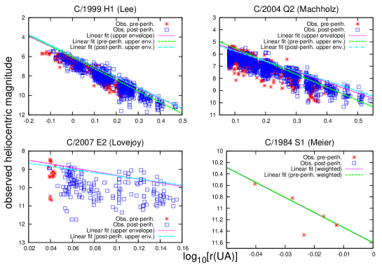
Figure 1: Heliocentric total visual magnitudes as a function of the logarithm of the heliocentric distance, for comets with light curves of different quality classes: C/1999 H1 (Lee) $QC$ = $A$ (upper left panel); C/2004 Q2 (Machholz) $QC$ = $B$ (upper right panel); C/2007 E2 (Lovejoy) $QC$ = $C$ (lower left panel); and C/1984 S1 (Meier) $QC$ = $D$ (lower right panel).

2.3 Comparison between our magnitude estimates and previous ones

As a check to evaluate how our estimated absolute total magnitudes compare with previous determinations, we used a set of comets observed during the 1970s for which we have both, our own estimates and previous ones, essentially from Vsekhsvyatskii, Whipple, Meisel, and Morris (loc. cit.). As we can see in Fig. 2, the mean value of the differences is close to zero, and only four comets (from a sample size of fifteen) present differences larger than 1 $\sigma$ (i.e. differences between about 0.5 and 1.5 magnitudes). We then conclude that our estimates are consistent with those from previous authors, which make us confident that we are not introducing a significant bias in the $H$ estimates, when we combine those from our comet sample for the period 1970-2009 with estimates from other authors for older comet samples.

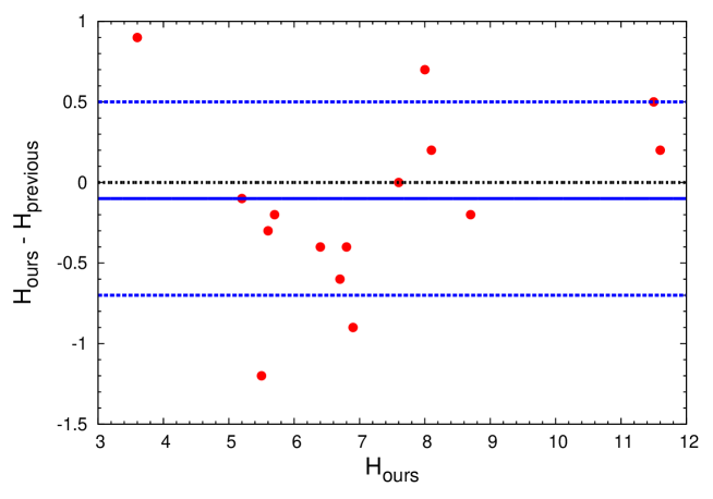
Figure 2: The difference between our estimated absolute total magnitude and previous estimates for a sample of fifteen comets observed between 1970 and 1980, as a function of our estimated magnitudes $H_{ours}$. The horizontal lines represent the mean of the differences, and the mean $\pm$ 1 $\sigma$. The plotted comets are: C/1970 N1, C/1970 U1, C/1971 E1, C/1973 E1, C/1974 C1, C/1975 N1, C/1975 V1-A, C/1975 V2, C/1975 X1, C/1977 R1, C/1978 C1, C/1978 H1, C/1979 M1, C/1980 O1, C/1980 Y1.

3 The discovery rate

We plot in Fig. 3 the discovery year of LPCs with $q<1.3$ AU for the period 1900-2009 versus their absolute total magnitudes. We see that most magnitudes are below $H\simeq 12$, and that this ceiling has changed very little through time despite the systematic sky surveys implemented during the last two decades. By contrast, these surveys have greatly contributed to a dramatic increase in the discovery rate of Near-Earth Asteroids (NEAs) in “cometary” orbits (i.e. with aphelion distances $Q>4.5$ AU) fainter than absolute magnitude 14, with a few as faint as magnitudes 25-30. This is in agreement with the conclusion reached by Francis (2005), who found very few LPCs with $H>11$ from the analysis of a more restricted -but more selected- sample of LPCs discovered by LINEAR that reached perihelion between 2000 January 1 and 2002 December 31.

We also note in Fig. 3 that the density of points for the discovered comets tends to increase somewhat with time. We actually note three regions: the less dense part for the period 1900-1944, an intermediate zone for 1945-1984, and the most dense part for 1985-2009. The fact that the increase has been only very moderate for the last century, and that it has been kept more or less constant for the last 25 years, suggests us that the discovery rate has attained near completion, at least for magnitudes $H\ ^{<}\!\!\!\!_{\sim}\>9$. We have also investigated possible observation selection effects that may have affected, or are still affecting, the discovery rate. We will next analyse this point.

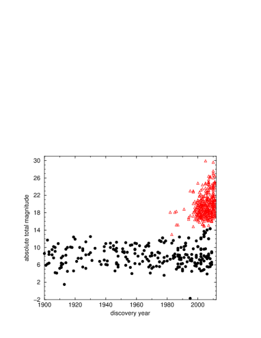
Figure 3: The discovery year versus absolute magnitudes of the sample of 232 LPCs (filled circles) and 375 NEAs in “cometary” orbits (aphelion distances $Q>4.5$ AU) (red triangles). Since NEAs are inactive bodies, “total” means nuclear magnitude in their case.

3.1 The Holetschek effect

The potential discovery of LPCs (i.e. comets that have been recorded only once during the age of scientific observation) is a function of its brightness (which depends on the perihelion distance) and the comet-Earth-Sun geometry. The Holetschek effect is the best known one (e.g. Everhart 1967a, Kresák 1975), and is associated with the fact that comets reaching perihelion on the opposite side of the Sun, as seen from the Earth, are less likely to be discovered. This effect essentially affects comets in Earth-approaching or crossing orbits, as is the case of our sample. In Fig. 4 we show the differences in heliocentric longitude $\Delta l$ between the comet and the Earth computed at the time of the comet’s perihelion passage (the ephemeris data were obtained from JPL Horizon’s orbital integrator). We can see that the Holetschek effect is important for comets observed between 1900 and 1944; it is less important for comets observed between 1945 and 1984, and negligible for comets observed between 1985 and 2009, i.e. when dedicated surveys with CCD detectors began to operate. Hence, we consider the subsample of LPCs observed between 1985 and 2009 as an unbiased sample, at least as regards to this effect.

Figure 4: Distributions of longitude differences $\Delta l=l_{c}-l_{\oplus}$, where $l_{c}$ is the heliocentric longitude of the comet at perihelion, and $l_{\oplus}$ that of the Earth at that time, for the LPC samples for the periods indicated on the panels. To smooth out the histograms, the half portions between 180^∘ and 360^∘ have been folded over the first half portions between 0^∘ and 180^∘. A decrease in the number of comets reaching perihelion near $\Delta l\simeq 180^{\circ}$ is noticed in the two older samples (Holetschek effect).

3.2 The Northern-Southern asymmetry

We have also investigated if it was a dominance of northern discoveries against southern ones. The distribution of the sine of the comet’s declination $\delta$ at discovery does not show a significant drop for high southern declinations ($\delta$ $<$ -30^∘), hence we conclude that the unequal coverage of the northern and southern hemispheres has had little effect on comet discovery, at least for LPCs with $q<1.3$ AU discovered during the last century.

4 The cumulative distribution of absolute visual magnitudes

4.1 The sample of LPCs for the period 1900-2009

In Fig. 5 we present the logarithm of the cumulative number of comets $N_{<H}$ having absolute total visual magnitudes smaller than a specific value $H$, plotted as a function of the absolute magnitude, for the overall comet sample 1900-2009, and for the three sub-samples: 1900-1944, 1945-1984, and 1985-2009. We have normalized the number of discovered comets within the different periods to comets century^-1. We found that within a certain range of $H$, $\log_{10}N_{<H}$ could be well fitted by a linear relation, namely

$$\log_{10}N_{<H}\ =\ \alpha H+C,$$ (3)

where $C$ is a constant, and the slope was found to be $\alpha=0.56\pm 0.10$ for comets with $4.0\leq H<5.8$, and $\alpha=0.20\pm 0.02$ for comets with $5.8\leq H<8.6$, as inferred from what we consider as the most unbiased sub-sample: LPCs for 1985-2009 (see lower left panel of Fig. 5). We note that we used all the observed comets for the period 1985-2009 for deriving the slopes of equation (3), including the most uncertain quality class D. We then checked the previous results by considering only the quality classes A, B and C, leaving aside D-quality comets. We found very minor changes, of a couple of hundredths units in the slopes at most, so we decided to keep the results for the complete sample.

We found similar behaviours for the other sub-samples, namely a steep slope up to $H\sim 6$, and then a smooth slope up to $H\sim 8.6$. Yet, the derived values are somewhat lower: $\alpha\sim 0.35-0.47$ for the first leg, and $\alpha\sim 0.16-0.19$ for the second one, but we should bear in mind that these sub-samples are presumably incomplete, thus affecting the computed values of $\alpha$. We may further argue that because fainter comets are more likely to be missed than brighter ones, the biased cumulative magnitude distributions may be flatter than the real ones, thus explaining the lower values of $\alpha$ computed for the older sub-samples.

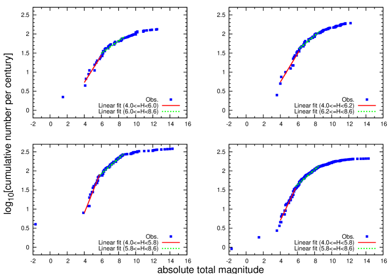
Figure 5: The cumulative distributions of H for the samples: 1900-1944 (upper left panel), 1945-1984 (upper right panel), 1985-2009 (lower left panel), and the overall sample 1900-2009 (lower right panel).

4.2 The ancient comets

An inspection of the overall sample of Fig. 5 (lower right panel) suggests us that the cumulative distribution of comets brighter than $H\simeq 4$ tends to flatten, in other words, it seems to be more bright comets than expected from the extrapolation to brighter magnitudes of the steep slope found for magnitudes $4.0\leq H<5.8$. Unfortunately the number of comets with $H<4$ observed during 1900-2009 is too low to draw firm conclusions. To try to advance in our knowledge of the brighter end of the magnitude distribution, we had to resort to a comet sample observed over a longer time span. We then assembled a sample of LPCs brighter than $H=4.5$ observed during 1500-1900. Our main source was Vsekhsvyatskii’s (1964a) catalogue, complemented with information provided by Kronk and Hasegawa. Even though we may consider the photometric data of ancient comets of lower quality, as compared to those for modern comets, for the time being it is the only source of information available, and we hope from this to gain insight into the question of what is the magnitude distribution of the brighter comets. Fig. 6 shows the discovery rate of LPCs with $q<1.3$ AU brighter than $H=4.5$ discovered over the period 1500-2009. We observe a rather constant flux, at least from about 1650 up to the present (that roughly corresponds to the telescopic era when photometric observations became more rigorous), which suggests that the degree of completeness of the discovery record of bright comets has been very high since then.

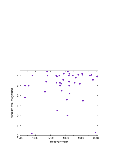
Figure 6: The discovery year versus absolute magnitudes of the sample of 34 ancient LPCs (1500-1899) plus 8 modern LPCs (1900-2009) brighter than $H=4.5$.

Fig. 7 shows the cumulative $H$-distribution of comets brighter than $H=4$. To check how sensitive is the linear fit to small changes in the sample, we tried to fit different sub-samples (as shown in the figure). The samples of Fig. 7 did not include the brightest comet (Hale-Bopp with $H=-1.7$), since its detached position at the brightest end gives it a too strong weight in the computed slope. For the two considered samples: 1650-2009 and 1800-2009, we analised two linear fits: one going up to a magnitude $H=4$, and the other to only $H=3.2$. For $H=4$ we obtained computed slopes 0.32 and 0.26 for the samples 1650-2009 and 1800-2900, respectively, while for $H=3.2$ the respective values decrease somewhat to 0.28 and 0.24, respectively. The slight increase in the computed slope as we pass from a limit at $H=3.2$ to $H=4$ may be explained as due to the approach to the knee found at $H\sim 4$ and the transit to a much steeper slope for fainter comets. We also find that the computed slopes for the most restricted sample 1800-2009 are somewhat higher than the ones obtained for the whole sample 1650-2009, which may de due to the greater incompleteness of the older sample for 1650-1800.

We have also checked the robustness of our computed results by considering two extreme cases: one that includes the brightest comet Hale-Bopp, and the second one that removes the two brightest comets (Hale-Bopp and C/1811 F1 with $H=0$). In the first case we get values for the slope in the range 0.17-0.24; for the second we get values between 0.33-0.38. As a conclusion, from the analysis of different sub-samples, that contemplate different ranges of $H$ and two periods of time, we can derive an average slope aroud 0.28 with an estimated uncertainty $\pm 0.1$.

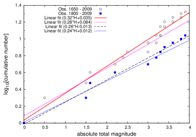
Figure 7: Cumulative distributions of $H$ for several subsets of the brightest comets $H<4$ observed during the period 1650-2009. The brightest comet of the sample, C/1995 O1 (Hale-Bopp), was not taken into account in the linear fits shown here.

4.3 The overall sample

We show in Fig. 8 the concatenated cumulative distributions of $H$ for the sample of bright comets ($H<4$) observed during 1650-2009, and our assumed unbiased sample of LPCs with magnitudes $H\geq 4$ for the period 1985-2009, both linear fits normalized to units of comets century^-1. The concatenated distribution shows three segments: one for the brightest comets ($H<4$) with a slope 0.28, other for those with intermediate brightness ($4\leq H<5.8$) with a slope 0.56, and other for less bright comets ($5.8\leq H<8.6$) with a slope 0.20, as found in Sections 4.2 and 4.1, respectively. The cumulative distribution tends to flatten for comets fainter than $\sim 8.6$, and it levels off for $H\ ^{>}\!\!\!\!_{\sim}\>12$, in agreement with what we said before about the scarcity of LPCs fainter than $H\simeq 12$.

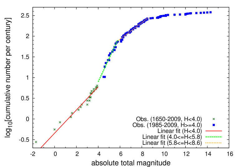
Figure 8: The cumulative distributions of $H$ for the sample of bright comets ($H<4$) observed during the period 1650-2009, and the sample 1985-2009 for comets with $H\geq 4$.

We can convert the cumulative magnitude distribution law: $\log_{10}N_{<H}=C+\alpha H$, into a cumulative size distribution (CSD) law, $N_{>R}$, by means of the relation between the radius $R$ and $H$ given by equation (1). We obtain

$$N_{>R}\ =\ AR^{-s},$$ (4)

where $A$ is a normalization factor, the exponent $s=\alpha/b$, and $b=0.13$ (cf. equation (1)). Likewise, from equation (1) we can convert the magnitude ranges into ranges of $R$, as shown in Table 4. We can also see in the table the values of the parameters $A$ and $s$ obtained for the best-fit solutions. With the $A$ values of Table 4 we obtain cumulative numbers expressed in comets century^-1.

Table 4: Numerical values for the parameters $A$ and $s$ of equation (4)

Range of $R$ (km)	$A$	$s$
$R>2.4$	38.8	$2.15\pm 0.75$
$1.4<R\leq 2.4$	329	$4.31\pm 0.80$
$0.6<R\leq 1.4$	130	$1.54\pm 0.15$

As mentioned in the Introduction, there have been a few attempts before to derive the magnitude distribution of LPCs, and in some cases also their sizes. The knee in the $H$-distribution at $H\simeq 6$ is a well established feature (e.g. Everhart 1967b, Sekanina and Yeomans 1984). From the analysis of the magnitude distribution of LPCs observed during 1830-1978, Donnison (1990) derived a slope $\alpha\simeq 0.34$ for comets with $H<6$. From the study of Vsekhsvyatskii’s sample, Hughes (2001) found a slope $\alpha\simeq 0.36$ within the range $3.5\ ^{<}\!\!\!\!_{\sim}\>H\ ^{<}\!\!\!\!_{\sim}\>6.6$. This corresponds to an exponent $s=2.77$ for the cumulative $R$-distribution, i.e. Hughes obtained something in between our computed values of $\alpha$ and $s$ for our first and second leg ($H<4$ and $4\leq H<5.8$). The problem is that Hughes worked with LPCs of all perihelion distances, thus bringing to his sample distant comets of very uncertain computed values of $H$, and also more affected by observational selection effects.

We can also compare our derived CSD for LPCs with those derived for other populations. Tancredi et al. (2006) derived an exponent $s=2.7\pm 0.3$ for a sample of Jupiter family comets (JFCs) with well determined nuclear magnitudes and $q<2.5$ AU. On the other hand, Lamy et al. (2004) derived a smaller value of $s\simeq 1.9\pm 0.3$. A recent re-evaluation of the CSD of JFCs by Snodgrass et el. (2011) leads to a somewhat greater value of the slope: $s=1.92\pm 0.20$ applicable to comets with radii $\geq$ 1.25 km. The sample of JFCs considered by these authors covered a range of radii from sub-km to several km, i.e. it roughly overlaps part of our first leg of brighter comets, the second and third leg, for which we derived exponents of 2.15, 4.31 and 1.54 respectively.

More light can be shed from theoretical models. For instance, Dohnanyi (1969) derived an exponent $s=2.5$ for a population in collisional equilibrium. Kenyon and Bromley (2012) have considered a protoplanetary disk divided in 64 annuli covering a range of distances to the central star between 15-75 AU. Then the authors simulate the evolution of a swarm of planetesimals distributed among the different annuli in order to follow a predetermined surface density law for the disk. The population goes through a process of coagulation and fragmentation leading to a few oligarchs (large embryo planets), and a large number of small planetesimals that will largely evolve through destructive collisions. What is suggestive for our study is that the authors find an exponent $s=2$ for the CSD of the evolve population that remains in the range $R\sim 10-100$ km, while the exponent is somewhat higher than 2 in the range 1-10 km. Then, Kenyon and Bromley’s (2012) results match very well our computed value of $s=2.15$ for the brighter LPCs with $H<4$ ($R\ ^{>}\!\!\!\!_{\sim}\>2.4$ km). Furthermore, the population of larger comets might precisely be the one that best preserves its primordial size distribution. As we will see below, smaller LPCs may have gone through recent phenomena upon approaching the Sun, as e.g. splitting into two or more pieces, fading into meteoritic dust, that has greatly changed its primordial distribution, as shown in Fig. 8.

5 New comets among the observed LPCs

New comets are usually considered to be those with original energies in the range $0<E_{or}<10^{-4}$ AU^-1, which appear as a spike in the $E_{or}$-histogram of LPCs, as first pointed out by Oort (1950). Since the typical energy change by planetary perturbations is $>>10^{-4}$ AU^-1, these comets are presumably new incomers in the inner planetary region. Admittedly this may not be true in all cases. By integrating the orbits of “new” comets backwards to their previous perihelion passages, considering planetary perturbations and the tidal force of the galactic disk, Dybczyński (2001) found that nearly 50% of the so called new comets actually passed before by the planetary region with $q<15$ AU. From these results he proposed a new definition of new comet based on the condition that the perihelion distance of the previous passage had to be $q_{pre}>15$ AU, thus discarding the criterion based on the original energy. Yet Dybczyński’s definition has its own shortcomings. Firstly, the computed $q_{pre}$ strongly depends on the modeled galactic potential, and on the almost unknown stellar perturbations. Furthermore, the boundary at $q=15$ AU to discriminate between “new” and “old” comets is rather arbitrary. By shifting this value upward or downward we can get different new/old ratios. Therefore, we will stick to the classic definition of new comet based on its original energy, on the dynamical criterion that such a comet comes from the Oort cloud and, thus, has been greatly influenced in its way in by the combined action of galactic tidal forces and passing stars. Evolved comets will then be defined as those with binding energies above $10^{-4}$ AU^-1, so they are no longer influenced by external perturbers. They have already passed before by the inner planetary region (interior to Jupiter’s orbit).

5.1 The observed fraction of new comets in the incoming flux of LPCs

We considered in the first place our sample of LPCs for the period 1900-2009. Unfortunately, reliable computed original energies are available for only a fraction of them. Many comets, mainly those observed prior to about 1980, do not have computed values of $E_{or}$. Therefore, we also analysed the more restricted -though more complete- sample of LPCs brighter than $H=9$ discovered in the last quarter of century (1985-2009). Following other authors (Francis 2005, Neslušan 2007), we also considered more restricted samples from sky surveys that are presumably less biased, and that have computed $E_{or}$ for most of their members. Since our main interest here is to derive the ratio new-to-evolved LPCs, and not so much their absolute magnitudes, for the sky surveys we considered comets covering a much wider range of perihelion distances ($0<q<4$ AU) under the assumption that up to $q\simeq 4$ AU the detection probability was quite high. In short, we analysed the following samples:

• LPCs with $P>10^{3}$ yr and $q<1.3$ AU observed during the period 1900-2009 (232 comets).

• LPCs with $P>10^{3}$ yr, $q<1.3$ AU, and brighter than $H=9$ for the period 1985-2009 (68 comets).

• LPCs with $P>10^{3}$ AU and $q<4$ AU discovered by LINEAR (73 comets).

• LPCs with $P>10^{3}$ AU and $q<4$ AU discovered by other large sky surveys (Siding Spring, NEAT, LONEOS, Spacewatch, Catalina) (45 comets).

The computed original energies were taken from Marsden and Williams’s (2008) catalogue, complemented with some values from Kinoshita and Nakano electronic catalogues (see references in the Introduction). For our comet sample 1900-2009, the values of $E_{or}$ are also included in Tables 2 and 3.

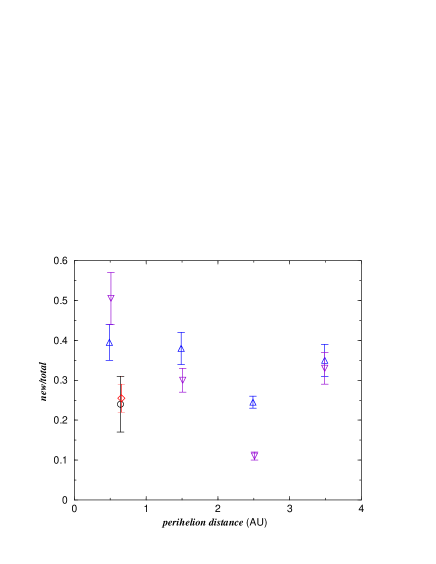
Figure 9: The ratio of new/total LPCs for the different samples as a function of the average perihelion distance of the considered range. The samples are: LPCs observed during the period 1900-2009 with $q<1.3$ AU and all magnitudes (diamond); LPCs observed during 1985-2009 with $q<1.3$ AU and $H<9$ (circle); LINEAR comets with $q<4$ AU discriminated in intervals of 1 AU (triangle down); LPCs from other sky surveys discriminated in intervals of 1 AU (triangle up).

Let $n_{LPC}=n_{new}+n_{ev}$ be the total number of LPCs, comprising both new and evolved LPCs which are given by the quantites $n_{new}$ and $n_{ev}$, respectively. From the $n_{new}/n_{LPC}$ ratios found for the different samples, as shown in Fig. 9, we found as an average

$$\frac{n_{new}}{n_{LPC}}\simeq 0.3\pm 0.1,$$ (5)

or $n_{new}/n_{ev}\sim 0.43$, namely, for about 7 evolved LPCs with $P>10^{3}$ yr we have approximately 3 new comets.

The error bars of the derived values shown in Fig. 9 take into account only the uncertainty within the considered sample due to LPCs of unknown or poorly determined $E_{or}$. However, it does not consider the uncertainty inherent to the finite size $n$ of our samples of random elements (that goes as $n^{1/2}$). How the different error sources play is a complex matter, but we still consider that the uncertainty associated to, or lack of computed values of $E_{or}$, may be the principal one.

5.2 The theoretically expected new/evolved LPCs ratio as a function of the maximum number of passages

Let us assume that we have an initial population of $n_{new}$ comets injected in orbits with $q<1.3$ AU. About half of this population will be lost to the interstellar space, and about half will return as evolved LPCs, in general with bound energies $E>10^{-4}$ AU^-1. After the second passage, these returning comets can either be ejected or come back with a different bound energy, and the same process will repeat again in the following passages. The energies that bound comets get in successive passages can be described as a random walk in the energy space, in which in every passage a given comet receives a kick in its energy due to planetary perturbations. After $N$ passages the number $n_{N}$ that will remain bound to the solar system is (e.g. Fernández 1981, 2005)

$$n_{N}\sim\frac{1}{2}n_{new}N^{-1/2}.$$ (6)

The total number of returns of the $n_{new}$ comets as evolved LPCs, $n_{ev}$, can be computed by summing the returning comets between $N=1$ and a maximum number of passages $N_{max}$ that is set either by the physical lifetime of the comet, or by the dynamical timescale (expressed in number of revolutions) to reach an orbit with $P<10^{3}$ yr (or a binding energy $E>10^{-2}$ AU^-1), namely

$$n_{ev}=\sum^{N_{max}}_{N=1}n_{N}\sim\frac{1}{2}n_{new}\sum^{N_{max}}_{N=1}N^{-1/2}\sim n_{new}N_{max}^{1/2}.$$ (7)

Since $n_{ev}/n_{new}\simeq 7/3$, from equation (7) we find that

$$N_{max}\simeq\left(\frac{n_{ev}}{n_{new}}\right)^{2}\sim 5.5.$$ (8)

This result is in good agreement with that found by Wiegert and Tremaine (1999) from numerical simulations of fictitious Oort cloud comets injected into the planetary region with different fading laws. These authors obtained as the best match to the observed distribution of orbital elements a survival of roughly 6 orbits for the 95% of the comets, while the remainder 5% did not fade. We may argue that this 5% of more robust comets are associated with the largest members of the comet population.

The random walk in the energy space, where each step has a typical change $\Delta E_{t}\sim 10^{-3}$ AU^-1, allows us to estimate the typical number of passages $N_{dyn}$ required to reach an energy $E>E_{L}=10^{-2}$ AU^-1 (or a period $P<10^{3}$ yr)

$$N_{dyn}\sim\left(\frac{E_{L}}{\Delta E_{t}}\right)^{2}=10^{2}.$$ (9)

We find that $N_{max}<<N_{dyn}$, i.e. most comets will be destroyed by physical processes (sublimation, outbursts, splittings) before reaching energies $>E_{L}$.

5.3 Comets coming from the outer and from the inner Oort cloud

Among the new comets, we distinguish in turn those coming form the outer Oort cloud, with energies in the range $0<E_{or}<0.3$, from those coming from the inner Oort cloud, with energies in the range $0.3\leq E_{or}<1$ (both in units of $10^{-4}$ AU^-1). Outer Oort cloud comets (semimajor axis $a\ ^{>}\!\!\!\!_{\sim}\>3.3\times 10^{4}$ AU) can be driven from the outer planetary region to the inner planetary region in a single revolution by the combined action of galactic tidal forces and passing stars, so they can overshoot the powerful Jupiter-Saturn gravitational barrier (e.g. Fernández 2005, Rickman et al. 2008). On the contrary, the stronger gravitationally bound comets in the inner Oort cloud will require more than one revolution to diffuse their perihelia to the inner planetary region, so they will meet in their way in the Jupiter-Saturn barrier, with the result that most of the comets will be ejected before reaching the near-Earth region. From the study of the discovery conditions of a sample of 58 new comets discovered during 1999-2007, Fernández (2009) found that comets in the energy range $0<E_{or}(10^{-4}\mbox{ AU${}^{-1}$})<0.3$ show a uniform $q$-distribution, as expected from comets injected straight into the inner planetary region from a thermalised population, while the $q$-distribution of comets with original energies $0.3<E_{or}(10^{-4}\mbox{ AU${}^{-1}$})<1$ show an increase with $q$ which may be attributed to the Jupiter-Saturn barrier that prevents most of the inner Oort cloud comets from reaching the inner planetary region. As a corollary, we infer that the ratio outer-to-inner Oort cloud comets derived for the Earth neighbourhood should decrease when we consider new comets beyond Jupiter.

We note than when we talk about comets coming from a given region, we mean the region attained during the last orbit. As shown by Kaib and Quinn (2009), a comet from the inner Oort cloud whose perihelion approaches the Jupiter-Saturn barrier can receive a kick in its energy that sends it to the outer Oort cloud where the stronger galactic tidal forces and stellar perturbations can deflect it to the near-Earth region, overcoming in this way the Jupiter-Saturn barrier. Therefore, we cannot tell for sure if a comet has resided for a long time in the outer or inner Oort cloud, but only the place from where it comes in the observed apparition. It is very likely that Kaib and Quinn’s mechanism provides a steady leaking of comets from the inner to the outer Oort cloud.

The estimate of the ratio outer-to-inner is a very complex matter since we are dealing with very narrow energy ranges ($\Delta E\simeq 0.3\times 10^{-4}$ AU^-1 for the outer Oort cloud, and $\Delta E\simeq 0.7\times 10^{-4}$ AU^-1 for the inner Oort cloud), so the errors in the computation of original orbital energies may be of the order of these ranges. Even though the formal errors of the computed original orbital energies of comets of quality classes 1A and 1B in Marsden and Williams’s (2008) catalogue are $\pm 5$ and $\pm 12$ (in units of $10^{-6}$ AU^-1), respectively, unaccounted nongravitational (NG) effects may shift the computed $E_{or}$ by several tens of units, as shown by Królikowska and Dybczyński (2010). We will neglect NG forces for the moment, and come back to this complex issue below. In Table 5 we show the outer-to-inner ratio of QC 1A comets. We consider three ranges of perihelion distances: $0<q\leq 1.5$ AU, $1.5<q\leq 3.0$ AU, $3.0<q\leq 4.5$ AU. The available samples are very likely incomplete, though we hope that the incompleteness factor is similar for comets from the inner and from the outer Oort cloud, so the ratio will remain more or less constant.

Table 5: Ratio of comets coming from the outer Oort cloud to those coming from the inner Oort cloud.

$\Delta q$	Outer : Inner
$0<q\leq 1.5$	7 : 5
$1.5<q\leq 3$	10 : 8
$3<q\leq 4.5$	13 : 18

There is a slight predominance of new comets coming from the outer Oort cloud than from the inner Oort cloud in the first two $q$ ranges. In the most distant one the situation reverses and there are more comets coming from the inner Oort cloud. As said above, the outer-to-inner ratio does not have to keep constant throughout the planetary region. On the contrary, as $q$ increases it is expected that more comets from the inner Oort cloud will be present as we pass over and leave behind the Jupiter-Saturn barrier. We have also checked the outer-to-inner ratios for the sample of QC 1B comets despite their lower quality. We find 9:9, 6:6 and 1:4 for the ranges $0<q\leq 1.5$ AU, $1.5<q\leq 3$ AU, and $3<q\leq 4.5$ AU, respectively. The trend remains more or less the same: we may argue that the slight decrease in the outer-to-inner ratios from 1A to 1B comets for the first two ranges, $0<q\leq 1.5$ AU and $1.5<q\leq 3$ AU, is due to some blurring in the computed original orbit energies of the lower quality class 1B comets. If there is some reshuffling, it will be more likely that errors will put an outer Oort Cloud comet in the energy range of inner Oort Cloud comets than the other way around, simply because the width of the inner Oort Cloud energy range is more than twice that of the outer Oort Cloud.

Let us call $n_{in}$ and $n_{out}$ the number of new comets coming from the inner and outer Oort cloud, respectively, such that $n_{new}=n_{in}+n_{out}$. From the previous analysis, we find that $n_{out}$ may be a little above $n_{in}$ in the zone closer to the Sun (say $q\ ^{<}\!\!\!\!_{\sim}\>3-4$ AU) with an error bar that may leave the lower end slightly below one, so we can estimate

$$\frac{n_{out}}{n_{in}}\simeq 1.1\pm 0.2$$ (10)

Let us now come back to the problem of unaccounted NG forces that might affect the $E_{or}$ values computed by Marsden and Williams (2008). Królikowska and Dybczyński (2010) and Dybczyński and Królikowska (2011) have recomputed the orbits of “new” comets, as defined by Marsden and Williams, including NG terms in the equations of motion. The authors find that the inclusion of NG forces tends to shift the computed $E_{or}$ to greater values (smaller semimajor axes). This shift could affect the computed ratio $n_{out}/n_{in}$, as some comets will move from original hyperbolic orbits to the Oort cloud, and others from the Oort cloud to evolved orbits. Królikowska and Dybczyński (2010) computed original orbits of comets with $E_{or}<10^{-4}$ AU^-1 and $q<3$ AU, whereas Dybczyński and Królikowska (2011) considered those with $q>3$ AU. While the orbits computed with NG forces were the best for the first case, for comets with $q>3$ AU only 15 out of 64 comets presented measurable NG forces. Altogether, they assembled a sample of 62 comets whose computed original energies (mostly NG solutions) fall in the range $0<E_{or}<10^{-4}$ AU^-1. From these computed set of energies, we find that 26 comets come from the outer Oort cloud ($E_{or}<0.3\times 10^{-4}$ AU^-1), and 36 from the inner Oort cloud. If we limit the sample to comets with $q>3$ AU, less affected by NG forces, the numbers are: 20 from the outer Oort cloud and 18 from the inner Oort cloud, i.e. an $n_{out}/n_{in}$ ratio slightly above unity. If we now extrapolate this result to smaller $q$, we should expect a slight increase of this ratio (see discussion above), though still compatible with the one shown in equation (10).

6 Evolutive changes in the size distribution: sublimation and splitting

Comet splitting is a rather common phenomenon observed in comets (e.g. Chen and Jewitt 1994). In most cases small chunks and debris are released of very short lifetime, so the process can be described as a strong erosion of the comet nucleus surface, but essentially it remains as a single body. Yet, in some occasions the splitting of the parent comet may lead to two or more massive fragments that become unbound, and may last for several revolutions, thus producing daughter comets that may be discovered as independent comets. We have several cases of comet pairs among the observed LPCs which are shown in Table 6. We include in the table only those comets whose splittings are attributed to endogenous causes, namely we are leaving aside comets that tidally split in close encounters with the Sun or planets.

Table 6: LPC pairs.

Pair	$q$ (AU)
1988 F1 Levy and 1988 J1 Shoemaker-Holt	1.17
1988 A1 Liller and 1996 Q1 Tabur	0.84
2002 A1 LINEAR and 2002 A2 LINEAR	4.71
2002 Q2 LINEAR and 2002 Q3 LINEAR	1.31

The splitting phenomenon is a consequence of the very fragile nature of the comet material. For instance, from the tidal breakup of comet D/1993 F2 (Shoemaker-Levy 9) in a string of fragments, Asphaug and Benz (1996) found that the tidal event could be well modeled by assuming that the nucleus was a strengthless aggregate of grains. The high altitudes at which fireballs (of probable cometary origin) are observed to disrupt also lead to low strengths between $\sim 10^{3}$ - $10^{5}$ or $10^{6}$ erg cm^-3 (Ceplecha and McCrosky 1976; Wetherill and ReVelle 1982). Also from the analysis of the height of meteoroid fragmentation, Trigo-Rodríguez and Llorca (2006) find that cometary meteoroids have typical strengths of $\sim 10^{4}$ erg cm^-3, though it is found to be of only $\sim 4\times 10^{2}$ erg cm^-3 for the extremely fluffy particles released from 21P/Giacobini-Zinner.

Samarasinha (2001) has proposed an interesting model to explain the breakup of small comets like C/1999 S4 (LINEAR). The author assumes a rubble-pile model for the comet nucleus with a network of interconnected voids. The input energy comes from the Sun. The solar energy penetrates by conduction raising the temperature of the outer layers of the nucleus. As the heat wave penetrates, an exothermic phase transition of amorphous ice into cubic ice may occur when a temperature of 136.8 K is attained, releasing an energy of $8.4\times 10^{8}$ erg g^-1 (Prialnik and Bar-Nun 1987). The released energy can go into the sublimation of some water ice and the liberation of the CO molecules, trapped in the ice matrix, that propagate within the network filling the voids, thus building a nucleus-wide gas pressure able to disrupt a weakly consolidated body. As the self-gravity scales as $R^{2}$, larger comet nuclei might be able to hold the fragments together. Therefore, we may infer that there is a critical radius below which the breakup with dispersion of fragments occurs, since the self-gravity is too weak to reassemble the fragments.

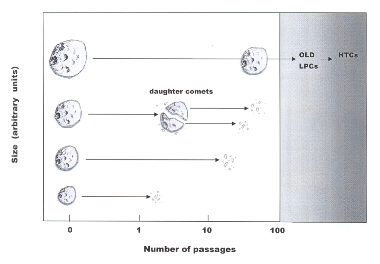
Figure 10: Sketch depicting the physical evolution of nuclei of different sizes.

Fig. 10 depicts possible physical pathways for comets of different sizes that summarize what we have discussed in this paper. Large comets (about ten-km size or larger) can survive for hundreds or thousands of revolutions so they may reach old dynamical ages (Halley types). Large comets are essentially lost by hyperbolic ejection. Medium-size comets (several km) does not have enough gravity field to avoid the separation of fragments upon breakups which may lead to the production of daughter comets that continue their independent lives until disintegration or ejection. Small comets (about one km) can last several passages until disintegration without producing daughter comets (namely fragments are too small to last for long enough to be detected as independent comets). Finally, very small comets (some tenths km) quickly disintegrate after one or a few passages at most.

7 A numerical model

We developed a simple model to simulate the dynamical and physical evolution of cometary nuclei of different sizes entering in the inner Solar System from the Oort Cloud. Our aim was to try to reproduce, in a qualitative sense and broad terms, the observed size distribution (as inferred from the absolute magnitude distribution of the observed LPCs shown in Fig. 8). We performed numerical simulations for large samples of fictitious comets with initial parabolic orbits (original orbital energies $E=0$), random inclinations, and a perihelion distance $q=1$ AU, varying the nuclear radius from 0.5 km up to 50 km, with a size bin of 0.25 km, so we considered 198 initial radii. For every initial radius, we computed samples of $10^{4}$ fictitious comets, so we studied a total of $198\times 10^{4}$ comets for each one of the runs (that have associated the sets of initial conditions shown in Table 7). In every passage of a test comet by the planetary region, we compute the orbital energy change $\Delta E$ due to planetary perturbations. The perihelion distance and the angular orbital elements were assumed to remain constant through the simulation, as they are little affected by planetary perturbations. We assumed that $\Delta E$ followed a random Gaussian distribution (e.g. Fernández 1981), with a mean value = 0 and a standard deviation $\sigma_{E}=7\times 10^{-4}$ AU^-1. We note that the only purpose for assuming a “random inclination” for the comet’s orbit is to adopt an inclination-averaged value of $\sigma_{E}$. The simulations were terminated when the test comets reached one of the following end states:

• they became periodic, i.e. they reached an orbital energy $\geq 10^{-2}$ AU^-1, corresponding to a orbital period $P\leq 10^{3}$ yr;

• they were ejected from the Solar System, i.e. they reached (in our convention of sign) a negative orbital energy;

• they were disintegrated after several passages due to sublimation, i.e reached a radius below a certain minimum radius $R_{min}=0.25$ km; or

• they reached a maximum number of 2000 orbital revolutions.

The following model parameters were allowed to change in each simulation:

• the radius decrease $\Delta R$ per perihelion passage, due to sublimation and other related effects, as for instance outbursts and release of chunks of material from the surface. We adopted for the radius decrease the following expression: $\Delta R=\lambda\Delta R_{s}$, where $\lambda$ is a dimensionless factor, and $\Delta R_{s}$ is the decrease in the radius due to sublimation of water ice, which for a nucleus of bulk density $\rho$ is given by

  $$\Delta R_{s}=\frac{\Delta m_{s}}{\rho},$$ (11)

  where $\Delta m_{s}$ is the mass loss per unit area due to sublimation. This quantity can be computed from the polynomial fit by Di Sisto et al. (2009) to theoretical thermodynamical models of a free-sublimating comet nucleus

  $$\Delta m_{s}\approx 1074.99-4170.89q+8296.96q^{2}-8791.78q^{3}+4988.9q^{4}-1431.4q^{5}+162.975q^{6},$$ (12)

  where $q$ is given in AU and $\Delta m_{s}$ in g cm^-2. We solve equation (12) for $q=1$ AU, that was our adopted perihelion distance for the test comets, and took $\rho=0.4$ g cm^-3 for computing $\Delta R_{s}$ from equation (11).

• a lower and an upper limit radii ($R_{sp1}$ and $R_{sp2}$, respectively) for the occurrence of splitting leading to the creation of two daughter comets. In other words, if the comet reached a radius within the range [$R_{sp1}$ $R_{sp2}$], it was allowed to split in a pair of comets of a half the mass of the parent comet each, with a certain frequency $f_{sp}$.

• the frequency of splittings $f_{sp}$.

In some simulations, we added a few more parameters: an intermediate critical radius $R_{spi}$, between $R_{sp1}$ and $R_{sp2}$, and two frequencies “high” and “low”, $f_{sph}$ and $f_{spl}$, respectively, instead of $f_{sp}$. Under these conditions, comets with radii $R_{sp1}<R<R_{spi}$ were allowed to split with a frequency $f_{sph}$, and comets with $R_{spi}<R<R_{sp2}$ with a frequency $f_{spl}$.

We show in Table 7 the initial conditions chosen for our four runs of $198\times 10^{4}$ fictitious comets each.

Table 7: Initial conditions

Run	$\Delta R$	$\lambda$	$R_{sp1}$	$R_{spi}$	$R_{sp2}$	$f_{sp}$	$f_{sph}$	$f_{spl}$
	(km)		(km)	(km)	(km)
1	0.025	7.7	1.6	-	2.7	0.1	-	-
2	0.025	7.7	1.8	-	5.0	0.05	-	-
3	0.0125	3.9	1.8	3.4	5.0	-	0.1	0.05
4	0.00625	1.9	1.8	3.4	5.0	-	0.1	0.05

Fig. 11 illustrates the physico-dynamical evolution of one of our samples of $10^{4}$ comets with an initial radius $R=6$ km taken from Run 2. All the comets are injected in parabolic orbits ($E=0$) (lower right corner of the panel). The survivors return in orbits of different bound energies $E$ and decreasing radii $R$ due to erosion. The evolution can be seen as a diffusion in the parametric plane $(R,E)$. The different colours represent the different number of passages with a given combination of $R$ and $E$. As the comets get dynamically older (a greater average number of passages), their radii decrease by erosion. This is the reason why the diffusion proceeds from the lower right corner to the upper left side of the diagram.

When the model comets decreased their radii below $R_{sp2}=5$ km, they were allowed to split in two daughter comets with a frequency of one every 20 passages. The splitting event is random, so this was simulated by picking a random number $z$ within the interval $(0,1)$, and imposing the condition that the splitting occurred if $z<0.05$. The production of daughter comets gives rise to a second wave of comet passages toward the left-hand side of the diagram. Comets that reached radii below $R_{sp1}=1.8$ km were assumed to proceed to disintegration without producing daughter comets.

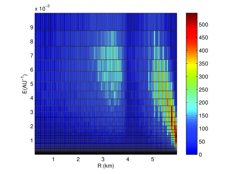
Figure 11: Physico-dynamical evolution of a sample of $10^{4}$ fictitious comets starting in parabolic orbits of radius $R=6$ km taken from the Run 2. The two diffusion zones correspond to the parent and daughter comets. The different colours indicate different number densities of passages with given sets ($R$,$E$).

Once we computed the 198 samples of different initial radii $R_{i}$ of a given run, we assembled the $R_{i}$ samples into a single comet population. We next tried to match the differential $R$-distribution of this population to an assumed differential radius distribution $n_{R}=dN_{R}/dR\propto R^{-\nu}$, where we adopted $\nu=s+1=3.15$, namely the same index as that derived for the largest comets (cf. Section 4.3), that we assumed for our model as the representative of the Oort cloud population. In other words, we assume that the largest observed LPCs have been preserved almost unscathed since their injection into the inner planetary region, so their observed CSD reflects that of Oort cloud comets, and that it extends to smaller comets in the Oort cloud, down to the smallest radius considered in our model. Since all the samples have $10^{4}$ comets (and thus provide an uniform differential $R$-distribution), we transformed it to an $R$-distribution $\propto R^{-\nu}$ just by multiplying a given sample of radius $R_{i}$ by the scaling factor $R_{i}^{-\nu}$. By adding the different samples of $R_{i}$, scaled by $R_{i}^{-\nu}$, we can obtain the cumulative distribution for the sample of new + evolved comets.

Fig. 12 shows the cumulative distribution of the nuclear radius (evolved as well as new comets), with both axes in logarithmic scales, corresponding to the Run 2. The model parameter values for this simulation were: $\Delta R=0.025$ km ($\lambda\simeq 7.7$), $f_{sp}$ = 1/20, $R_{sp1}=1.8$ km, and $R_{sp2}=5.0$ km. A size bin of 0.025 km was used. We can see that the slope of the largest comets $=+2.3$ is not very different from the primordial one ($+2.15$). Yet, in the region where daughter comets are created the slope raises to $+3.3$. The model slope is still lower than the one derived before ($+4.31$) for the range of radii between 1.4 - 2.4 km, which suggests that splitting may not be the only cause for the change of slope at $H\sim 4$, and that other cause (primordial?) may add to the previous one. We obtained a ratio $n_{new}$/$n_{LPC}=0.22$ for this simulation. The computed ratio is still lower than the observed one (0.30, cf. equation (5)), which suggests that we still require higher erosion rates per orbital revolution: $\Delta R>0.025$ km, or $\lambda>7.7$, to match the observed ratio $n_{new}/n_{LPC}$. This ratio decreased to about 0.07 for comets with radii $R>2.75$ km, which is to be expected since large comets have very likely longer physical lifetimes, thus yielding more passages as evolved comets per new comet.

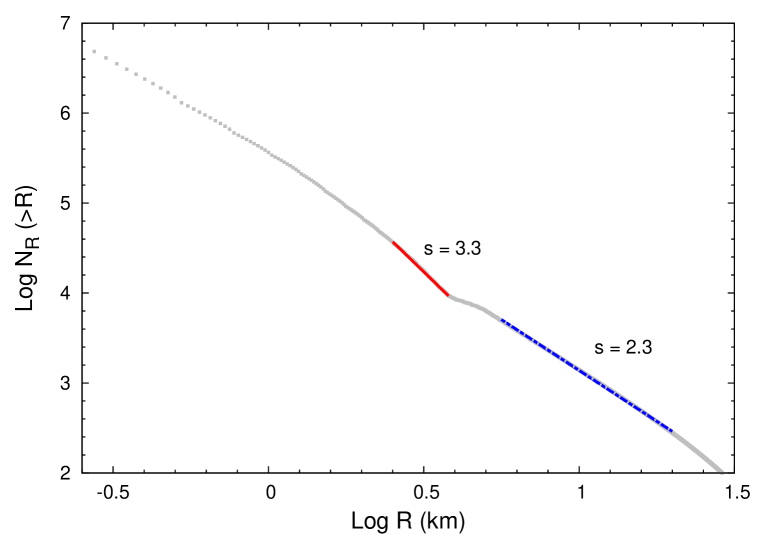
Figure 12: Computed cumulative size-distribution of a sample of $198\times 10^{4}$ fictitious comets of Run 2.

As expected, the match between the computed and the observed ratios $n_{new}$/$n_{LPC}$ worsened when we considered lower erosion rates. We obtained $n_{new}$/$n_{LPC}$ = 0.16 when we changed to $\Delta R=0.0125$ km ($\lambda\simeq 3.9$), while the slopes remain almost unchanged. For $\Delta R=0.00625$ km ($\lambda\simeq 1.9$), $R_{sp1}$ = 1.8 km, $R_{spi}$ = 3.4 km, $f_{sph}$ = 0.1, and $f_{sl}$ = 0.05, we obtained $n_{new}$/$n_{LPC}$ = 0.12, again with slopes close to -3.3 and -2.3. As seen, the results for the cumulative $R$-distribution are quite robust, almost independent of the adopted erosion rate. On the other hand, the differences in the computed ratio $n_{new}$/$n_{LPC}$ are quite substantial from run to run.

8 Summary and conclusions

The most important results of our work can be summarised in the following points:

1. We have ellaborated an updated catalogue of absolute total visual magnitudes $H$ for the LPCs with $q<1.3$ AU observed during 1970-2009.

2. We have analysed the cumulative distribution of $H$, finding at least a three-modal distribution with slopes $\alpha\simeq 0.28\pm 0.10$ for the brightest comets with $H<4$, $\alpha\simeq 0.56\pm 0.10$ for comets with intermediate brightness ($4\leq H<5.8$), and $\alpha\simeq 0.20\pm 0.02$ for the fainter comets ($5.8\leq H<8.6$). From the relation between $H$ and the radius $R$ (cf. equation (1)), we can derive the cumulative size distribution, which can be expressed by a power-law: $N_{>R}=AR^{-s}$, where $s\simeq+2.15$ for $R\ ^{>}\!\!\!\!_{\sim}\>2.4$ km, $s\simeq+4.31$ for $1.4\ ^{<}\!\!\!\!_{\sim}\>R\ ^{<}\!\!\!\!_{\sim}\>2.4$ km, and $s\simeq+1.54$ for $0.6\ ^{<}\!\!\!\!_{\sim}\>R\ ^{<}\!\!\!\!_{\sim}\>1.4$ km.

3. The change at $H\sim 4$ from a rather shallow slope to a steep one may be at least partially explained as a result of splitting and separation of the fragments, thus leading to the creation of two or more daughter comets. Comets brighter than $H\sim 4$ may as well split but their gravitational fields are strong enough to keep the fragments bound.

4. Comets fainter than $H\sim 5.8$ may be too small to survive for more than one or a few passages, so parent comets as well as their daughters might go through a fast fading process, thus explaining the flattening of the cumulative $H$-distribution.

5. The cumulative $H$-distribution flattens even more for LPCs fainter than $H\simeq 8.6$, reaching a ceiling at $H\sim 12$ (diameter $\sim 0.5$ km). We suggest that the scarcity of extremely faint LPCs is a real phenomenon, and not due to observational selection effects. This is supported by several sky surveys which have been very successful at discovering a large number of very faint NEAs (absolute magnitudes $\sim 14-25$) in cometary orbits, but failed to discover a significant number of faint LPCs.

6. The fraction of new comets within the LPC population with $q<1.3$ AU is found to be $0.3\pm 0.1$, namely we have about 3 new comets for every 7 evolved ones. This implies that the average number of returns of a new comet coming within 1.3 AU from the Sun is about 2.3.

7. The ratio between new comets coming from the outer Oort cloud to those coming from the inner Oort cloud, within 1.3 AU from the Sun, is found to be: $1.1\pm 0.02$.

8. We have simulated the physical and dynamical evolution of LPCs by means of a simple numerical model. We find that erosion rates greater than about 8 times the free sublimation rate of water ice are required to match the observed new-to-evolved LPCs ratio. With a splitting rate of one every 20 revolutions, we find an increase in the slope for intermediate brightness comets from 2.3 to 3.3. Even though there is an agreement in qualitative terms, the computed increase in the slope falls short of reproducing the observed slope: 4.31 for comets of this size range. Therefore, other effects might be at work to explain such an increase as, for instance, primordial causes (namely related to the accretion processes and collisional evolution), or the production of multiple fragments that might survive several revolutions as independent comets. As suggested by Stern and Weissman (2001), the scattering of cometesimals by the Jovian planets to the Oort cloud was preceded by an intense collision process between cometesimals and their debris. This process could have led to a heavily fragmented population of comets, just in the size range of a few km. Comets with radii $R\ ^{>}\!\!\!\!_{\sim}\>5-10$ km could have suffered catastrophic collisions, but their gravitational fields were powerful enough to reaccumulate the majority of their fragments, thus preserving their primordial size distribution, though with an internal structure like a ’rubble pile’ (e.g. Weissman 1986). If the initial comet population with radii in the range $\sim 1-10$ km was collisionally relaxed, then the slope of the CSD was close to $s=2.5$ (e.g. Dohnanyi 1969, Farinella and Davis 1996). Yet, since bodies with $R\ ^{>}\!\!\!\!_{\sim}\>$ a few km reaccumulated their fragments, the primordial CSD of slope $s\simeq 2.15$ might have been preserved, thus reflecting the coagulation/fragmentation conditions in the early protoplanetary disk (Kenyon and Bromley 2012). Therefore we might argue that when the scattered cometesimals reached the Oort cloud, they already had a bimodal size distribution. Breakups into daughter comets during passages into the inner planetary region might only enhance an already existing bimodality in the size distribution. No doubt, this is a point that deserves further study.

ACKNOWLEDGMENTS

We want to thank Daniel Green for providing us data in electronic form from the ICQ archive. We also thank Ramon Brasser and the referee, Hans Rickman, for their comments and criticisms on an earlier version of the manuscript that greatly helped to improve the presentation of the results. AS acknowledges the national research agency, Agencia Nacional de Investigación e Innovación, and the Comisión Sectorial de Investigación Científica, Universidad de la República, for their financial support for this work, which is part of her PhD thesis at the Universidad de la República, Uruguay.

References

- [1]
- [2] Asphaug E., and Benz W., 1996, Icarus, 121, 225.
- [3] Chen J., and Jewitt D., 1994, Icarus, 108, 265.
- [4] Dybczyński P.A., 2001, A&A, 375, 643.
- [5] Dybczyński P.A., and Królikowska M., 2011, MNRAS, 416, 51.
- [6] Di Sisto R.P., Fernández J.A., and Brunini A., 2009, Icarus, 203, 140.
- [7] Dohnanyi J.S., 1969, J. Geophys. Res. 74, 2531.
- [8] Donnison J.R., 1990, MNRAS 245, 658.
- [9] Everhart E., 1967a, AJ, 72, 716.
- [10] Everhart E., 1967b, AJ, 72, 1002.
- [11] Farinella P. and Davis D.R., 1996, Sci., 273, 938.
- [12] Fernández J.A., 1981, A&A, 96, 26.
- [13] Fernández J.A., 2005, Comets - Nature, Dynamics, Origin, and their Cosmogonical Relevance. Springer-Verlag.
- [14] Fernández J.A., 2009, in Fernández J.A., Lazzaro D., Prialnik D., Schulz R., eds., Icy Bodies of the Solar System, IAU Symp 263, Cambridge Univ. Press, Cambridge, p.76.
- [15] Francis P.J., 2005, ApJ 635, 1348.
- [16] Green D.W.E., 2010, International Comet Q. archive of photometric data on comets in electronic form, Smithsonian Astrophysical Observatory, Cambridge, MA.
- [17] Hasegawa I., 1980, Vistas in Astronomy, 24, 59.
- [18] Hughes D.W., 1988, Icarus, 73, 149.
- [19] Hughes D.W., 2001, MNRAS, 326, 515.
- [20] Jenniskens P., 2008, Earth, Moon, Planets, 102, 505.
- [21] Kaib N.A., and Quinn T., 2009, Sci., 325, 1234.
- [22] Kenyon S.J., and Bromley B.C., 2012, AJ, 143, 63.
- [23] Kresák L., 1975, Bull. Astron. Inst. Czech., 26, 92.
- [24] Kresák L., and Pittich E.M., 1978, Bull. Astron. Inst. Czech., 29, 299.
- [25] Królikowska M., and Dybczyński P. A., 2010, MNRAS, 404, 1886.
- [26] Kronk G.W., 1999, Cometography. A Catalog of Comets. Ancient-1799. Volume 1. Cambridge Univ. Press, Cambridge.
- [27] Kronk G.W., 2003, Cometography. A Catalog of Comets (1800-1899). Volume 2. Cambridge Univ. Press, Cambridge.
- [28] Lamy P.L., Toth I., Fernández Y.R., and Weaver H.A., 2004, in Festou M., Keller H.U., Weaver H.A., eds., Comets II, Univ. Arizona Press, Tucson, p.223.
- [29] Marsden B.G., and Williams G.V., 2008, 17th. Catalogue of Cometary Orbits. Smithsonian Astrophysical Observatory, Cambridge, MA.
- [30] Meisel D.D., and Morris C.S., 1976, in Donn B., Mumma M., Jackson W., A’Hearn M., Harrington R., eds., The Study of Comets Part 1, NASA SP-393, Washington D.C., p.410.
- [31] Mattiazzo M., 2011, IAU Circ.9226.
- [32] Meisel D.D., and Morris C.S., 1982, in Wilkening, ed., Comets, Univ. Arizona Press, Tucson, p.413.
- [33] Neslušan L., 2007, A&A, 461, 741.
- [34] Oort J.H., 1950, Bull. Astr. Inst. Neth., 11, 91.
- [35] Prialnik D., and Bar-Num A., 1987, ApJ, 313, 893.
- [36] Rickman H., Fouchard M., Froeschlé C., and Valsecchi G.V., 2008, Cel. Mech. Dyn. Astr., 102, 111.
- [37] Samarasinha N.H., 2001, Icarus, 154, 540.
- [38] Sekanina Z., 1997, A&A, 318, L5.
- [39] Sekanina Z., Tichý M., Tichá J., and Kočer M., 2005, Int. Comet Q., 27, 141.
- [40] Sekanina Z., and Yeomans D.K., 1984, AJ, 89, 154.
- [41] Snodgrass C., Fitzsimmons A., Lowry S.C., and Weissman P.R., 2011, MNRAS, 414, 458.
- [42] Sosa A., and Fernández J.A., 2009, MNRAS, 393, 192.
- [43] Sosa A., and Fernández J.A., 2011, MNRAS, 416, 767.
- [44] Stern S.A., and Weissman P.R., 2001, Nat., 409, 589.
- [45] Szabó Gy.M., Sárneczky K., and Kiss L.L., 2011, A&A, 531, A11.
- [46] Tancredi G., Fernández J.A., Rickman H., and Licandro J., 2006, Icarus 182, 527.
- [47] Trigo-Rodríguez J.M., and Llorca J., 2006, MNRAS 372, 655.
- [48] Vsekhsvyatskii S.K., 1963, Sov. Astr., 6, 849.
- [49] Vsekhsvyatskii S.K., 1964a, Physical Characteristics of Comets. Israel Program for Scientific Translation Ltd. Jerusalem.
- [50] Vsekhsvyatskii S.K., 1964b, Sov. Astr., 8, 429.
- [51] Vsekhsvyatskii S.K., 1967, Sov. Astr., 10, 1034.
- [52] Vsekhsvyatskii S.K., and Il’ichishina N.I., 1971, Sov. Astr., 15, 310.
- [53] Weissman P.R., 1986, Nat., 320, 242.
- [54] Whipple F.L., 1978, Earth, Moon, Planets, 18, 343.
- [55] Wiegert P., and Tremaine S., 1999, Icarus, 137, 84.