Master equation for cascade quantum channels: a collisional approach

Abstract

It has been recently shown that collisional models can be used to derive a general form for the master equations which describe the reduced time evolution of a composite multipartite quantum system, whose components “propagate” in an environmental medium which induces correlations among them via a cascade mechanism. Here we analyze the fundamental assumptions of this approach showing how some of them can be lifted when passing into a proper interaction picture representation.

1 Introduction

In the study of the open dynamics of a multipartite quantum system it is frequently made the simplifying assumption that each subsystem interacts with its own local environment. In the language of quantum communication [1] this is equivalent to saying that the resulting time evolution is memoryless i.e. that the noise tampering the communication acts independently on each local component (information carrier) of the transmitted quantum message. In recent years, however, it has been shown that interesting new features emerge when one makes the realistic assumption that the action of a channel over consecutive uses is correlated [2, 3, 4, 5, 6, 7, 8]. Such correlations have been phenomenologically described in terms of a Markov chain which gives the joint probability distribution of the local Kraus operators acting on the individual carriers [2]. Alternatively they have been effectively represented in terms of local interactions of the carriers with a common multipartite environment which is originally prepared into a correlated (possibly entangled) initial state [6], or with a structured environment composed by local and global components [3, 4, 5]. These models, although physically well motivated do not have an intrinsic time structure, in other words they are unable to describe a situation in which the information carriers interact one after the other with an environment which in the meanwhile evolves. For instance consider the case in which an ordered sequence of spatially separated photon pulses carrying information in their photon number, propagates at constant speed in a non passive, lossy optical fiber characterized by (relatively) slow reaction times. If the speed of the pulses is sufficiently high, one might expect that, thanks to the mediation of the fiber, excitations from one pulse could be passed to the next one modifying their internal states via a (partially incoherent) cascade mechanism (see Fig. 1 a) for a schematic representation of the process). The net result of course is the creation of delocalized excitations over the whole string of carriers as they proceed along the fiber (the extent of such delocalization depending upon the ratio between the transmission rate at which the carriers are fed into the fiber and the dissipation rate of the latter). Alternatively, consider the case in which a linear array of local quantum systems (say a set of driven QED cavities as in Fig. 1 b), or a set of quantum dots composing a quantum cascade laser [9]), are indirectly coupled via unidirectional environmental mediators (the photons emitted by the cavities or by the dots) which passing from one system to the other, allow them to exchange excitations  [10, 11, 12, 13, 14, 15, 16]. As in the previous case, the formation of delocalized excitations is expected as time passes (in this case the delocalization of the excitation will depend upon the product between the damping rate of the mediator and the distance between two consecutive quantum systems).

The general form for master equations which describe these situations has been recently derived in Ref. [17] by adopting a collisional approach [18, 19] to describe the system/environment coupling. We aim to review these findings, focusing on some technical aspects of the problem which allows us to lift some of the assumptions of Ref. [17].

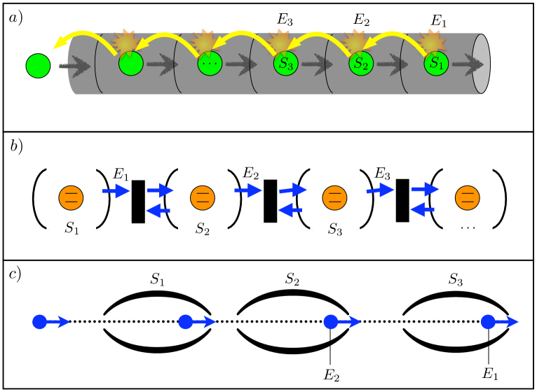
Figure 1: (Color online) Prototypical examples of quantum systems which admit a representation in terms of cascade quantum master equations. a) A string of quantum information carriers (say the photon pulses represented by the green element of the figure) propagating along a fiber while losing photons along the way. Here the sub-environment $E_{1},E_{2},\cdots$ are associated with different sectors of the fiber which effectively describe the transmission line within a lumped model approach. If the propagation speed of the pulses is sufficiently high, the excitations they waste in a given sector of the fiber cannot be re-absorbed by the same pulse: still the subsequent pulses have a certain probability of absorbing it. The net result is an indirect, unidirectional coupling between the pulses mediated by the fiber which allow quantum signals to pass from one carrier to the subsequent ones as schematically shown by the yellow arrows of the figure. b) A set of atoms or ions (represented by the orange elements in the figure) trapped into a series of QED cavities which exchange photons (blue arrows), via unidirectional couplers (black elements) [10, 11]. c) An array of cavities $S_{1},S_{2},\cdots$ crossed sequentially by atoms $E_{1},E_{2},\cdots$ (blue elements) of a beam. The injection rate is such that the atoms cross the cavities one by one. The atoms are initially prepared all in the same state.

The manuscript is organized as follows. In Sec. 2 we describe the collisional model, its continuous time limit (Sec. 2.1) and the basics properties of the associated master equation for cascade quantum systems. In Sec. 3 we then pass to discuss the fundamental assumption which underline the derivation (namely the environment stability condition under collisions). Here we first show how local free evolution term can be embedded in the derivation (Sec. 3.1). Then we prove that the stability condition can always be enforced by passing through an interaction picture representation which defines a more “stable” effective coupling with the environment (Sec. 3.2). Conclusions and final remarks are presented in Sec. 4.

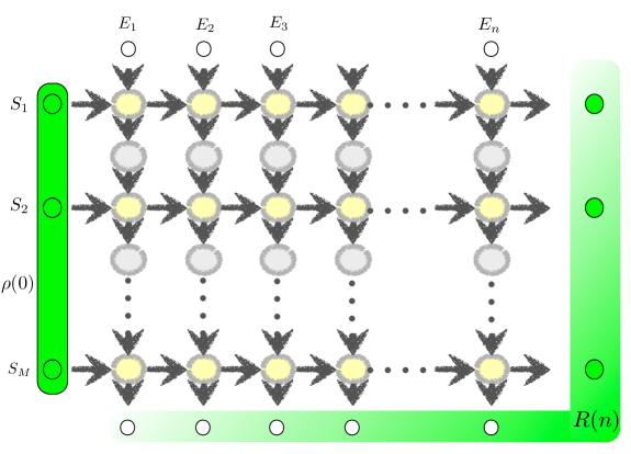
Figure 2: (Color online) Schematic of the collisional model. The horizontal lines describe an ordered set of carriers $S_{1},S_{2},\cdots$ which interact with an ordered set of (possibly infinite) identical local sub-environments $E_{1},E_{2},\cdots$ via local unitaries $\mathcal{U}_{S_{m}E_{n}}$ represented by the yellow elements ($\eta$ being the initial state of the $E_{j}$s). Between collisions each sub-environment evolves according to the “damper” maps $\mathcal{M}$ (represented in the figure by the grey elements). The overall dynamics can be described as a ordered sequence of row or of column super-operators – see Fig. 3 for details.

2 The collisional model

Consider a multipartite quantum system ${\cal S}$, composed by $M$ - not necessarily identical - ordered subsystem $S_{1},S_{2}\cdots S_{M}$ which we shall refer to as the information carriers of the model. They are assumed to be prepared in a possibly entangled initial state $\rho(0)$ and to evolve in time due to the interactions with a multipartite environment ${\cal E}$ consisting of a collection of sub-environments $E_{1},E_{2},\cdots$. Following the collision model of irreversible dynamics presented in Refs. [18, 19], the carriers/sub-enviroment couplings are described via a sequence of pairwise, time-ordered unitary interactions which in our case are organized as in the scheme shown in Fig. 2. According to it, each element of ${\cal S}$ interacts with all the elements of ${\cal E}$ in such a way that given $m^{\prime}\geqslant m$ and $n^{\prime}\geqslant n$ integers, the “collision” between $S_{m}$ and $E_{n}$ is assumed to happen before the one involving $S_{m^{\prime}}$ and $E_{n^{\prime}}$. In particular, this implies that the $S_{1},E_{1}$ interaction takes place before the couplings between $S_{1},E_{2}$, the coupling between $S_{2},E_{1}$, and the coupling between $S_{2},E_{2}$. Similarly the $S_{2},E_{2}$ coupling is assumed to come after the $S_{2},E_{1}$ and the $S_{1},E_{2}$ couplings, while no specific ordering is imposed on these last two events. Within this theoretical framework the temporal evolution of $m$-th carrier $S_{m}$ can be then be described trough the action of the following joint unitary evolution

$$U_{S_{m}{\cal E}}^{(n)}:=U_{S_{m},E_{n}}\;U_{S_{m},E_{n-1}}\;\cdots\;U_{S_{m},E_{2}}\;U_{S_{m},E_{1}}\;,$$ (1)

where, for instance,

$$U_{S_{m},E_{n}}:=\exp[-igH_{S_{m}E_{n}}\Delta t]\;,$$ (2)

is the transformation that characterizes the “collision” between $S_{m}$ and $E_{m}$. In this expression $\Delta t$ is the collision time, $g$ is an intensity parameter that gauges the strength of the coupling, while $H_{S_{m}E_{n}}$ is the coupling Hamiltonian which, without loss of generality, we write as

$$H_{S_{m}E_{n}}:=\sum_{\ell}\;A^{(\ell)}_{S_{m}}\otimes B^{(\ell)}_{E_{n}}\;,$$ (3)

with $A^{(\ell)}_{S},B^{(\ell)}_{E}$ being Hermitian operators. It is worth stressing that in writing Eq. (1) one implicitly assumes that a given carrier never interact twice with the same sub-enviroment. This hypothesis is typically enforced in collisional models which aim to describe Markovian processes – see however Ref. [20] for an alternative approach. Its validity relies on the existence of a two well separated time scales: a fast one, which defines the typical correlation times of the environment, and a slow one, which instead defines the dissipative effects on the system of interest (i.e. the carriers) induced by the coupling with the bath. Such assumption of course is not always fulfilled and when enforced it inhibits the possibility of feedback mechanisms where the state of the system at a given time is influenced by the entire evolution history. Notice however that in the scenario we are considering here, the global Markovian structure of the coupling (1) doesn’t prevent the possibility that different carriers could have a non trivial causal influence on each other. In other words, as schematically shown in Fig. 1 a), quantum “information” can be transferred from one carrier to the other through the intermediation of the environment.

In top of the processes described by the unitary couplings (1) we also assume that between two consecutive collisions each sub-environment evolves according to the action of a local Completely Positive (CP) map $\mathcal{M}$. The latter is introduced to effectively account for the internal dynamics of ${\cal E}$: in particular the transformations $\mathcal{M}$ mimics the relaxation processes that may take place within the environment alone (e.g. originating from the mutual interactions between its various parts) and which in principle involve timescales different from those that define the rate of the collisional events. In other words, as in Ref. [5], the mappings ${\cal M}$ act as “dampers” for the information that percolates from one carrier to the subsequent one: how effective such damping is, it depends of course upon the rate at which two subsequent carriers approach the same sub-environemnt (i.e. in the example of Fig. 1 a), it depends upon the propagation velocity of the pulses along the fiber). Putting all together the resulting temporal evolution can hence be expressed in a compact form by observing that after the interactions with the first $n$ elements of ${\cal E}$ the global state $R(n)$ of the system and of the environment is obtained from the initial state $\rho(0)\otimes\eta^{\otimes n}$ as

$$R(n)={\cal W}^{(n,M)}(\rho(0)\otimes\eta^{\otimes n})\;,$$ (4)

where ${\cal W}^{(n,M)}$ is the super-operator which describes the collisions and the free evolutions of ${\cal E}$ while $\eta$ is the density matrix which describes the initial state of the sub-environments (for simplicity we assumed that all the $E_{n}$ are characterized by the same initial state).

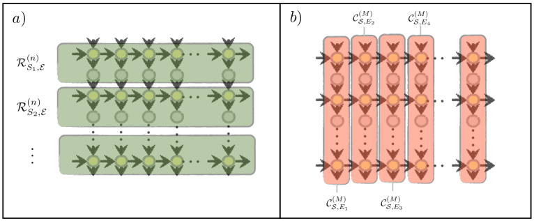
Figure 3: (Color online) Schematic of the decomposition of the evolution map ${\cal W}^{(n,M)}$ collisional model in terms of a) row operators as detailed in Eq. (5) (in the figure these operators are represented by the gray elements), or b) column operators (represented by the red elements) as detailed in Eq. (7).

The ${\cal W}^{(n,M)}$ can be expressed as a composition of row super-operators stack in series one on top of the other (see Fig. 3)

$${\cal W}^{(n,M)}={\cal R}^{(n)}_{S_{M},{\cal E}}\circ{\cal R}^{(n)}_{S_{M-1},{\cal E}}\circ\cdots\circ{\cal R}^{(n)}_{S_{2},{\cal E}}\circ{\cal R}^{(n)}_{S_{1},{\cal E}}\;,$$ (5)

where we use the symbol “$\circ$” to represent the composition of super-operators and where

$${\cal R}^{(n)}_{S_{m},{\cal E}}:={\cal M}^{\otimes n}\;\circ\;{\cal U}_{S_{m},{\cal E}}^{(n)}\;.$$ (6)

In the above expression, given a unitary transformation $U$, we define ${\cal U}(\cdots)=U(\cdots)U^{\dagger}$, while we used the symbol ${\cal M}^{\otimes n}$ to represent ${\cal M}_{E_{1}}\circ\cdots\circ{\cal M}_{E_{n}}$, ${\cal M}_{E_{j}}$ being the map ${\cal M}$ operating on the $j$-th element ${E}_{j}$ of ${\cal E}$. The transformation ${\cal R}^{(n)}_{S_{m},{\cal E}}$ describes the evolution of $S_{m}$ in its interaction with ${\cal E}$ plus the subsequent free evolution of the latter induced by the maps $\cal M$. Alternatively, exploiting the fact that for $m^{\prime}\neq m$, $n^{\prime}\neq n$ the operators $U_{S_{m},E_{n}}$ and $U_{S_{m^{\prime}},E_{n^{\prime}}}$ commute, ${\cal W}^{(n,M)}$ can also be expressed in terms of column super-operators concatenated in series as follows:

$${\cal W}^{(n,M)}={\cal C}^{(M)}_{{\cal S},E_{n}}\circ{\cal C}^{(M)}_{{\cal S},E_{n-1}}\circ\cdots\circ{\cal C}^{(M)}_{{\cal S},E_{2}}\circ{\cal C}^{(M)}_{{\cal S},E_{1}}\;,$$ (7)

where for all $j=1,\cdots,n$,

$${\cal C}^{(M)}_{{\cal S},E_{j}} := {\cal M}_{E_{j}}\circ{\cal U}_{S_{M},E_{j}}\circ\cdots\circ{\cal M}_{E_{j}}\circ{\cal U}_{S_{1},E_{j}}\;.$$ (8)

Equations (5) and (8) enlighten the causal structure of the model. In particular (5) makes it explicit that whatever happens to $S_{m+1}$ comes always after the transformations operating on $S_{m}$. As a consequence the latter can have indirect influence on the former but the vice-versa is not allowed. Similarly Eq. (8) shows that an analogous causal structure is present on the elements of ${\cal E}$: events involving $E_{n}$ may have causal influence on those involving $E_{n+1}$ but the opposite is impossible. This last equation is also useful to write a recursive expression for $R(n)$. Indeed by construction we have

$$R(n+1) = {\cal C}^{(M)}_{{\cal S},E_{n+1}}(R(n)\otimes\eta)\;,$$ (9)

which confirms the intrinsic Markovian structure of the temporal evolution for the whole set of carriers that composes ${\cal S}$. The recursive form of Eq. (9) is similar to the one characterizing the models of Refs. [19] where, for a single qubit carrier ($M=1$) and for a particular class of interaction unitaries, it was shown that it leads to a dynamics which can be described by a Lindblad super-operator. Following Ref. [17] one can generalize this fact to an arbitrary number of carriers and for arbitrary coupling Hamiltonians (3). We simply assume a weak coupling regime where we take a proper expansion with respect to the parameters $g$ and $\Delta t$ which quantifies the intensity and the duration of the single events. In particular we work in the regime in which $g\Delta t$ is small enough to allow for the expansion of the dynamical equation (9) up to ${\cal O}\big{(}(g\Delta t)^{2}\big{)}$, i.e.

$$R(n+1)=\big{[}{\cal I}_{{\cal S},E_{n+1}} + {\cal C}^{\prime}_{{\cal S},E_{n+1}}g\Delta t$$

$$+ {\cal C}^{\prime\prime}_{{\cal S},E_{n+1}}(g\Delta t)^{2}\big{]}(R(n)\otimes\eta)+{\cal O}\big{(}(g\Delta t)^{3}\big{)}\;,$$

where ${\cal I}_{{\cal S},E_{n+1}}$ is the identity superoperator while ${\cal C}^{\prime}_{{\cal S},E_{n+1}}$ and ${\cal C}^{\prime\prime}_{{\cal S},E_{n+1}}$ are the first and second expansion terms in $g\Delta t$ of the superoperator ${\cal C}^{(M)}_{{\cal S},E_{n+1}}$, respectively (see below). The resulting expression can then be traced over the degree of freedom of ${\cal E}$ to get an equivalent expression for the the reduced density matrix of ${\cal S}$ alone, yielding,

$$\rho(n+1) = \rho(n)+(g\Delta t)\left\langle{\cal C}^{\prime}_{{\cal S},E_{n+1}}\big{(}R(n)\otimes\eta\big{)}\right\rangle_{\cal E}$$

$$\qquad+(g\Delta t)^{2}\left\langle{\cal C}^{\prime\prime}_{{\cal S},E_{n+1}}\big{(}R(n)\otimes\eta\big{)}\right\rangle_{\cal E}+{\cal O}\big{(}(g\Delta t)^{3}\big{)}\;,$$

where we used the symbol $\langle\cdots\rangle_{\cal E}$ to represent the partial trace over $E_{1},E_{2},\cdots$ and where for all $n$ we introduced

$$\rho(n):=\langle R(n)\rangle_{\cal E}\;,$$ (12)

(it represents the joint state of the carriers after the interaction with the first $n$ sub-environment). Explicit expressions can be obtained by noticing that for each $m$ and $j$, the super-operators ${\cal U}_{S_{m},E_{j}}$ admit the following expansion,

$${\cal U}_{S_{m},E_{j}}={\cal I}_{S_{m},E_{j}}+(g\Delta t)\;{\cal U}_{S_{m},E_{j}}^{\prime}+(g\Delta t)^{2}\;{\cal U}_{S_{m},E_{j}}^{\prime\prime}+{\cal O}\big{(}(g\Delta t)^{3}\big{)}\;,$$ (13)

with

$${\cal U}_{S_{m},E_{j}}^{\prime}(\cdots):=-i\Big{[}H_{S_{m},E_{j}},(\cdots)\Big{]}_{-}\;,$$ (14)

$${\cal U}_{S_{m},E_{j}}^{\prime\prime}(\cdots):=H_{S_{m},E_{j}}(\cdots)H_{S_{m},E_{j}}-\frac{1}{2}\Big{[}H_{S_{m},E_{j}}^{2},(\cdots)\Big{]}_{+}\;,$$ (15)

where $[\cdots,\cdots]_{-}$ and $[\cdots,\cdots]_{+}$ represent the commutator and the anti-commutator brackets respectively. From Eq. (8) it then follows that

$${\cal C}_{{\cal S},E_{j}}^{\prime} := \sum_{m=1}^{M}{\cal M}_{E_{j}}^{M-m+1}\circ{\cal U}_{S_{m},E_{j}}^{\prime}\circ{\cal M}_{E_{j}}^{m-1}\;,$$ (16)

$${\cal C}_{{\cal S},E_{j}}^{\prime\prime} := {\cal C}_{{\cal S},E_{j}}^{\prime\prime,a}+{\cal C}_{{\cal S},E_{j}}^{\prime\prime,b}\;,$$ (17)

with

$${\cal C}_{{\cal S},E_{j}}^{\prime\prime,a} := \sum_{m=1}^{M}{\cal M}_{E_{j}}^{M-m+1}\circ{\cal U}_{S_{m},E_{j}}^{\prime\prime}\circ{\cal M}_{E_{j}}^{m-1}\;,$$

$${\cal C}_{{\cal S},E_{j}}^{\prime\prime,b} := \sum_{m^{\prime}=m+1}^{M}\sum_{m=1}^{M-1}{\cal M}_{E_{j}}^{M-m^{\prime}+1}\circ{\cal U}_{S_{m^{\prime}},E_{j}}^{\prime}\circ{\cal M}_{E_{j}}^{m^{\prime}-m}\circ{\cal U}_{S_{m},E_{j}}^{\prime}\circ{\cal M}_{E_{j}}^{m-1}\;,$$ (18)

(here ${\cal M}_{E}^{m}$ stands for the iterated application of $m$ maps ${\cal M}$ on the same sub-environmental system $E$, e.g. ${\cal M}_{E}^{2}={\cal M}_{E}\circ{\cal M}_{E}$). Replacing these expressions into Eq. (2) and remembering the definition (3) the first order term in $g\Delta t$ gives

$$\left\langle{\cal C}^{\prime}_{{\cal S},E_{n+1}}\big{(}R(n)\otimes\eta\big{)}\right\rangle_{\cal E}=-i\Big{[}\sum_{m}H_{m}^{(eff)},\rho(n)\Big{]}_{-}\;,$$ (19)

with $H_{m}^{(eff)}$ being the following effective local Hamiltonians

$$H_{m}^{(eff)}:=\sum_{\ell}\;\left\langle B^{(\ell)}_{E_{n+1}}{\cal M}_{E_{n+1}}^{m-1}(\eta)\right\rangle_{E_{n+1}}\;A^{(\ell)}_{S_{m}}\;.$$ (20)

For the second order terms in $g\Delta t$ we get instead two contributions associated respectively to local Lindblad terms (i.e. Lindblad terms which act locally on the $m$-th carrier) and two-body non local terms which couple the $m$ carrier to the $m^{\prime}>m$. More precisely the first one is given by

$$\left\langle{\cal C}^{\prime\prime,a}_{{\cal S},E_{n+1}}\big{(}R(n)\otimes\eta\big{)}\right\rangle_{\cal E}=\frac{1}{\gamma}\;\sum_{m}{\cal L}_{m}(\rho(n))\;,$$ (21)

where $\gamma$ is a positive parameter whose value will be specified later (see Eq. (29) below), while ${\cal L}_{m}$ is the super-operator

$${\cal L}_{m}(\cdots) = \frac{1}{2}\sum_{\ell,\ell^{\prime}}{\gamma_{m}^{(\ell,\ell^{\prime})}}\big{[}2A_{S_{m}}^{(\ell^{\prime})}(\cdots)A_{S_{m}}^{(\ell)}$$ (22)

$$-A^{(\ell)}_{S_{m}}A^{(\ell^{\prime})}_{S_{m}}(\cdots)-(\cdots)A^{(\ell)}_{S_{m}}A^{(\ell^{\prime})}_{S_{m}}\big{]}\;.$$

In this expression the coefficients

$$\gamma^{(\ell,\ell^{\prime})}_{m}:=\gamma\;\langle B_{E}^{(\ell)}B_{E}^{(\ell^{\prime})}\;{\cal M}_{E}^{m-1}(\eta)\rangle_{E}\;,$$ (23)

define the (non negative) correlation matrix of the sub-environment operators $B_{E}^{(\ell)}$ and $B_{E}^{(\ell^{\prime})}$ evaluated on the density matrix ${\cal M}^{m-1}(\eta)$ which describes the state of the sub-environment after $m-1$ free (i.e. non collisional) evolution steps. Equation (22) can also be casted in a more traditional form [21] by diagonalizing $\gamma^{(\ell,\ell^{\prime})}_{m}$: this allows one to identify the decay rates of the system with the non-negative eigenvalues $r^{(\ell)}_{m}$ of $\gamma^{(\ell,\ell^{\prime})}_{m}$ and the associated Lindblad operators $L_{S_{m}}^{(\ell)}$ with a proper linear combinations of the $A_{S_{m}}^{(\ell)}$.

The second contribution of order two in $g\Delta t$ which enters Eq. (2) is instead given by

$$\left\langle{\cal C}^{\prime\prime,b}_{{\cal S},E_{n+1}}\big{(}R(n)\otimes\eta\big{)}\right\rangle_{\cal E}=\frac{1}{\gamma}\;\sum_{m^{\prime}>m}\;{\cal D}^{(\rightarrow)}_{m,m^{\prime}}(\rho(n))\;,$$ (24)

where for $m^{\prime}>m$ ${\cal D}^{(\rightarrow)}_{m,m^{\prime}}$ is the super-operator defined as

$${\cal D}^{(\rightarrow)}_{m,m^{\prime}}(\cdots) = \sum_{\ell,\ell^{\prime}}\gamma_{m,m^{\prime}}^{(\ell,\ell^{\prime})}\;\;A_{S_{m}}^{(\ell)}\;\Big{[}(\cdots),A_{S_{m^{\prime}}}^{(\ell^{\prime})}\Big{]}_{-}$$ (25)

$$-\sum_{\ell,\ell^{\prime}}[\gamma_{m,m^{\prime}}^{(\ell,\ell^{\prime})}]^{*}\;\;\Big{[}(\cdots),A_{S_{m^{\prime}}}^{(\ell^{\prime})}\Big{]}_{-}\;A_{S_{m}}^{(\ell)}\;,$$

with

$$\gamma^{(\ell,\ell^{\prime})}_{m,m^{\prime}}:=\gamma\;\langle B_{E}^{(\ell^{\prime})}{\cal M}^{m^{\prime}-m}(B_{E}^{(\ell)}\;{\cal M}^{m-1}(\eta))\;\rangle_{E}\;.$$ (26)

The coefficients $\gamma^{(\ell,\ell^{\prime})}_{m,m^{\prime}}$ introduce cross correlations among the carriers and depend upon the distance $m^{\prime}-m$ between the associated rows of the graph of Fig. 2. Furthermore, similarly to the the terms of Eq. (23), they also depend on $m-1$ due to the fact that the model admits a first carrier.

The resulting expression for $\rho(n+1)$ can thus be written as

$$\frac{\rho(n+1)-\rho(n)}{\Delta t}=-ig\Big{[}\sum_{m}H_{m}^{(eff)},\rho(n)\Big{]}_{-}$$

$$\qquad+\frac{g^{2}\Delta t}{\gamma}\;\left\{\sum_{m}{\cal L}_{m}(\rho(n))+\sum_{m^{\prime}>m}{\cal D}^{(\rightarrow)}_{m,m^{\prime}}(\rho(n))\right\}\;+{\cal O}\big{(}g^{3}\Delta t^{2}\big{)}\;,$$ (27)

which possesses an explicit Markovian structure characterized by the presence of an effective Hamiltonian (first line) and dissipative contributions (second line).

Before proceeding to the continuos limit let us briefly review how the above scheme applies to a specific discrete system, with the aim to clarify the meaning and the validity of the assumptions made in our model. For this purpose we refer to the prototypical example of Fig. 1 c). Here an array of cavities is driven by a beam of atoms crossing them. The rate of injection of the atoms is such that the atoms enter the cavity one by one as shown in figure. The atoms in the beam, all initially prepared in the same state cross sequentially all the cavities of the array. The atom-field interaction is described by the Jaynes-Cummings hamiltonian, which can be straightforwardly cast in the form (3). For a single cavity crossed by a beam of single atoms, in the absence of leackage of photons out of the cavity, such model describes damping or amplification for the cavity field, whose dynamics can be described by a Markovian master equation in Lindblad form [22]. The extension to $n$ cavity is described naturally in our model. Such markovian behavior is due to two crucial features of the model: the short (finite) time $\Delta t$ which takes each atom to cross a cavity and the fact that the atomic state is “refreshed” when a new atom is injected. The master equation so obtained describes a coarse grained time derivative on a timescale $\Delta t$. On such time scale the environment is reset. In the standard theory of damping of a system which is continuosly interacting with the same - big - reservoir the time $\Delta t$ would be the self correlation time of the reservoir. This is not the case in our scenario: each sub environment is small but it interacts for a short time and then, after a time $\Delta t$ substituted with a new one. Furthermore the cross terms in our master equation do not describe a collective, simultaneous, coupling of the subsystems with the environment, but rather they describe how the dynamics of the various subsystems are correlated due to the fact that they have interacted sequentially with the sub environments. This explains why the dynamics described by our system is markovian and does not exhibit the non markovian multipartite features which are characteristic of the scenarios analyzed in [23].

2.1 Continuous limit

Equation (27) can be turned into a continuos time expression by taking the proper limit $\Delta t\rightarrow 0$ while sending $n$ to infinity so that

$$\lim_{\Delta t\rightarrow 0^{+}}n\;\Delta t=t\;.$$ (28)

Notice that there are two possible regimes. If $g$ is kept constant as $\Delta t$ goes to zero, then the dissipative contributions of Eq. (27) are washed away and the dynamics reduces to a unitary evolution characterized by the effective (possibly time-dependent) Hamiltonian (20). The situation becomes more interesting if instead $g$ is sent to infinity so that $g^{2}\Delta t$ remains finite, i.e. [17]

$$\lim_{\Delta t\rightarrow 0^{+}}g^{2}\Delta t=\gamma\;.$$ (29)

Enforcing this limit is of course problematic due to the presence of the first order contribution in Eq. (27) which tends to explode. A way out is to assume the following stability condition for the environment [17],

$$~{}\langle B_{E}^{(\ell)}{\cal M}^{m}(\eta)\rangle_{E}=0\qquad\forall\ell,m\;,$$ (30)

which ensures that $H_{m}^{(eff)}$, and hence the first order contribution of Eq. (27), identically nullifies. Under this hypothesis, defining $\rho(t)=\lim_{\Delta t\rightarrow 0^{+}}\;\rho(n)$, one can indeed arrive to the following continuous master equation for the system,

$${\dot{\rho}}(t)=\sum_{m=1}{\cal L}_{m}(\rho(t))+\sum_{m^{\prime}>m}{\cal D}^{(\rightarrow)}_{m,m^{\prime}}(\rho(t))\;,$$ (31)

whose properties have been characterized in Ref. [17]. Here we only mention that the cross terms appearing in Eq. (31) have an intrinsic unidirectional character which makes this expression suitable to characterize the dynamics of a cascade quantum system. Indeed, for each $m^{\prime}>m$ it can be directly verified from Eq. (25) that we have

$$\left\langle{\cal D}^{(\rightarrow)}_{m,m^{\prime}}(\cdots)\right\rangle_{S_{m^{\prime}}}=0\;.$$ (32)

This implies that the evolution of the first $m$ carriers of the system are not influenced by the evolution of the ones that follow (in other words it is possible to write a master equation for the density matrix of the first $m$ elements of ${\cal S}$ only). The opposite relation however is not true as in general ${\cal D}^{(\rightarrow)}_{m,m^{\prime}}$ doesn’t nullify when traced over $S_{m}$, i.e. $\left\langle{\cal D}^{(\rightarrow)}_{m,m^{\prime}}(\cdots)\right\rangle_{S_{m}}\neq 0$. This means in particular that in our model it is in general impossible to write a master equation that involves only the density matrix of the $m^{\prime}$-th carrier $S_{m^{\prime}}$ (we need indeed to include also the carriers that precede it). Similar properties were obtained in the works of Gardiner, Parkins and Carmichael [10] in theirs seminal study of cascade optical quantum systems. As shown in Ref. [17] the latter can be seen as special instances of (31) for specific choices of the couplings (3) and of the environment initial state $\eta$.

In what follows we will not discuss further the implications of Eq. (32). Instead we will focus on the assumption Eq. (30) showing how it can be enforced by passing in a proper interaction picture with respect to the free evolution of the carriers. Before doing so however we think it is worth stressing that the above derivation still holds also if the collisional Hamiltonians (3) are not uniform. For instance suppose we have

$$H_{S_{m}E_{n}}:=\sum_{\ell}\;A^{(n,\ell)}_{S_{m}}\otimes B^{(m,\ell)}_{E_{n}}\;,$$ (33)

where now the operators acting on the carrier $S_{m}$ are allowed to explicitly depends upon the $n$ index which label the collisional events, and similarly the operators acting on the sub-enviroment are allowed to explicitly depends upon the index $m$ which labels the carriers. Under these conditions one can verify that Eq. (27) is still valid even though both the super-operators ${\cal L}_{m}$ and ${\cal D}^{(\rightarrow)}_{m,m^{\prime}}$ become explicit functions of the carriers labels and of the index $n$ which plays the role of a temporal parameter for the reduced density matrix $\rho(n)$. Specifically they are now defined respectively as in Eqs. (21) and (24) with the operators $A^{(n+1,\ell)}_{S_{m}}$ instead of $A^{(\ell)}_{S_{m}}$ and with the coefficients $\langle B_{E}^{(\ell)}B_{E}^{(\ell^{\prime})}\;{\cal M}^{m-1}(\eta)\rangle_{E}$ and $\langle B_{E}^{(\ell^{\prime})}{\cal M}^{m^{\prime}-m}(B_{E}^{(\ell)}\;{\cal M}^{m-1}(\eta))\rangle_{E}$ replaced by $\langle B_{E}^{(m,\ell)}B_{E}^{(m,\ell^{\prime})}\;{\cal M}^{m-1}(\eta)\rangle_{E}$ and $\langle B_{E}^{(m^{\prime},\ell^{\prime})}{\cal M}^{m^{\prime}-m}(B_{E}^{(m,\ell)}\;{\cal M}^{m-1}(\eta))\rangle_{E}$ respectively. Similarly the continuous limit can be enforced as before: in this case however, to account for the non uniformity of the couplings, the condition (30) becomes

$$\left\langle B^{(m,\ell)}_{E}{\cal M}_{E}^{m-1}(\eta)\right\rangle_{E}=0,\quad\forall m,\ell\;.$$ (34)

Furthermore, while taking the limit (28) the operators $A^{(n+1,\ell)}_{S_{m}}$ acquire an explicit temporal dependence which transforms them into a one parameter family of operators. As a result we get a time-dependent master equation characterized by a Lindblad generators which explicitly depends on $t$, i.e.

$${\dot{\rho}}(t)=\sum_{m=1}{\cal L}_{m}(\rho(t);t)+\sum_{m^{\prime}>m}{\cal D}^{(\rightarrow)}_{m,m^{\prime}}(\rho(t);t)\;,$$ (35)

with ${\cal L}_{m}(\cdots;t)$ and ${\cal D}^{(\rightarrow)}_{m,m^{\prime}}(\cdots;t)$ as in Eqs. (22) and (25) with the operators $A^{(\ell)}_{S_{m}}$ replaced by $A^{(\ell)}_{S_{m}}(t):=\lim_{\Delta t\rightarrow 0^{+}}A^{(n+1,\ell)}_{S_{m}}$.

3 The stability condition

The name stability condition given to the constraint (30) follows from the fact that it implicitly assumes that during the collisions the sub-environments are not affected by the coupling with the carriers (at least at first order in the coupling strength). This is mathematically equivalent to the standard derivation of a Markovian master equation [21] for a system interacting with a large environment, in which one assumes that the overall system-environment density operator at any given time $t$ of the evolution factorizes as in $\rho(t)\otimes\eta$ where $\eta$ is the environment density operator. The two scenarios are however different. In the standard case the reason for which the environment state is unchanged is because it is big. In the scenario analyzed here, consistently with the collisional model, the environment state is constant because each subsystem collides briefly with a sequence of sub-environments all initially in the same state.

As anticipated in the previous section, in our analysis of the condition (30) a proper handling of the carriers free evolution plays a fundamental role. This should not come as a surprise: an important step in the standard derivation of a Lindblad form is the possibility of effectively “removing” the free evolution of the system and of the environment by passing in the associated interaction representations. Such step is useful because it allows one to directly relate the fast evolution times of the large environment with the slow decaying rates of the system of interests: it is in this limit that the Markov approximation can be properly enforced . In our model we can show that the cases in which Eq. (30) cannot be directly enforced, can be mapped into effective models in which Eq. (30) exactly holds but which allows for explicit free evolution terms for the carriers between any two collisions which have to be removed by passing in a proper interaction picture representation. As a preliminary step toward the discussion of the stability condition it is hence important to discuss how the derivation changes in this last circumstance.

3.1 Including local free evolution terms for the carriers

Assume that the stability condition (30) holds, but that between any two consecutive collisions, the carriers undergo to a free-evolution described by a (possibly time-depedent) Hamiltonian $H_{{\cal S}}(t):=\sum_{m}h_{S_{m}}(t)$ which are local (i.e. no direct interactions between the carriers is allowed). Under this circumstance it is possible to show that Eq. (31) still holds in the proper interaction picture representation at the price of allowing the generators of the resulting master equation to be explicitly time dependent as in Eq. (35).

To see this we first notice that under the assumption that the collision time $\Delta t$ is much shorter than the time interval that elapses between two consecutive collisional events (i.e. $\Delta t\ll\tau_{n}-\tau_{n-1}$), the unitary operator which describes the evolution of the $m$-th carrier in its interaction with ${\cal E}$ is now given by

$$U_{S_{m}{\cal E}}^{(n)}:=U_{S_{m},E_{n}}V_{S_{m}}(\tau_{n},\tau_{n-1})\;U_{S_{m},E_{n-1}}$$ (36)

$$\qquad\qquad\;\cdots\;V_{S_{m}}(\tau_{2},\tau_{1})\;U_{S_{m},E_{2}}\;V_{S_{m}}(\tau_{1},0)\;U_{S_{m},E_{1}},$$

where $U_{S_{m},E_{n}}$ are the collisional transformations, $\tau_{n}$ is the time at which the $n$-th collision takes place, and where $V_{S_{m}}(\tau_{n},\tau_{n-1}):={\cal T}\exp[-i\int_{\tau_{n-1}}^{\tau_{n}}dt^{\prime}h_{S_{m}}(t^{\prime})]$ is the unitary operator which describes the free-evolution of $S_{m}$ between the $(n-1)$-th and the $n$-th collision (in this expression ${\cal T}\exp[\cdots]$ indicates the time-ordered exponential which we insert to explicitly account for possibility that the $h_{S_{m}}$ will be time-dependent). Define hence the operators

$$\bar{A}^{(n,\ell)}_{S_{m}}:=V_{S_{m}}^{\dagger}(\tau_{n},0)\;{A}^{(\ell)}_{S_{m}}\;V_{S_{n}}(\tau_{n},0)\;,$$ (37)

and the Hamiltonian

$$\bar{H}_{S_{m},E_{n}}:=V_{S_{n}}^{\dagger}(\tau_{n},0)\;{H}_{S_{m},E_{n}}V_{S_{n}}(\tau_{n},0)=\sum_{\ell}\;\bar{A}^{(n,\ell)}_{S_{m}}\otimes B^{(\ell)}_{E_{n}}\;,$$ (38)

which describes the coupling between $S_{m}$ and ${\cal E}$ in the interaction representation associated with the free evolution of $S_{m}$. Notice that the operators $\bar{A}^{(n,\ell)}_{S_{m}}$ are explicit functions of the index $n$ which labels the collisions as in the case of Eq. (33) (here however the terms operating on ${\cal E}$ are kept uniform). Observing that for all $\ell$ one has $V_{S_{m}}(\tau_{\ell},\tau_{\ell-1})V_{S_{m}}(\tau_{\ell-1},\tau_{\ell-2})=V_{S_{m}}(\tau_{\ell},\tau_{\ell-2})$ we can now write Eq. (36) as

$$U_{S_{m}{\cal E}}^{(n)}:=V_{S_{m}}(\tau_{n},0)\;\bar{U}_{S_{m},{\cal E}}^{(n)},$$ (39)

where $\bar{U}_{S_{m},{\cal E}}^{(n)}$ is the unitary that defines the collisions of $S_{m}$ with the sub-environments in the interaction representation, i.e.

$$\bar{U}_{S_{m},{\cal E}}^{(n)}:=\bar{U}_{S_{m},E_{n}}\;\bar{U}_{S_{m},E_{n-1}}\cdots\bar{U}_{S_{m},E_{1}},$$ (40)

with

$$\bar{U}_{S_{m},E_{n}}=\exp[-ig\;\bar{H}_{S_{m},E_{n}}\Delta t]\;.$$ (41)

Similarly we can express the super-operators ${\cal W}^{(n,M)}$ as

$${\cal W}^{(n,M)} = {\cal V}_{{\cal S}}(\tau_{n},0)\circ\;\bar{\cal W}^{(n,M)}\;,$$ (42)

$$\bar{\cal W}^{(n,M)} := \bar{\cal C}^{(M)}_{{\cal S},E_{n}}\circ\cdots\circ\bar{\cal C}^{(M)}_{{\cal S},E_{1}}\;,$$ (43)

$$\bar{\cal C}^{(M)}_{{\cal S},E_{j}} := {\cal M}_{E_{j}}\circ\bar{\cal U}_{S_{M},E_{j}}\circ\cdots\circ{\cal M}_{E_{j}}\circ\bar{\cal U}_{S_{1},E_{j}},$$ (44)

with ${\cal V}_{{\cal S}}(\tau_{n},0)$ being the super-operator associated with the joint free unitary evolution obtained by combining all the local terms of the carriers, i.e. $V_{\cal S}(\tau_{n},0):=V_{S_{1}}(\tau_{n},0)\cdots V_{S_{M}}(\tau_{n},0)$. Defining hence $\bar{R}(n)$ the state of ${\cal S}$ and of the first elements of ${\cal E}$ after $n$ collisions in the interaction representation induced by $V_{\cal S}(\tau_{n},0)$ as

$$\bar{R}(n)=V_{\cal S}^{\dagger}(\tau_{n},0)\;R(n)\;V_{\cal S}(\tau_{n},0)\;,$$ (45)

we get a recursive expression analogous to Eq. (9) with ${\cal C}^{(M)}_{{\cal S},E_{n+1}}$ replaced by $\bar{\cal C}^{(M)}_{{\cal S},E_{n+1}}$, i.e.

$$\bar{R}(n+1) = \bar{\cal C}^{(M)}_{{\cal S},E_{n+1}}(\bar{R}(n)\otimes\eta)\;.$$ (46)

More precisely this expression coincides with that which, as in the case described at the end of Sec. 2.1, one would have obtained starting from a collisional model in which no free evolution of the carriers is allowed but the collisional events are not uniform. Indeed the generators of the dynamics $\bar{H}_{S_{m},E_{n}}$ do have the same form of the Hamiltonians (33). Following the same prescription given there, we can then get an expression for the reduced density matrix $\bar{\rho}(n)=\langle\bar{R}(n)\rangle_{\cal E}$ which represents the state of the carriers after $n$ collisions in the interaction picture with respect to the free evolution generated by $H_{\cal S}(t)$. Enforcing the limit (29) under the condition (34), one can verify that $\bar{\rho}(t)$ obeys to a ME analogous to Eq. (31) with the operators $A_{S_{m}}^{(\ell^{\prime})}$ being replaced by the time-dependent operators $\bar{A}^{(\ell)}_{S_{m}}(t):=\lim_{\Delta t\rightarrow 0^{+}}\bar{A}^{(n,\ell)}_{S_{m}}$.

3.2 Enforcing the stability condition via a global unitary mapping

Now that we have learned how to deal with free local evolutions terms operating between the collisional events, we show how to use this result to effectively enforce the stability condition of Eq. (30) for models in which it doesn’t apply rigorously. Specifically we shall see that such condition can be imposed by first moving into an interaction representation with respect to a rescaled local Hamiltonian for the system ${\cal S}$ which maps the problem into one equivalent to that discussed in Sec. 3.1.

Indeed let

$$H_{S_{m}E_{n}}:=\sum_{\ell}\;A^{(n,\ell)}_{S_{m}}\otimes B^{(\ell)}_{E_{n}}\;,$$ (47)

be the Hamiltonian which describe the collisions between the carriers and the sub-environments (notice that we are allowing the operators $A^{(n,\ell)}_{S_{m}}$ to depend explicitly from the $n$ label to account for possible local free evolution of the carriers as discussed in the previous section). Suppose then that Eq. (30) does not hold. In this case we define

$$B^{(m,\ell)}_{E} := B^{(\ell)}_{E}-\delta_{m}^{(\ell)}\;I_{E}\;,$$ (48)

$$\delta_{m}^{(\ell)} := \langle B_{E}^{(\ell)}{\cal M}^{m-1}(\eta)\rangle_{E}\;,$$ (49)

and write,

$$H_{S_{m},E_{n}} := \Delta H_{S_{m},E_{n}}+h_{S_{m}}^{(n)}\;,$$ (50)

where

$$h_{S_{m}}^{(n)}:=\sum_{\ell}\delta_{m}^{(\ell)}\;A^{(n,\ell)}_{S_{m}}\otimes I_{E_{n}}\;,$$ (51)

is a local Hamiltonian on $S_{m}$ while

$$\Delta H_{S_{m},E_{n}}:=\sum_{\ell}\;A^{(n,\ell)}_{S_{m}}\otimes B^{(m,\ell)}_{E_{n}}\;,$$ (52)

is a rescaled coupling Hamiltonian. Differently from the original one given in Eq. (47), but similarly to Eq. (33), it is built from operators $B^{(m,\ell)}_{E_{n}}$ which explicitly depend on the label $m$ of the carrier $S_{m}$, and which by construction satisfy the generalized condition (34), i.e.

$$\langle B_{E}^{(m,\ell)}\;{\cal M}^{m-1}(\eta)\rangle_{E}=0\;.$$ (53)

Passing then in the interaction representation with respect to $h_{S_{m}}^{(n)}$ we can thus express the unitary evolution induced by $H_{S_{m},E_{n}}$ as

$$U_{S_{m},E_{n}}=\exp[-igH_{S_{m},E_{n}}\Delta t]=e^{-igh_{S_{m}}^{(n)}\Delta t}\;{\cal T}\exp[-ig\int_{0}^{\Delta t}dt^{\prime}\;\overline{\Delta H}_{S_{m},E_{n}}(t^{\prime})]\;,$$

where $e^{-igh_{S_{m}}^{(n)}\Delta t}$ is a local unitary on $S_{m}$ while

$$\overline{\Delta H}_{S_{m},E_{n}}(t) := e^{igh_{S_{m}}^{(n)}t}\;{\Delta H}_{S_{m},E_{n}}\;e^{-igh_{S_{m}}^{(n)}t}\;.$$

Therefore the rhs of Eq. (1) can be written now as

$$U_{S_{m},{\cal E}}^{(n)}=V_{S_{m}}^{(n)}\;\tilde{U}_{S_{m},E_{n}}\;\cdots\;\tilde{U}_{S_{m},E_{2}}\;\tilde{U}_{S_{m},E_{1}}\;,$$ (54)

where $V_{S_{m}}^{(n)}$ and $\tilde{U}_{S_{m},E_{j}}$ are the following unitary operators

$$V_{S_{m}}^{(n)}:=e^{-igh_{S_{m}}^{(n)}\Delta t}\;e^{-igh_{S_{m}}^{(n-1)}\Delta t}\cdots e^{-igh_{S_{m}}^{(2)}\Delta t}\;e^{-igh_{S_{m}}^{(1)}\Delta t}\;,$$ (55)

and

$$\tilde{U}_{S_{m},E_{j}}:=[V_{S_{m}}^{(j-1)}]^{\dagger}\;\left({\cal T}\exp[-ig\int_{0}^{\Delta t}dt^{\prime}\;\overline{\Delta H}_{S_{m},E_{j}}(t^{\prime})]\right)\;V_{S_{m}}^{(j-1)}.$$ (56)

For future reference it is worth anticipating that the term within the round brackets admits the following expansion in $\Delta t$,

$$\qquad\quad I_{S_{m},E_{n}}-i(g\Delta t)\;{\Delta H}_{S_{m},E_{j}}-\frac{1}{2}(g\Delta t)^{2}\left({\Delta H}_{S_{m},E_{j}}\right)^{2}-\frac{i}{2}(g\Delta t)^{2}\;{Q}_{S_{m},E_{j}}+{\cal O}(\Delta t^{3})\;,$$

where the last contribution originates from the time-ordering in the exponential of Eq. (56) and it is defined in terms of the first derivative of ${\overline{\Delta H}}_{S_{m},E_{j}}(t)$, i.e.

$${Q}_{S_{m},E_{j}}:=\frac{\partial\;{\overline{\Delta H}}_{S_{m},E_{j}}(t)}{\partial t}\Big{|}_{t=0}=ig\Big{[}h_{S_{m}}^{(j)},{{\Delta H}}_{S_{m},E_{j}}\Big{]}_{-}.$$ (57)

This yields the following expansion for the super-operator $\tilde{\cal U}_{S_{m},E_{j}}$ associated to the unitary ${\tilde{U}}_{S_{m},E_{j}}$,

$$\tilde{\cal U}_{S_{m},E_{j}}={\cal I}_{S_{m},E_{j}}+(g\Delta t)\;\tilde{\cal U}_{S_{m},E_{j}}^{\prime}+(g\Delta t)^{2}\;\tilde{\cal U}_{S_{m},E_{j}}^{\prime\prime}+{\cal O}\big{(}(g\Delta t)^{3}\big{)}\;,$$ (58)

with ${\cal I}_{S_{m},E_{j}}$ being the identity map and with

$$\;\tilde{\cal U}_{S_{m},E_{j}}^{\prime}(\cdots) := -i\Big{[}\Delta\hat{H}_{S_{m},E_{j}},(\cdots)\Big{]}_{-}\;,$$ (59)

$$\;\tilde{\cal U}_{S_{m},E_{j}}^{\prime\prime}(\cdots) := \Delta\hat{H}_{S_{m},E_{j}}(\cdots)\Delta\hat{H}_{S_{m},E_{j}}-\frac{1}{2}\Big{[}\Delta\hat{H}_{S_{m},E_{j}}^{2},(\cdots)\Big{]}_{+}-\frac{i}{2}\Big{[}\hat{Q}_{S_{m},E_{j}},(\cdots)\Big{]}_{-}\;,$$ (60)

where for easy of notation in this expression given a generic operator $\Theta_{S_{m},E_{j}}$ we used the notation $\hat{\Theta}_{S_{m},E_{j}}$ to represent its evolution via the unitary $V_{S_{m}}^{(j-1)}$, i.e.

$$\hat{\Theta}_{S_{m},E_{j}}:=[V_{S_{m}}^{(j-1)}]^{\dagger}\Theta_{S_{m},E_{j}}V_{S_{m}}^{(j-1)}\;.$$ (61)

The expression Eq. (60) should be compared with Eq. (15): we notice that due to the presence of the time-ordering in Eq. (56) an extra term is present in the decomposition. We shall see however that when tracing out the sub-environments, such term plays no role in the evolution of the carries (see Eq. (75) below).

With the above identities the row super-operator ${\cal R}^{(n)}_{S_{m},{\cal E}}$ entering in Eq. (5) can thus be expressed as

$${\cal R}_{S_{m},{\cal E}}:={\cal M}^{\otimes n}\circ\left({\cal V}_{S_{m}}^{(n)}\circ\;\tilde{\cal U}_{S_{m},E_{n}}\circ\cdots\circ\tilde{\cal U}_{S_{m},E_{1}}\right)={\cal V}_{S_{m}}^{(n)}\circ\tilde{\cal R}_{S_{m},{\cal E}}\;,$$ (62)

where as usual ${\cal V}_{S_{m}}^{(n)}$ and $\tilde{\cal U}_{S_{m},E_{j}}$ represent the super-operators associated with the unitary transformations ${V}_{S_{m}}^{(n)}$ and $\tilde{U}_{S_{m},E_{j}}$ respectively, and where

$$\tilde{\cal R}_{S_{m},{\cal E}} := {\cal M}^{\otimes n}\circ\;\tilde{\cal U}_{S_{m},E_{n}}\circ\cdots\circ\tilde{\cal U}_{S_{m},E_{1}}\;.$$ (63)

Accordingly Eq. (5) becomes

$${\cal W}^{(n,M)}={\cal V}_{\cal S}^{(n)}\circ\tilde{\cal W}^{(n,M)}\;,$$ (64)

with ${\cal V}_{\cal S}^{(n)}$ being the super-operator associated with the joint unitary ${V}_{\cal S}^{(n)}:={V}_{S_{M}}^{(n)}\otimes\cdots\otimes{V}_{S_{1}}^{(n)}$ and with

$$\tilde{\cal W}^{(n,M)}:=\tilde{\cal R}_{S_{M},{\cal E}}\circ\tilde{\cal R}_{S_{M-1},{\cal E}}\circ\cdots\circ\tilde{\cal R}_{S_{2},{\cal E}}\circ\tilde{\cal R}_{S_{1},{\cal E}}\;.$$ (65)

This can also be written in terms of column super-operators as in Eq. (7). In particular we get

$$\tilde{\cal W}^{(n,M)}=\tilde{\cal C}_{{\cal S},E_{n}}\circ\tilde{\cal C}_{{\cal S},E_{n-1}}\circ\cdots\circ\tilde{\cal C}_{{\cal S},E_{2}}\circ\tilde{\cal C}_{{\cal S},E_{1}}\;,$$ (66)

with

$${\cal C}_{{\cal S},E_{j}} := {\cal M}_{E_{j}}\circ\tilde{\cal U}_{S_{M},E_{j}}\circ\cdots\circ{\cal M}_{E_{j}}\circ\tilde{\cal U}_{S_{1},E_{j}}\;.$$ (67)

Defining now

$$\bar{R}(n):={\cal V}_{\cal S}^{(n)}(R(n))=[{V}_{\cal S}^{(n)}]^{\dagger}R(n){V}_{\cal S}^{(n)}\;,$$ (68)

the state of the carriers and of the first $n$ sub-environemental state in the interaction picture representation induced by the unitary ${V}_{\cal S}^{(n)}$, we have

$${\bar{R}}(n+1)=\tilde{\cal W}^{(n+1,M)}(\rho(0)\otimes\eta^{\otimes{n+1}})=\tilde{\cal C}_{{\cal S},E_{n+1}}({\bar{R}}(n)\otimes\eta)\;.$$ (69)

Take then the partial trace over ${\cal E}$ of this expression and use Eq. (58) to expand $\tilde{\cal C}_{{\cal S},E_{n+1}}$. Defining ${\bar{\rho}}(n)=\langle{\bar{R}}(n)\rangle_{\cal E}$ we get

$${\bar{\rho}}(n+1)={\bar{\rho}}(n)+(g\Delta t)\left\langle\tilde{\cal C}^{\prime}_{{\cal S},E_{n+1}}\big{(}{\bar{R}}(n)\otimes\eta\big{)}\right\rangle_{\cal E}$$ (70)

$$\qquad+(g\Delta t)^{2}\left\langle\tilde{\cal C}^{\prime\prime}_{{\cal S},E_{n+1}}\big{(}{\bar{R}}(n)\otimes\eta\big{)}\right\rangle_{\cal E}+{\cal O}\big{(}(g\Delta t)^{3}\big{)}\;,$$

where $\tilde{\cal C}^{\prime}_{{\cal S},E_{n+1}}$ and $\tilde{\cal C}^{\prime\prime}_{{\cal S},E_{n+1}}$ are respectively the first and second order term of the expansion of $\tilde{\cal C}_{{\cal S},E_{n+1}}$, i.e.

$$\tilde{\cal C}_{{\cal S},E_{j}}^{\prime} := \sum_{m=1}^{M}{\cal M}_{E_{j}}^{M-m+1}\circ\tilde{\cal U}_{S_{m},E_{j}}^{\prime}\circ{\cal M}_{E_{j}}^{m-1}\;,$$ (71)

$$\tilde{\cal C}_{{\cal S},E_{j}}^{\prime\prime} := \tilde{\cal C}_{{\cal S},E_{j}}^{\prime\prime,a}+\tilde{\cal C}_{{\cal S},E_{j}}^{\prime\prime,b}\;,$$ (72)

with

$$\tilde{\cal C}_{{\cal S},E_{j}}^{\prime\prime,a} := \sum_{m=1}^{M}{\cal M}_{E_{j}}^{M-m+1}\circ\tilde{\cal U}_{S_{m},E_{j}}^{\prime\prime}\circ{\cal M}_{E_{j}}^{m-1}\;,$$

$$\tilde{\cal C}_{{\cal S},E_{j}}^{\prime\prime,b} := \sum_{m^{\prime}=m+1}^{M}\sum_{m=1}^{M-1}{\cal M}_{E_{j}}^{M-m^{\prime}+1}\circ\tilde{\cal U}_{S_{m^{\prime}},E_{j}}^{\prime}\circ{\cal M}_{E_{j}}^{m^{\prime}-m}\circ\tilde{\cal U}_{S_{m},E_{j}}^{\prime}\circ{\cal M}_{E_{j}}^{m-1}\;.$$ (73)

As in the case of (2) one can verify that the first order contribution nullifies. Indeed we have

$$\!\!\!\!\!\!\!\!\!\!\!\!\!\!\!\!\!\!\!\!\left\langle\tilde{\cal C}^{\prime}_{{\cal S},E_{n+1}}\big{(}{\bar{R}}(n)\otimes\eta\big{)}\right\rangle_{\cal E}:=-i\;\sum_{m}\left\langle\left[{\Delta\hat{H}}_{S_{m},E_{n+1}},{\bar{R}}(n)\otimes{\cal M}_{E_{n+1}}^{m-1}(\eta)]\right]_{-}\right\rangle_{\cal E}$$

$$=-i\sum_{m}\sum_{\ell}\Big{[}\hat{A}^{(n+1,\ell)}_{S_{m}},{\bar{\rho}}(n)\Big{]}_{-}\left\langle B^{(m,\ell)}_{E_{n+1}}{\cal M}_{E_{n+1}}^{m-1}(\eta)\right\rangle_{E_{n+1}}=0\;,$$ (74)

because of Eq. (53). The remaining terms can be computed as in Eq. (21) and (24). Here we only stress on the fact that the component of $\tilde{\cal U}_{S_{m},E_{j}}^{\prime\prime}$ that depends upon the operator $\hat{Q}_{S_{m},E_{j}}$ (i.e. the extra term of Eq. (60)) do not contribute in the final result. Indeed they only enters in the definition of $\tilde{\cal C}_{{\cal S},E_{j}}^{\prime\prime,a}$ and produce the following term

$$\!\!\!\!\!\!\!\!\!\!\!\!-\frac{i}{2}\;\sum_{m}\left\langle\left[\hat{Q}_{S_{m},E_{n+1}},{\bar{R}}(n)\otimes{\cal M}_{E_{n+1}}^{m-1}(\eta)]\right]_{-}\right\rangle_{\cal E}$$ (75)

$$\qquad=\frac{g}{2}\sum_{m}\left\langle\Big{[}\Big{[}\hat{h}_{S_{m}}^{(n+1)},{{\Delta\hat{H}}}_{S_{m},E_{n+1}}\Big{]}_{-},{\bar{R}}(n)\otimes{\cal M}_{E_{n+1}}^{m-1}(\eta)\Big{]}_{-}\right\rangle_{\cal E}$$

$$\qquad=\frac{g}{2}\sum_{m}\sum_{\ell}\left\langle\Big{[}\Big{[}\hat{h}_{S_{m}}^{(n+1)},\hat{A}^{(n+1,\ell)}_{S_{m}}\otimes B^{(m,\ell)}_{E_{n+1}}\Big{]}_{-},{\bar{R}}(n)\otimes{\cal M}_{E_{n+1}}^{m-1}(\eta)\Big{]}_{-}\right\rangle_{\cal E}$$

$$\qquad=\frac{g}{2}\sum_{m}\sum_{\ell}\Big{[}\Big{[}\hat{h}_{S_{m}}^{(n+1)},\hat{A}^{(n+1,\ell)}_{S_{m}}\Big{]}_{-},{\bar{\rho}}(n)\Big{]}_{-}\;\left\langle B^{(m,\ell)}_{E_{n+1}}{\cal M}_{E_{n+1}}^{m-1}(\eta)\right\rangle_{E_{n+1}}=0\;.$$

In summary Eq. (70) yields

$$\!\!\!\!\!\!\!\!\!\!\!\!\!\!\!\!\!\!\!\!\frac{{\bar{\rho}}(n+1)-{\bar{\rho}}(n)}{\Delta t}=\frac{g^{2}\Delta t}{\gamma}\;\left\{\sum_{m}\bar{\cal L}_{m}({\bar{\rho}}(n))+\sum_{m^{\prime}>m}\bar{\cal D}^{(\rightarrow)}_{m,m^{\prime}}({\bar{\rho}}(n))\right\}\;+{\cal O}\big{(}g^{3}\Delta t^{2}\big{)}\;,$$ (76)

where now

$$\!\!\!\!\!\!\!\!\!\!\!\!\!\!\!\!\!\!\!\!\bar{\cal L}_{m}(\cdots)=\frac{1}{2}\sum_{\ell,\ell^{\prime}}{\gamma_{m}^{(\ell,\ell^{\prime})}}\;\Big{[}2\bar{A}_{S_{m}}^{(n+1,\ell^{\prime})}(\cdots)\bar{A}_{S_{m}}^{(n+1,\ell)}$$

$$-\bar{A}^{(n+1,\ell)}_{S_{m}}\bar{A}^{(n+1,\ell^{\prime})}_{S_{m}}(\cdots)-(\cdots)\bar{A}^{(n+1,\ell)}_{S_{m}}\bar{A}^{(n+1,\ell^{\prime})}_{S_{m}}\Big{]}\;,$$

and

$$\!\!\!\!\!\!\!\!\!\!\!\!\!\!\!\!\bar{\cal D}^{(\rightarrow)}_{m,m^{\prime}}(\cdots) = \sum_{\ell,\ell^{\prime}}\;\gamma^{(\ell,\ell^{\prime})}_{m,m^{\prime}}\;\bar{A}_{S_{m}}^{(n+1,\ell)}\;\Big{[}(\cdots),\bar{A}_{S_{m^{\prime}}}^{(n+1,\ell^{\prime})}\Big{]}_{-}$$

$$-\sum_{\ell,\ell^{\prime}}\left[\gamma^{(\ell,\ell^{\prime})}_{m,m^{\prime}}\right]^{*}\;\;\Big{[}(\cdots),\bar{A}_{S_{m^{\prime}}}^{(n+1,\ell^{\prime})}\Big{]}_{-}\;\bar{A}_{S_{m}}^{(n+1,\ell)}\;,$$

In these expressions the coefficients ${\gamma_{m}^{(\ell,\ell^{\prime})}}$ and $\gamma^{(\ell,\ell^{\prime})}_{m,m^{\prime}}$ differ from those in Eqs. (23) and (26) and are expressed by

$${\gamma_{m}^{(\ell,\ell^{\prime})}} := \gamma\;\left\langle B_{E}^{(m,\ell)}B_{E}^{(m,\ell^{\prime})}\;{\cal M}^{m-1}(\eta)\right\rangle_{E}\;,$$

$$\gamma^{(\ell,\ell^{\prime})}_{m,m^{\prime}} := \gamma\;\left\langle B_{E}^{(m^{\prime},\ell^{\prime})}{\cal M}^{m^{\prime}-m}\left(B^{(m,\ell)}_{E}\;{\cal M}^{m-1}(\eta)\right)\;\right\rangle_{E}\;.$$ (77)

Also the operators $\bar{A}_{S_{m^{\prime}}}^{(n+1,\ell^{\prime})}$ stands for the operator ${A}_{S_{m^{\prime}}}^{(n+1,\ell^{\prime})}$ in the interaction representation (68) induced by the transformation $V_{\cal S}^{(n)}$, i.e.

$$\bar{A}_{S_{m^{\prime}}}^{(n+1,\ell^{\prime})}:=[V_{\cal S}^{(n)}]^{\dagger}\;{A}_{S_{m^{\prime}}}^{(n+1,\ell^{\prime})}\;V_{\cal S}^{(n)}\;.$$ (78)

This follows from the fact that according to our definitions

$$\!\!\!\!\hat{\Theta}_{S_{m},E_{n+1}}=[V_{S_{m}}^{(n)}]^{\dagger}\Theta_{S_{m},E_{n+1}}V_{S_{m}}^{(n)}=[V_{\cal S}^{(n)}]^{\dagger}\;\Theta_{S_{m},E_{n+1}}\;V_{\cal S}^{(n)}=:\bar{\Theta}_{S_{m},E_{n+1}}\;.$$ (79)

Taking now the limit (29) this finally yields a differential equation for ${\bar{\rho}}(t)$ as in Eq. (31) with $A_{S_{m}}^{(\ell)}$ operators being replaced by $\bar{A}^{(\ell)}_{S_{m}}(t):=\lim_{\Delta t\rightarrow 0^{+}}\bar{A}^{(n+1,\ell)}_{S_{m}}$. It is worth noticing that in the continuos limit the transformation $V_{\cal S}^{(n)}$ which define the interaction representation becomes:

$$V_{\cal S}^{(n)} = \otimes_{m}\;V_{S_{m}}^{(n)}=\otimes_{m}e^{-igh_{S_{m}}^{(n)}\Delta t}\;e^{-igh_{S_{m}}^{(n-1)}\Delta t}\cdots e^{-igh_{S_{m}}^{(2)}\Delta t}\;e^{-igh_{S_{m}}^{(1)}\Delta t}$$ (80)

$$= \otimes_{m}{\cal T}\exp[-ig\int_{0}^{t}h_{S_{m}}(t^{\prime})dt^{\prime}]\;,$$

with $h_{S_{m}}(t):=\lim_{\Delta t\rightarrow 0^{+}}h_{S_{m}}^{(n)}$.

4 Conclusions

In the present manuscript we have reviewed some of technical aspects of the new method recently introduced in Ref. [17] which allows one to derive in a consistent way, general master equation for cascade quantum system (i.e. multipartite quantum system which are unidirectionally coupled via a partially incoherent mediator). In particular we focused on the main assumption of the model (the stability condition of Eq. (30)) showing that it can be lifted by properly moving into a interaction picture representation with respect to the free dynamics of the system of interest.

References

References

- [1] C. H. Bennett and P. W. Shor, IEEE Trans. Inf. Th. 44, 2724 (1994).
- [2] C. Macchiavello and G. M. Palma, Phys. Rev. A 65 050301(R) (2002); C. Macchiavello, G. M. Palma, and S. Virmani, ibid. 69 010303(R) (2004).
- [3] G. Bowen and S. Mancini, Phys. Rev. A 69 012306 (2004).
- [4] D. Kretschmann and R. F. Werner, Phys. Rev. A 72, 062323 (2005).
- [5] V. Giovannetti, J. Phys. A 38, 10989 (2005).
- [6] V. Giovannetti and S. Mancini, Phys. Rev. A 71, 062304 (2005); M. B. Plenio and S. Virmani, Phys. Rev. Lett. 99, 120504 (2007); New J. Phys. 10, 043032 (2008); D. Rossini, V. Giovannetti, and S. Montangero, ibid. 10 115009 (2008); F. Caruso, V. Giovannetti, and G. M. Palma, Phys. Rev. Lett. 104, 020503 (2010).
- [7] G. Benenti, A. D’Arrigo, and G. Falci, Phys. Rev. Lett. 103, 020502 (2009); New J. Phys. 9, 310 (2007).
- [8] C. Lupo, V. Giovannetti, and S. Mancini, Phys. Rev. Lett. 104, 030501 (2010); Phys. Rev. A 82, 032312 (2010).
- [9] J. Faist, et al. Science 264, 5158 (1994); C. C. Nshii, et al. , App. Phys. Lett. 97, 231107 (2010).
- [10] C. W. Gardiner, Phys. Rev. Lett. 70, 2269, (1993); H. J. Carmichael, ibid. 70, 2269 (1993); C. W. Gardiner and A. S. Perkins, Phys. Rev A 50, 1792, (1994); P. Kochan and H. J. Carmichael, Phys. Rev. A 50, 1700 (1994).
- [11] P. Tombesi, V. Giovannetti, and D. Vitali, in “Directions in Quantum Optics”, edited by H.J. Carmichael, R.J. Glauber, and M.O. Scully, Lecture Notes in Physics 561, 204 (2001).
- [12] S. Clark, A. Peng, M. Gu, and S. Parkins Phys. Rev. Lett. 91, 177901 (2003).
- [13] D. Petrosyan, G. Kurizki, and M. Shapiro Phys. Rev. A 67, 012318 (2003).
- [14] D. Pinotsi and A. Imamoglu, Phys. Rev. Lett. 100, 093603 (2008).
- [15] K. Stanninel, et al. Phys. Rev. Lett. 105, 220501 (2010); K. Hammerer, et al. Phys. Rev. A 82, 021803(R) (2010); K. Stannigel, et al. Phys. Rev. A 84, 042341 (2011).
- [16] U. Akram, N. Kielsen, M. Aspelmeyer, and G. J. Milburn, New J. Phys. 12 083030 (2010).
- [17] V. Giovannetti and G. M. Palma, Phys. Rev. Lett. 108, 040401 (2012).
- [18] V. Scarani, et al. Phys. Rev. Lett. 88, 097905 (2002). M. Ziman, et al. Phys. Rev. A65, 042105, (2002).
- [19] M. Ziman, P. Štelmachovič, and V. Bužek, J. Opt. B: Quantum Semiclassical Opt. 5, S439 (2003); M. Ziman, P. Štelmachovič, and V. Bužek, Open Sys. & Information Dyn. 12, 81 (2005); M. Ziman and V. Bužek, Phys. Rev. A 72, 022110, (2005).
- [20] G. Benenti and G. M. Palma, Phys. Rev. A 75, 052110 (2007).
- [21] H.-P. Breuer and F. Petruccione, The Theory of Open Quantum Systems (Oxford Un. Press, Oxford 2007).
- [22] W. Schleich, Quantum Optics in Phase Space, John Whiley (Berlin 2001), Ch. 18.
- [23] G. Gordon and G. Kurizki, Phys. Rev. A 83, 032321 (2011); G. Gordon, et al. J.Phys. B 40, S 75 (2007).