Dark halos acting as chaos controllers in asymmetric triaxial galaxy models

Abstract

We study the regular or chaotic character of orbits in a 3D dynamical model, describing a triaxial galaxy surrounded by a spherical dark halo component. Our numerical experiments suggest that the percentage of chaotic orbits decreases exponentially as the mass of the dark halo increases. A linear increase of the percentage of the chaotic orbits was observed as the scale length of the halo component increases. In order to distinguish between regular and chaotic motion, we chose to use the total angular momentum $L_{\rm tot}$ of the 3D orbits as a new indicator. Comparison with other, previously used, dynamical indicators, such as the Lyapunov Characteristic Exponent or the $P(f)$ spectral method, shows that the $L_{\rm tot}$ indicator gives very fast and reliable results for characterizing the nature of orbits in galactic dynamical models.

1 Introduction

In this paper we shall study the motion in a 3D composite galaxy model described by the potential

$${{V}_{t}}\left(x,y,z\right)={{V}_{g}}\left(x,y,z\right)+{{V}_{h}}\left(x,y,z\right),$$ (1)

where

$${{V}_{g}}\left(x,y,z\right)=\frac{\upsilon_{0}^{2}}{2}\ln\left({{x}^{2}}-\lambda{{x}^{3}}+\alpha{{y}^{2}}+b{{z}^{2}}+c_{b}^{2}\right),$$ (2)

while

$${{V}_{h}}\left(x,y,z\right)=\frac{-{{M}_{h}}}{{{\left({{x}^{2}}+{{y}^{2}}+{{z}^{2}}+c_{h}^{2}\right)}^{1/2}}}.$$ (3)

Potential Equation (2) describes a triaxial elliptical galaxy with a bulge and a small asymmetry introduced by the term $-\lambda x^{3}$, $\lambda\ll 1$ (see Binney & Tremaine 2008). The parameters $\alpha$ and $b$ describe the flattening of the galaxy, while $c_{b}$ is the scale length of the bulge of the galaxy. The parameter $\upsilon_{0}$ is used for the consistency of the galactic units. To this potential we add a spherical dark halo, described by the potential Equation (3). Here $M_{h}$ and $c_{h}$ are the mass and the scale length of the dark halo component, respectively.

The aim of this article is twofold: (i) To investigate the motion in the potential Equation (1) and to determine the role played by the halo on the character of orbits. In particular, we are interested in connecting the percentage of chaotic orbits, as well as the degree of chaos, with the physical parameters, such as the mass and the scale length of the dark halo component. (ii) To introduce, use and check a new fast indicator, which is the total angular momentum $L_{\rm tot}$, of the 3D orbits, in order to obtain a reliable criterion to distinguish between ordered and chaotic orbits.

The outcomes of the present research are mainly based on the numerical integration of the equations of motion

$$\ddot{x} = -\frac{\partial\ V_{t}(x,y,z)}{\partial x},$$

$$\ddot{y} = -\frac{\partial\ V_{t}(x,y,z)}{\partial y},$$ (4)

$$\ddot{z} = -\frac{\partial\ V_{t}(x,y,z)}{\partial z},$$

where the dot indicates derivatives with respect to time. The Hamiltonian of the potential Equation (1) is written as

$$H=\frac{1}{2}\left(p_{x}^{2}+p_{y}^{2}+p_{z}^{2}\right)+V_{t}(x,y,z)=h_{3},$$ (5)

where $p_{x}$, $p_{y}$ and $p_{z}$ are the momenta per unit mass conjugate to $x$, $y$ and $z$, respectively, while $h_{3}$ is the numerical value of the Hamiltonian.

In this article, we use a system of galactic units, where the unit of length is $1$ kpc, the unit of mass is $2.325\times 10^{7}M_{\odot}$ and the unit of time is $0.97748\times 10^{8}$ yr. The velocity unit is $10$ km s^-1, while $G$ is equal to unity. The energy unit (per unit mass) is $100$ km²s^-2. In the above units we use the values: $\upsilon_{0}=15$, $c_{b}=2.5$, $\alpha=1.5$, $b=1.8$ and $\lambda=0.03$, while $M_{h}$ and $c_{h}$ are treated as parameters. Orbit calculations are based on the numerical integration of the equations of motion given in Equation (4). This was made using a Bulirsh - Stoer method in double precision and the accuracy of the calculations was checked by the constancy of the energy integral Equation (5), which was conserved up to the twelfth significant figure.

The article is organized as follows: In Section 2 we introduce a new dynamical parameter and present results for the 2D system. In Section 3 we study the character of orbits in the 3D system and make a comparison with other indicators. Finally, in Section 4, we present a discussion and the conclusions of this research.

2 A new indicator: The character of motion in the 2D system

The value of the total angular momentum for a star of mass $m=1$ moving in a 3D orbit is

$$L_{\rm tot}=\sqrt{L_{x}^{2}+L_{y}^{2}+L_{z}^{2}},$$ (6)

where $L_{x}$, $L_{y}$, and $L_{z}$ are the three components of angular momentum along the $x$, $y$ and $z$ axes, respectively, given by

$$L_{x} = y\dot{z}-\dot{y}z,$$

$$L_{y} = z\dot{x}-\dot{z}x,$$ (7)

$$L_{z} = x\dot{y}-\dot{x}y\,.$$

For the 2D system we describe in Equation (7), $z=\dot{z}=0$, that is $L_{\rm tot}$ reduces to $L_{z}$. Here, we must note that the total angular momentum Equation (6) is conserved only for a spherical system. The same is true for all the three components of the angular momentum. On the other hand, in axially symmetric galactic models only the $L_{z}$ component of the angular momentum is conserved. In this research, we shall use the plot of the $L_{\rm tot}$ vs. time in order to distinguish regular from chaotic motion.

Our next step is to study the properties of the 2D dynamical system, which comes from potential Equation (1) if we set $z=0$. The corresponding 2D Hamiltonian is written as

$$H_{2}=\frac{1}{2}\left(p_{x}^{2}+p_{y}^{2}\right)+V_{t}(x,y)=h_{2},$$ (8)

where $h_{2}$ is the numerical value of the Hamiltonian. We do this in order to use the results obtained for the 2D model in the study of the more complicated 3D model, which will be presented in the next section.

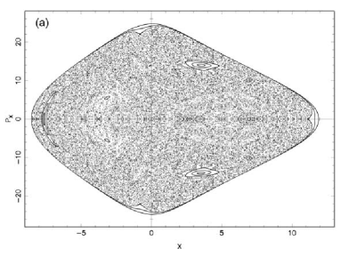
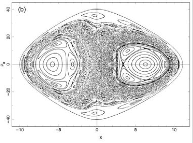
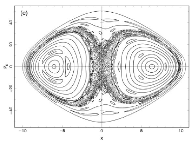
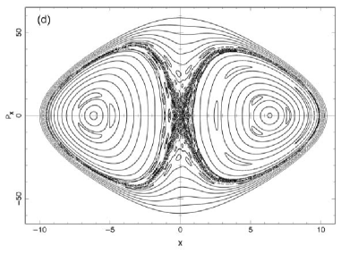
Figure 1: The $(x,p_{x})$ phase plane when (a) $M_{h}=0$, $h_{2}=516$; (b) $M_{h}=10\,000$, $h_{2}=-226$; (c) $M_{h}=20\,000$, $h_{2}=-1007$ and (d) $M_{h}=30\,000$, $h_{2}=-1788$. The values of all other parameters are given in the text.

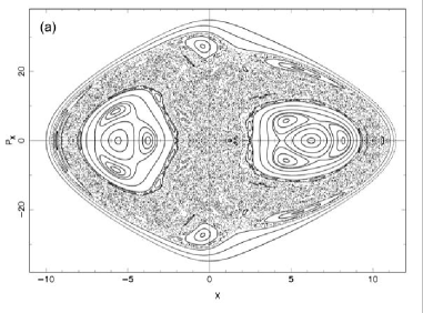
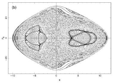
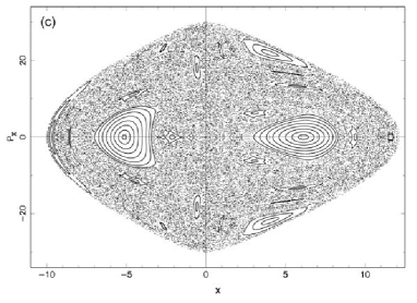
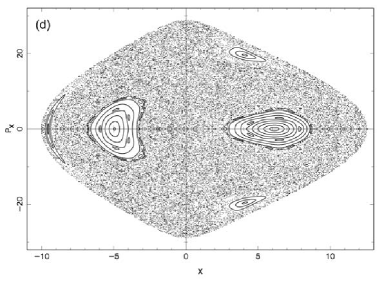
Figure 2: The $(x,p_{x})$ phase plane, when $M_{h}=10\,000$ and (a) $c_{h}=10.5$, $h_{2}=-135$; (b) $c_{h}=13$, $h_{2}=-55$; (c) $c_{h}=15.5$, $h_{2}=11$ and (d) $c_{h}=18$, $h_{2}=68$. The values of all other parameters are given in the text.

Figure 1(a)–(d) shows the $(x,p_{x})$, $\left(y=0,p_{y}>0\right)$ phase plane for four different values of the mass of the halo. The values of all other parameters are $\upsilon_{0}=15$, $c_{b}=2.5$, $\alpha=1.5$, $b=1.8$, $\lambda=0.03$, and $c_{h}=8$. The values of the energy $h_{2}$ were chosen so that in all phase planes $x_{\rm max}\simeq 10$. Figure 1(a) shows the phase plane when the system has no halo component, that is when $M_{h}=0$. The value of $h_{2}$ is 516. One can see that almost all of the phase plane is covered by a chaotic sea. The regular regions consist of a small set of islands produced by secondary resonances. Figure 1(b) shows the phase plane when $M_{h}=10\,000$, while $h_{2}=-226$. As we can see, the majority of the phase plane is covered by chaotic orbits. There are also two considerable regular regions inside the chaotic sea. These belong to invariant curves produced by quasi-periodic orbits which are characteristic of a 1:1 resonance. There are also regular regions produced by quasi-periodic orbits which are characteristic of a 2:3 resonance. In the outer part we can see some regular regions produced by quasi-periodic orbits characteristic of the 2:1 resonance. Some small islands produced by secondary resonances are also embedded in the chaotic sea. Figure 1(c) is similar to Figure 1(a) but when $M_{h}=20\,000$ and $h_{2}=-1007$. Here, the chaotic region is much smaller, while the majority of orbits are regular. The most prominent characteristic of this phase plane is the presence of many small islands produced by secondary resonances. Figure 1(d) shows the phase plane when $M_{h}=30\,000$ and $h_{2}=-1788$. Here we only see a small chaotic layer, while the rest of the phase plane is covered by regular orbits. The characteristic of this phase plane is that a considerable part of the regular orbits are box orbits. Secondary resonances are also observed.

Therefore, our numerical results suggest that the chaotic regions in our 2D composite galactic dynamical system described by the Hamiltonian Equation (8) strongly depend on the mass of the halo component. The mass of the halo acts as a catalyst on the asymmetry of the galaxy and drastically reduces the percentage of the chaotic orbits. Thus, one can conclude that massive spherical dark halos can act as chaos controllers in galaxies showing small asymmetries.

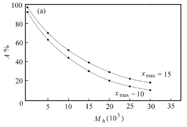
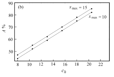
Figure 3: (a) A plot of the area $A\%$ covered by chaotic orbits vs. $M_{h}$ and (b) A plot of the area $A\%$ covered by chaotic orbits vs. $c_{h}$. The values of all the other parameters are given in text.

Figure 2(a)–(d) is similar to Figure 1(a)–(d), when $M_{h}$ is 10 000 while $c_{h}$ is treated as a parameter. All other parameters are as shown in Figure 1. Here again, the values of the energy $h_{2}$ were chosen so that in all phase planes $x_{\rm max}\simeq 10$. In Figure 2(a) we have $c_{h}=10.5$ and $h_{2}=-135$. Here the phase plane has a large chaotic region, while one also observes considerable areas of regular motion. In Figure 2(b), where the values of $c_{h}$ and $h_{2}$ are 13 and –55, respectively, the chaotic sea increases, while the regular region decreases. In the phase plane shown in Figure 2(c), we have taken $c_{h}=15.5$ and $h_{2}=11$. Obviously, the chaotic sea is larger than that shown in Figure 2(b). On the other hand, the regular region is smaller than that given in Figure 2(b). Finally, in the results presented in Figure 2(d) we have chosen $c_{h}=18$ and $h_{2}=68$. Here the chaotic sea is even larger, while the regular regions are smaller than those shown in Figure 2(c).

The conclusion is that, for a given mass of the dark halo component, the percentage of chaotic orbits increases as the scale length of the halo increases. In other words, the numerical experiments indicate that one would expect to observe less chaos in asymmetric triaxial galaxies surrounded by dense halos, while the chaotic orbits would increase in similar galaxies surrounded by less dense spherical halo components.

Figure 3(a) shows the percentage of the phase plane $A\%$ covered by chaotic orbits as a function of the mass of the dark halo, for two different values of $x_{\max}$. The values of the parameters are $\upsilon_{0}=15$, $c_{b}=2.5$, $\alpha=1.5$, $b=1.8$, $\lambda=0.03$ and $c_{h}=8$. We see that $A\%$ decreases exponentially as $M_{h}$ increases. Figure 3(b) shows a plot of $A\%$ and $c_{h}$. The values of the parameters are $\upsilon_{0}=15$, $c_{b}=2.5$, $\alpha=1.5$, $b=1.8$, $\lambda=0.03$ and $M_{h}=10\,000$. Here we see that $A\%$ increases linearly as $c_{h}$ increases. The authors would like to make it clear that $A\%$ is estimated on a completely empirical basis by measuring the area in the $(x,p_{x})$ phase plane occupied by chaotic orbits.

Figure 4(a) and (b) shows a plot of the Lyapunov Characteristic Exponent (LCE) (see Lichtenberg & Lieberman 1992) vs. $M_{h}$ and $c_{h}$, respectively. The values of the parameters for Figure 4(a) are the same as in Figure 3(a) and for Figure 4(b) are the same as in Figure 3(b). One can see, in Figure 4(a), that the LCE decreases exponentially when $M_{h}$ increases, while in Figure 4(b) we see that the LCE increases exponentially when $c_{h}$ increases. Here we must point out that it is well known that the LCE has different values in each chaotic component (see Saitô & Ichimura 1979). Since we have regular regions in all cases and only a large chaotic sea, we calculate the average value of the LCE in each case by taking thirty orbits with different initial conditions in the chaotic sea. In all cases, the calculated values of the LCEs were different in the fourth decimal point in the same chaotic sea.

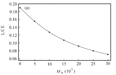
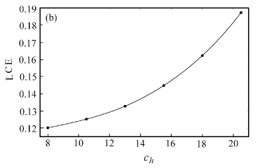
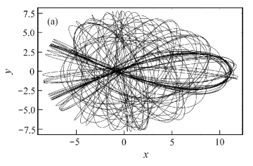
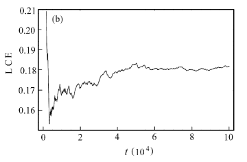
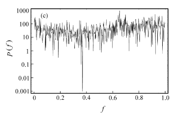
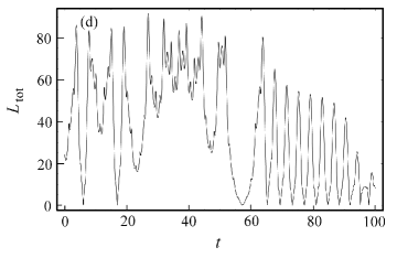
Figure 4: (a) A plot of the LCE vs. $M_{h}$ and (b) A plot of the LCE vs. $c_{h}$. The values of all the other parameters are given in the text.

Figure 5: (a) An orbit in the 2D potential, (b) Corresponding LCE, (c) $P(f)$ indicator and (d) $L_{\rm tot}$ indicator. The motion is chaotic. See text for details.

In the following, we shall investigate the regular or chaotic character of orbits in the 2D Hamiltonian Equation (8) using the new dynamical indicator $L_{\rm tot}$. In order to see the effectiveness of the new method, we shall compare the results with two other indicators, the classical method of the LCE and the method $P(f)$ used by Karanis & Vozikis (2008). This method uses the Fast Fourier Transform (F.F.T.) of a series of time intervals, each one representing the time that elapsed between two successive points on the Poincarè $(x,p_{x})$ phase plane for 2D systems, while for 3D systems they take two successive points on the plane $z=0$.

Figure 5(a) shows an orbit with initial conditions $x_{0}=-1.0$ and $y_{0}=p_{x0}=0$, while the value of $p_{y}$ is always found from the energy integral for all orbits. The values of all other parameters and energy are the same as in Figure 1(a). One observes in Figure 5(b) that the LCE, which was computed for a period of $10^{5}$ time units, has a value of about 0.18, indicating chaotic motion. The same result is shown by the $P(f)$ indicator, which is given in Figure 5(c). Figure 5(d) shows a plot of the $L_{\rm tot}$ vs. time for a time interval of 100 time units. We see that the diagram is highly asymmetric. Furthermore, one observes large deviations between the maxima and also large deviations between the minima in the $[L_{\rm tot},t]$ plot. The above characteristics suggest that the corresponding orbit is chaotic.

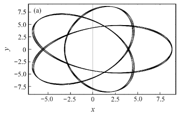
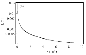
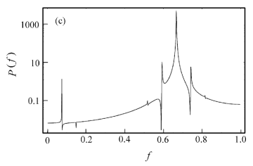
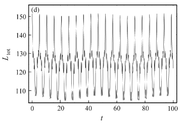
Figure 6: Similar to Fig. 5(a)–(d). The motion is regular.

Figure 6(a) shows an orbit with initial conditions $x_{0}=8.8$ and $y_{0}=p_{x0}=0$. The values of all other parameters and energy are the same as in Figure 1(b). As we can see, this is a quasi-periodic orbit. Therefore the LCE of this orbit goes to zero, as is clearly seen in Figure 6(b). The $P(f)$ indicator in Figure 6(c) shows a small number of peaks, also indicating regular motion. The plot of the $L_{\rm tot}$ given in Figure 6(d) is now quasi-periodic, with symmetric peaks, indicating regular motion.

Figure 7: Similar to Fig. 6(a)–(d) for a regular orbit.

Figure 8: Similar to Fig. 5(a)–(d) for a chaotic orbit.

Figure 7(a)–(d) is similar to Figure 6(a)–(d) for an orbit with initial conditions $x_{0}=-9.36$ and $y_{0}=p_{x0}=0$, while the values of all other parameters and energy are the same as in Figure 2(a). As we can see, the orbit is quasi-periodic and this fact is indicated by all three dynamical parameters. On the contrary, the orbit shown in Figure 8(a) has initial conditions $x_{0}=10$ and $y_{0}=p_{x0}=0$ while the values of all other parameters and energy are the same as in Figure 2(d). The orbit looks chaotic and this is indicated by the LCE, the $P(f)$ and the $L_{\rm tot}$ shown in Figure 8(b), 8(c) and 8(d), respectively.

A large number of orbits in the 2D system were calculated for different values of the parameters. All of the numerical results suggest that the $L_{\rm tot}$ is a fast and reliable dynamical parameter and can be safely used in order to distinguish ordered from chaotic motion. There is no doubt that the $L_{\rm tot}$ method is much faster than the LCE, because it needs only about a hundred time units, while the LCE needs about a hundred thousand time units. The $P(f)$ indicator needs several thousand time units in order to give reliable results. Furthermore, it needs the computation of the phase plane of the system, while the $L_{\rm tot}$ only needs the calculations of the corresponding orbit.

3 The character of motion in the 3D model

We shall now proceed to investigate the regular or chaotic behavior of the orbits in the 3D Hamiltonian Equation (5). The regular or chaotic nature of the 3D orbits is found as follows: We choose initial conditions $\left(x_{0},p_{x0},z_{0}\right)$, $y_{0}=p_{z0}=0$, such that $\left(x_{0},p_{x0}\right)$ is a point on the phase plane of the 2D system. The point $\left(x_{0},p_{x0}\right)$ lies inside the limiting curve

$$\frac{1}{2}p_{x}^{2}+V_{t}(x)=h_{2},$$ (9)

which is the curve containing all the invariant curves of the 2D system. We choose $h_{3}=h_{2}$ and the value of $p_{y0}$, for all orbits, is obtained from the energy integral Equation (5). Our numerical experiments show that orbits with initial conditions $\left(x_{0},p_{x0},z_{0}\right)$, $y_{0}=p_{z0}=0$, such as $\left(x_{0},p_{x0}\right)$ which is a point in the chaotic regions of Figures 1(a)–(d) and 2(a)–(d) for all permissible values of $z_{0}$, produce chaotic orbits.

Our next step is to study the character of orbits with initial conditions $\left(x_{0},p_{x0},z_{0}\right),y_{0}=p_{z0}=0$, such as $\left(x_{0},p_{x0}\right)$ which is a point in the regular regions of Figure 1(a)–(d) and Figure 2(a)–(d). It was found that in all cases the regular or chaotic character of the above 3D orbits depends strongly on the initial value $z_{0}$. Orbits with small values of $z_{0}$ are regular, while for large values of $z_{0}$ they change their character and become chaotic. The general conclusion, which is based on the results derived from a large number of orbits, is that orbits with values of $z_{0}\geq 0.75$ are chaotic, while orbits with values of $z_{0}<0.75$ are regular.

Figure 9(a) shows the LCE of the 3D system, as a function of the mass of the halo, for a large number of chaotic orbits when $c_{h}=8$. The values of the parameters are shown in Figure 4(a). We see that the LCE decreases exponentially as the mass of the halo increases. Figure 9(b) shows the LCE as a function of $c_{h}$ when $M_{h}=10\,000$. The values of the parameters are shown in Figure 4(b). Here the LCE increases exponentially as $c_{h}$ increases. The above results suggest that the degree of chaos decreases in asymmetric triaxial galaxies with more dense and more massive halo components.

Figure 10(a)–(d) is similar to Figure 8(a)–(d) but for a 3D orbit. The orbit shown in Figure 10(a) looks chaotic. Initial conditions are $x_{0}=2.0$, $p_{x0}=0$ and $z_{0}=0.5$. Remember that all orbits have $y_{0}=p_{z0}=0$, while the value of $p_{y0}$ is always found from the energy integral. The values of all other parameters and energy $h_{3}$ are the same as in Figure 2(b). The LCE shown in Figure 10(b) assures the chaotic character of the orbit. The $P(f)$ given in Figure 10(c) also suggests chaotic motion. The same conclusion comes from the $L_{\rm tot}$, which is shown in Figure 10(d). Figure 11(a)–(d) is similar to Figure 10(a)–(d) but for a quasi-periodic 3D orbit. The initial conditions are $x_{0}=5.0$, $p_{x0}=0$ and $z_{0}=0.1$. The values of all other parameters and energy $h_{3}$ are the same as in Figure 1(c). Here one observes that all three detectors support the regular character of orbits.

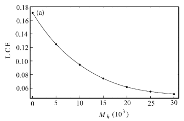
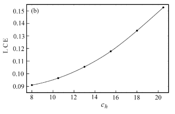
Figure 9: Similar to Fig. 4(a)–(b) for the 3D potential. The values of all other parameters are given in the text.

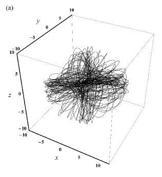
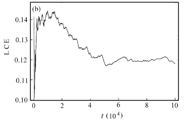
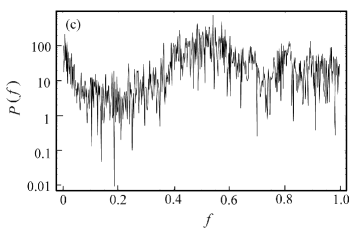
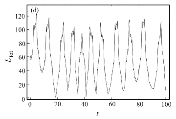
Figure 10: (a) An orbit in the 3D potential, (b) The corresponding LCE, (c) The $P(f)$ indicator and (d) The $L_{\rm tot}$ indicator. The motion is chaotic. See the text for details.

Figure 11: Similar to Fig. 10(a)–(d). The motion is regular.

Figure 12: (a) A 3D chaotic orbit and (b) The corresponding $L_{\rm tot}$. See text for details.

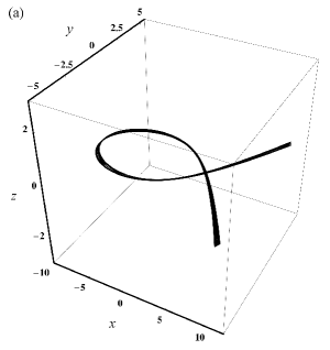
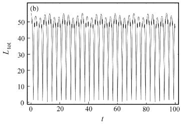
Figure 13: Similar to Fig. 12(a)–(b) for a quasi-periodic orbit.

Two more examples of 3D orbits are given in Figure 12(a) and (b) and Figure 13(a) and (b). Here we present only the orbit and the $L_{\rm tot}$. In Figure 12(a) and (b) the orbit has initial conditions $x_{0}=-1.0$, $p_{x0}=0$ and $z_{0}=0.5$. The values of all other parameters and energy $h_{3}$ are shown in Figure 2(c). The motion is chaotic. In Figures 13(a) and (b) the orbit has initial conditions $x_{0}=-9.55$, $p_{x0}=0$ and $z_{0}=0.1$. The values of all other parameters and energy $h_{3}$ are as shown in Figure 2(d). The motion is regular.

The main conclusion for the study of the 3D model is that the $L_{\rm tot}$ indicator can give reliable and very fast results for the character of the orbits. There is no doubt that the $L_{\rm tot}$ is much faster than the two other indicators used in this research. Therefore, we can say that this indicator is a very useful tool for a quick study of the character of orbits in galactic potentials.

4 Discussion and conclusions

In this article, we have studied the regular and chaotic character of motion in a 3D galactic potential. The potential describes the motion in a triaxial elliptical galaxy with a small asymmetry surrounded by a dark halo component. Dark halos may have a variety of shapes (see Ioka et al. 2000; Olling & Merrifield 2000; Oppenheimer et al. 2001; McLin et al. 2002; Penton et al. 2002; Steidel et al. 2002; Wechsler et al. 2002; Papadopoulos & Caranicolas 2006; Caranicolas & Zotos 2010). In this investigation we have used a spherical dark halo component.

In order to distinguish between regular and chaotic motion, we have introduced and used a new fast indicator, the $L_{\rm tot}$. The validity of the results given by the new indicator was checked using the LCE and an earlier method used by Karanis & Vozikis (2008). We started from the 2D system and then extended the results to the 3D potential.

The main conclusions of this research are the following:

• The percentage of chaotic orbits decreases as the mass of the spherical halo increases. Therefore, the mass of the halo can be considered as an important physical quantity, acting as a controller of chaos in galaxies showing small asymmetries.

• We expect to observe a smaller fraction of chaotic orbits in asymmetric triaxial galaxies with a dense spherical halo, while the fraction of chaotic orbits would increase in asymmetric triaxial galaxies surrounded by less dense spherical halo components.

• It was found that the LCE in both the 2D and the 3D models decreases as the mass of the halo increases, while the LCE increases as the scale length $c_{h}$ of the halo increases. This means that not only the percentage of chaotic orbits, but also the degree of chaos is affected by the mass or the scale length of the spherical halo component.

• The $L_{\rm tot}$ gives fast and reliable results regarding the nature of motion, both in 2D and 3D galactic potentials. For all calculated orbits, the results given by the $L_{\rm tot}$ coincide with the outcomes obtained using the LCE or the $P(f)$ method used by Karanis & Vozikis (2008). The advantage of the $L_{\rm tot}$ is that it is faster than the above two methods.