Abstract

The corner polyhedron is described by minimal valid inequalities from maximal lattice-free convex sets. For the Relaxed Corner Polyhedron (RCP) with two free integer variables and any number of non-negative continuous variables, it is known that such facet defining inequalities arise from maximal lattice-free splits, triangles and quadrilaterals. We improve on the tightest known upper bound for the approximation of the RCP, purely by minimal valid inequalities from maximal lattice-free quadrilaterals, from 2 to 1.71. We generalize the tightest known lower bound of 1.125 for the approximation of the RCP, purely by minimal valid inequalities from maximal lattice-free triangles, to an infinite subclass of quadrilaterals.

1 Introduction

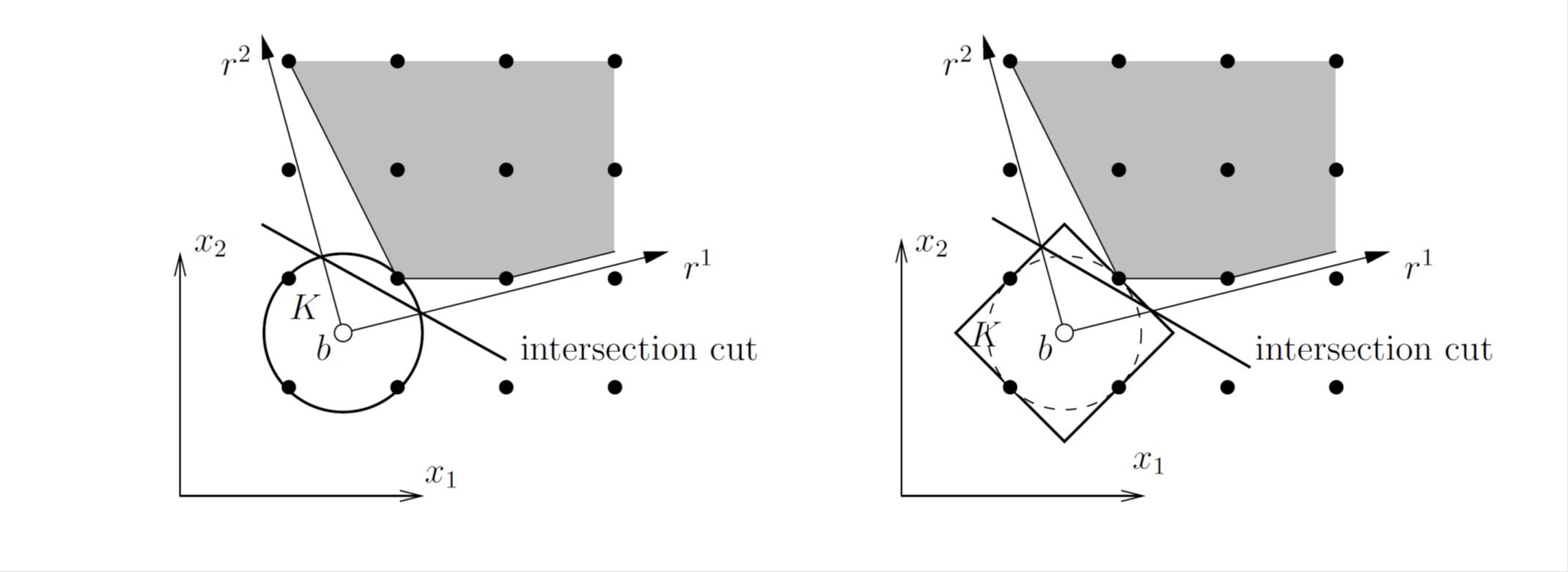
Figure 1: Correspondence between intersection cuts and facets of the corner polyhedron. (Cornuéjols et al. [6]).

Corner polyhedra, introduced by Gomory [11], are obtained by relaxing the non-negativity restrictions on the set of basic variables of a mixed-integer linear program (MILP). This means we can drop the constraints for all continuous basic variables. Any inequality valid for the corner polyhedron is valid for the original polyhedron. Moreover, the set of nontrivial facets of the corner polyhedron is the same (see Figure 1 for intuition) as the set of undominated intersection cuts (Cornuéjols et al. [6]). The recent paper by Andersen et al. [1] has led to a renewed interest in corner polyhedra as a tool to generate stronger multi-row cuts as opposed to traditional single-row cuts. The interested reader may refer to Cornuéjols et al. [6] for a comprehensive review of corner polyhedra.

We consider the problem in Andersen et al. [1] , which has two integer constrained basic variables and any number of nonbasic nonzero continuous variables i.e. MILP: $x=f+\sum_{j=1}^{k}r_{j}s_{j},f\in\mathbb{Q}^{2}\setminus\mathbb{Z}^{2},k\geq 1,x\in\mathbb{Z}^{2},s\in\mathbb{R}_{+}^{k}$. We define $R_{f}(r_{1},\dots,r_{k})=\text{Conv}(s\in\mathbb{R}_{+}^{k}:f+\sum_{j=1}^{k}r_{j}s_{j}\in\mathbb{Z}^{2})$. It is important to note that the traditional Gomory corner polyhedron with two free integer basic variables would allow for both continuous and discrete nonbasic variables, whereas the above formulation allows only for continuous nonbasic variables. Hence, we call $R_{f}(r_{1},\dots,r_{k})$ the Relaxed Corner Polyhedron (RCP), following the notation of Basu et al. [3]. It is useful to consider the semi-infinite relaxation given by $R_{f}=\text{Conv}(s\in\mathbb{R}_{+}^{\infty}:f+\sum_{r\in\mathbb{Q}^{2}}rs_{r}\in\mathbb{Z}^{2})$ because the minimal valid inequalities for $R_{f}$ are known in terms of the minimal valid functions (a.k.a. gauge functions) of maximal lattice-free convex sets containing $f$ in their interior. Any maximal lattice-free (MLF) convex set $B$ defines a minimal valid function $\psi_{B}:\mathbb{R}^{2}\rightarrow\mathbb{R}_{+}$ such that $\psi_{B}(0)=0$ and $\psi_{B}(x-f)=1$ $\forall x\in\text{Boundary}(B)$. If $\exists\lambda\geq 0$ s.t. $f+\lambda r\in\text{Boundary}(B)$, then $\psi_{B}(r)=1/\lambda$ else $\psi_{B}(r)=0$. $R_{f}=\bigcap_{B}(\sum_{r\in\mathbb{Q}^{2}}\psi_{B}(r)s_{r}\geq 1)$. A restriction of these infinite dimensional minimal valid functions to the set of extreme rays of the RCP gives minimal valid functions for the finite dimensional RCP i.e. $R_{f}(r_{1},\dots,r_{k})=\bigcap_{B}(\sum_{j=1}^{k}\psi_{B}(r_{j})s_{j}\geq 1)$ (Borozan and Cornuéjols [5]). Theorems 1.1, 1.2 and 1.3 encapsulate some key properties of maximal lattice-free convex sets.

Theorem 1.1.

(Doignon [9], Bell [4] and Scarf [13]): Any full dimensional maximal lattice-free convex set $K\subseteq\mathbb{R}^{p}$ has at most $2^{p}$ facets.

Theorem 1.2.

(Lovász [12]): In the plane, a maximal lattice-free convex set with a nonempty interior is one of the following:
i) A split $c\leq ax_{1}+bx_{2}\leq c+1$ where $a$, $b$ are coprime, $c$ is an integer,
ii) A triangle with an integral point in the interior of each of its edges,
iii) A quadrilateral containing exactly four integral points, with exactly one of them in the interior of each of its edges.

Figure 2 shows the three types of maximal lattice-free convex sets.

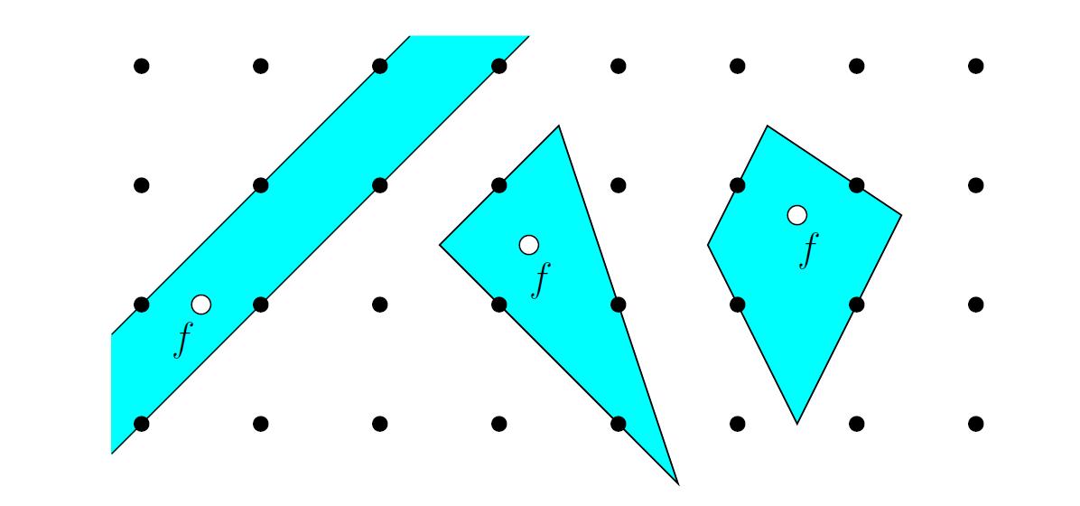
Figure 2: Maximal lattice-free convex sets with nonempty interior in $\mathbb{R}^{2}\hskip 4.0pt$(Cornuéjols et al. [6]).

Theorem 1.3.

(Dey and Wolsey [8]) The maximal lattice-free triangles are of three types:
(i) Type-1 triangles: triangles with integral vertices and exactly one integral point in the relative interior of each edge,
(ii) Type-2 triangles: triangles with at least one fractional vertex v, exactly one integral point in the relative interior of the two edges incident to v and at least two integral points on the third edge,
(iii) Type-3 triangles: triangles with exactly three integral points on the boundary, one in the relative interior of each edge.

Figure 3 shows the three types of maximal lattice-free triangles.

We define the split closure $S_{f}(r_{1},\dots,r_{k})$, triangle closure $T_{f}(r_{1},\dots,r_{k})$ and quadrilateral closure $Q_{f}(r_{1},\dots,r_{k})$ as follows.

$$S_{f}(r_{1},\dots,r_{k})\hskip 4.0pt=\bigcap_{B:B\hskip 4.0ptis\hskip 4.0pta\hskip 4.0ptmaximal\hskip 4.0ptlattice-free\hskip 4.0ptsplit}(\hskip 4.0pt\sum_{j=1}^{k}\psi_{B}(r_{j})s_{j}\geq 1).$$ (1)

$$T_{f}(r_{1},\dots,r_{k})\hskip 4.0pt=\bigcap_{B:B\hskip 4.0ptis\hskip 4.0pta\hskip 4.0ptmaximal\hskip 4.0ptlattice-free\hskip 4.0pttriangle}(\hskip 4.0pt\sum_{j=1}^{k}\psi_{B}(r_{j})s_{j}\geq 1).$$ (2)

$$Q_{f}(r_{1},\dots,r_{k})\hskip 4.0pt=\bigcap_{B:B\hskip 4.0ptis\hskip 4.0pta\hskip 4.0ptmaximal\hskip 4.0ptlattice-free\hskip 4.0ptquadrilateral}(\hskip 4.0pt\sum_{j=1}^{k}\psi_{B}(r_{j})s_{j}\geq 1).$$ (3)

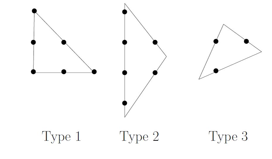
Figure 3: Three types of maximal lattice-free triangles (Cornuéjols et al. [6]).

Theorem 1.2 gives us the following result.

Theorem 1.4.

$R_{f}(r_{1},\dots,r_{k})=S_{f}(r_{1},\dots,r_{k})\cap T_{f}(r_{1},\dots,r_{k})\cap Q_{f}(r_{1},\dots,r_{k})$.

It is easy to see that maximal lattice-free splits are a limiting case of maximal lattice-free triangles, quadrilaterals. The following theorems follow (see Basu et al. [2] for a rigorous proof).

Theorem 1.5.

(Basu et al. [2]): $T_{f}(r_{1},\dots,r_{k})\subseteq S_{f}(r_{1},\dots,r_{k}),Q_{f}(r_{1},\dots,r_{k})\subseteq S_{f}(r_{1},\dots,r_{k})$.

Theorem 1.6.

(Basu et al. [2]) $R_{f}(r_{1},\dots,r_{k})=T_{f}(r_{1},\dots,r_{k})\cap Q_{f}(r_{1},\dots,r_{k})$.

It is important to note that if we ignore maximality and consider all triangles and quadrilaterals, then the set of triangles is redundant and the RCP can be defined just in terms of quadrilaterals. This is because each triangle can be approximated arbitrarily closely by a sequence of quadrilaterals. However, a maximal lattice-free Type-3 triangle cannot be approximated (see Figure 4) arbitrarily closely by a sequence of maximal lattice-free quadrilaterals. Hence, considering only maximal sets, we need both maximal lattice-free triangles and quadrilaterals.

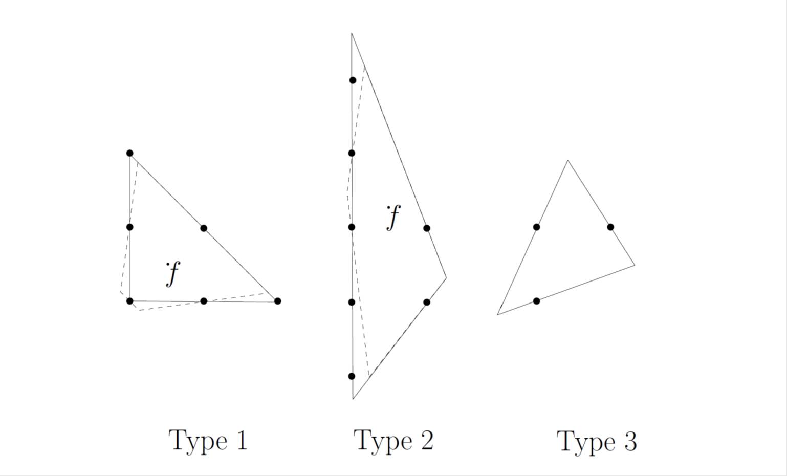
Figure 4: Type-3 maximal lattice-free triangles cannot be approximated by maximal lattice-free quadrilaterals (Basu et al. [2]).

2 Our Contribution

In Section 3, we address the problem of determining how well the quadrilateral closure approximates the RCP. This amounts to finding the smallest possible value $\alpha_{Q}$ of the parameter $\alpha\geq 1$ such that $R_{f}(r_{1},\dots,r_{k})\subseteq Q_{f}(r_{1},\dots,r_{k})\subseteq\alpha R_{f}(r_{1},\dots,r_{k})$. To the best of our knowledge, the tightest upper bound - published or unpublished, of 2, appears in Basu et al. [2] i.e. we know that $\alpha_{Q}\leq 2$. We improve this bound from 2 to 1.71.

In Section 4, we take up the problem of approximation of the RCP by the triangle closure. This means finding the smallest possible value $\alpha_{T}$ of the parameter $\alpha\geq 1$ such that $R_{f}(r_{1},\dots,r_{k})\subseteq T_{f}(r_{1},\dots,r_{k})\subseteq\alpha R_{f}(r_{1},\dots,r_{k})$. To the best of our knowledge, the tightest lower bound - published or unpublished, of 1.125, appears in Cornuéjols et al. [7] i.e. we know that $\alpha_{T}\geq 1.125$. In Section 4, we generalize this lower bound of 1.125 to an infinite subclass of quadrilaterals.

3 Upper bound for approximation of the RCP by the quadrilateral closure

In this section, we address the problem of finding the tightest possible upper bound $\alpha_{Q}$ for approximation of the RCP by the quadrilateral closure.

3.1 Existing state-of-the-art bound of 2

The current tightest upper bound, which is from Basu et al. [2] is 2, meaning $\alpha_{Q}\leq 2$. We summarize here the theoretical tools which were used and which we will borrow from this work as well. We also introduce some new notation, which is more compact, for our analysis. An elegant tool used in the analysis is Goemans theorem.

Theorem 3.1.

(Goemans [10]): Let $A\subseteq\mathbb{R}^{n}_{+}\setminus\{0\}$ be a polyhedron of the form $A=\{x:a^{i}x\geq b_{i}\hskip 4.0pt\forall i=1,\dots,m\}$ where $a^{i}\geq 0$ and $b^{i}\geq 0\hskip 4.0pt\forall i=1,\dots,m$. Let $\alpha>0$ be a scalar. Define $\alpha A=\{x:\alpha a^{i}x\geq b^{i}\hskip 4.0pt\forall i=1,\dots,m\}.$ If the convex set $B$ is a relaxation of $A$, then the smallest $\alpha\geq 1$ such that $B\subseteq\alpha A$ is given by

$$\max_{i=1,\dots,m}\{{{\frac{b_{i}}{\inf\{\large a^{i}x:x\in B\}}}:\large b_{i}>0\}}.$$

The above theorem implies that we need to optimize along the direction of each facet-defining inequality of the polyhedron to be approximated while remaining within the convex set used for approximation and take the best amongst such optimals. To determine how well the quadrilateral closure approximates the RCP, we need to obtain

$$\inf\limits_{\text{(}f\text{, MLF set }B\text{): }\psi_{B}^{f}\text{ defines a facet of }R_{f}}\inf\limits_{\large s}\{\sum_{i=1}^{k}\psi_{B}^{f}(r_{i})s_{i}:s\in Q_{f}(r_{1},\dots,r_{k})\}.$$ (4)

If a facet defining inequality arises from a maximal lattice-free quadrilateral, then its contribution to the maximization term in Theorem 3.1 cannot exceed 1. Hence, only facet-defining inequalities from maximal lattice-free triangles need to be considered. i.e.

$$\inf\limits_{\text{(}f\text{, MLF set }B\text{): }\psi_{B}^{f}\text{ defines a facet of }R_{f}}\text{ }\inf\limits_{s}\{\sum_{i=1}^{k}\psi_{B}^{f}(r_{i})s_{i}:s\in Q_{f}(r_{1},\dots,r_{k})\}$$

$$=\inf\limits_{\text{(}f\text{, MLF triangle }T\text{): }\psi_{T}^{f}\text{ defines a facet of }R_{f}}\text{ }\inf\limits_{s}\{\sum_{i=1}^{k}\psi_{T}^{f}(r_{i})s_{i}:s\in Q_{f}(r_{1},\dots,r_{k})\}.$$ (5)

However, we know that (see Figure 4) Type-2 triangles can be approximated arbitrarily closely by maximal lattice-free quadrilaterals (Basu et al. [2]). Also, Type-1 triangles can be approximated arbitrarily closely by Type-2 triangles and thus by maximal lattice-free quadrilaterals. Hence, we need only consider Type-3 triangles i.e.

$$\inf\limits_{\text{(}f\text{, MLF triangle }T\text{): }\psi_{T}^{f}\text{ defines a facet of }R_{f}}\text{ }\inf\limits_{s}\{\sum_{i=1}^{k}\psi_{T}^{f}(r_{i})s_{i}:s\in Q_{f}(r_{1},\dots,r_{k})\}$$ (6)

$$=\inf\limits_{\text{(}f\text{, Type-3 MLF triangle }T\text{): }\psi_{T}^{f}\text{ defines a facet of }R_{f}}\inf\limits_{s}\{\sum_{i=1}^{k}\psi_{T}^{f}(r_{i})s_{i}:s\in Q_{f}(r_{1},\dots,r_{k})\}.$$ (7)

Basu et al. [2] use the positive homogeneity of $\psi$ and that $\psi$ is unity for all points on the boundary of T (with shift of origin to $f$). When $\psi_{B}(r_{j})>0$, we define $r_{j}$ such that that $f+r_{j}$ is on the boundary of T. This can be done with the requisite scaling, as it does not change the optimal value of $\inf\limits_{s}\{\sum_{i=1}^{k}\psi_{T}^{f}(r_{i})s_{i}:s\in Q_{f}(r_{1},\dots,r_{k})\}$. Thus from now on, we analyze the LP $\inf\limits_{s}\{\sum_{i=1}^{k}s_{i}:s\in Q_{f}(r_{1},\dots,r_{k})\}$.

The following theorem indicates that we only need to consider the corner rays in our analysis.

Theorem 3.2.

(Basu et al. [2]): Let $B_{1},\dots,B_{m}$ be lattice-free convex sets with $f$ in the interior of $B_{p}$, $p=1,\dots,m.$ Let $R_{c}\subseteq\{1,\dots,k\}$ be a subset of the ray indices such that for every ray $r_{j}$ with $j\notin R_{c},r^{j}$ is the convex combination of some two rays in $R_{c}$. Then $(\min$ $\sum_{i=1}^{k}s_{i}\hskip 4.0pt:\hskip 4.0pt\sum_{i=1}^{k}\psi_{B_{p}}(r_{i})s_{i}\geq 1\hskip 4.0pt\forall p=1,\dots m\hskip 4.0pt,s\geq 0)$ $=(\min$ $\sum_{i\in R_{c}}s_{i}\hskip 4.0pt:\hskip 4.0pt\sum_{i\in R_{c}}\psi_{B_{p}}(r_{i})s_{i}\geq 1\hskip 4.0pt\forall p=1,\dots m\hskip 4.0pt,s\geq 0)$.

Thus if $r_{1},\dots,r_{3}$ are the corner rays of a maximal lattice-free triangle $T$, then

$$\inf\limits_{s}\{\sum_{i=1}^{k}s_{i}:s\in Q_{f}(r_{1},\dots,r_{k})\}=\inf\limits_{s}\{\sum_{i=1}^{3}s_{i}:s\in Q_{f}(r_{1},\dots,r_{k})\}.$$ (8)

To prove $\alpha_{Q}\leq 2$, Basu et al. [2] consider a relaxation, say $Rel_{1}(Q_{f}(r_{1},\dots,r_{k}))$ of $Q_{f}(r_{1},\dots,r_{k})$, using just two Type-2 triangles - namely $T_{1}$ and $T_{2}$ (see Figure 5). An affine transformation enables us to consider a tilted co-ordinate system, as shown in Figure 5. The Type-3 triangle (say $T$) is defined by the vertices $f+r_{1}$, $f+r_{2}$ and $f+r_{3}$. $T_{1}$ is given by the side of the Type-3 triangle passing through (0,0), the side of the Type-3 triangle passing through (0,1) and the line $x_{1}=1$. $T_{2}$ is given by the side of the Type-3 triangle passing through (0,0), the side of the Type-3 triangle passing through (1,0) and the line $x_{2}=1$. Basu et al. [2] prove the following theorem for the relaxation.

Theorem 3.3.

Let $T$ be a triangle of Type-3 with corresponding minimal function $\psi$ and generating a facet $\sum_{i=1}^{k}\psi_{T}(r_{i})s_{i}\geq 1$ of $R_{f}(r_{1},\dots,r_{k})$. Then $\inf\{\sum_{i=1}^{k}\psi_{T}(r_{i})s_{i}:s\in Rel_{1}(Q_{f}(r_{1},\dots,r_{k}))\}\geq\frac{1}{2}.$

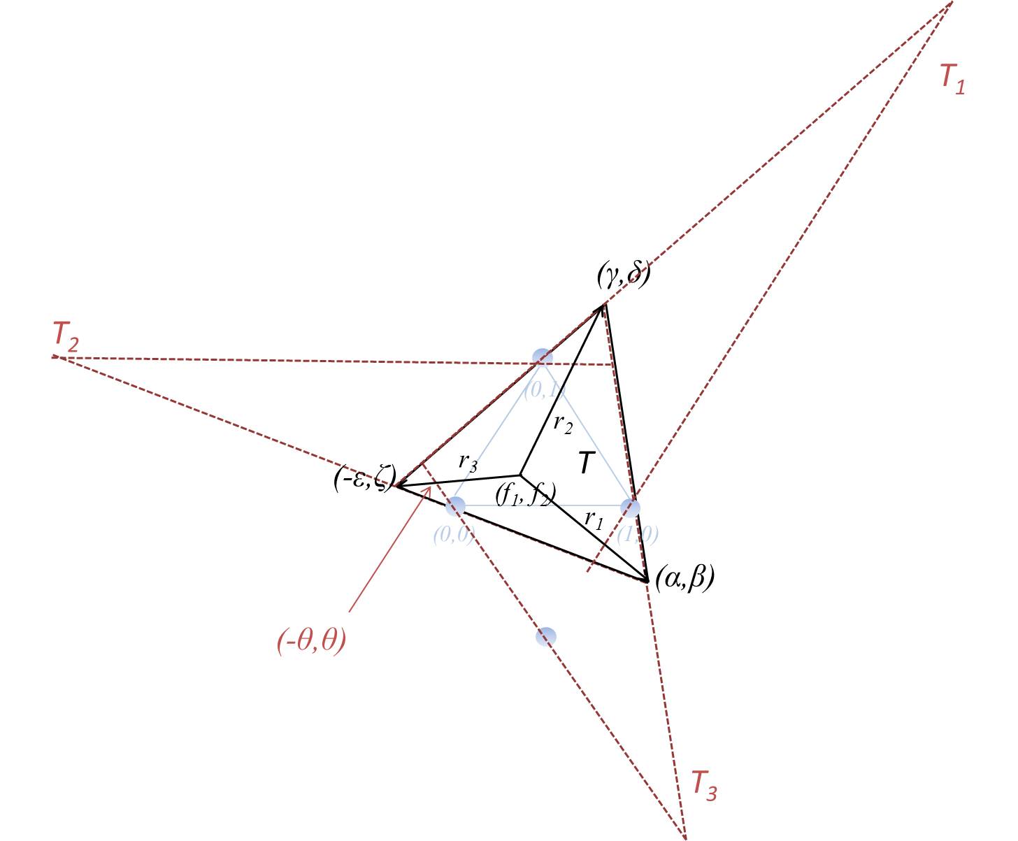
Figure 5: Using three instead of two triangles for the relaxation of the quadrilateral closure gives us an improved bound.

An important result used in the analysis is the following.

Theorem 3.4.

(Basu et al. [2]) Let $\mathcal{F}$ be the family of triangles formed by three lines given by

$$Line\text{ 1 }:-\frac{x_{1}}{t_{1}}+x_{2}=1\text{ with }0<t_{1}<\infty;$$

$$Line\text{ 2 }:t_{2}x_{1}+x_{2}=0\text{ with }0<t_{2}<1;$$

$$Line\text{ 3 }:x_{1}+\frac{x_{2}}{t_{3}}=1\text{ with }1<t_{3}<\infty.$$ (9)

Any Type-3 triangle is either a triangle from $\mathcal{F}$ or the reflection of a triangle from $\mathcal{F}$ about the line $x_{1}=x_{2}$.

Thus, by reflexive symmetry, it suffices to consider the family of triangles $\mathcal{F}$.

Using rotational symmetry, Basu et al. [2] break the analysis into two cases:
Case (i): $f_{1}\leq\frac{1}{2}$, $f_{2}\leq\frac{1}{2}$.
Case (ii): $f_{1}<0$, $f_{1}+f_{2}\leq\frac{1}{2}$.
For any Type-3 triangle $T$, they show that $\inf\{\sum_{i=1}^{k}\psi_{T}(r_{i})s_{i}:s\in Rel_{1}(Q_{f}(r_{1},\dots,r_{k}))\}\geq\frac{1}{2}$ for Case (i) and $\inf\{\sum_{i=1}^{k}\psi_{T}(r_{i})s_{i}:s\in Rel_{1}(Q_{f}(r_{1},\dots,r_{k}))\}\geq 0.586$ for Case (ii). This gives an overall minimum of 0.5 and thus a bound of 2. The interested reader may refer to Basu et al. [2] for the details.

3.2 Our Improved Bound of 1.71

We improve the existing bound using an additional triangle, namely $T_{3}$ (see Figure 5) instead of just $T_{1},T_{2}$ in the LP relaxation. $T_{3}$ is given by the side of the Type-3 triangle passing through (0,1), the side of the Type-3 triangle passing through (1,0) and the line $x_{1}+x_{2}=0$. Let the relaxation obtained be $Rel_{2}(Q_{f}(r_{1},\dots,r_{k}))$. We prove the following theorem which gives us our improved bound.

Theorem 3.5.

$$\inf\limits_{\text{(}f\text{, Type-3 MLF triangle }T\text{): }\psi_{T}^{f}\text{ defines a facet of }R_{f}}\inf\limits_{s}\{\sum_{i=1}^{3}\psi_{T}^{f}(r_{i})s_{i}:s\in Q_{f}(r_{1},\dots,r_{k})\}\geq 0.586$$ (10)

Corollary 3.6.

$Q_{f}(r_{1},\dots,r_{k})\subseteq 1.71R_{f}(r_{1},\dots,r_{k})$.

Proof of Theorem 10

We divide the proof into two cases, depending on the position of the fractional solution (see Figure 6) .
Case 1: The region (bounded in solid green in Figure 6) in the Type-3 triangle common to all the three Type-2 triangles, namely $T_{1}$, $T_{2}$ and $T_{3}$.
Case 2: the region in the Type-3 triangle lying in exactly two of the three Type-2 triangles.

Case 2: The following result follows easily.

Lemma 3.7.

Let $f$ belong to the region in a Type-3 triangle lying in exactly two of the three Type-2 triangles used for approximation. Then

$$\inf\limits_{\text{(}f\text{, Type-3 MLF triangle }T\text{): }\psi_{T}^{f}\text{ defines a facet of }R_{f}}\inf\limits_{s}\{\sum_{i=1}^{3}\psi_{T}^{f}(r_{i})s_{i}:s\in Q_{f}(r_{1},\dots,r_{k})\}\geq 0.586.$$

Proof.

The region defined by our Case 2 is contained in the region defined by Case (ii) in Basu et al. [2] for which a minimum of 0.586 is known. The result follows. ∎

Case 1: We now prove a result for Case 1, which gives us the improved bound.

Lemma 3.8.

Let $f$ belong to the region in a Type-3 triangle lying in all three of the Type-2 triangles used for approximation. Then

$$\inf\limits_{\text{(}f\text{, Type-3 MLF triangle }T\text{): }\psi_{T}^{f}\text{ defines a facet of }R_{f}}\inf\limits_{s}\{\sum_{i=1}^{3}\psi_{T}^{f}(r_{i})s_{i}:s\in Rel_{2}(Q_{f}(r_{1},\dots,r_{k}))\}\geq 0.633.$$

Proof.

The minimization problem $\inf\limits_{s}\{\sum_{i=1}^{3}\psi_{T}^{f}(r_{i})s_{i}:s\in Rel_{2}(Q_{f}(r_{1},\dots,r_{k}))\}$ is the same as the LP

$$\min\hskip 4.0pt\sum_{i=1}^{3}s_{i}\hskip 4.0pts.t.$$

$$\frac{\alpha-f_{1}}{1-f_{1}}s_{1}+s_{2}+s_{3}\geq 1,$$

$$s_{1}+\frac{\delta-f_{2}}{1-f_{2}}s_{2}+s_{3}\geq 1,$$ (11)

$$s_{1}+s_{2}+\frac{\epsilon+f_{1}}{\theta+f_{1}}s_{3}\geq 1,$$

$$s\in\mathbb{R}^{3}_{+}.$$

The dual of this LP is given by

$$\max\hskip 4.0pt\sum_{i=1}^{3}w_{i}\hskip 4.0pts.t.$$

$$\frac{\alpha-f_{1}}{1-f_{1}}w_{1}+w_{2}+w_{3}\leq 1,$$ (12)

$$w_{1}+\frac{\delta-f_{2}}{1-f_{2}}w_{2}+w_{3}\leq 1,$$

$$w_{1}+w_{2}+\frac{\epsilon+f_{1}}{\theta+f_{1}}w_{3}\leq 1,$$

$$w\in\mathbb{R}^{3}_{+}.$$

The dual optimal solution is given by solving

$$\frac{\alpha-f_{1}}{1-f_{1}}w_{1}+w_{2}+w_{3}=1,$$ (13)

$$w_{1}+\frac{\delta-f_{2}}{1-f_{2}}w_{2}+w_{3}=1,$$

$$w_{1}+w_{2}+\frac{\epsilon+f_{1}}{\theta+f_{1}}w_{3}=1.$$

Let

$$1+a=\frac{\alpha-f_{1}}{1-f_{1}},1+b=\frac{\delta-f_{2}}{1-f_{2}},1+c=\frac{\epsilon+f_{1}}{\theta+f_{1}}.$$ (14)

where $a>0,b>0,c>0,d>0$. Then this system of equations is of the form

$$(1+a)w_{1}+w_{2}+w_{3}=1,$$

$$w_{1}+(1+b)w_{2}+w_{3}=1,$$ (15)

$$w_{1}+w_{2}+(1+c)w_{3}=1.$$

Solving this system of equations gives the optimal objective function value as

$$w_{1}+w_{2}+w_{3}=1-\Bigg{(}\dfrac{1}{1+\dfrac{1}{a}+\dfrac{1}{b}+\dfrac{1}{c}}\Bigg{)}.$$ (16)

We have that

$$\dfrac{1}{a}+\dfrac{1}{b}+\dfrac{1}{c}=\dfrac{1-f_{1}}{\alpha-1}+\dfrac{1-f_{2}}{\delta-1}+\dfrac{\theta+f_{1}}{\epsilon-\theta}.$$ (17)

Firstly, it is worth noting that the denominator of each term is simply the distance of a corner point of the Type-3 triangle from the point of intersection of the side of the corresponding Type-2 triangle (which cuts off a part of the Type 3 triangle including the corner point) and the corner ray from the fractional solution to the corner point. The numerator is the distance of the fractional solution $f$ from this intersection point. Let the slope of the line joining $(\alpha,\beta)$ and $(\gamma,\delta)$ be $-u$, line joining $(\gamma,\delta)$ and $(-\epsilon,\zeta)$ be $w$, line joining $(-\epsilon,\zeta)$ and $(\alpha,\beta)$ be $-v$. From Theorem 3.4 , it follows that $u>1$, $,0<v<1$ and $w>0$.

Lemma 3.9.

$$\dfrac{1-f_{1}}{\alpha-1}+\dfrac{1-f_{2}}{\delta-1}+\dfrac{\theta+f_{1}}{\epsilon-\theta}=\\ (1-f_{1})(\frac{u}{v}-1)+(1-f_{2})\dfrac{u+w}{w(u-1)}+\dfrac{(f_{1}+f_{2})(v+w)}{1-v}.$$ (18)

Proof.

See Appendix A.1. ∎

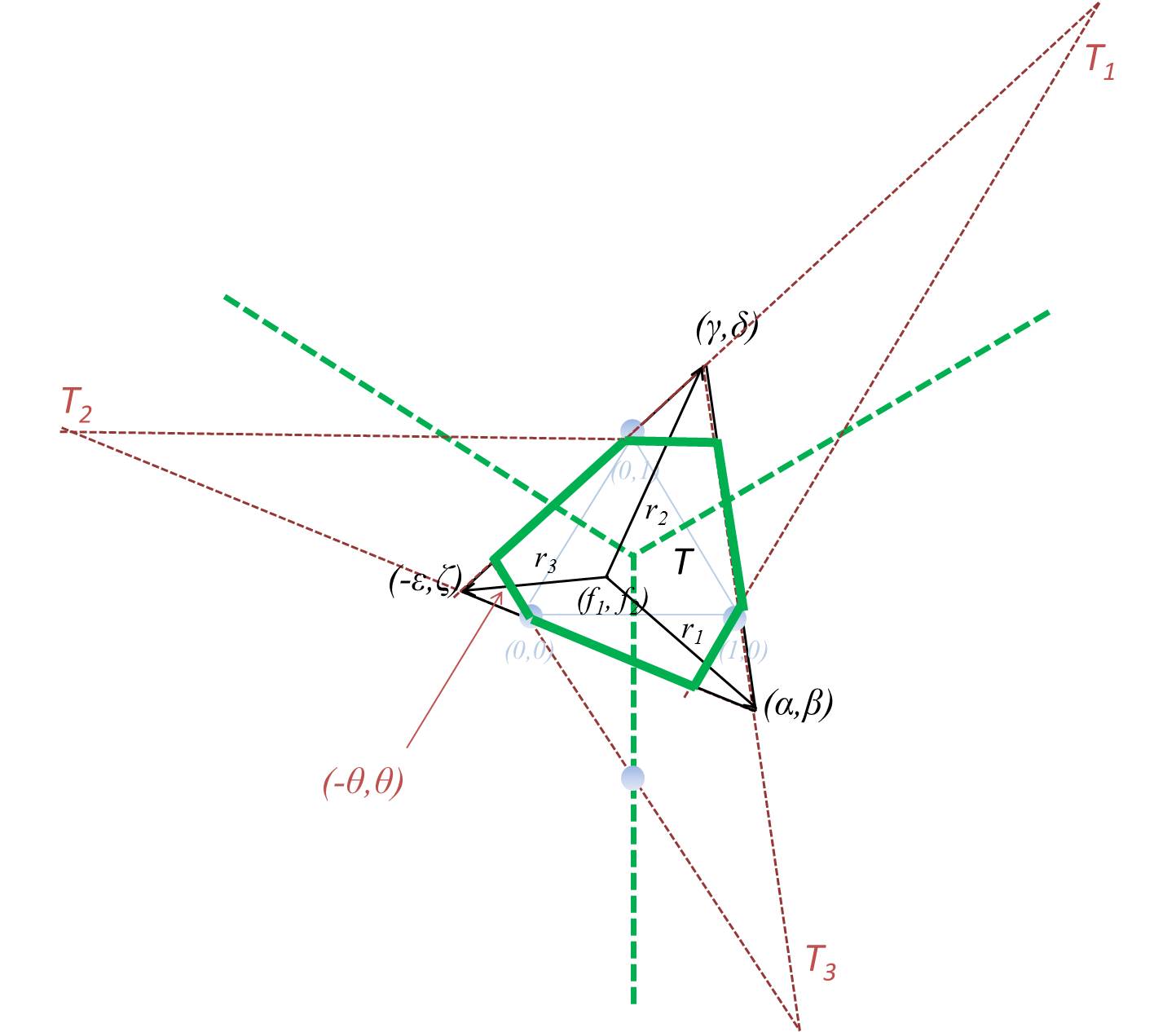
Figure 6: Breakup of cases in our analysis.

We prove the following result which gives us Theorem 10 and hence the improved bound.

Lemma 3.10.

Let $f$ belong to the region in a Type-3 triangle lying in all three of the Type-2 triangles used for approximation. Then

$$\dfrac{1-f_{1}}{\alpha-1}+\dfrac{1-f_{2}}{\delta-1}+\dfrac{\theta+f_{1}}{\epsilon-\theta}\geq\sqrt{3}.$$

Proof.

Case 1 is given by the region bounded by six lines i.e. i.e. $x_{2}\leq wx_{1}+1$, $x_{2}\leq 1$, $x_{2}\leq-u(x_{1}-1)$, $x_{1}\leq 1$, $x_{2}\geq-vx_{1}$ and $x_{2}\geq-x_{1}$. By rotational symmetry (see the dotted green lines in Figure 6), it suffices to examine the region, say $Q$, given by $x_{1}\leq\dfrac{1}{2}$, $x_{2}\geq-vx_{1}$, $x_{2}\geq-x_{1}$, $x_{2}\leq wx_{1}+1$ and $x_{2}\leq-\dfrac{1}{2}(x_{1}-1)$. This region $Q$ after rotations by 120 degrees and 240 degrees covers the whole Type-3 triangle.

∎

This gives us Lemma 3.8. ∎

Lemmas 3.7 and 3.8 give us Theorem 10. ∎

4 Generalization of the lower bound for the approximation of RCP by the triangle closure

In this section, we address the problem of finding a lower bound on the approximation parameter $\alpha_{T}$ for the approximation of the RCP by the triangle closure. To achieve this, we attempt to find a point in the triangle closure which requires the largest scaling for a valid inequality (of the RCP) defined by a maximal lattice-free quadrilateral such that the point then satisfies the scaled inequality. The best bound known to us in literature - published or unpublished, is due to Cornuéjols et al. [7] and is 1.125, meaning $\alpha_{T}\geq 1.125$. The maximal lattice-free quadrilateral (say Q) chosen by them has the vertices $v^{1}=f+r_{1}=(1.4,0.8)$, $v^{2}=f+r_{2}=(0.8,-0.4)$, $v^{3}=f+r_{3}=(-0.4,0,2)$, $v^{4}=f+r_{4}=(0.2,1.4)$ with the integral points (0,0), (0,1), (1,0) and (1,1) lying on the boundary of Q and $f=(0.5,0,5)$. Q defines the valid inequality $\sum_{j=1}^{4}s_{j}\geq 1$ for $R_{f}(r_{1},\dots,r_{k})$. The point chosen by them is $\bar{s}=(\frac{2}{9},\frac{2}{9},\frac{2}{9},\frac{2}{9})$ which can be proved to lie in the triangle closure but which requires a scaling of 1.125 of the valid inequality defined by Q in order that $\bar{s}$ satisfies the transformed inequality. The interested reader may refer to Cornuéjols et al. [7] for further details.

Here, we generalize the result to prove that 1.125 is the best bound obtainable from an infinite subclass of maximal lattice-free quadrilaterals which are symmetric w.r.t. the four lattice points - namely (0,0), (0,1), (1,0) and (1,1), have these four points on their boundary and have $f=(0.5,0.5)$. More formally, we prove the following theorem.

Theorem 4.1.

Let S be the set of minimal valid inequalities defined by the subclass (see Figure 7) of maximal lattice-free quadrilaterals (say G), with $f=(0.5,05)$, having vertices given by $f+r_{1}=(1+a,1-b),f+r_{2}=(1-b,-a),f+r_{3}=(-a,b),f+r_{4}=(b,1+a)$ for some $a,b>0$ with the relation $a^{2}=b(1-b)$. Let $X=T_{f}(r_{1},\dots,r_{k})\cap S$. Then $\min(\alpha>0:T_{f}(r_{1},\dots,r_{k})\subseteq\alpha X)$ = 1.125.

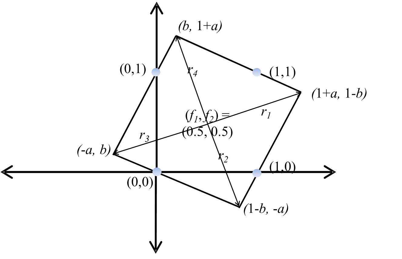
Figure 7: A general quadrilateral of our subclass.

Proof.

Let $Q$ be any maximal lattice-free quadrilateral in G. Q defines the valid inequality

$$\sum_{j=1}^{4}s_{j}\geq 1.$$ (19)

for $R_{f}(r_{1},\dots,r_{k})$. Let B be any maximal lattice-free triangle. Amongst the edges of B, atleast one edge has two of the points amongst (0,0), (0,1),(1,0) and (1,1) on one side and $f$ on the opposite side. Without loss of generality, this edge has (1,0) and (1,1) on one side and $f$ on the other side (Cornuéjols et al. [7]). This implies

$$\psi_{B}(r_{1})\geq\frac{0.5+a}{0.5}=\text{threshold}_{1}\hskip 4.0pt.$$ (20)

Treating $(r_{1},r_{4})$ as the basis, let $(\lambda_{1},\lambda_{2})$ be the co-ordinates of (1,1). Then it is easily checked that $(\lambda_{1},\lambda_{2})$ are also the co-ordinates of (1,0) with respect to the basis $(r_{2},r_{1})$, (0,0) with respect to the basis $(r_{3},r_{2})$ and (0,1) with respect to the basis $(r_{4},r_{3})$. It is also easily checked that

$$\lambda_{1}=\frac{0.5(1+a-b)}{(0.5+a)^{2}+(b-0.5)^{2}},\hskip 4.0pt\lambda_{2}=\frac{0.5(a+b)}{(0.5+a)^{2}+(b-0.5)^{2}}.$$ (21)

Let $f+r_{2}$ intersect $x_{1}=1$ at P (see Figure 8). Let the line joining P with origin intersect $f+r_{3}$ at $P^{\prime}$. It can be easily checked that the x co-ordinate of $P^{\prime}$ is given by

$$\frac{(a+b)(2b-1)}{(2b-1)^{2}+(2a+1)(a+b)}.$$ (22)

Let

$$\text{threshold}_{2}=\dfrac{0.5+a}{0.5-\dfrac{(a+b)(2b-1)}{((2b-1)^{2}+(2a+1)(a+b)}}.$$ (23)

Let

$$m=\frac{\lambda_{1}}{(2+(\lambda_{1}-\lambda_{2})(\text{threshold}_{1}+\text{threshold}_{2}))}.$$ (24)

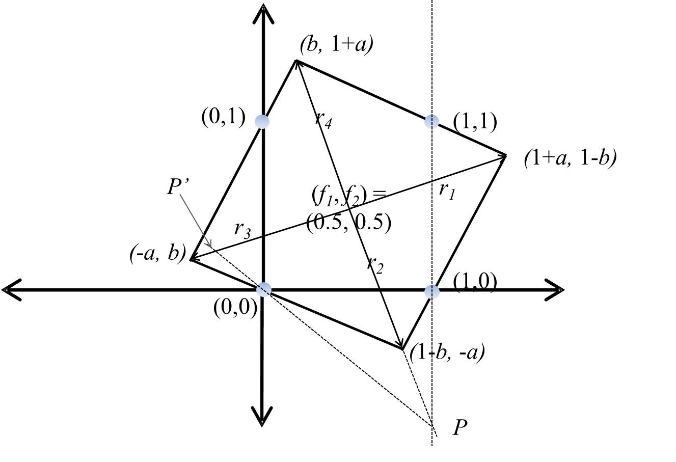
Figure 8: A construction which determines the cases for our proof.

Let the point $\bar{s}$ be defined as

$$\bar{s}=(m,m,m,m).$$ (25)

We now follow two cases for our analysis. Case 1 assumes $\psi_{B}(r_{3})\geq\text{threshold}_{2}$ and Case 2 assumes $\psi_{B}(r_{3})<\text{threshold}_{2}$.

Case 1: We note that (1,0) has to be above the line $\psi_{B}(r_{1})z_{1}+\psi_{B}(r_{2})z_{2}=1$, where $(z_{1},z_{2})$ denote the co-ordinates of (1,0) with respect to the basis $(r_{1},r_{2})$. This implies

$$\lambda_{2}\psi_{B}(r_{1})+\lambda_{1}\psi_{B}(r_{2})\geq 1.$$ (26)

Similarly,

$$\lambda_{2}\psi_{B}(r_{3})+\lambda_{1}\psi_{B}(r_{4})\geq 1.$$ (27)

From equations (26) and (27) and noting that $\lambda_{1}\geq\lambda_{2}$, we have

$$\lambda_{1}(\psi_{B}(r_{1})+\psi_{B}(r_{2})+\psi_{B}(r_{3})+\psi_{B}(r_{4}))\geq 2+(\lambda_{1}-\lambda_{2})(\psi_{B}(r_{1})+\psi_{B}(r_{3})).$$ (28)

Hence

$$\lambda_{1}(\psi_{B}(r_{1})+\psi_{B}(r_{2})+\psi_{B}(r_{3})+\psi_{B}(r_{4}))\geq 2+(\lambda_{1}-\lambda_{2})(\text{threshold}_{1}+\text{threshold}_{2}).$$ (29)

Hence

$$\frac{\lambda_{1}}{(2+(\lambda_{1}-\lambda_{2})(\text{threshold}_{1}+\text{threshold}_{2}))}(\psi_{B}(r_{1})+\psi_{B}(r_{2})+\psi_{B}(r_{3})+\psi_{B}(r_{4}))\geq 1.$$ (30)

From equation (30), $\bar{s}$ satisfies the minimal inequality defined by the maximal lattice-free triangle $B$. Hence $\bar{s}$ lies in the triangle closure. However, to satisfy the quadrilateral inequality $\sum_{j=1}^{4}s_{j}\geq 1$ defined by Q, we need to scale $\bar{s}$ by

$$q=\frac{(2+(\lambda_{1}-\lambda_{2})(\text{threshold}_{1}+\text{threshold}_{2})}{4\lambda_{1}}$$ (31)

$$=\big{(}(2\sqrt{(b(1-b))}+1)^{2}+(2b-1)^{2}\big{)}\frac{(\sqrt{(b(1-b))}-3b+2)}{4(\sqrt{b(1-b)}-b+1)^{2}}.$$ (32)

Case 2: As in Cornuéjols et al. [7], without loss of generality, we can assume that $w$ is a vertex of $B$ and that the line separating (1,0), (1,1) from $f$ is $x_{1}=1$. Hence,

$$\psi_{B}(r_{1})=\frac{0.5+a}{0.5}.$$ (33)

The maximality of B implies that each of (0,0) and (1,1) lies on a side of B. Hence

$$\lambda_{1}\psi_{B}(r^{3})+\lambda_{2}\psi_{B}(r^{2})=1.$$ (34)

$$\lambda_{1}\psi_{B}(r^{4})+\lambda_{2}\psi_{B}(r^{3})=1.$$ (35)

It can easily be checked that equations (33), (34), (35) imply equation (30). Hence, in this case as well, $\bar{s}$ lies in the triangle closure and needs to be scaled by $q$ in order to satisfy the quadrilateral inequality $\sum_{j=1}^{4}s_{j}\geq 1$ defined by Q.

From Cases 1 and 2, we obtain the bound $q$ given by equation (32). It is not difficult to confirm that the global maximum for this function of $b$ is 1.125 at $b=0.2$. This finishes the proof. ∎

The above result implies that for the structure $X$ defined by the intersection of the triangle closure and the set $S$ of minimal valid inequalities from maximal lattice-free quadrilaterals in the above subclass $G$, the approximation factor for approximation by the triangle closure is known to be exactly 1.125.

5 Conclusions

In this paper, for the two dimensional case, we improve on the state-of-the-art upper bound for the approximation of the Relaxed Corner Polyhedron (RCP) purely by the quadrilateral closure, from 2 to 1.71. We generalize the state-of-the-art lower bound of 1.125 for the approximation of the RCP purely by the triangle closure, to an infinite subclass of maximal lattice-free quadrilaterals.

6 Acknowledgements

The author would like to thank Gérard Cornuéjols for helpful discussions.

7 Appendix A.1

Here, we prove Lemma 18.

Proof.

$$x_{2}-0=-u(x_{1}-1)\text{ gives }\beta=-u(\alpha-1).$$ (36)

$$x_{2}=-vx_{1}\text{ gives }\beta=-v\alpha.$$ (37)

$$\text{Hence }\alpha(u-v)=u\text{ i.e. }\alpha=\frac{u}{u-v}\text{ i.e. }\alpha-1=\frac{v}{u-v}\text{ i.e. }\frac{1}{\alpha-1}=\frac{u-v}{v}=\frac{u}{v}-1.$$ (38)

$$x_{2}-1=w(x_{1}-0)\text{ gives }\delta-1=w\gamma.$$ (39)

$$x_{2}-0=-u(x_{1}-1)\text{ gives }\delta=-u(\gamma-1).$$ (40)

$$\text{ Hence }\gamma=\frac{\delta-1}{w}=-\frac{\delta}{u}+1\text{ i.e. }\delta=\frac{u(w+1)}{u+w}\text{ i.e. }\delta-1=\frac{w(u-1)}{u+w}\text{ i.e. }\frac{1}{\delta-1}=\frac{u+w}{w(u-1)}.$$ (41)

$$x_{1}=-vx_{1}\text{ gives }\zeta=v\epsilon.$$ (42)

$$x_{2}-1=w(x_{1}-0)\text{ gives }\zeta-1=-w\epsilon.$$ (43)

$$\text{ Hence }\zeta=v\epsilon=-w\epsilon+1\text{ i.e. }\epsilon=\frac{1}{v+w}\text{ and }\zeta=\frac{v}{v+w}.$$ (44)

$$\text{ The line passing through }(f_{1},f_{2})\text{, }(-\epsilon,\zeta)\text{ is }(\theta-f_{2})=\Bigg{(}\dfrac{f_{2}-\dfrac{v}{v+w}}{f_{1}+\dfrac{1}{v+w}}\Bigg{)}(-\theta-f_{1}).$$ (45)

$$\text{ Thus }\theta\Bigg{(}1+\dfrac{f_{2}-\dfrac{v}{v+w}}{f_{1}+\dfrac{1}{v+w}}\Bigg{)}=f_{2}-f_{1}\Bigg{(}\dfrac{f_{2}-\dfrac{v}{v+w}}{f_{1}+\dfrac{1}{v+w}}\Bigg{)}.$$ (46)

$$\text{ Thus }\theta\Bigg{(}\dfrac{f_{1}+\dfrac{1}{v+w}+f_{2}-\dfrac{v}{v+w}}{f_{1}+\dfrac{1}{v+w}}\Bigg{)}=\dfrac{f_{2}\Big{(}f_{1}+\dfrac{1}{v+w}\Big{)}-f_{1}\Big{(}f_{2}-\dfrac{v}{v+w}\Big{)}}{f_{1}+\dfrac{1}{v+w}}.$$ (47)

$$\text{ Thus }\theta\Bigg{(}\dfrac{(f_{1}+f_{2})(v+w)+(1-v)}{v+w}\Bigg{)}=\dfrac{f_{1}v+f_{2}}{v+w}.$$ (48)

$$\text{ Thus }\theta=\dfrac{f_{1}v+f_{2}}{(f_{1}+f_{2})(v+w)+(1-v)}.$$ (49)

$$\text{ Hence }\dfrac{\theta+f_{1}}{\epsilon-\theta}=\dfrac{\dfrac{f_{1}v+f_{2}}{(f_{1}+f_{2})(v+w)+(1-v)}+f_{1}}{\dfrac{1}{v+w}-\dfrac{f_{1}v+f_{2}}{(f_{1}+f_{2})(v+w)+(1-v)}}.$$ (50)

$$=\dfrac{(v+w)\Bigg{(}f_{1}v+f_{2}+f_{1}\Big{(}(f_{1}+f_{2})(v+w)+(1-v)\Big{)}\Bigg{)}}{(f_{1}+f_{2})(v+w)+(1-v)-(f_{1}v+f_{2})(v+w)}.$$ (51)

$$=\dfrac{(v+w)\Bigg{(}f_{2}\Big{(}1+f_{1}(v+w)\Big{)}+f_{1}^{2}(v+w)+f_{1}\Bigg{)}}{f_{1}(v+w)(1-v)+(1-v)}.$$ (52)

$$\text{ i.e. }\dfrac{\theta+f_{1}}{\epsilon-\theta}=\dfrac{(v+w)(f_{1}+f_{2})\Big{(}1+f_{1}(v+w)\Big{)}}{.}{(1-v)\Big{(}1+f_{1}(v+w)\Big{)}}.$$ (53)

$$\text{ Hence }\dfrac{\theta+f_{1}}{\epsilon-\theta}\text{=}\dfrac{(f_{1}+f_{2})(v+w)}{1-v}.$$ (54)

$$\text{ Thus }\dfrac{1-f_{1}}{\alpha-1}+\dfrac{1-f_{2}}{\delta-1}+\dfrac{\theta+f_{1}}{\epsilon-\theta}=(1-f_{1})(\frac{u}{v}-1)+(1-f_{2})\dfrac{u+w}{w(u-1)}+\dfrac{(f_{1}+f_{2})(v+w)}{1-v}.$$ (55)

∎

References

- [1] K. Andersen, Q. Louveaux, R. Weismantel, and L. A. Wolsey. Inequalities from two rows of a simplex tableau. In IPCO, pages 1–15, 2007.
- [2] A. Basu, P. Bonami, G. Cornuéjols, and F. Margot. On the relative strength of split, triangle and quadrilateral cuts. Math. Program., 126(2):281–314, 2011.
- [3] A. Basu, G. Cornuéjols, and M. Molinaro. A probabilistic analysis of the strength of the split and triangle closures. In IPCO, pages 27–38, 2011.
- [4] D. Bell. A theorem concerning the integer lattice. Studies in Applied Mathematics, 56:187–188, 1977.
- [5] V. Borozan and G. Cornuéjols. Minimal valid inequalities for integer constraints. Math. Oper. Res., pages 538–546, 2009.
- [6] G. Cornuéjols, M. Conforti, and G. Zambelli. Integer Programming. Unpublished, 1st edition, 2011.
- [7] G. Cornuéjols, B. Guenin, and L. Tuncel. Strength of triangle closure. Unpublished, 2010.
- [8] S. S. Dey and L. A. Wolsey. Lifting integer variables in minimal inequalities corresponding to lattice-free triangles. In IPCO, pages 463–475, 2008.
- [9] J. P. Doignon. Convexity in crystallographical lattices. Journal of Geometry, 3:71–85, 1973.
- [10] M. X. Goemans. Worst-case comparison of valid inequalities for the TSP. Math. Program., 69:335–349, 1995.
- [11] R. E. Gomory. Some polyhedra related to combinatorial problems. Linear Algebra and Its Applications, 2:451–558, 1969.
- [12] L. Lov´asz. Geometry of numbers and integer programming. Mathematical Programming: Recent Developments and Applications, M. Iri and K. Tanabe eds., Kluwer (1989), pages 177–210, 1989.
- [13] H. Scarf. An observation on the structure of production sets with indivisibility. In Proceedings of the National Academy of Sciences of the United States of America, volume 74, pages 3637–3641, 1977.