On the dissipative non-minimal braneworld inflation

Abstract

We study the effects of the non-minimal coupling on the dissipative dynamics of the warm inflation in a braneworld setup, where the inflaton field is non-minimally coupled to induced gravity on the warped DGP brane. A warped DGP scenario is a hybrid model containing both DGP and RSII character. We study with details the effects of the non-minimal coupling and dissipation on the inflationary dynamics on the normal DGP branch of this hybrid scenario in the high-dissipation and high-energy regime. We show that incorporation of the non-minimal coupling in this setup decreases the number of e-folds relative to the minimal case. We also compare our model parameters with recent observational data.

1 Introduction

Standard big bang cosmology, with its great successes in confrontation with observational data, has several shortcomings, part of which can be explained naturally in inflation paradigm. Inflation is also a successful scenario for production and evolution of the perturbations in primary stages of the universe evolution (Liddle & Lyth, 2000). While inflationary scenario is successful in these respects, there is a problem for realization of this scenario that we do not know how to integrate it with ideas of particle physics (Brandenberger, 2005; Lidsey et al., 1997). From a thermodynamic viewpoint, there are two dynamical realizations of inflation: In the standard inflation scenario known as supercooled inflation, radiation is red-shifted during expansion and a vacuum dominated universe is the result of this exponential expansion. This picture gives an isentropic perspective of the inflation paradigm. In this picture, the universe expands in inflation phase and its temperature decrease rapidly. When inflation ends, a reheating period introduces radiation into the universe. The fluctuations during this inflation phase are zero-point ground state fluctuations and evolution of the inflaton field is governed by the ground state evolution equation. In this model, there are no thermal perturbations and therefore, density perturbations are adiabatic. To have a radiation dominated universe at the end of this inflationary phase, a reheating period is needed to fill the universe with radiation. This model separates expansion and reheating into two distinguished time periods. However, energy transfer from potential energy to radiation is a nontrivial aspect of this supercooled inflation. As a second alternative, warm inflation proposed firstly by Berrera, is a successful scenario to overcome this difficulty (Berera, 1995; Berera & Kephart, 1999; Bellini, 1999a; Berera, 2000; Bellini, 1999b; Brandenberger & Ymaguchi, 2003; Hall et al., 2004a; Gupta, 2006; Hall et al., 2004b; Berera, 2005a; Bastero-Gil & Berera, 2007; Berera, 2006; Berera et al., 2009; Moss & Xiong, 2008; zhang, 2009; Romero & Bellini, 2009; del Campo et al., 2010; Matsuda, 2010; Bueno Sanches et al., 2011; Cai, 2011; Bastero-Gil et al., 2011). In this scenario, due to inflaton interactions with other fields, dissipative effects arise so that radiation production occurs concurrently with exponential expansion. Several mechanisms for implementing such a dissipation during inflation have been proposed (Berera & Kephart, 1999; Berera & Ramos, 2001; Dymnikova & Khlopov, 2004; Berera & Ramos, 2003, 2005b; Hall & Moss, 2005). For instance, a permanent or temporary coupling of the scalar field with other fields can lead to dissipative effects producing entropy at different eras of inflationary stage. In warm inflation proposal, matter and radiation energy fluctuations, which are responsible for temperature fluctuations, are treated separately. Matter fields interact with particles that are in a thermal bath with mean temperature smaller than grand unified theories (GUT) critical temperature (Bellini, 2001). Although this scenario is successful enough, it suffers from difficulties such as unjustified initial thermal bath which is needed to be introduced in the framework of chaotic inflation. One important feature of the inflationary paradigm is the fact that inflaton can interact with other fields such as gravitational sector of the theory. This interaction is shown by the non-minimal coupling of the inflaton field and Ricci scalar in the spirit of the scalar-tensor theories. In fact, there are several compelling reasons for inclusion of an explicit non-minimal coupling of the inflaton field and gravity in the action. For instance, non-minimal coupling arises at the quantum level when quantum corrections to the scalar field theory are considered. Even if for the classical, unperturbed theory this non-minimal coupling vanishes, it is necessary for the renormalizability of the scalar field theory in curved space. In most theories used to describe inflationary scenarios, it turns out that a non-vanishing value of the coupling constant cannot be avoided. Also, in general relativity, and in all other metric theories of gravity in which the scalar field is not part of the gravitational sector, the coupling constant necessarily assumes the value of   $\frac{1}{6}$  (Faraoni, 1996; Nozari, 2007a; Faraoni, 2000; Bouhamadi-Lopez & Wands, 2005; Nozari & Fazlpour, 2007b; Fakir & Unruh, 1990; Nozari & Fazlpour, 2008a; Uzan, 1990; Nozari & Shoukrani, 2009; Tsujikawa, 2000; Koh, 2005; Tsujikawa & Gumjudpai, 2004; Nozari & Sadatian, 2008b; Kofinas et al., 2003; Linde et al., 2011). Thus, it is natural to study an extension of the warm inflation proposal that contains explicit non-minimal coupling of the scalar field and gravity. We call this extension as non-minimal warm inflation. Although this issue has been considered by some authors, but there are very limited number of studies in this direction (Bellini, 2002). So, there is enough motivation to study warm inflation with non-minimally coupled inflaton field.

On the other hand, theories of extra spatial dimensions, in which the observed universe is realized as a brane embedded in a higher dimensional spacetime, have attracted a lot of attention in the last few years. In this framework, ordinary matters are trapped on the brane, but gravitation propagates through the entire spacetime (Arkani-Hamed et al., 1998; Antoniadis et al., 1998; Arkani-Hamed et al., 1999; Randall & Sundrum, 1999a, b; Dvali et al., 2000). The cosmological evolution on the brane is given by an effective Friedmann equation that incorporates the effects of the bulk in a non-trivial manner (Bin$\acute{e}$truy et al., 2000; Maartens & Koyama, 2010). Other extensions of the warm inflation proposal to braneworld scenario have been studied by some authors (Maeda et al., 2003; Antonella Cid et al., 2007).

With these preliminaries, the goal of the present study is to investigate a braneworld viewpoint of warm inflation with an explicit non-minimal coupling of the scalar field and Ricci curvature on the brane. We study possible impact of the non-minimal coupling and dissipation on the dynamics of these braneworld-inspired warm inflation. Our setup is based on warped DGP braneworld model in the platform constructed in (Maeda et al., 2003; Antonella Cid et al., 2007), but we incorporate an explicit nonminimal coupling of the scalar field and gravity on the brane. We study parameter space of each model in the high dissipation limit. As we will show, this model provides a natural exit from inflationary phase without adopting any additional mechanism. We show also that incorporation of the non-minimal coupling in this setup decreases the number of e-folds relative to the minimal case. Confrontation with combined WMAP7+BAO+$H_{0}$ dataset shows that this model in the high dissipation limit mostly gives a red and nearly scale invariant power spectrum.
Through this paper a dot on a quantity marks its time differentiation, while a prime denotes differentiation with respect to the scalar field, $\varphi$.

2 The Setup

We start with the following action to construct a braneworld non-minimal inflation scenario

$$S=\frac{1}{2\kappa_{5}^{2}}\int_{y\neq 0}d^{5}X\sqrt{-g^{(5)}}\big{(}R^{(5)}-2\Lambda_{5}\big{)}+\int_{y=0}d^{4}x\sqrt{-g}\bigg{[}\frac{R}{2\kappa_{4}^{2}}-\frac{1}{2}g^{\mu\nu}\partial_{\mu}\varphi\partial_{\nu}\varphi-\frac{1}{2}\xi R\varphi^{2}-V(\varphi)-\lambda\bigg{]}$$ (1)

In this action, which is written in the Jordan frame, $X$ is coordinate in the bulk, while $x$ shows induced coordinate on the brane.  $\kappa_{5}^{2}$ is the $5$-dimensional gravitational constant, $R^{(5)}$ is 5-dimensional Ricci scalar and $\xi$ is the nonminimal coupling (NMC) of the scalar field $\varphi$ and Ricci curvature on the brane,  $\Lambda_{4}=\frac{1}{2}(\Lambda_{5}+\kappa_{4}^{2}\lambda)$  is the effective cosmological constant on the brane,$\Lambda_{5}$ is the 5-dimensional cosmological constant in the bulk, so that $\Lambda_{4}=0$, at least in the early universe and $\lambda$ is the brane tension.

We have chosen a conformal coupling of the inflaton and gravity on the brane for simplicity. In other words, non-minimal coupling of the scalar field and gravity on the brane is $\alpha(\varphi)=\frac{1}{2}(1-\xi\varphi^{2})$ ( with $\kappa_{4}^{2}=8\pi G=1$). Variation of the action with respect to $\varphi$ leads to the equation of dynamics for scalar field on the brane

$$\ddot{\varphi}+3H\dot{\varphi}+\xi R\varphi+\frac{dV}{d\varphi}=0,$$ (2)

where $R=6(\frac{\ddot{a}}{a}+\frac{\dot{a}^{2}}{a^{2}})$  for spatially flat FRW geometry on the brane and $H=\frac{\dot{a}}{a}$ is the brane Hubble parameter. If we consider phenomenologically a dissipation coefficient $\Gamma$ that is responsible for the decay of the scalar field into radiation during the inflationary regime, equation of dynamics for the scalar field will be as follows

$$\ddot{\varphi}+3H\dot{\varphi}+\xi R\varphi+\frac{dV}{d\varphi}=-\Gamma\dot{\varphi}$$ (3)

$\Gamma$ can be assumed to be a constant or a function of the scalar field $\varphi$ or the temperature $T$, or both of them. We should emphasize that usually the dissipative coefficient is a function of the temperature of the thermal plasma because the dissipative effect arises from the relaxation process of the thermal plasma and vanishes at zero-temperature. For the case where the dissipative coefficient depends on the temperature of the thermal plasma, we refer to Ref.(Berera, 1995; Berera & Kephart, 1999; Bellini, 1999a; Berera, 2000; Bellini, 1999b; Brandenberger & Ymaguchi, 2003; Hall et al., 2004a; Gupta, 2006; Hall et al., 2004b; Berera, 2005a; Bastero-Gil & Berera, 2007; Berera, 2006; Berera et al., 2009; Moss & Xiong, 2008; zhang, 2009; Romero & Bellini, 2009; del Campo et al., 2010; Matsuda, 2010; Bueno Sanches et al., 2011; Cai, 2011; Bastero-Gil et al., 2011). In which follows for simplicity we assume that $\Gamma$ is only a function of $\varphi$ which itself is a function of the cosmic time. By the second Law of thermodynamics, $\Gamma$ must satisfies the condition $\Gamma=f(\varphi)>0$.

In the slow-roll approximation where $\ddot{\varphi}\ll|3H\dot{\varphi}|$, equation of motion for the scalar field takes the following form

$$\dot{\varphi}=-\frac{\xi R\varphi+V^{\prime}(\varphi)}{\Gamma+3H}.$$ (4)

The energy density and pressure of the non-minimally coupled scalar field are given by

$$\rho_{\varphi}=\frac{1}{2}\dot{\varphi}^{2}+V(\varphi)+6\xi H\varphi\dot{\varphi}+3\xi H^{2}\varphi^{2}$$ (5)

and

$$P_{\varphi}=\frac{1}{2}\dot{\varphi}^{2}-V(\varphi)-2\xi\varphi\ddot{\varphi}-2\xi\dot{\varphi}^{2}-4\xi H\varphi\dot{\varphi}-\xi(2\dot{H}+3H^{2})\varphi^{2}$$ (6)

respectively. The conservation equation for scalar field energy density in this setup is given by

$$\dot{\rho}_{\varphi}+3H(\rho_{\varphi}+P_{\varphi})=\dot{\varphi}V^{\prime}+\dot{\varphi}\ddot{\varphi}+3H\dot{\varphi}^{2}+\xi R\varphi\dot{\varphi}$$ (7)

where from equation (3) we find

$$\dot{\rho}_{\varphi}+3H(\rho_{\varphi}+P_{\varphi})=-\Gamma\dot{\varphi}^{2}$$ (8)

During inflaton evolution, dissipation leads to production of entropy. The entropy density of the radiation $S(\varphi,T)$ in this non-minimal setup is defined by $S=-\int(\frac{dV(\varphi)}{T})$. Now the total energy density of the system is defined by

$$\rho=\frac{1}{2}\dot{\varphi}^{2}+V(\varphi)+6\xi H\varphi\dot{\varphi}+3\xi H^{2}\varphi^{2}+TS$$ (9)

and using relation (8) the rate of entropy production can be deduced. In this non-minimal setup, entropy production is affected by the non-minimal coupling of gravity and inflaton field. This can be seen more explicitly in the following relation

$$T(\dot{S}+3HS)=\Gamma\dot{\varphi}^{2},$$ (10)

where by equation (4),  $\dot{\varphi}$ is directly related to the non-minimal coupling. The basic idea of warm inflation is that radiation production is occurring concurrently with inflationary expansion due to dissipation from the inflaton field system. The equation of state for radiation is given by $P_{\gamma}=\frac{\rho_{\gamma}}{3}$. Therefore, the conservation equation of $\rho_{\gamma}$ yields the following result

$$\dot{\rho}_{\gamma}+4H\rho_{\gamma}=\Gamma\dot{\varphi}^{2}.$$ (11)

It is interesting to note that time evolution of the radiation field is related to the non-minimal coupling via $\dot{\varphi}$. Following (Maeda et al., 2003; Antonella Cid et al., 2007), we assume a quasi-stable radiation production during the warm inflation phase, namely we assume that $\dot{\rho}_{\gamma}\ll 4H\rho_{\gamma}$ and $\dot{\rho}_{\gamma}\ll\Gamma\dot{\varphi}^{2}$, so we can write

$$\rho_{\gamma}\approx\frac{\Gamma}{4H}\dot{\varphi}^{2}.$$ (12)

In the slow-roll approximation, $\rho_{\varphi}$ and $\rho_{\gamma}$ attain the following approximate forms respectively

$$\rho_{\varphi}\approx V(\varphi)+6\xi H\varphi\dot{\varphi}+3\xi H^{2}\varphi^{2},$$ (13)

$$\rho_{\gamma}\approx 0.$$ (14)

we use these approximate forms in equation (17)to find cosmological dynamics of the model . We define the dissipation factor as follows

$$Q\equiv\frac{\Gamma}{3H},$$ (15)

which is a dimensionless parameter. With this definition, we can write

$$\dot{\varphi}=-\frac{\xi R\varphi+V^{\prime}(\varphi)}{3H(1+Q)}$$ (16)

During the slow-roll stage, the scalar field evolution is damped. For the high (or weak) dissipation regime we have $Q\gg 1$(or $Q\ll 1$) respectively. Now the Friedmann equation of the model takes the following form ( for details of calculations see the paper by Nozari and Fazlpour in (Faraoni, 1996; Nozari, 2007a; Faraoni, 2000; Bouhamadi-Lopez & Wands, 2005; Nozari & Fazlpour, 2007b; Fakir & Unruh, 1990; Nozari & Fazlpour, 2008a; Uzan, 1990; Nozari & Shoukrani, 2009; Tsujikawa, 2000; Koh, 2005; Tsujikawa & Gumjudpai, 2004; Nozari & Sadatian, 2008b; Kofinas et al., 2003; Linde et al., 2011) which considers a general non-minimal Gauss-Bonnet scenario with induced gravity. See also the paper by Kofinas et al. in (Faraoni, 1996; Nozari, 2007a; Faraoni, 2000; Bouhamadi-Lopez & Wands, 2005; Nozari & Fazlpour, 2007b; Fakir & Unruh, 1990; Nozari & Fazlpour, 2008a; Uzan, 1990; Nozari & Shoukrani, 2009; Tsujikawa, 2000; Koh, 2005; Tsujikawa & Gumjudpai, 2004; Nozari & Sadatian, 2008b; Kofinas et al., 2003; Linde et al., 2011))

$$H^{2}+\frac{k}{a^{2}}-\frac{{\cal{E}}_{0}}{a^{4}}=\Bigg{[}r_{c}\alpha(\varphi)\big{(}H^{2}+\frac{k}{a^{2}}\big{)}-\frac{\kappa_{5}^{2}}{6}\big{(}\rho+\lambda\big{)}\Bigg{]}^{2}$$ (17)

where we assume that the metric on the brane is spatially flat FRW type $(k=0)$.  $r_{c}=\frac{\kappa_{5}^{2}}{2\kappa_{4}^{2}}$ , is the induced-gravity crossover length scale, $\rho$ is the total energy density on the brane, namely $\rho=\rho_{\varphi}+\rho_{\gamma}$. Also ${\cal{E}}_{0}$ is a constant related to the 5-dimensional Weyl tensor describing the effect of the bulk graviton degrees of freedom on the brane dynamics and corresponding term is called dark radiation term. Note that the bulk cosmological constant appears implicitly via $\lambda$ that  $\Lambda_{4}=\frac{1}{2}(\Lambda_{5}+\kappa_{4}^{2}\lambda)$ .
Note that in (17) if we consider a flat brane $(k=0)$ with $\lambda=0$ and also a Minkowski bulk $(\Lambda_{5}=0,{\cal{E}}_{0}=0)$, then we recover the pure DGP solution as follows

$$H^{2}=\pm\frac{H}{r_{c}\alpha(\varphi)}+\frac{{\kappa_{4}^{2}}}{{3\alpha(\varphi)}}\rho.$$ (18)

In this work we consider the case with $\Lambda_{4}$.

$$H^{2}-\frac{{\cal{E}}_{0}}{a^{4}}=\Bigg{[}r_{c}\alpha(\varphi)H^{2}-\frac{\kappa_{5}^{2}}{6}\bigg{(}V(\varphi)-\frac{2\xi^{2}R\varphi^{2}+2\xi\varphi V^{\prime}}{1+Q}+3\xi H^{2}\varphi^{2}+\lambda\bigg{)}\Bigg{]}^{2}$$ (19)

Using the definition of $\dot{\varphi}$ as given by equation (16), this leads to a forth order equation for Hubble parameter of the model

$$H^{4}\Big{(}r_{c}\alpha(\varphi)-\frac{\xi\varphi^{2}\kappa_{5}^{2}}{2}\Big{)}^{2}-H^{2}\Bigg{[}1+2\Big{(}r_{c}\alpha(\varphi)-\frac{\xi\varphi^{2}\kappa_{5}^{2}}{2}\Big{)}\Bigg{(}\frac{\kappa_{5}^{2}}{6}\Big{(}V(\varphi)-\frac{2\xi^{2}R\varphi^{2}+2\xi\varphi V^{\prime}}{1+Q}+\lambda\Big{)}\Bigg{)}\Bigg{]}$$

$$+\Bigg{[}\frac{\kappa_{5}^{2}}{6}\Big{(}V(\varphi)-\frac{2\xi^{2}R\varphi^{2}+2\xi\varphi V^{\prime}}{1+Q}+\lambda\Big{)}\Bigg{]}^{2}+\frac{{\cal{E}}_{0}}{a^{4}}=0.$$ (20)

By assuming a non-vanishing non-minimal coupling, that is if $\xi\neq 0$, we can solve equation (20) for $H^{2}$ to find the following solutions

$$H^{2}=\frac{\lambda}{b^{2}}\,\Big{[}\,\frac{8\pi}{m_{p}^{2}}+\frac{8\pi r_{c}}{3m_{p}^{2}}\,b\,(1+\frac{d}{\lambda})\,\Big{]}\pm\frac{2}{b}\,\sqrt{\frac{1}{b^{2}}+\frac{r_{c}}{b}(1+\frac{d}{\lambda})-\frac{{4\cal{E}}_{0}}{a^{4}}}$$ (21)

where $d$ and $b$ are defined as follows

$$d\equiv V-\frac{2\xi\varphi}{1+Q}(\xi R\varphi+V^{\prime}),\quad\quad b\equiv r_{c}\alpha(\varphi)-\frac{3\xi\varphi^{2}\kappa_{5}^{2}}{2}.$$ (22)

Since we are interested in the inflationary dynamics of the model, we will neglect the dark radiation term in which follows.In this case, generalized Friedmann equation (21) attains the following form

$$H^{2}=\frac{\lambda}{b^{2}}\,\Big{[}\,\frac{8\pi}{m_{p}^{2}}+\frac{8\pi r_{c}}{3m_{p}^{2}}\,b\,(1+\frac{d}{\lambda})\,\Big{]}\pm\frac{2}{b}\,\sqrt{\frac{1}{b^{2}}+\frac{r_{c}}{b}(1+\frac{d}{\lambda})}$$ (23)

Note that the effective cosmological constant on the brane is determined by $\Lambda_{4}=\frac{4\pi}{m_{5}^{3}}\big{(}\Lambda_{5}+\frac{4\pi}{3m_{5}^{3}}\lambda^{2}\big{)}$ and the four-dimensional Plank scale is given by $m_{p}=\sqrt{\frac{3}{4\pi}}(\frac{m_{5}^{3}}{\sqrt{\lambda}})m_{5}$ . To be more specific, in which follows we consider just the minus sign in equation (23). Now, we define the slow-roll parameters as follows

$$\varepsilon\equiv-\frac{\dot{H}}{H^{2}},$$

$$\eta\equiv-\frac{\ddot{H}}{H\dot{H}}$$

and

$$\gamma^{2}\equiv 2\varepsilon\eta-\frac{d\eta}{dt}$$

We note that in the analysis of the warm inflation, the slow-roll conditions for thermal plasma should be considered too. In this respect we require that in equation (12) one should impose a condition for suppression of $\ddot{\rho_{\gamma}}$ (see for instance (Berera, 1995; Berera & Kephart, 1999; Bellini, 1999a; Berera, 2000; Bellini, 1999b; Brandenberger & Ymaguchi, 2003; Hall et al., 2004a; Gupta, 2006; Hall et al., 2004b; Berera, 2005a; Bastero-Gil & Berera, 2007; Berera, 2006; Berera et al., 2009; Moss & Xiong, 2008; zhang, 2009; Romero & Bellini, 2009; del Campo et al., 2010; Matsuda, 2010; Bueno Sanches et al., 2011; Cai, 2011; Bastero-Gil et al., 2011) for details). Since in our analysis we have not included the temperature dependence of the scalar field potential, the forth slow-roll parameter defined for thermal plasma is absent. We emphasize that the slow-roll approximation is valid when all of the slow-roll parameters are smaller than $1+Q$.

We need to calculate these parameters in our non-minimal dissipative braneworld model. For $\varepsilon$ we find

$$\varepsilon\approx\frac{2\dot{A}B-2\dot{B}A-\dot{C}C^{-1}A}{4H^{3}A},$$ (24)

where

$$A\equiv\frac{\Big{(}r_{c}\alpha(\varphi)-\frac{3\xi\varphi^{2}\kappa_{5}^{2}}{2}\Big{)}^{2}}{\lambda}$$

$$B\equiv\frac{8\pi}{m_{p}^{2}}+\frac{8\pi r_{c}}{3m_{p}^{2}}\,b\,(1+\frac{d}{\lambda}),$$

$$C\equiv\frac{4}{b^{4}}+\frac{4r_{c}}{b^{3}}\,(1+\frac{d}{\lambda})$$

and $d$ and $b$ are defined in equation (22). The second slow-roll parameter, $\eta$, is calculated as follows

$$\eta\approx\bigg{[}4A^{2}H^{3}(2\dot{B}A-2\dot{B}\dot{A}+\dot{C}C^{-1}A)\bigg{]}^{-1}\bigg{[}(8\dot{A}AH^{2}+2\dot{B}A-2\dot{A}B+\dot{C}C^{-1}A)(2\dot{B}A-2\dot{A}B+\dot{C}C^{-1}A)$$

$$-(2\ddot{B}A-2\ddot{A}B+\ddot{C}C^{-1}A-\dot{C}^{2}C^{-2}A+\dot{C}C^{-1}\dot{A})4A^{2}H^{2}\bigg{]}.$$ (25)

And finally, the third slow-roll parameter, $\gamma^{2}$, in our model takes the following form

$$\gamma^{2}\approx-\frac{\dot{\varphi}}{(1+Q)H}\bigg{(}\frac{V^{\prime\prime\prime}}{3H^{2}}-\frac{Q^{\prime}(V^{\prime\prime}+\xi R)}{3H^{2}(1+Q)}+Q^{\prime}\varepsilon\bigg{)}$$

$$-\frac{\dot{\varphi}^{2}}{(1+Q)H^{2}}\Big{(}Q^{\prime\prime}-\frac{Q^{\prime 2}}{1+Q}\Big{)}-\frac{Q^{\prime}(\xi R\varphi+V^{\prime})}{3(1+Q)^{2}H^{2}}\Big{(}\eta+\varepsilon-\frac{2Q^{\prime}\dot{\varphi}}{(1+Q)H}\Big{)}.$$ (26)

After constructing the basic formalism, we study inflationary dynamics of this non-minimal dissipative model. For this goal, in which follows and in all of our numerical calculations, we consider the well-known large-field inflationary potential $V(\varphi)=V_{0}\varphi^{n}$ to investigate outcomes of our model. The inflationary phase terminates if the condition $\varepsilon=1+Q$ is satisfied and this happens when radiation and potential energies satisfy an especial condition will be derived later on ( see equation (31)). Figure $1$ shows the variation of $\varepsilon$ versus the inflaton field in large field limit with $V(\phi)=V_{0}\varphi^{2}$. In this figure we have assumed high-dissipation and high energy limit with $Q\gg 1$ and $V\gg\lambda$ respectively. As this figure shows, this model has the capacity to accounts for natural exit from inflationary phase without any additional mechanism. In fact, non-minimal coupling of the inflaton field and gravity on the brane provides a suitable parameter space for natural exit of the inflationary phase. We stress that in this figure the minimal case with $\xi=0$ accounts for natural exit without additional mechanism too. This is possible in our setup because of the braneworld effect. We note that most inflationary models exit inflation naturally, e.g. chaotic, natural new inflation etc. But there are scenarios such as hybrid inflation that introduce a phase transition to terminate inflation. Figure $2$  shows the possibility of the natural exit from inflationary phase in high-dissipation ($Q\gg 1$) and high-energy limit ($V\gg\lambda$) for $V(\phi)=V_{0}\exp{\big{(}-\sqrt{\frac{2}{p}}\frac{\varphi}{m_{p}}}\big{)}$. We see that in this case incorporation of the non-minimal coupling and braneworld effects are sufficient for natural exit from inflationary phase too and there is no need to introduce additional mechanism to achieve this goal. Now the energy density of the radiation field as a function of the scalar field potential can be written as follows

$$\rho_{\gamma}=\frac{3Q}{4}\bigg{(}\frac{\xi R\varphi+V^{\prime}}{3(1+Q)}\bigg{)}^{2}\frac{\varepsilon}{\zeta},$$ (27)

where $\zeta\equiv\varepsilon H^{2}$. Since $\rho_{\gamma}=\sigma{T_{\gamma}}^{4}$, where $\sigma$ is the Stefan-Boltzmann constant and $T_{\gamma}$ is the temperature of the thermal bath, we find

$$T_{\gamma}=\Bigg{[}\frac{3Q}{4\sigma}\bigg{(}\frac{\xi R\varphi+V^{\prime}}{3(1+Q)}\bigg{)}^{2}\frac{\varepsilon}{\zeta}\Bigg{]}^{1/4}.$$ (28)

On the other hand, the relation between $\rho_{\gamma}$ and $\rho_{\varphi}$ is given by

$$\rho_{\gamma}=\bigg{[}\frac{3Q}{4}\Big{(}\frac{\xi R\varphi+V^{\prime}}{3(1+Q)}\Big{)}\frac{\varepsilon}{\zeta}\bigg{]}\bigg{(}\frac{V-\rho_{\varphi}+3\xi H^{2}\varphi^{2}}{2\xi\varphi}\bigg{)}.$$ (29)

Inflation occurs when the condition $\varepsilon<1+Q$ (or $\ddot{a}>0)$ is fulfilled. Therefore, using (28) we find

$$\rho_{\varphi}<-\bigg{(}\frac{2\xi\varphi}{\frac{Q}{4\zeta}(\frac{\xi R\varphi+V^{\prime}}{3(1+Q)})}\bigg{)}\rho_{\gamma}+V+3\xi H^{2}\varphi^{2},$$ (30)

which is the condition for realization of the non-minimal warm inflation on the brane. Note that $\zeta$ is a function of the 3-brane tension $\lambda$, and inflaton potential, $V$. Therefore, to have a warm inflationary period on the brane, the condition (30) should be fulfilled. As we have pointed out previously, inflationary phase will terminates when the universe heats up so that the condition $\varepsilon=1+Q$ is satisfied. In our non-minimal case this implies that

$$\rho_{\varphi}\simeq-\bigg{(}\frac{2\xi\varphi}{\frac{Q}{4\zeta}(\frac{\xi R\varphi+V^{\prime}}{3(1+Q)})}\bigg{)}\rho_{\gamma}+V+3\xi\zeta\varphi^{2}.$$ (31)

By comparison with the minimal case as has been studied in Ref. (Maeda et al., 2003; Antonella Cid et al., 2007), we see that non-minimal coupling of the scalar field and gravity on the brane has important role on the natural exit of the inflationary phase. This role has been highlighted in figures $1$ and $2$.

Now we focus on the number of e-foldings as another important quantity in a typical inflation scenrio. The number of e-foldings is defined as

$$N\equiv\int_{t_{i}}^{t_{end}}Hdt=\int_{\varphi_{i}}^{\varphi_{end}}\frac{H}{\dot{\varphi}}d\varphi$$

In our setup, the number of e-foldings at the end of the inflation phase is given by

$$N=-\int_{\varphi_{i}}^{\varphi_{e}}\bigg{(}\frac{3H^{2}(1+Q)}{\xi R\varphi+V^{\prime}}\bigg{)}d\varphi.$$ (32)

Using the explicit form of $H^{2}$ with negative sign as given by equation (23), the number of e-foldings in our non-minimal setup takes the following form

$$N=-\int_{\varphi_{i}}^{\varphi_{e}}\bigg{(}\frac{3(1+Q)}{\xi R\varphi+V^{\prime}}\bigg{)}\Bigg{\{}\frac{\lambda}{b^{2}}\Big{[}\frac{8\pi}{m_{p}^{2}}+\frac{8\pi r_{c}}{3m_{p}^{2}}\,b\,(1+\frac{d}{\lambda})\Big{]}-\frac{2}{b}\,\sqrt{\frac{1}{b^{2}}+\frac{r_{c}}{b}(1+\frac{d}{\lambda})}\Bigg{\}}d\varphi$$ (33)

with $d$ and $b$ as defined in (22).  $\varphi_{i}$ denotes the value of the scalar field $\varphi$ when universe scale observed today crosses the Hubble horizon during inflation, while $\varphi_{e}$ is the value of the scalar field when the universe exists the inflationary phase. The role played by the dissipation factor is the same as the minimal case studied in (Maeda et al., 2003; Antonella Cid et al., 2007): in the high-energy and high-dissipation limit where $V\gg\lambda$ and $Q\gg 1$ respectively, the rate of expansion is increased in comparison with the case in standard inflationary model, while in the low energy limit and weak dissipation where $V\ll\lambda$ and $Q\ll 1$ respectively, the rate of expansion is nearly the same as standard inflationary model. In our non-minimal case, the role played by the non-minimal coupling is not so trivial due to complicated form of the equation (33). To treat this problem, we define

$$g\equiv-\bigg{(}\frac{3(1+Q)}{\xi R\varphi+V^{\prime}}\bigg{)}\Bigg{\{}\frac{\lambda}{b^{2}}\Big{[}\frac{8\pi}{m_{p}^{2}}+\frac{8\pi r_{c}}{3m_{p}^{2}}\,b\,(1+\frac{d}{\lambda})\Big{]}-\frac{2}{b}\,\sqrt{\frac{1}{b^{2}}+\frac{r_{c}}{b}(1+\frac{d}{\lambda})}\Bigg{\}}$$

The number of e-foldings is the area enclosed between $g$-curve and the horizontal axis from $\varphi_{i}$ to $\varphi_{e}$ in the $g-\varphi$ plane. Figure $3$ shows the variation of $g$ versus $\varphi$ for different values of the non-minimal coupling for $\Gamma=\Gamma_{0}\varphi^{2}$. In the high and low energy limits, the number of e-folds decreases by increasing the values of $\xi$ ( in the case that all other quantities are fixed). Therefore, incorporation of the non-minimal coupling in this setup essentially decreases the number of e-folds. In an approximate manner, if we assume that $\xi$ is a small parameter ( see for instance (Nozari & Sadatian, 2008c; Nozari & shafizadeh, 2010) to see viability of this assumption), in the low-energy ($V\ll\lambda$) and low-dissipation limit ($Q\ll 1$) we can ignore terms containing $\frac{d}{\lambda}$ in the equation defining the number of e-folds and the remaining expression leads to the result that number of e-foldings decreases by inclusion of the non-minimal coupling. We stress that this decreasing depends on the values of the non-minimal coupling, inflation potential and also the detailed form of the dissipative coefficient. In the high energy and high dissipation limit with $V\gg\lambda$ and $Q\gg 1$ respectively, the number of e-folds decreases by inclusion of the non-minimal coupling too. Now,we study scalar and tensor perturbations in this non-minimal dissipative model. In the case of scalar perturbations, the scalar and the radiation fields are interacting. These perturbations are supposed to be adiabatic on the brane. Dissipative effects can produce a variety of spectral index, ranging between red and blue, and thus producing the running blue to red spectral index suggested by WMAP data (Komatsu, 2008; Spergel, 2007; Jarosik et al., 2010).We note that in the background spacetime $\frac{{\cal{E}}_{0}}{a^{4}}=0$, and we can use equation (23) as Friedmann equation in this setup. But the perturbed FRW brane has a nonzero $\frac{{\cal{E}}_{0}}{a^{4}}$, which encodes the effects of the bulk gravitational field on the brane (Koyama & Maartens, 2006) and we have use the Friedmann equation (21). We define the scalar curvature perturbation amplitude of a given mode when re-enters the Hubble radius as follows

$$\delta_{H}=\frac{2}{5}\frac{H}{\dot{\varphi}}\delta\varphi.$$ (34)

We note that this expression is actually for 4-dimensional case; but as Maartens et al. have shown in Ref. (Maartens et al., 2000), it can be used in this braneworld setup too. Note that although we have used the usual spectrum for the field perturbations in this warm inflation scenario, but the presence of the non-minimal coupling is implicit in the form of Hubble parameter, $H$, in this setup. Given that this spectrum have been derived in a complete different set-up, to begin with without coupling of the scalar field to the Ricci scalar, it may hold in the scenario studied in this work if we use the form of $H$ dependent on the non-minimal coupling.

The scalar spectrum index is defined as follows

$$n_{s}=1+\frac{d\ ln\delta_{H}^{2}}{d\ lnk}$$ (35)

The interval in wave number is related to the number of e-foldings by the relation $d\ln k(\varphi)=-dN(\varphi)$. Substituting (16) into the relation (34) for $\delta_{H}$, we find ( we refer to the Ref. (Nozari et al., 2011) for detailed form of fluctuations in the warm inflation scenarios)

$$\delta_{H}^{2}=\frac{36}{25}\frac{H^{4}(1+Q)^{2}}{(\xi R\varphi+V^{\prime})^{2}}\delta\varphi^{2}$$ (36)

Using the slow-roll parameters, we have

$$n_{s}=1-\frac{7}{2}\varepsilon+\frac{3}{2}\eta-\frac{9Q^{\prime}\dot{\varphi}^{2}}{4(\xi R\varphi+V^{\prime})}$$ (37)

The running of the spectral index which is defined as

$$\alpha_{s}=\frac{dn_{s}}{d\ln k}$$ (38)

in our model takes the following form

$$\alpha_{s}=\frac{9}{2}(2\varepsilon\eta-4\varepsilon^{2})+\frac{3}{2}\Big{(}2\varepsilon\eta-\gamma^{2}\Big{)}-\frac{(\xi R\varphi+V^{\prime})}{12(1+Q)^{3}H^{4}}\bigg{[}Q^{\prime\prime}(\xi R\varphi+V^{\prime})+Q^{\prime}(\xi R+V^{\prime\prime})\bigg{]}$$

$$+\frac{Q^{\prime}(\xi R\varphi+V^{\prime})}{2(1+Q)^{3}H^{2}}\bigg{(}\frac{Q^{\prime}(\xi R\varphi+V^{\prime})}{3H^{2}(1+Q)}-(1+Q)\varepsilon\bigg{)}.$$ (39)

Now we study these quantities numerically to investigate implications of this non-minimal dissipative setup. Figure $4$ shows the variation of $n_{s}$ versus the inflaton field for different values of the non-minimal coupling in high-dissipation limit for $V=V_{0}\varphi^{2}$. Since $n_{s}\leq 1$, our non-minimal dissipative model favors a red power spectrum. Therefore, our model for this type of potential gives also a nearly scale invariant spectrum. The result of WMAP7 for $\Lambda$CDM gives $n_{s}=0.963^{+0.014}_{-0.014}$  for index of the power spectrum (Komatsu, 2008; Spergel, 2007; Jarosik et al., 2010). Combining WMAP7 with other data sources ( the Baryon Acoustic Oscillations (BAO) and$H_{0}$), gives $n_{s}=0.963^{+0.012}_{-0.012}$ (Komatsu, 2008; Spergel, 2007; Jarosik et al., 2010). These results show that a red power spectrum is favored and $n_{s}>1$ is disfavored even when gravitational waves are included, which constrains the models of inflation that can produce significant gravitational waves, such as chaotic or power-law inflation models, or a blue spectrum, such as hybrid inflation models. So, our model at least qualitatively is in agreement with recent observational data. If there is running of the spectral index, the constraints on the spectral index and its running are given by $n_{s}=1.017^{+0.042}_{-0.043}$   and $\frac{dn_{s}}{d\ln k}=-0.022^{+0.020}_{-0.020}$ respectively (Komatsu, 2008; Spergel, 2007; Jarosik et al., 2010). The special case with $n_{s}=1$ and $\frac{dn_{s}}{dl\ln k}=0$ results in the scale invariant spectrum. The significance of $n_{s}$ and $\frac{dn_{s}}{dl\ln k}$ is that different inflation models motivated by different physics make specific, testable predictions for the values of these quantities. In summary, we see that our dissipative non-minimal model mostly excludes blue spectrum in agreement with recent observational data. Figure $5$ shows the running of the spectral index versus the inflaton field in high-dissipation limit for $V=V_{0}\varphi^{2}$. As we see, there is no signature of a positive running of the spectral index in this setup with positive values of the non-minimal coupling. Note that a negative $\xi$ is theoretically interesting but it requires anti-gravitation and therefore has been excluded in our analysis. Now we pay attention to the tensorial perturbations. As it has been mentioned in Ref.(Bhattacharya et al., 2006), the generation of the tensor perturbations during inflation produces stimulated emission in the thermal background of gravitational waves. This process changes the tensor modes by an extra temperature dependent factor given by $\coth(\frac{k}{2T})$  where $T$ is the temperature of the thermal bath. The corresponding spectrum becomes

$$A_{g}^{2}=\frac{16\pi}{\mu^{2}}(\frac{H}{2\pi})^{2}\coth[\frac{k}{2T}],$$ (40)

where $H$ is given by equation (21) with negative sign. Note that we incorporated the bulk effects in this relation via the Hubble parameter of model which contains especially the effect of bulk radiation term. Using equation (36) and (40), in the limit of $Q\gg 1$ the tensor to scalar ratio is given by

$$r=\bigg{(}\frac{A_{g}^{2}}{P_{R}}\bigg{)}_{k=k_{i}}\simeq\frac{8\varphi}{9\sqrt{3}\mu^{2}}\Bigg{[}\frac{(\xi R\varphi+V^{\prime}(\varphi))}{TH^{3}Q^{5/2}}\coth(\frac{k}{2T})\Bigg{]}_{k=k_{i}}.$$ (41)

Here, $P_{R}=\frac{25}{4}\delta_{H}^{2}$ and $k_{i}$ is referred to $k=Ha$, the value of $k$ when the universe scale crosses the Hubble horizon during inflation. Our model with $V_{0}=1$,  $m_{p}=10^{19}$ GeV,  $Q=10^{4}$ and $T=2.4\times 10^{17}$ GeV gives $r<0.24$ which is comparable with the observationally supported value of $r<0.22$ from WMAP7+BAO+$H_{0}$ combined dataset. We note that the above choices of parameters to calculate scalar-to-tensor ratio, generate suitable amplitude of scalar perturbation well in the range of observationally supported value of $P_{R}\sim 5\times 10^{-5}$.

Finally, a point should be stressed about the issue of frames in our setup. There is a conformal transformation which transforms the action (1) ( which is written in the Jordan frame) to corresponding action in the Einstein frame. In the Einstein frame, the gravitational sector is expressed in terms of a re-scaled scalar field which is minimally coupled and evolves in a re-scaled potential, thereby simplifying the formalism. However, one has to keep in mind that the matter sector is strongly affected by such a conformal transformation since all of the matter fields are now non-minimally coupled to the re-scaled metric: in particular, stress tensor conservation in the matter sector is no longer ensured (Schimd et al., 2005). On the other hand, as Makino and Sasaki (Makino & Sasaki, 1991) and Fakir et al (Fakir et al., 1992) have shown, the amplitude of scalar perturbation in the Jordan frame exactly coincides with that in the Einstein frame. This proof (for details see (Komatsu & Futamase, 1999)) allows us to calculate the scalar power spectrum in the Jordan and Einstein frame. As a result, the scalar power spectrum has no dependence on the choice of frames, i.e., it is conformally invariant. So, our results can be compared to observations directly without any ambiguities (Komatsu & Futamase, 1999). This is an important point since one has to check validity of non-gravity experiments in Einstein frame. For instance, validity of electro-magnetic related experiments such as CMB experiment should be checked in Einstein frame. As Komatsu and Futamase have shown, the scalar power spectrum is independent on the choice of frames (Komatsu & Futamase, 1999). We terminate this section by pointing that from a statistical mechanics viewpoint, the interaction between quantum fields and a thermal bath in this warm inflation scenario could be illustrated by a general fluctuation-dissipation relation ( see for instance (Weiss, 1993)). Warm inflation was criticized on the basis that the inflaton cannot decay during the slow-roll phase (Yokoyama & Linde, 1999). However, in recent years, it has been shown that the inflaton can indeed decay during the slow-roll phase and now this scenario rests on solid theoretical grounds ( see for instance (Berera, 1995; Berera & Kephart, 1999; Bellini, 1999a; Berera, 2000; Bellini, 1999b; Brandenberger & Ymaguchi, 2003; Hall et al., 2004a; Gupta, 2006; Hall et al., 2004b; Berera, 2005a; Bastero-Gil & Berera, 2007; Berera, 2006; Berera et al., 2009; Moss & Xiong, 2008; zhang, 2009; Romero & Bellini, 2009; del Campo et al., 2010; Matsuda, 2010; Bueno Sanches et al., 2011; Cai, 2011; Bastero-Gil et al., 2011) and (Maeda et al., 2003; Antonella Cid et al., 2007)).

3 Summary

It is well-known that early universe was filled by radiation energy $(\rho_{\gamma})$ and vacuum energy $(\rho_{v})$ (with equation of state as $\rho_{v}=-p_{v}$). In the inflationary regime, with positively accelerated expansion, $\ddot{a}>0$, one has $\rho_{v}>\rho_{\gamma}$. At the end of the inflationary phase however, universe is radiation dominated and therefore inflation sustains vacuum energy density along expansion of scale factor and at the time of the end of inflation universe enters to the radiation dominated era. This mean that after the end of inflation the universe is radiation dominated but the inflaton field retains some of its potential energy, because the inflaton condensate does not need to decay to reheat inflation. In inflationary paradigm, inflaton can interact with other fields such as Ricci curvature. This interaction is shown by the non-minimal coupling (NMC) of the inflaton and gravity in the action of the scenario. There are many compelling reasons to include an explicit non-minimal coupling in the action. So, naturally we should include non-minimal coupling of gravity and inflaton in the action of the inflation scenario. Usually, by incorporation of the non-minimal coupling it is harder to realize inflation even with potential that are known to be inflationary in the minimal case. However, inclusion of the non-minimal coupling is inevitable from field theoretical viewpoint especially their renormalizability. From a thermodynamical viewpoint to the inflationary expansion, there are two dynamical realizations of inflation. Standard picture is isentropic inflation which is referred to as supercooled inflation. In this picture, universe expands in inflation phase and its temperature decrease rapidly. When inflation ends, a reheating period introduces radiation into the universe. The fluctuations in this type of inflation model are zero-point ground state fluctuations and evolution of the inflaton field is governed by a ground state evolution equations. In this type of models we have not any thermal perturbations and therefore, density perturbations are adiabatic. The other picture is a non-isentropic inflation or warm inflation. Warm inflation is a model of inflationary dynamics which by adopting it, we can release from reheating period. In warm inflation scenario, interaction between the inflaton and other fields causes the radiation energy density. In this picture, inflation terminates smoothly and radiation regime is dominated, without a reheating period. The fluctuations during inflation emerge from some excited states and the evolution of the inflaton has dissipative terms arising from the interaction of the inflaton with other fields. In this picture, dissipative effects are important during the inflation period. In warm inflation, density fluctuations arise from thermal fluctuations and this fluctuations in the radiation cause the entropy perturbations. This entropy fluctuations disappear before inflation ends. For this reason, solution of the warm inflation violates the adiabatic condition. In this model, inflaton interacts with a thermal bath in warm inflation period by a friction term and this causes decay of inflaton. The friction term itself enters into the dynamics of the scalar field equation as an ad hoc term. In fact, warm inflation predicts that inflaton interactions with surrounding fields during the inflationary period will result in a friction term in the equations of motion. In this scenario, the anisotropies seen in the CMB are produced by thermal fluctuations. As a promising feature, it may be possible to distinguish between warm inflation and standard supercooled inflation models using forthcoming satellite data. In this paper we have studied warm inflation by incorporating an explicit non-minimal coupling of the inflaton field and gravity on the normal branch of a warped DGP brane.We have studied also parameter space of the model in high dissipation and high energy limits. As we have shown, this model provides natural exit from the inflationary phase without adopting any additional mechanism(s) for appropriate values of the non-minimal coupling. By a numerical analysis in this case, we have shown that incorporation of the non-minimal coupling in this setup decreases the number of e-folds relative to the minimal case. We emphasize however that this result is sensitive to the details of the model parameters such the dissipation function, scalar field potential and the non-minimal coupling. A qualitative confrontation with WMAP7+BAO+$H_{0}$ combined data shows that this model in high dissipation limit gives a red and nearly scale invariant power spectrum for positive values of the non-minimal coupling. From another viewpoint, comparison of this non-minimal warm inflation model with observational data could provide more accurate constraints on the values of the non-minimal coupling. Since we have calculated the first order contributions in slow-roll parameters, our results are valid in both Jordan and Einstein frame. However, higher order corrections could lead to different results in these two frames.

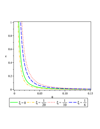
Figure 1: Variation of the $\varepsilon$ versus scalar field with $V(\phi)=V_{0}\varphi^{2}$ for different values of the non-minimal coupling in high-dissipation ($Q\gg 1$) and high-energy ($V\gg\lambda$) limit. There is the possibility to account for the condition $\varepsilon=1+Q$ which shows the end of the inflationary phase. This can be achieved naturally without any additional mechanism.

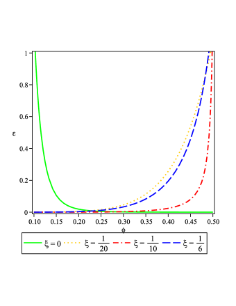
Figure 2: Variation of $\varepsilon$ versus $\varphi$ for different values of the non-minimal coupling in high-dissipation ($Q\gg 1$) and high-energy ($V\gg\lambda$) limit for $V(\phi)=V_{0}\exp{\big{(}-\sqrt{\frac{2}{p}}\frac{\varphi}{m_{p}}}\big{)}$ with $p=50$ and $m_{p}=1$. The condition $\varepsilon=1+Q$ which shows the end of the inflationary phase is achievable naturally in this setup without any additional mechanism.

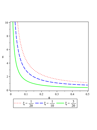
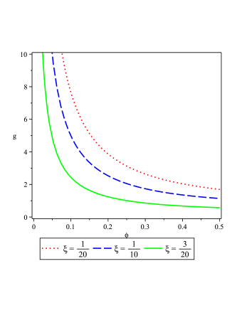
Figure 3: $g$ versus $\varphi$ in the limit of high ( left hand side) and low energy (right hand side) limits of the scenario with various values of the non-minimal coupling. Number of e-folds is given by the area bounded between $g$-curve and the horizontal axis in this $g-\varphi$ plot. In the high energy and low energy limits, the number of e-folds decreases by increasing the values of $\xi$. Therefore, incorporation of the non-minimal coupling in this setup essentially decreases the number of e-folds. Nevertheless, we stress that this decreasing depends on the values of the non-minimal coupling, inflation potential and also the detailed form of the dissipative coefficient.

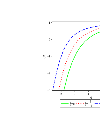
Figure 4: Variation of the spectral index $n_{s}$ versus inflaton field for different values of the non-minimal coupling in high-dissipation limit for $V=V_{0}\varphi^{2}$. Evidently, $n_{s}\leq 1$ and therefore our non-minimal model favors a red power spectrum and this is confirmed by recent observational data sets.

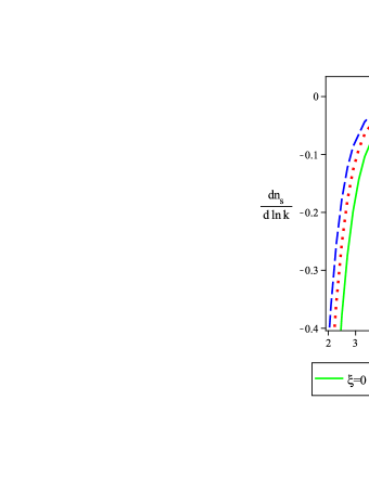
Figure 5: Running of the spectral index versus $\varphi$ in high-dissipation limit for potential $V=V_{0}\varphi^{2}$.

References

- Liddle & Lyth (2000) Liddle, A., Lyth, D., Cosmological Inflation and Large-Scale Structure, 2000, Cambridge University Press
- Brandenberger (2005) Brandenberger, R. H., 2005,[arXiv:hep-th/0509099]
- Lidsey et al. (1997) Lidsey, J. E. et al., 1997, Rev. Mod. Phys, 69, 373
- Berera (1995) Berera, A., 1995, Phys. Rev. Lett., 75, 3218
- Berera et al. (1999) Berera, A., Gleiser, M., & Ramos,R. O., 1999, Phys. Rev. Lett., 83,264
- Bellini (1999a) Bellini, M., 1999a, Class. Quant. Grav, 16, 2393
- Berera (2000) Berera, A., 2000, Nucl. Phys. B, 585,666
- Bellini (1999b) Bellini, M.,1999b, Nucl. Phys. B, 563, 245
- Brandenberger & Ymaguchi (2003) Brandenberger, R. H., & Ymaguchi,M., 2003, Phys. Rev. D, 68, 023505
- Hall et al. (2004a) Hall, L. M. H., Moss, I. G., & Berera, A., 2004a, Phys. Rev. D, 69, 083525
- Gupta (2006) Gupta, S., 2006, Phys. Rev. D, 73, 083514
- Hall et al. (2004b) Hall, L. M. H., Moss, I. G., & Berera, A., 2004b, Phys. Lett. B, 589, 1
- Berera (2005a) Berera, A., 2005a, Grav. Cosmol, 11, 51
- Bastero-Gil & Berera (2007) Bastero-Gil, M., & Berera, A., 2007, Phys. Rev. D, 76, 043515
- Berera (2006) Berera, A., 2006, Contemporary Physics, 47, 33
- Berera et al. (2009) Berera, A., Moss, I. G., & Ramos, R. O., 2009, Rept. Prog. Phys, 72, 026901
- Moss & Xiong (2008) Moss, I. G., & Xiong, C., 2008, J. Cosmology Astropart. Phys, 0811, 023
- zhang (2009) Zhang, Y., 2009, J. Cosmology Astropart. Phys, 0903, 023
- Romero & Bellini (2009) Romero, J. M., & Bellini, M., 2009 Nuovo Cim. B, 124, 861
- del Campo et al. (2010) del Campo, S., Herrera, R., Pavon,D., Pavon, & Villanueva, J.R., 2010,[arXiv:1007.0103]
- Matsuda (2010) Matsuda, T., 2010, J. Cosmology Astropart. Phys, 1011, 036
- Bueno Sanches et al. (2011) Bueno Sanches,J. C., Bastero-Gil, M., Berera, A., Dimopoulos, K., & Kohri, K., 2011, J. Cosmology Astropart. Phys, 1103, 020
- Cai (2011) Cai, Y. -F., Dent, J. B., & Easson, D. A., 2011, Phys. Rev. D, 83, 101301
- Bastero-Gil et al. (2011) Bastero-Gil, M., Berera, A.,& Rosa, J. G., 2011,[arXiv:1103.5623]
- Berera & Kephart (1999) Berera, A., & Kephart, T. W., 1999, Phys. Rev. Lett., 83, 1084
- Berera & Ramos (2001) Berera, A., & Ramos, R. O., 2001, Phys. Rev. D, 63, 103509
- Dymnikova & Khlopov (2004) Dymnikova, I. G., & Khlopov, M. Yu., Cosmological Pattern of Microphysics in the Inflationary Universe, 2004, Kluwer Academic Publishers
- Berera & Ramos (2003) Berera, A., & Ramos, R. O., 2003, Phys. Lett. B, 567, 294
- Berera & Ramos (2005b) Berera, A., & Ramos, R. O., 2005b, Phys. Lett. B, 607, 1
- Hall & Moss (2005) Hall, L. M. H., & Moss, I. G., 2005, Phys. Rev. D, 7, 023514
- Bellini (2001) Bellini,M., 2001, Phys. Rev. D,63, 123510
- Faraoni (1996) Faraoni, V., 1996, Phys. Rev. D, 53, 6813
- Nozari (2007a) Nozari, K., 2007a, J. Cosmology Astropart. Phys, 09, 003
- Faraoni (2000) Faraoni,V.,2000, Phys. Rev. D, 62, 023504
- Bouhamadi-Lopez & Wands (2005) Bouhamdi-Lopez, M. & Wands, D.,2005, Phys. Rev. D, 71, 024010
- Nozari & Fazlpour (2007b) Nozari, K., & Fazlpour, B.,2007b, J. Cosmology Astropart. Phys, 11, 006
- Fakir & Unruh (1990) Fakir, R. & Unruh, W. G., 1990, Phys. Rev. D, 41, 1783
- Nozari & Fazlpour (2008a) Nozari, K., & Fazlpour, B.,2008a, J. Cosmology Astropart. Phys, 06, 03
- Uzan (1990) Uzan, J. -P., 1990, Phys. Rev. D, 59, 123510
- Nozari & Shoukrani (2009) Nozari, K. & Shoukrani, M., 2009, Mod. Phys. Lett. A, 24, 3205
- Tsujikawa (2000) Tsujikawa, S., 2000, Phys. Rev. D, 62, 043512
- Koh (2005) Koh, S., Kim, S. P., & Song, D. J., 2005, Phys. Rev. D, 72, 043523
- Tsujikawa & Gumjudpai (2004) Tsujikawa, S., & Gumjudpai, B., 2004, Phys. Rev. D, 69, 123523
- Nozari & Sadatian (2008b) Nozari, K., & Sadatian, S. D., 2008b, Eur. Phys. J. C, 58, 499
- Kofinas et al. (2003) Kofinas, G., Maartens, R. & Papantonopoulos,E.,2003, JHEP, 0310, 066
- Linde et al. (2011) Linde,A., Noorbala, M., & Westphal, A., 2011, J. Cosmology Astropart. Phys, 1103, 013
- Bellini (2002) Bellini, M., 2002, Gen. Rel. Grav., 34, 1953
- Arkani-Hamed et al. (1998) Arkani-Hamed, N., Dimopoulos, S., & Dvali, G.,1998, Phys. Lett. B, 429, 263
- Antoniadis et al. (1998) Antoniadis, I., Arkani-Hamed, N., Dimopoulos, S., & Dvali, G., 1998, Phys. Lett. B,436, 257
- Arkani-Hamed et al. (1999) Arkani-Hamed, N., Dimopoulos, S., & Dvali, G., 1999, Phys. Rev. D, 59, 086004
- Randall & Sundrum (1999a) Randall, L., & Sundrum, R., 1999a, Phys. Rev. Lett., 83, 3370
- Randall & Sundrum (1999b) Randall, L., & Sundrum, R., 1999b, Phys. Rev. Lett., 83, 4690
- Dvali et al. (2000) Dvali, G., Gabadadze, G., & Porrati, M.,2000, Phys. Lett. B, 485, 208
- Bintruy et al. (2000) Bintruy, P., Deffayet, C., & Langlois, D., 2000, Nucl. Phys. B, 565, 269
- Maartens & Koyama (2010) Maartens, R. & Koyama, K., 2010, Living Rev. Relativity, 13, 5
- Maeda et al. (2003) Maeda, K., Mizuno, S., & Torii, T., 2003, Phys. Rev. D, 68, 024033
- Antonella Cid et al. (2007) Antonella Cid, M., del Campo, S., & Herrera, R., 2007, J. Cosmology Astropart. Phys, 10, 005
- Nozari & Sadatian (2008c) Nozari, K., & Sadatian, S. D., 2008, Mod. Phys. Lett. A, 23, 2933
- Nozari & shafizadeh (2010) Nozari, K., & Shafizadeh, S., 2010, Phys. Scr.,82, 015901
- Komatsu (2008) Komatsu, E. et al., [WMAP Collaboration],2008, [arXiv:0803.0547]
- Spergel (2007) Spergel, D. N. et al., 2007, Astrophys. J. Suppl., 170, 377
- Jarosik et al. (2010) Jarosik, N. et al., [WMAP Collaboration], 2010, [arXiv:1001.4744]
- Koyama & Maartens (2006) Koyama, K. & Maartens, R., 2006, J. Cosmology Astropart. Phys, 0601, 016
- Maartens et al. (2000) Maartens, R., Wands, D., Bassett, B. & Heard, I., 2000, Phys. Rev. D, 62, 041301
- Nozari et al. (2011) Nozari, K., Shoukrani, M., & Fazlpour, B., 2011, Gen. Rel. Grav., 43, 207
- Bhattacharya et al. (2006) Bhattacharya, K., Mohanty, S., & Nautiyal, A., 2006, Phys. Rev. Lett., 97, 251301
- Schimd et al. (2005) Schimd, C., Uzan, J. P., & Riazuelo, A., 2005, Phys. Rev. D, 71, 083512
- Makino & Sasaki (1991) Makino, N., & Sasaki, M., 1991, Prog. Theor. Phys., 86, 103
- Fakir et al. (1992) Fakir,R., Habib, S. & Unruh, W. G., 1992, AJ, 394, 396
- Komatsu & Futamase (1999) Komatsu, E., & Futamase, T., 1999, Phys. Rev. D, 59, 064029
- Weiss (1993) Weiss, U., Quantum Dissipative Systems,1993, World Sientific,Singapur
- Yokoyama & Linde (1999) Yokoyama, J., & Linde, A., 1999, Phys. Rev. D, 60, 083509