Weighted Projective Spaces and a Generalization of Eves’ Theorem

Abstract

For a certain class of configurations of points in space, Eves’ Theorem gives a ratio of products of distances that is invariant under projective transformations, generalizing the cross-ratio for four points on a line. We give a generalization of Eves’ theorem, which applies to a larger class of configurations and gives an invariant with values in a weighted projective space. We also show how the complex version of the invariant can be determined from classically known ratios of products of determinants, while the real version of the invariant can distinguish between configurations that the classical invariants cannot.

1 Introduction

Eves’ Theorem ([E]) is a generalization of two basic geometric results: Ceva’s Theorem for triangles in Euclidean geometry, and the projective invariance of the cross-ratio in projective geometry. Both results, and more generally Eves’ Theorem, assign an invariant ratio of products of distances to certain types of configurations of points in space.

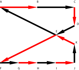
Figure 1: A configuration of $11$ points, $5$ lines, and $12$ directed segments in the real Euclidean plane, to which Eves’ Theorem applies.

The example shown in Figure 1, where eleven points lie on five lines, forming twelve directed segments, gives the general idea of Eves’ Theorem. The ratio of Euclidean signed distances

$$\frac{AB\cdot CD\cdot EF\cdot GH\cdot IJ\cdot KE}{BC\cdot DE\cdot FG\cdot HI\cdot JK\cdot EA}$$

is called (by Eves) an “h-expression,” meaning that each point $A,\ldots,K$ occurs equally many times in the numerator and denominator (for example, $E$ occurs twice), and each line defined by the two lists of six segments also occurs equally many times (for example, $\overleftrightarrow{FG}=\overleftrightarrow{HI}$ occurs twice in the numerator and twice in the denominator). The statement of Eves’ Theorem is that the value of an h-expression is an invariant under projective transformations of the plane. Related identities for products of distances have been known in projective geometry since at least [P], but it is convenient to attribute the above formulation to Eves.

The notion of h-expression can also be more visually conveyed in terms of coloring the configuration — an idea demonstrated at a 2011 talk by Marc Frantz [F₁]. Each point in the configuration of Figure 1 is an endpoint of an equal number of red and black segments, and, dually, each line contains an equal number of red and black segments. Then the ratio of the product of red lengths to the product of black lengths is Eves’ invariant.

Eves’ Theorem, when stated in a purely projective way (using homogeneous coordinates, not Euclidean distances, as in Example 4.16) is itself a special case of a family of invariant ratios of products of determinants of homogeneous coordinates for points in projective space over a field $\mathbb{K}$. These ratios were well-known in $19^{th}$ century Invariant Theory ([B], [C], [Salmon]), but have been more recently used (and, sometimes, re-discovered) in projective geometry applied to computational topics such as vision and photogrammetry, or automated proofs ([BB], [CRG], [F₂], [RG]).

Eves’ Theorem can be stated in terms of a function, where the input is a configuration of points $\mathcal{S}$ in projective space $\mathbb{K}P^{D}$, and the output is a ratio, i.e., an element of the projective line $\mathbb{K}P^{1}$; the content of the Theorem is that the ratio is well-defined (independent of certain choices made in specifying the configuration) and also invariant under projective transformations. Our new construction, Theorem 4.15, generalizes the target to a “weighted projective space” $\mathbb{K}P(p_{0},\ldots,p_{n})$, so the projective line is the special case $\mathbb{K}P(1,1)$. In Section 4, we give a unified treatment of the configurations to which Theorem 4.15 applies, by a weighting, coloring, and indexing scheme. A configuration $\mathcal{S}$ of points in the projective space $\mathbb{K}P^{D}$ that satisfies a condition (Definition 4.12), depending on the weight vector ${\mathbf{p}}=(p_{0},\ldots,p_{n})$, is assigned an element $E_{\mathbf{p}}(\mathcal{S})\in\mathbb{K}P({\mathbf{p}})$, an invariant under “morphisms” of the configuration (Definition 4.8), which generalize projective transformations. The number of colors is $n+1$, so the classical case is the assignment of Eves’ ratio $E_{(1,1)}(\mathcal{S})\in\mathbb{K}P(1,1)$ to some two-color configurations $\mathcal{S}$, and the new weighted invariants apply to a larger category of multi-color configurations.

In Section 2 we review the definition and some elementary properties of weighted projective spaces — these properties are well-known in the complex case, but the real case is different in some ways we intend to exploit, so we are careful to present all the necessary details. Section 3 introduces a new notion of “reconstructibility” for a weighted projective space; the two main results are that complex weighted projective spaces are all reconstructible, and that some real weighted projective spaces are not. In Section 5 we review a connection between real projective and Euclidean geometry, and state a Euclidean version of Theorem 4.15. Section 6 applies the notion of reconstructibility to show that in the complex case, the weighted invariant $E_{\mathbf{p}}$ of a multi-color configuration can be determined by finding the (classical) $E_{(1,1)}$ ratios for a finite list of related two-color configurations. However, in the real case, Examples 6.4, 6.5, 6.6 give pairs of configurations with different weighted invariants in $\mathbb{R}P({\mathbf{p}})$, but which cannot be distinguished by applying the reconstruction method to the $E_{(1,1)}$ ratios in $\mathbb{R}P^{1}$.

2 Weighted projective spaces

This Section reviews the definition of weighted projective spaces and some of their elementary properties. For the complex case, these properties (in particular, Examples 2.4 and 2.17), are well-known ([Delorme], [Dolgachev]); we give elementary proofs with the intent of showing how the complex and real cases are different. Only the objects’ set-theoretic properties are of interest here, not their structure as topological or analytic spaces, algebraic varieties, or orbifolds. The applications in subsequent Sections use only $\mathbb{R}$ and $\mathbb{C}$, but to start in a general way, let $\mathbb{K}$ be any field.

2.1 The basic construction

The ingredients are $n\in\mathbb{N}$, the vector space $\mathbb{K}^{n+1}$, and a weight ${\mathbf{p}}=(p_{0},p_{1},\ldots,p_{n})\in\mathbb{N}^{n+1}$. Denote $\mathbb{K}^{n+1}_{*}=\mathbb{K}^{n+1}\setminus\{\mathbf{0}\}$, and for elements ${\mathbf{z}}=(z_{0},\ldots,z_{n})$, $\mathbf{w}=(w_{0},\ldots,w_{n})\in\mathbb{K}^{n+1}_{*}$, define a relation $\sim_{\mathbf{p}}$ so that ${\mathbf{z}}\sim_{\mathbf{p}}{\mathbf{w}}$ means there exists $\lambda\in\mathbb{K}^{1}_{*}$ such that:

$$w_{0}=\lambda^{p_{0}}z_{0},\ \ w_{1}=\lambda^{p_{1}}z_{1},\ \ldots,\ w_{n}=\lambda^{p_{n}}z_{n}.$$

This is an equivalence relation on $\mathbb{K}^{n+1}_{*}$ because $\mathbb{K}$ is a field.

Definition 2.1.

Let $\mathbb{K}P({\mathbf{p}})$ denote the set of equivalence classes for $\sim_{\mathbf{p}}$. $\mathbb{K}P({\mathbf{p}})=\mathbb{K}P(p_{0},\ldots,p_{n})$ is the weighted projective space corresponding to the weight $\mathbf{p}$.

Notation 2.2.

Let $\pi_{\mathbf{p}}:\mathbb{K}^{n+1}_{*}\to\mathbb{K}P({\mathbf{p}})$ denote the canonical quotient map, defined so that $\pi_{\mathbf{p}}({\mathbf{z}})$ is the equivalence class of ${\mathbf{z}}$. It is convenient to use the same letter for elements of the weighted projective space, and square brackets for weighted homogeneous coordinates:

$$\pi_{\mathbf{p}}({\mathbf{z}})=z=[z_{0}:z_{1}:\ldots:z_{n}]_{\mathbf{p}}.$$

Example 2.3.

For ${\mathbf{p}}=(1,1,\ldots,1)$, $\mathbb{K}P(1,1,\ldots,1)$ is the usual projective space, denoted $\mathbb{K}P^{n}$, with homogeneous coordinates $\pi:(z_{0},\ldots,z_{n})\mapsto[z_{0}:\ldots:z_{n}]$ (omitting the subscripts).

Example 2.4.

For $\mathbb{K}=\mathbb{C}$ and ${\mathbf{p}}=(p,p,\ldots,p)$, ${\mathbf{z}}$ and ${\mathbf{w}}\in\mathbb{C}^{n+1}_{*}$ are $\sim_{\mathbf{p}}$-equivalent if and only if they are related by non-zero complex scalar multiplication, so the following sets are exactly equal: $\mathbb{C}P(p,p,\ldots,p)=\mathbb{C}P(1,1,\ldots,1)={\mathbb{C}}P^{n}$.

Example 2.5.

For $\mathbb{K}=\mathbb{R}$ and ${\mathbf{p}}=(2k+1,2k+1,\ldots,2k+1)$, ${\mathbf{z}}$ and ${\mathbf{w}}\in\mathbb{R}^{n+1}_{*}$ are $\sim_{\mathbf{p}}$-equivalent if and only if they are related by non-zero real scalar multiplication, so the following sets are exactly equal: $\mathbb{R}P(2k+1,2k+1,\ldots,2k+1)=\mathbb{R}P(1,1,\ldots,1)={\mathbb{R}}P^{n}$.

Example 2.6.

For $\mathbb{K}=\mathbb{R}$ and ${\mathbf{p}}=(2k,2k,\ldots,2k)$, the restriction of $\pi_{\mathbf{p}}$ to the unit sphere $S^{n}\subseteq\mathbb{R}^{n+1}_{*}$ is a one-to-one function onto $\mathbb{R}P({\mathbf{p}})$. It is not inconvenient to identify the sets: $\mathbb{R}P(2k,2k,\ldots,2k)=S^{n}$.

2.2 Mappings

Let $\mathbb{K}$ and $\mathbb{F}$ be fields, and let ${\mathbf{p}}\in\mathbb{N}^{n+1}$, ${\mathbf{q}}\in\mathbb{N}^{N+1}$ be weights. Consider any function $\mathbf{f}:\mathbb{K}^{n+1}_{*}\to\mathbb{F}^{N+1}$. Given $\mathbf{z}\in\mathbb{K}^{n+1}_{*}$, suppose $\mathbf{f}$ has the following two properties: first,

$$\mathbf{f}(\mathbf{z})=(w_{0},w_{1},\ldots,w_{N})\neq\mathbf{0},$$ (1)

and second, for any $\lambda\in\mathbb{K}^{1}_{*}$, there exists $\mu\in\mathbb{F}^{1}_{*}$ so that

$$\mathbf{f}(\lambda^{p_{0}}z_{0},\lambda^{p_{1}}z_{1},\ldots,\lambda^{p_{n}}z_{n})=(\mu^{q_{0}}w_{0},\mu^{q_{1}}w_{1},\ldots,\mu^{q_{N}}w_{N}).$$ (2)

Then $\mathbf{f}$ also has these two properties at every point ${\mathbf{z}^{\prime}}\in\mathbb{K}^{n+1}_{*}$ in the same equivalence class as ${\mathbf{z}}$, and if ${\mathbf{z}^{\prime}}\sim_{\mathbf{p}}{\mathbf{z}}$, then ${\mathbf{f}}({\mathbf{z}^{\prime}})\sim_{\mathbf{q}}{\mathbf{f}}({\mathbf{z}})$. Let ${\mathbf{U}}\subseteq\mathbb{K}^{n+1}_{*}$ be the set of points where $\mathbf{f}$ has the two properties, and let $U=\pi_{\mathbf{p}}({\mathbf{U}})$. Then we say “$\mathbf{f}$ induces a map from $\mathbb{K}P({\mathbf{p}})$ to $\mathbb{F}P({\mathbf{q}})$ which is well-defined on the set $U$,” and denote the induced map, which takes $\pi_{\mathbf{p}}(\mathbf{z})\in U$ to $\pi_{\mathbf{q}}({\mathbf{f}}({\mathbf{z}}))$, by $f:z\mapsto f(z)$. For $z\notin U$, $f(z)$ is undefined.

Lemma 2.7.

For $\mathbf{f}$, $f$, and $\mathbf{U}$ as above, and an element $w\in\mathbb{F}P({\mathbf{q}})$, let ${\mathbf{w}}\in\mathbb{F}^{N+1}_{*}$ be any representative ${\mathbf{w}}\in w=\pi_{\mathbf{q}}({\mathbf{w}})$. Then, the inverse image of $w$ is:

$$f^{-1}(w)=\pi_{\mathbf{p}}(\{{\mathbf{z}}\in{\mathbf{U}}:{\mathbf{f}}({\mathbf{z}})\sim_{\mathbf{q}}{\mathbf{w}}\}).$$ (3)

Proof.

The inverse image is

$$f^{-1}(w)=\{z\in\mathbb{K}P({\mathbf{p}}):z\in\pi_{\mathbf{p}}({\mathbf{U}})\mbox{ and }f(z)=w\}.$$

The first condition is that $\exists{\mathbf{x}}\in{\mathbf{U}}:z=\pi_{\mathbf{p}}({\mathbf{x}})$, and the second condition is that the $\sim_{\mathbf{q}}$-equivalence class of $\mathbf{w}$ is the same as the $\sim_{\mathbf{q}}$-equivalence class of ${\mathbf{f}}({\mathbf{z}})$ for some ${\mathbf{z}}\in z$. So,

$$f^{-1}(w)=\left\{z\in\mathbb{K}P({\mathbf{p}}):\left(\exists{\mathbf{x}}\in{\mathbf{U}}:{\mathbf{x}}\in z\right)\mbox{ and }\left(\exists{\mathbf{z}}\in z:{\mathbf{f}}({\mathbf{z}})\sim_{\mathbf{q}}{\mathbf{w}}\right)\right\}.$$

From (3), denote the RHS set (depending on $w$ but not the choice of $\mathbf{w}$):

$$A_{w} = \pi_{\mathbf{p}}(\{{\mathbf{z}}\in{\mathbf{U}}:{\mathbf{f}}({\mathbf{z}})\sim_{\mathbf{q}}{\mathbf{w}}\})$$

$$= \left\{z\in\mathbb{K}P({\mathbf{p}}):\exists{\mathbf{z}}\in{\mathbf{U}}:\left(\pi_{\mathbf{p}}({\mathbf{z}})=z\mbox{ and }{\mathbf{f}}({\mathbf{z}})\sim_{\mathbf{q}}{\mathbf{w}}\right)\right\}.$$

If $z\in A_{w}$, letting ${\mathbf{x}}={\mathbf{z}}$ shows $z\in f^{-1}(w)$. Conversely, if $z\in f^{-1}(w)$, then $\exists{\mathbf{x}}\in{\mathbf{U}}:{\mathbf{x}}\in z$ and $\exists{\mathbf{z}}\in z:{\mathbf{f}}({\mathbf{z}})\sim_{\mathbf{q}}{\mathbf{w}}$. Since ${\mathbf{x}}\in{\mathbf{U}}$ has properties (1) and (2), and ${\mathbf{z}}\sim_{\mathbf{p}}{\mathbf{x}}\in z$, $\mathbf{z}$ also has the two properties, so ${\mathbf{z}}\in{\mathbf{U}}$, and $z\in A_{w}$. ∎

Similar reasoning with the above data leads to the following equivalences:

Proposition 2.8.

A map $f:\mathbb{K}P({\mathbf{p}})\to\mathbb{F}P({\mathbf{q}})$ which is well-defined on the set $U$ is an onto map if and only if: for all ${\mathbf{w}}\in\mathbb{F}^{N+1}_{*}$, there exists ${\mathbf{z}}\in{\mathbf{U}}$ such that ${\mathbf{f}}({\mathbf{z}})\sim_{\mathbf{q}}{\mathbf{w}}$.  

Proposition 2.9.

A map $f:\mathbb{K}P({\mathbf{p}})\to\mathbb{F}P({\mathbf{q}})$ which is well-defined on the set $U$ is a one-to-one map if and only if: for all ${\mathbf{z}}$, ${\mathbf{z}^{\prime}}\in{\mathbf{U}}$, if ${\mathbf{f}}({\mathbf{z}})\sim_{\mathbf{q}}{\mathbf{f}}({\mathbf{z}^{\prime}})$, then ${\mathbf{z}}\sim_{\mathbf{p}}{\mathbf{z}^{\prime}}$.  

Example 2.10.

For $m\in\mathbb{N}$, consider two weights, ${\mathbf{q}}=(q_{0},q_{1},\ldots,q_{n})$ and ${\mathbf{p}}=(mq_{0},mq_{1},\ldots,mq_{n})$, and let ${\mathbf{f}}$ be the inclusion $\mathbb{K}^{n+1}_{*}\to\mathbb{K}^{n+1}:{\mathbf{z}}\mapsto{\mathbf{z}}$. ${\mathbf{f}}$ clearly satisfies (1) at every point ${\mathbf{z}}\in\mathbb{K}^{n+1}_{*}$, and also (2) with $\mu=\lambda^{m}$, so ${\mathbf{U}}=\mathbb{K}^{n+1}_{*}$. The induced map $f:\mathbb{K}P({\mathbf{p}})\to\mathbb{K}P({\mathbf{q}})$ is well-defined on $U=\mathbb{K}P({\mathbf{p}})$, and is an onto map as in Proposition 2.8. $f$ is also one-to-one if it satisfies the condition of Proposition 2.9: for all ${\mathbf{z}}$, ${\mathbf{z}^{\prime}}\in\mathbb{K}^{n+1}_{*}$, if $(z_{0}^{\prime},\ldots,z_{n}^{\prime})=(\lambda^{q_{0}}z_{0},\ldots,\lambda^{q_{n}}z_{n})$ for some $\lambda\in\mathbb{K}^{1}_{*}$, then there exists $\mu\in\mathbb{K}^{1}_{*}$ such that $(z_{0}^{\prime},\ldots,z_{n}^{\prime})=(\mu^{mq_{0}}z_{0},\ldots,\mu^{mq_{n}}z_{n})$. So, if $\mathbb{K}$ and $m$ have the property that $\forall\lambda\neq 0$ $\exists\mu:\mu^{m}=\lambda$, then $f$ is one-to-one; for example, this happens for $\mathbb{K}=\mathbb{C}$ and any $m$, and also for $\mathbb{K}=\mathbb{R}$ and odd $m$. Another situation in which $f$ is one-to-one is the case where $\mathbb{K}=\mathbb{R}$ and all the integers $q_{0}$, …, $q_{n}$ are even: for any $\lambda\neq 0$, let $\mu=|\lambda|^{1/m}$, then for $k=0,\ldots,n$, $\mu^{mq_{k}}=(|\lambda|^{1/m})^{mq_{k}}=|\lambda|^{q_{k}}=\lambda^{q_{k}}$.

In each of the cases mentioned in Example 2.10 where the induced map $f$ is one-to-one, we have ${\mathbf{z}}\sim_{\mathbf{p}}{\mathbf{z}^{\prime}}\iff{\mathbf{z}}\sim_{\mathbf{q}}{\mathbf{z}^{\prime}}$, so the equivalence classes are the same, $f$ is the identity map, and these sets are equal: $\mathbb{K}P({\mathbf{p}})=\mathbb{K}P({\mathbf{q}})$.

Example 2.11.

The inclusion ${\mathbf{f}}:\mathbb{R}^{n+1}_{*}\to\mathbb{R}^{n+1}$ as in Example 2.10 induces a well-defined, onto map $f:\mathbb{R}P(2,2,\ldots,2)\to\mathbb{R}P(1,1,\ldots,1)$, but $f$ is not one-to-one. This map $f$ is the usual two-to-one covering $S^{n}\to\mathbb{R}P^{n}$ (the “antipodal identification”).

Theorem 2.12.

For any weight ${\mathbf{q}}=(q_{0},\ldots,q_{n})$, let ${\mathbf{p}}=(2q_{0},\ldots,2q_{n})$. Let $f:\mathbb{R}P({\mathbf{p}})\to\mathbb{R}P({\mathbf{q}})$ be induced by the inclusion ${\mathbf{f}}$ as in Example 2.10. If $q_{j}$ is odd, then the restriction of $f$ to the set $\pi_{\mathbf{p}}(\{{\mathbf{z}}:z_{j}\neq 0\})$ is two-to-one.

Proof.

Take any ${\mathbf{w}}\in\mathbb{R}^{n+1}_{*}$ with $w_{j}\neq 0$, and let $w=\pi_{\mathbf{q}}({\mathbf{w}})$. By Lemma 2.7,

$$f^{-1}(w) = \pi_{\mathbf{p}}(\{{\mathbf{z}}\in\mathbb{R}^{n+1}_{*}:{\mathbf{z}}\sim_{\mathbf{q}}{\mathbf{w}}\})$$

$$= \pi_{\mathbf{p}}(\{(\mu^{q_{0}}w_{0},\ldots,\mu^{q_{n}}w_{n}):\mu\in\mathbb{R}^{1}_{*}\}).$$

Two points $(\mu_{1}^{q_{0}}w_{0},\ldots,\mu_{1}^{q_{n}}w_{n})$, $(\mu_{2}^{q_{0}}w_{0},\ldots,\mu_{2}^{q_{n}}w_{n})$ are $\sim_{\mathbf{p}}$-equivalent if and only if there exists $\lambda\in\mathbb{R}^{1}_{*}$ such that

$$\mu_{1}^{q_{0}}w_{0}=\lambda^{2q_{0}}\mu_{2}^{q_{0}}w_{0},\ldots,\mu_{1}^{q_{n}}w_{n}=\lambda^{2q_{n}}\mu_{2}^{q_{n}}w_{n}.$$ (4)

For $w_{j}\neq 0$ and $q_{j}$ odd, $\mu_{1}^{q_{j}}w_{j}=\lambda^{2q_{j}}\mu_{2}^{q_{j}}w_{j}\iff\lambda^{2}=\mu_{1}/\mu_{2}$, which is equivalent to the system of equations (4). So, the two points are $\sim_{\mathbf{p}}$-equivalent if and only if $\mu_{1}$ and $\mu_{2}$ have the same sign: there are two $\sim_{\mathbf{p}}$-equivalence classes. ∎

Example 2.13.

If all the $q_{j}$ are odd, then $f$ as in Theorem 2.12 is globally two-to-one. Example 2.11 is a special case. An example with the $q_{j}$ not all odd is the map $f:\mathbb{R}P(4,2)\to\mathbb{R}P(2,1)$. For this $f$, $f^{-1}([1:z_{1}]_{(2,1)})=\{[1:z_{1}]_{(4,2)},[1:-z_{1}]_{(4,2)}\}$, a two-element set for $z_{1}\neq 0$, but a singleton for $z_{1}=0$.

Example 2.14.

For $m\in\mathbb{N}$, consider two weights, ${\mathbf{q}}=(q_{0},q_{1},q_{2},\ldots,q_{n})$ and ${\mathbf{p}}=(q_{0},mq_{1},mq_{2},\ldots,mq_{n})$, and let ${\mathbf{f}}$ be the polynomial map

$${\mathbf{f}}:\mathbb{K}^{n+1}_{*}\to\mathbb{K}^{n+1}:(z_{0},z_{1},z_{2},\ldots,z_{n})\mapsto(z_{0}^{m},z_{1},z_{2},\ldots,z_{n}).$$

${\mathbf{f}}$ clearly satisfies (1) at every point ${\mathbf{z}}\in\mathbb{K}^{n+1}_{*}$, and also (2) with $\mu=\lambda^{m}$, so ${\mathbf{U}}=\mathbb{K}^{n+1}_{*}$. The induced map $f:\mathbb{K}P({\mathbf{p}})\to\mathbb{K}P({\mathbf{q}})$ is well-defined on $U=\mathbb{K}P({\mathbf{p}})$. $f$ is an onto map if it satisfies the condition of Proposition 2.8: for all ${\mathbf{w}}=(w_{0},\ldots,w_{n})\in\mathbb{K}^{n+1}_{*}$, there exist ${\mathbf{z}}$ and $\lambda$ such that $(w_{0},\ldots,w_{n})=(\lambda^{q_{0}}z_{0}^{m},\ldots,\lambda^{q_{n}}z_{n})$. For example, if $\mathbb{K}=\mathbb{C}$, or if $\mathbb{K}=\mathbb{R}$ and $m$ is odd, then given ${\mathbf{w}}$, one can choose $\lambda=1$, any $z_{0}$ with $z_{0}^{m}=w_{0}$, and $z_{k}=w_{k}$ for $k=1,\ldots,n$. Another situation in which $f$ is onto is the case where $\mathbb{K}=\mathbb{R}$ and $q_{0}$ is odd: for $w_{0}\geq 0$, make the same choices mentioned in the previous case, and for $w_{0}<0$, choose $\lambda=-1$, any $z_{0}$ with $z_{0}^{m}=(-1)^{q_{0}}w_{0}=|w_{0}|$, and $z_{k}=w_{k}/(-1)^{q_{k}}$ for $k=1,\ldots,n$.

Example 2.15.

The polynomial map ${\mathbf{f}}:\mathbb{R}^{2}_{*}\to\mathbb{R}^{2}:(z_{0},z_{1})\mapsto(z_{0}^{2},z_{1})$ induces a well-defined map $f:\mathbb{R}P(2,2)\to\mathbb{R}P(2,1)$ as in Example 2.14, but the induced map is not onto. The point $[-1:1]_{\mathbf{q}}$ is not in the image of $f$; there is no $(z_{0},z_{1})\in\mathbb{R}^{2}_{*}$ such that $(z_{0}^{2},z_{1})\sim_{\mathbf{q}}(-1,1)$.

Lemma 2.16.

For $w_{0}\in\mathbb{C}^{1}_{*}$, $N$, $P\in\mathbb{N}$, suppose $\{\zeta_{0},\ldots,\zeta_{N-1}\}$ are the $N$ distinct complex roots of the equation $\zeta^{N}=w_{0}$. Then the number of distinct elements in the set $\{\zeta_{0}^{P},\ldots,\zeta_{N-1}^{P}\}$ is $\mbox{\rm lcm}(P,N)/P$.

Proof.

In polar form, $w_{0}=\rho e^{i\theta}$ for a unique $\rho>0$, $\theta\in[0,2\pi)$. By re-labeling if necessary, $\zeta_{j}^{P}=\rho^{P/N}e^{i(\theta+2\pi j)P/N}$ for $j=0,\ldots,N-1$. Let $j$ be the smallest integer such that $jP/N\in\mathbb{N}$. It follows that $j=\mbox{\rm lcm}(P,N)/P$, the elements $\zeta_{k}^{P}$ are distinct for $k=0,\ldots,j-1$, and $\zeta_{k}^{P}=\zeta_{k+j}^{P}$. ∎

Example 2.17.

Let $\mathbb{K}=\mathbb{C}$. Consider a weight where $n$ of the $n+1$ integers have a common factor $m$ — without loss of generality, ${\mathbf{p}}=(q_{0},mq_{1},mq_{2},\ldots,mq_{n})$ as in Example 2.14. Suppose further that the integers $m$ and $q_{0}$ are relatively prime (have no common factor $>1$) — this can be achieved without changing the set $\mathbb{C}P({\mathbf{p}})$, by dividing out any common factor as in Example 2.10. Now let ${\mathbf{q}}=(q_{0},q_{1},q_{2},\ldots,q_{n})$; then the map ${\mathbf{f}}(z_{0},z_{1},z_{2},\ldots,z_{n})=(z_{0}^{m},z_{1},z_{2},\ldots,z_{n})$ from Example 2.14 induces a well-defined, onto map $f:\mathbb{C}P({\mathbf{p}})\to\mathbb{C}P({\mathbf{q}})$. It is also one-to-one: to establish this as in Proposition 2.9, we have to show that for any ${\mathbf{z}}$, ${\mathbf{z}^{\prime}}\in\mathbb{C}^{n+1}_{*}$, if there exists $\lambda\neq 0$ such that

$$(\lambda^{q_{0}}z_{0}^{m},\lambda^{q_{1}}z_{1},\ldots,\lambda^{q_{n}}z_{n})=((z_{0}^{\prime})^{m},z_{1}^{\prime},\ldots,z_{n}^{\prime}),$$ (5)

then there exists $\mu\neq 0$ so that

$$(\mu^{q_{0}}z_{0},\mu^{mq_{1}}z_{1},\ldots,\mu^{mq_{n}}z_{n})=(z_{0}^{\prime},z_{1}^{\prime},\ldots,z_{n}^{\prime}).$$ (6)

The algebra problem is: given $\lambda$, ${\mathbf{z}}$, ${\mathbf{z}^{\prime}}$, find $\mu$. If $z_{0}^{\prime}=0$, then $z_{0}=0$ and we can pick any $\mu$ satisfying $\mu^{m}=\lambda$. If $z_{0}^{\prime}\neq 0$, then $z_{0}\neq 0$, and there are $m$ different roots $\{\mu_{k}:k=0,\ldots,m-1\}$ satisfying $\mu_{k}^{m}=\lambda$. For $j=1,\ldots,n$, each $\mu_{k}$ satisfies $\mu_{k}^{mq_{j}}z_{j}=\lambda^{q_{j}}z_{j}=z_{j}^{\prime}$. Each $\mu_{k}$ also satisfies

$$(\mu_{k}^{q_{0}})^{m}=\mu_{k}^{mq_{0}}=\lambda^{q_{0}}=(z_{0}^{\prime})^{m}/z_{0}^{m}=(z_{0}^{\prime}/z_{0})^{m},$$

so each element of the set $R_{1}=\{\mu_{0}^{q_{0}},\ldots,\mu_{m-1}^{q_{0}}\}$ is also one of the $m$ elements of the set $R_{2}=\{\xi:\xi^{m}=(z_{0}^{\prime}/z_{0})^{m}\}$. One of the elements of $R_{2}$ is $z_{0}^{\prime}/z_{0}$. Using the assumption that $m$ and $q_{0}$ are relatively prime and Lemma 2.16, $R_{1}$ has $m$ distinct elements, so there is some $k$ such that $\mu_{k}^{q_{0}}=z_{0}^{\prime}/z_{0}$. This $\mu_{k}$ is the $\mu$ required in (6), to show $f$ is one-to-one.

Example 2.18.

Let $\mathbb{K}=\mathbb{R}$, and consider, as in Example 2.17, a weight ${\mathbf{p}}=(q_{0},mq_{1},mq_{2},\ldots,mq_{n}).$ Here we assume $m$ is odd but make no assumption on $q_{0}$. Now let ${\mathbf{q}}=(q_{0},q_{1},q_{2},\ldots,q_{n})$; then the map ${\mathbf{f}}(z_{0},z_{1},z_{2},\ldots,z_{n})=(z_{0}^{m},z_{1},z_{2},\ldots,z_{n})$ from Example 2.14 induces a well-defined, onto map $f:\mathbb{R}P({\mathbf{p}})\to\mathbb{R}P({\mathbf{q}})$. It is also one-to-one: the algebra problem is to solve the same equations (5), (6), for a real $\mu$ in terms of real ${\mathbf{z}}$, ${\mathbf{z}^{\prime}}$, $\lambda$. Given $\lambda\neq 0$, let $\mu$ be the unique real solution of $\mu^{m}=\lambda$. Then, for $j=1,\ldots,n$, $\mu^{mq_{j}}z_{j}=\lambda^{q_{j}}z_{j}=z_{j}^{\prime}$, and $(\mu^{q_{0}}z_{0})^{m}=\lambda^{q_{0}}z_{0}^{m}=(z_{0}^{\prime})^{m}\implies\mu^{q_{0}}z_{0}=z_{0}^{\prime}$.

Example 2.19.

Let $\mathbb{K}=\mathbb{R}$, and consider, as in Example 2.18, a weight ${\mathbf{p}}=(q_{0},mq_{1},mq_{2},\ldots,mq_{n}).$ Here we assume $m$ is even, $q_{0}$ is odd, and all $q_{1},\ldots,q_{n}$ are even. Now let ${\mathbf{q}}=(q_{0},q_{1},q_{2},\ldots,q_{n})$; then the map ${\mathbf{f}}(z_{0},z_{1},z_{2},\ldots,z_{n})=(z_{0}^{m},z_{1},z_{2},\ldots,z_{n})$ from Example 2.14 induces a well-defined, onto map $f:\mathbb{R}P({\mathbf{p}})\to\mathbb{R}P({\mathbf{q}})$. It is also one-to-one: the algebra problem is to solve (5), (6), for a real $\mu$ in terms of real ${\mathbf{z}}$, ${\mathbf{z}^{\prime}}$, $\lambda$. Given $\lambda\neq 0$, the equation $\mu^{m}=|\lambda|$ has exactly two real solutions, $\{\mu_{1}=|\lambda|^{1/m},\mu_{2}=-|\lambda|^{1/m}\}$. Then, for $k=1,2$, $j=1,\ldots,n$, $\mu_{k}^{mq_{j}}z_{j}=|\lambda|^{q_{j}}z_{j}=\lambda^{q_{j}}z_{j}=z_{j}^{\prime}$. For $k=1,2$, $(\mu_{k}^{q_{0}}z_{0})^{m}=|\lambda|^{q_{0}}z_{0}^{m}=|\lambda^{q_{0}}z_{0}^{m}|=(z_{0}^{\prime})^{m}$, so the set $\{\mu_{1}^{q_{0}}z_{0},\mu_{2}^{q_{0}}z_{0}=-\mu_{1}^{q_{0}}z_{0}\}$ is contained in the set $\{z_{0}^{\prime},-z_{0}^{\prime}\}$, and one of the two roots is the required $\mu$ satisfying $\mu^{q_{0}}z_{0}=z_{0}^{\prime}$.

Example 2.20.

For an even number $p_{1}$, the function ${\mathbf{f}}(z_{0},z_{1})=(z_{0}^{p_{1}},z_{1})$ induces a well-defined, onto map $f:\mathbb{R}P(1,p_{1})\to\mathbb{R}P(1,1)$ as in Example 2.14. The induced map is not one-to-one: ${\mathbf{f}}(0,1)=(0,1)\sim_{\mathbf{q}}{\mathbf{f}}(0,-1)=(0,-1)$, but $(0,1)\not\sim_{\mathbf{p}}(0,-1)$.

3 Reconstructibility

Given a weight ${\mathbf{p}}$, and two indices $i<j$ in $\{0,1,\ldots,n\}$, consider numbers $a_{ij}$, $b_{ij}\in\mathbb{N}$ and a mapping ${\mathbf{c}}_{ij}:\mathbb{K}^{n+1}_{*}\to\mathbb{K}^{2}$ defined by the formula

$${\mathbf{c}}_{ij}(z_{0},z_{1},\ldots,z_{i},\ldots,z_{j},\ldots,z_{n})=(z_{i}^{a_{ij}},z_{j}^{b_{ij}}).$$

The function ${\mathbf{c}}_{ij}$ satisfies (1) on the complement of the set $\{{\mathbf{z}}:z_{i}=z_{j}=0\}$, and if the products are equal: $p_{i}a_{ij}=p_{j}b_{ij}$, then it also satisfies (2) for weights ${\mathbf{p}}$ and ${\mathbf{q}}=(1,1)$.

Notation 3.1.

For ${\mathbf{p}}$, $a_{ij}$, $b_{ij}$ as above, the function ${\mathbf{c}}_{ij}$ induces a map

$$c_{ij}:\mathbb{K}P({\mathbf{p}}) \to \mathbb{K}P^{1}:$$

$$\left[z_{0}:z_{1}:\ldots:z_{i}:\ldots:z_{j}:\ldots:z_{n}\right]_{\mathbf{p}} \mapsto \left[z_{i}^{a_{ij}}:z_{j}^{b_{ij}}\right],$$

which is well-defined on the complement of the set $\{[z_{0}:\ldots:z_{n}]_{\mathbf{p}}:z_{i}=z_{j}=0\}$. We call such a map an axis projection.

Lemma 3.2.

Given a weight $\mathbf{p}$ and indices $i$, $j$, let $\ell_{ij}=\mbox{\rm lcm}(p_{i},p_{j})$. Then

$$h_{ij}:\mathbb{K}P({\mathbf{p}})\to\mathbb{K}P^{1}:z\mapsto[z_{i}^{\ell_{ij}/p_{i}}:z_{j}^{\ell_{ij}/p_{j}}]$$ (7)

is an axis projection. For any axis projection $c_{ij}$ as in Notation 3.1, there exists $k_{ij}\in\mathbb{N}$ such that $c_{ij}$ factors as $c_{ij}=G_{ij}\circ h_{ij}$, where the function

$$G_{ij}:\mathbb{K}P^{1}\to\mathbb{K}P^{1}:[w_{0}:w_{1}]\mapsto[w_{0}^{k_{ij}}:w_{1}^{k_{ij}}]$$

is well-defined on $\mathbb{K}P^{1}$.

Proof.

$\ell_{ij}$ is the least common multiple of $p_{i}$ and $p_{j}$. By elementary number theory ([O] Ch. 3), any other common multiple is divisible by $\ell_{ij}$, so there exists $k_{ij}$ so that $p_{i}a_{ij}=p_{j}b_{ij}=k_{ij}\ell_{ij}$. ∎

Notation 3.3.

Let $I$ be the set of index pairs $\{(i,j):0\leq i<j\leq n\}$. Let $D_{\mathbf{p}}\subseteq\mathbb{K}P({\mathbf{p}})$ be the set of points where all the coordinates are non-zero: $\{z_{0}\neq 0,\ z_{1}\neq 0,\ \ldots,$ and $z_{n}\neq 0\}$. Given axis projections $c_{ij}$ for $(i,j)\in I$, let $\displaystyle{\prod c_{ij}}$ denote the map

$$\mathbb{K}P({\mathbf{p}}) \to \mathbb{K}P^{1}\times\mathbb{K}P^{1}\times\cdots\times\mathbb{K}P^{1}$$

$$z \mapsto \left(c_{11}(z),c_{12}(z),\ldots,c_{ij}(z),\ldots,c_{n-1,n}(z)\right).$$

The target space in the above Notation has one $\mathbb{K}P^{1}$ factor for each of the elements of $I$ ($\#I=n(n+1)/2$), so the output formula lists an axis projection for every index pair $(i,j)$. The map $\displaystyle{\prod c_{ij}}$ is well-defined at every point in $D_{\mathbf{p}}$, and possibly at some points not in $D_{\mathbf{p}}$.

Definition 3.4.

A weighted projective space $\mathbb{K}P({\mathbf{p}})$ is reconstructible means: there exist axis projections such that the restriction of the map $\displaystyle{\prod c_{ij}}$ to the domain $D_{\mathbf{p}}$ is one-to-one.

The idea is to try to use a list of unweighted ratios, $c_{ij}(z)$, as a coordinatization of the weighted projective space $\mathbb{K}P({\mathbf{p}})$. A reconstructible space is one where any point $z$ (with non-zero coordinates) can be uniquely “reconstructed” from a list of its values under some axis projections. The use of the domain $D_{\mathbf{p}}$ in the Definition omits consideration of points $z$ with a zero coordinate; as already seen in Examples 2.13 and 2.20, such points can exhibit exceptional behavior, and we are interested in properties of generic points.

Lemma 3.5.

Given ${\mathbf{p}}$, the following are equivalent.

1. $\mathbb{K}P({\mathbf{p}})$ is reconstructible;

2. for the axis projections $h_{ij}$ from (7), the map $\displaystyle{\prod_{(i,j)\in I}h_{ij}}$ is one-to-one on $D_{\mathbf{p}}$;

3. there exist a subset $J\subseteq I$ and axis projections $c_{ij}$ so that $\displaystyle{\prod_{(i,j)\in J}c_{ij}}$ is one-to-one on $D_{\mathbf{p}}$;

4. there exists a subset $J\subseteq I$ so that $\displaystyle{\prod_{(i,j)\in J}h_{ij}}$ is one-to-one on $D_{\mathbf{p}}$.

Proof.

The implications ${\mathit{2}}\implies{\mathit{1}}\implies{\mathit{3}}$ and ${\mathit{2}}\implies{\mathit{4}}\implies{\mathit{3}}$ are logically trivial. To show ${\mathit{3}}\implies{\mathit{2}}$, given $c_{ij}$ for $J\subseteq I$, pick any axis projections $c_{ij}$ for the remaining indices not in $J$; then

$${\prod_{(i,j)\in J}c_{ij}=F\circ\prod_{(i,j)\in I}c_{ij}},$$

where $F:(\mathbb{K}P^{1})^{\#I}\to(\mathbb{K}P^{1})^{\#J}$ forgets entries with non-$J$ indices. Then, by Lemma 3.2, there exist factorizations $c_{ij}=G_{ij}\circ h_{ij}$, so

$$\prod_{(i,j)\in J}c_{ij}=F\circ\left(\prod_{(i,j)\in I}G_{ij}\right)\circ\left(\prod_{(i,j)\in I}h_{ij}\right)$$

(where the product map $\displaystyle{\prod G_{ij}}:(\mathbb{K}P^{1})^{\#I}\to(\mathbb{K}P^{1})^{\#I}$ is defined in the obvious way for the composition to make sense). If $\displaystyle{\prod h_{ij}}$ is not one-to-one on $D_{\mathbf{p}}$, then $\displaystyle{\prod_{(i,j)\in J}c_{ij}}$ is also not one-to-one on $D_{\mathbf{p}}$. ∎

Example 3.6.

For any field $\mathbb{K}$, the space $\mathbb{K}P(1,p_{1},\ldots,p_{n})$ is reconstructible. Only $n$ axis projections are needed for a one-to-one product map: let $J=\{(0,j):j=1,\ldots,n\}$, and consider ${\mathbf{h}}_{0j}(z_{0},z_{1},\ldots,z_{n})=(z_{0}^{p_{j}},z_{j})$. If $z=\pi_{\mathbf{p}}({\mathbf{z}})$, $z^{\prime}=\pi_{\mathbf{p}}({\mathbf{z}^{\prime}})\in D_{\mathbf{p}}$ satisfy ${\mathbf{h}}_{0j}({\mathbf{z}})\sim_{(1,1)}{\mathbf{h}}_{0j}({\mathbf{z}^{\prime}})$ for $j=1,\ldots,n$, then there exist $\lambda_{0j}\neq 0$ such that $(z_{0}^{\prime})^{p_{j}}=\lambda_{0j}z_{0}^{p_{j}}$ and $z_{j}^{\prime}=\lambda_{0j}z_{j}$. Let $\mu=z_{0}^{\prime}/z_{0}$ (using the assumption that $z_{0}\neq 0$); then $\mu z_{0}=z_{0}^{\prime}$ and $\mu^{p_{j}}z_{j}=(z_{0}^{\prime}/z_{0})^{p_{j}}z_{j}=\lambda_{0j}z_{j}=z_{j}^{\prime}$, so ${\mathbf{z}}\sim_{\mathbf{p}}{\mathbf{z}^{\prime}}$.

Example 3.7.

Example 3.6 shows $\mathbb{R}P(1,p_{1})$ is reconstructible. Even though the map $h_{01}([z_{0}:z_{1}]_{\mathbf{p}})=[z_{0}^{p_{1}}:z_{1}]$ is not globally one-to-one when $p_{1}$ is even, as shown in Example 2.20, it is one-to-one when restricted to $D_{\mathbf{p}}$.

Example 3.8.

If one of the numbers $p_{0}$, $p_{1}$ is odd, then $\mathbb{R}P(p_{0},p_{1})$ is reconstructible. WLOG, let $p_{0}$ be odd. For the axis projection $c_{01}([z_{0}:z_{1}]_{\mathbf{p}})=[z_{0}^{p_{1}}:z_{1}^{p_{0}}]$, the following diagram is commutative. The label on the left arrow means that the indicated map is induced by the polynomial map $\mathbb{R}^{2}_{*}\to\mathbb{R}^{2}:(z_{0},z_{1})\mapsto(z_{0},z_{1}^{p_{0}})$.

The map on the left is globally one-to-one as in Example 2.18, and takes $D_{(p_{0},p_{1})}$ to $D_{(1,p_{1})}$. The lower right map is one-to-one on $D_{(1,p_{1})}$: either by Example 2.18 for odd $p_{1}$, or by Example 3.7 for even $p_{1}$.

Example 3.9.

If both $p_{0}$ and $p_{1}$ are even, then $\mathbb{R}P(p_{0},p_{1})$ is not reconstructible. Consider an axis projection induced by ${\mathbf{c}}_{01}(z_{0},z_{1})=(z_{0}^{a},z_{1}^{b})$. By Lemma 3.5, we may assume that $a$ and $b$ are not both even. If $a$ and $b$ are both odd, then ${\mathbf{c}}_{01}(1,1)=(1,1)\sim_{(1,1)}{\mathbf{c}}_{01}(-1,-1)=(-1,-1)$, but $(1,1)\not\sim_{\mathbf{p}}(-1,-1)$, so $c_{01}$ is not one-to-one. If $a$ is even and $b$ is odd (the remaining case being similar), then ${\mathbf{c}}_{01}(1,-1)=(1,-1)\sim_{(1,1)}{\mathbf{c}}_{01}(-1,-1)=(1,-1)$, but $(1,-1)\not\sim_{\mathbf{p}}(-1,-1)$, so again $c_{01}$ is not one-to-one.

Theorem 3.10.

For $\mathbb{K}=\mathbb{C}$ and any weight $\mathbf{p}$, $\mathbb{C}P({\mathbf{p}})$ is reconstructible.

Proof.

Case 1: $n=1$. Any space $\mathbb{C}P(q_{0},q_{1})$ is reconstructible (in fact, a stronger result holds: there is an axis projection which is one-to-one on the entire space). Let $g_{01}=\gcd(q_{0},q_{1})$ and $\ell_{01}=\mbox{\rm lcm}(q_{0},q_{1})$, so $q_{0}=g_{01}p_{0}$, $q_{1}=g_{01}p_{1}$, and $\ell_{01}=g_{01}p_{0}p_{1}$, where $p_{0}$, $p_{1}$ are relatively prime. The map

$${\mathbf{h}}_{01}:\mathbb{C}^{2}_{*}\to\mathbb{C}^{2}:(z_{0},z_{1})\mapsto(z_{0}^{\ell_{01}/q_{0}},z_{1}^{\ell_{01}/q_{1}})=(z_{0}^{p_{1}},z_{1}^{p_{0}})$$

induces an axis projection $h_{01}$ as in (7), so that the following diagram is commutative.

The left arrow, labeled $Id$, represents the identity map as in Example 2.10 with $m=g_{01}$. The map indicated by the lower arrow is induced by the polynomial map $\mathbb{C}^{2}_{*}\to\mathbb{C}^{2}:(z_{0},z_{1})\mapsto(z_{0}^{p_{1}},z_{1})$. Both maps, indicated by the lower and right arrows, are (globally) one-to-one as in Example 2.17, so we can conclude $h_{01}$ is one-to-one on the entire domain $\mathbb{C}P(q_{0},q_{1})$.

Case 2: $n>1$. We use a product of axis projections as in statement $\mathit{2}$. from Lemma 3.5. For $(i,j)\in I$, recall the notation $\ell_{ij}=\mbox{\rm lcm}(p_{i},p_{j})$, and fix

$$a_{ij}=\ell_{ij}/p_{i},\ \ \ b_{ij}=\ell_{ij}/p_{j},$$ (8)

and $g_{ij}=\gcd(p_{i},p_{j})$. Consider the product map

$$\prod_{(i,j)\in I}h_{ij}:[z_{0}:\ldots:z_{n}]_{\mathbf{p}}\mapsto\prod_{(i,j)\in I}[z_{i}^{a_{ij}}:z_{j}^{b_{ij}}].$$ (9)

To show this product map is one-to-one on $D_{\mathbf{p}}$, suppose we are given ${\mathbf{z}}$, ${\mathbf{z}^{\prime}}$ (with no zero components), and constants $\lambda_{ij}\in\mathbb{C}^{1}_{*}$ such that $\lambda_{ij}(z_{i}^{\prime})^{a_{ij}}=z_{i}^{a_{ij}}$ and $\lambda_{ij}(z_{j}^{\prime})^{b_{ij}}=z_{j}^{b_{ij}}$. The algebra problem is then to find $\mu\in\mathbb{C}^{1}_{*}$ such that

$$\mu^{p_{j}}z_{j}^{\prime}=z_{j}\mbox{\ \ \ for $j=0,\ldots,n$.}$$ (10)

There are $p_{0}$ distinct elements $\{\mu_{k},k=0,\ldots,p_{0}-1\}$ satisfying $\mu_{k}^{p_{0}}=z_{0}/z_{0}^{\prime}$. For each $k$ and for any $j=1,\ldots,n$,

$$(\mu_{k}^{p_{j}}z_{j}^{\prime})^{b_{0j}} = \mu_{k}^{p_{j}b_{0j}}(z_{j}^{\prime})^{b_{0j}}=\mu_{k}^{p_{0}a_{0j}}(z_{j}^{\prime})^{b_{0j}}$$ (11)

$$= \left(\frac{z_{0}}{z_{0}^{\prime}}\right)^{a_{0j}}(z_{j}^{\prime})^{b_{0j}}=\lambda_{0j}(z_{j}^{\prime})^{b_{0j}}=z_{j}^{b_{0j}}.$$

By Lemma 2.16,

$$\#\{\mu_{k}^{p_{j}}z_{j}^{\prime}:k=0,\ldots,p_{0}-1\}=\#\{\mu_{k}^{p_{j}}\}=\frac{\mbox{\rm lcm}(p_{0},p_{j})}{p_{j}}=\frac{\ell_{0j}}{p_{j}}=b_{0j},$$

which is equal to the number of roots in $\{\xi:\xi^{b_{0j}}=z_{j}^{b_{0j}}\}$, and so for each $j=1,\ldots,n$, there exists some index $k_{j}$ such that $\mu_{k_{j}}^{p_{j}}z_{j}^{\prime}=z_{j}$. At this point we note that if all the $k_{1},\ldots,k_{n}$ index values were the same, $\mu=\mu_{k_{j}}$ would satisfy (10) and we would be done. One case where this happens in a trivial way is $p_{0}=1$; this was already observed in Example 3.6.

The rest of the Proof does not attempt to show the $k_{j}$ values are equal to each other; instead we use their existence to establish the existence of some other index $x$ such that $\mu_{x}$ is the required solution of (10).

For $i,j=1,\ldots,n$ with $i<j$, $\mu_{k_{i}}$ and $\mu_{k_{j}}$ satisfy:

$$(\mu_{k_{i}}^{p_{i}}z_{i}^{\prime})^{a_{ij}} = \mu_{k_{i}}^{\ell_{ij}}(z_{i}^{\prime})^{a_{ij}}=z_{i}^{a_{ij}}=\lambda_{ij}(z_{i}^{\prime})^{a_{ij}},$$

$$(\mu_{k_{j}}^{p_{j}}z_{j}^{\prime})^{b_{ij}} = \mu_{k_{j}}^{\ell_{ij}}(z_{j}^{\prime})^{b_{ij}}=z_{j}^{b_{ij}}=\lambda_{ij}(z_{j}^{\prime})^{b_{ij}}$$

$$\implies\lambda_{ij} = \mu_{k_{i}}^{\ell_{ij}}=\mu_{k_{j}}^{\ell_{ij}}.$$ (12)

By re-labeling the roots if necessary, as in the Proof of Lemma 2.16, we may assume $\mu_{k}=r^{1/p_{0}}e^{i(\theta+2\pi k)/p_{0}}$ for $k=0,\ldots,p_{0}-1$. Then (12) implies the congruence

$$k_{j}\ell_{ij}\equiv k_{i}\ell_{ij}\mod p_{0}.$$ (13)

We are looking for an index $x$ such that for every $j=1,\ldots,n$, $\mu_{x}^{p_{j}}=\mu_{k_{j}}^{p_{j}}$, so $x$ is an integer solution to the following system of linear congruences, where $p_{j}$ and $k_{j}$ are known:

$$xp_{j}\equiv k_{j}p_{j}\mod p_{0}\mbox{\ \ \ for $j=1,\ldots,n$.}\\$$ (14)

Dividing each congruence by $\gcd(p_{0},p_{j})$ does not change the solution set:

$$\frac{xp_{j}}{g_{0j}} \equiv \frac{k_{j}p_{j}}{g_{0j}}\mod\frac{p_{0}}{g_{0j}}$$

$$\iff a_{0j}x \equiv a_{0j}k_{j}\mod b_{0j},$$

which is equivalent, since $a_{0j}$ and $b_{0j}$ are relatively prime, to:

$$x\equiv k_{j}\mod b_{0j}.$$ (15)

By (an elementary generalization of) the Chinese Remainder Theorem ([O], Thm. 10–4), there exists an integer solution $x$ of the system (15) if and only if for all pairs $1\leq i<j\leq n$,

$$k_{i}\equiv k_{j}\mod\gcd(b_{0i},b_{0j}).$$ (16)

Property (16) follows from (13): each congruence (16) is equivalent to

$$k_{i}\ell_{ij}\equiv k_{j}\ell_{ij}\mod\gcd(b_{0i},b_{0j})\ell_{ij}.$$

The following equalities are elementary ([O] Chs. 3, 5); one step uses the property that $a_{ij}$ and $b_{ij}$ are relatively prime:

$$\gcd(b_{0i},b_{0j})\ell_{ij} = \gcd(b_{0i}\ell_{ij},b_{0j}\ell_{ij})=\gcd(b_{0i}p_{i}a_{ij},b_{0j}p_{j}b_{ij})$$

$$= \gcd(\ell_{0i}a_{ij},\ell_{0j}b_{ij})=\gcd(\ell_{0i},\ell_{0j})$$

$$= \gcd(\mbox{\rm lcm}(p_{0},p_{i}),\mbox{\rm lcm}(p_{0},p_{j}))=\mbox{\rm lcm}(p_{0},\gcd(p_{i},p_{j}))$$

$$= \mbox{\rm lcm}(p_{0},g_{ij}).$$

By definition, $\ell_{ij}$ is a multiple of $g_{ij}$, and by (13), $k_{i}\ell_{ij}-k_{j}\ell_{ij}$ is a multiple of $p_{0}$. It follows that $k_{i}\ell_{ij}-k_{j}\ell_{ij}$ is a common multiple of $p_{0}$ and $g_{ij}$, and so a multiple of $\mbox{\rm lcm}(p_{0},g_{ij})$, which implies (16). ∎

Theorem 3.11.

For $\mathbb{K}=\mathbb{R}$, $\mathbb{R}P({\mathbf{p}})$ is reconstructible if and only if $p_{0},\ldots,p_{n}$ are not all even.

Proof.

To establish reconstructibility, assume, WLOG, $p_{0}$ is odd. We can proceed with the same notation as Case 2 of the Proof of Theorem 3.10, and use a product of axis projections as in (9), although as in Example 3.6, only $n$ axis projections, indexed by $(i,j)=(0,j)$, are needed for a one-to-one product map. Given real $\mathbf{z}$, ${\mathbf{z}^{\prime}}$, and $\lambda_{0j}$, the algebra problem is to find a real solution $\mu$ of Equation (10). Since $p_{0}$ is odd and $z_{0}\neq 0$, the equation $\mu^{p_{0}}z_{0}^{\prime}=z_{0}$ has a unique real solution for $\mu$. For each $j$, $b_{0j}=p_{0}/g_{0j}$ is odd, and using the unique solution for $\mu$ in Equation (11) gives $(\mu^{p_{j}}z_{j}^{\prime})^{b_{0j}}=z_{j}^{b_{0j}}$, which implies $\mu^{p_{j}}z_{j}^{\prime}=z_{j}$, so Equation (10) is satisfied.

For the converse, suppose $p_{j}=2^{e_{j}}q_{j}$ with $e_{j}>0$ and $q_{j}$ odd for $j=0,\ldots,n$. To show statement $\mathit{2}.$ from Lemma 3.5 is false, we show that the product of axis projections as in (7), (9) is exactly two-to-one on $D_{\mathbf{p}}$; let this map be denoted by the top arrow in the diagram below. WLOG, assume $e_{0}$ is the smallest of the $e_{j}$ exponents. By Example 2.10, dividing the weight $p$ by $m=2^{e_{0}-1}$ does not change the weighted projective space; this identity map is shown as the left arrow in the diagram.

The lower arrow is the map from Theorem 2.12; it is induced by the inclusion $\mathbb{R}^{n+1}_{*}\to\mathbb{R}^{n+1}$, and is two-to-one on the set $\{z:z_{0}\neq 0\}$, which contains $D_{\mathbf{p}}$. The upward arrow on the right is defined as in statement $\mathit{2}.$ from Lemma 3.5; this was shown to be one-to-one on $D_{(q_{0},\ldots,2^{e_{n}-e_{0}}q_{n})}$ in the first part of this Proof. The diagram is commutative (the top arrow is the composite of the other arrows) because the axis projections use the same exponents. For the top arrow,

$$a_{ij} = \frac{\mbox{\rm lcm}(p_{i},p_{j})}{p_{i}}=\frac{\mbox{\rm lcm}(2^{e_{i}}q_{i},2^{e_{j}}q_{j})}{2^{e_{i}}q_{i}}$$

$$= \frac{\mbox{\rm lcm}(2^{e_{i}-e_{0}}q_{i},2^{e_{j}-e_{0}}q_{j})2^{e_{0}}}{2^{e_{i}}q_{i}}.$$

For the right arrow, the corresponding exponent is

$$\frac{\mbox{\rm lcm}(2^{e_{i}-e_{0}}q_{i},2^{e_{j}-e_{0}}q_{j})}{2^{e_{i}-e_{0}}q_{i}},$$

which is the same, and similarly for the exponents $b_{ij}$. ∎

4 Generalizing Eves’ Theorem

4.1 Configurations in projective space

We begin with some combinatorial notation that is needed to keep track of various indexings.

Notation 4.1.

Two ordered $N$-tuples

$$(x_{1},\ldots,x_{N}),\ (y_{1},\ldots,y_{N})$$

are equivalent up to re-ordering if there exists a permutation $\sigma$ of the index set $\{1,\ldots,N\}$ such that $y_{i}=x_{\sigma(i)}$ for $i=1,\ldots,N$. This is an equivalence relation; we denote the equivalence class of $(x_{1},\ldots,x_{N})$ with square brackets, $[x_{1},\ldots,x_{N}]$, and call it an unordered list.

When it is necessary to index the entries in an unordered list, it is convenient to first pick an ordered representative. Using the following notation, we describe some configurations of points in (non-weighted) projective space.

Notation 4.2.

Given $D,r\in\mathbb{N}$, and points $\alpha_{1},\ldots,\alpha_{e},\ldots,\alpha_{r}\in\mathbb{K}P^{D}$, denote an ordered $r$-tuple of points

$$\vec{s}=(\alpha_{1},\ldots,\alpha_{e},\ldots,\alpha_{r}).$$

Such an ordered $r$-tuple is an independent $r$-tuple means: there exist representatives for the points, ${\mbox{\boldmath$\alpha$}}_{1},\ldots,{\mbox{\boldmath$\alpha$}}_{e},\ldots,{\mbox{\boldmath$\alpha$}}_{r}$, which form an independent set of $r$ vectors in $\mathbb{K}^{D+1}$ (so $r\leq D+1$). In the case $r=2$, we call the ordered, independent pair $\vec{s}=(\alpha,\beta)$ a directed segment, and the two points its endpoints. In the case $r=3$, ordered, independent triples are triangles $\vec{s}=\triangle(\alpha\beta\gamma)$.

Definition 4.3.

Given an independent $r$-tuple $\vec{s}$, there is a unique $r$-dimensional subspace ${\mathbf{L}}$ of $\mathbb{K}^{D+1}$ that is spanned by any independent set of representatives for the points in $\vec{s}$. The image $\pi({\mathbf{L}}\setminus\vec{0})=L$ is a $(r-1)$-dimensional projective subspace of $\mathbb{K}P^{D}$, which we call the span of $\vec{s}$.

It is convenient to also refer to the $\mathbb{K}$-linear subspace $\mathbf{L}$ as $\pi^{-1}(L)$, and to $L=\pi({\mathbf{L}})$, even though $\pi$ is not defined at $\vec{0}$.

Definition 4.4.

Given a weight ${\mathbf{p}}=(p_{0},\ldots,p_{n})$ as in Section 2 and some other numbers $D,\ell,r\in\mathbb{N}$ with $r\leq D+1$, a $({\mathbf{p}},r,\ell,D)$-configuration (or, just “configuration” when the ${\mathbf{p}}$, $r$, $\ell$, and $D$ are understood) is an ordered $(n+1)$-tuple $\mathcal{S}$,

$$\mathcal{S}=(\mathcal{S}_{0},\ldots,\mathcal{S}_{c},\ldots,\mathcal{S}_{n}),$$ (17)

where each $\mathcal{S}_{c}$ is an unordered list (possibly with repeats) of $\ell\cdot p_{c}$ ordered, independent $r$-tuples of points in $\mathbb{K}P^{D}$:

$$\mathcal{S}_{c}=[\vec{s}_{c}^{1},\ldots,\vec{s}_{c}^{\ \ell p_{c}}].$$

We remark that it is possible for some $\mathcal{S}$ to be both a $({\mathbf{p}},r,\ell,D)$-configuration and a $({\mathbf{p}^{\prime}},r,\ell^{\prime},D)$-configuration with ${\mathbf{p}}\neq{\mathbf{p}^{\prime}}$ and $\ell\neq\ell^{\prime}$, although if ${\mathbf{p}}$ is given, then $\ell$ is determined by the length of the lists $\mathcal{S}_{c}$.

As an aid to visualization and drawing, the indices $c=0,\ldots,n$ can correspond to colors: $c=0=$ black, $c=1=$ red, $c=2=$ green, etc. So, for $r=2$, $\mathcal{S}_{0}$ is a list of $\ell p_{0}$ black segments, $\mathcal{S}_{1}$ is a list of $\ell p_{1}$ red segments, etc.

Notation 4.5.

Given a $({\mathbf{p}},r,\ell,D)$-configuration $\mathcal{S}$, define the following sets:

• $\mathcal{P}(\mathcal{S})$ is the set of points $z\in\mathbb{K}P^{D}$ such that $z$ is one of the $r$ components of some $\vec{s}_{c}^{K}$ in $\mathcal{S}_{c}$, for some $c=0,\ldots,n$;

• $\mathcal{L}(\mathcal{S})$ is the set of $(r-1)$-dimensional projective subspaces which are the spans of the $r$-tuples $\vec{s}_{c}^{K}$;

• $\mathcal{U}(\mathcal{S})$ is the following union of $r$-dimensional subspaces in $\mathbb{K}^{D+1}$:

  $${\mathcal{U}(\mathcal{S})=\bigcup_{L\in\mathcal{L}(\mathcal{S})}\pi^{-1}(L)}.$$

All three sets depend only on the set of $r$-tuples in $\mathcal{S}$, not on the ordering in (17), nor on $\mathbf{p}$ and $\ell$.

For example, when $r=2$, any directed segment lies on a unique projective line, so $\mathcal{L}(\mathcal{S})$ is a (finite) set of projective lines in $\mathbb{K}P^{D}$. Since the same point may appear in several different $r$-tuples, it is possible for the size of $\mathcal{P}(\mathcal{S})$ to be small compared to the number of $r$-tuples.

Definition 4.6.

Given a $({\mathbf{p}},r,\ell,D)$-configuration $\mathcal{S}$, for $c=0,\ldots,n$, choose an ordered representative

$$S_{c}=(\vec{s}_{c}^{1},\ldots,\vec{s}_{c}^{K},\ldots,\vec{s}_{c}^{\ \ell p_{c}})$$ (18)

of the equivalence class $\mathcal{S}_{c}$. Define the $c$-degree of a point $z\in\mathbb{K}P^{D}$ to be

$$deg_{c}(z)=\#\{K:z\mbox{ is one of the $r$ points of the $r$-tuple }\vec{s}_{c}^{K}\mbox{ in }S_{c}\}.$$

According to the color scheme indexed by $c$, every point in the configuration has a black degree, a red degree, etc. Definition 4.6 is stated in a way so that possibly repeated $r$-tuples are counted with multiplicity. The assumption that each $r$-tuple is independent implies that $z$ appears at most once in an $r$-tuple. The number $deg_{c}(z)$ does not depend on the choice of ordered representative $S_{c}$ for $\mathcal{S}_{c}$, nor on ${\mathbf{p}}$ and $\ell$ if $\mathcal{S}$ admits another description as a $({\mathbf{p}^{\prime}},r,\ell^{\prime},D)$-configuration. For all but finitely many points in $\mathbb{K}P^{D}$, the $c$-degree is zero.

The following Definition is dual to Definition 4.6.

Definition 4.7.

For $\mathcal{S}$ and $S_{c}$ as in Definition 4.6, define the $c$-degree of a projective $(r-1)$-subspace $L$ of $\mathbb{K}P^{D}$ to be

$$deg_{c}(L)=\#\{K:\mbox{all $r$ points of the $r$-tuple }\vec{s}_{c}^{K}\mbox{ in }S_{c}\mbox{ lie on }L\}.$$

The following Definition of a morphism of a configuration was motivated by, but is different from, a notion of isomorphic plane configurations considered by [Shephard].

Definition 4.8.

Given a $({\mathbf{p}},r,\ell,D)$-configuration $\mathcal{S}=(\mathcal{S}_{0},\ldots,\mathcal{S}_{n})$, and a $({\mathbf{p}},r,\ell,D^{\prime})$-configuration $\mathcal{T}=(\mathcal{T}_{0},\ldots,\mathcal{T}_{n})$, $\mathcal{A}$ is a morphism from $\mathcal{S}$ to $\mathcal{T}$ means $\mathcal{A}$ is a function $\mathcal{P}(\mathcal{S})\to\mathcal{P}(\mathcal{T})$ such that:

1. For indexing purposes, for any ordered representative for each $\mathcal{S}_{c}$, $c=0,\ldots,n$,

   $$(\vec{s}_{c}^{1},\ldots,\vec{s}_{c}^{K},\ldots,\vec{s}_{c}^{\ \ell p_{c}}),$$ (19)

   there is an ordered representative for $\mathcal{T}_{c}$,

   $$(\vec{t}_{c}^{\ 1},\ldots,\vec{t}_{c}^{\ K},\ldots,\vec{t}_{c}^{\ \ell p_{c}}),$$ (20)

   and;

2. There exists a function ${\mathbf{A}}:\mathcal{U}(\mathcal{S})\to\mathbb{K}^{D^{\prime}+1}$ such that the restriction of $\mathbf{A}$ to each of the subspaces ${\mathbf{L}}=\pi^{-1}(L)$ for $L\in\mathcal{L}(\mathcal{S})$ is one-to-one and $\mathbb{K}$-linear, and induces a map $A_{L}:L\to\mathbb{K}P^{D^{\prime}}$ which satisfies, for every $\vec{s}_{c}^{K}$ that spans $L$:

   $$A_{L}(\vec{s}_{c}^{K}) = A_{L}\left(\left(s_{c}^{K,1},\ldots,s_{c}^{K,e},\ldots,s_{c}^{K,r}\right)\right)$$

   $$= \left(A_{L}(s_{c}^{K,1}),\ldots,A_{L}(s_{c}^{K,e}),\ldots,A_{L}(s_{c}^{K,r})\right)$$

   $$= \left(\mathcal{A}(s_{c}^{K,1}),\ldots,\mathcal{A}(s_{c}^{K,e}),\ldots,\mathcal{A}(s_{c}^{K,r})\right)$$

   $$= \left(t_{c}^{K,1},\ldots,t_{c}^{K,e},\ldots,t_{c}^{K,r}\right)=\vec{t}_{c}^{\ K}.$$

As a consequence of the Definition, a morphism defines a one-to-one correspondence between the lists (19) and (20) of $r$-tuples of color $c$, $c=0,\ldots,n$. A morphism $\mathcal{A}$ is necessarily an onto map on the sets of points, $\mathcal{P}(\mathcal{S})\to\mathcal{P}(\mathcal{T})$, but is not necessarily one-to-one, and the number $\#\mathcal{L}(\mathcal{T})$ may also be less than $\#\mathcal{L}(\mathcal{S})$. Our notion of morphism is a little stronger than just an incidence-preserving collection of projective linear mappings $A_{L}$ of the projective subspaces in $\mathcal{L}(\mathcal{S})$; the maps must all be induced by the same $\mathbf{A}$.

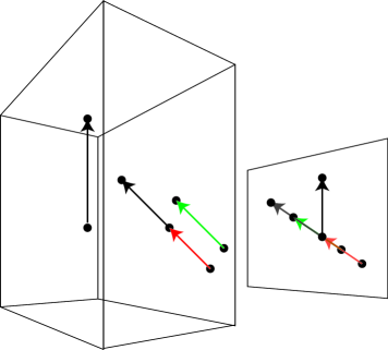
Figure 2: The projection from left to right defines a morphism from a configuration of $7$ points, $3$ lines, and $4$ segments in three dimensions to a configuration of $6$ points, $2$ lines, and $4$ segments in two dimensions.

Proposition 4.9.

Given $\mathbb{K}$, $\mathbf{p}$, $r$, $\ell$, the $D=r-1,\ldots,\infty$ union of the sets of $({\mathbf{p}},r,\ell,D)$-configurations, together with the above notion of morphism, forms a category.

Proof (sketch).

There is an identity morphism from any $\mathcal{S}$ to itself. It is straightforward to check that the usual composition of maps of sets $\mathcal{A}:\mathcal{P}(\mathcal{S})\to\mathcal{P}(\mathcal{T})$ and ${\mathbf{A}}:\mathcal{U}(\mathcal{S})\to\mathcal{U}(\mathcal{T})$ defines an associative composition of morphisms. ∎

Example 4.10.

The classical notion of projective equivalence is an important special case of morphism, as follows. Let $D^{\prime}=D$, and let ${\mathbf{A}}$ be an invertible $\mathbb{K}$-linear map $\mathbb{K}^{D+1}\to\mathbb{K}^{D+1}$. The induced map $A:\mathbb{K}P^{D}\to\mathbb{K}P^{D}$ is a projective transformation and a configuration $\mathcal{S}$ is projectively equivalent to its image $A(\mathcal{S})$. The restriction of $A$ to $\mathcal{P}(\mathcal{S})$ is a morphism $\mathcal{A}$ from $\mathcal{S}$ to $A(\mathcal{S})$ as in Definition 4.8. First, for any ordered representative of $\mathcal{S}_{c}$, $c=0,\ldots,n$, index the $r$-tuples in $A(\mathcal{S}_{c})=\mathcal{T}_{c}$ by setting $\vec{t}_{c}^{\ K}=A(\vec{s}_{c}^{K})$. The map ${\mathbf{A}}:\mathcal{U}(\mathcal{S})\to\mathbb{K}^{D+1}$ from the Definition is just the restriction of the given linear map to $\mathcal{U}(\mathcal{S})$, and restricts further to ${\mathbf{L}}=\pi^{-1}(L)$ for $L\in\mathcal{L}(\mathcal{S})$, so $\left.{\mathbf{A}}\right|_{\mathbf{L}}$ is one-to-one and linear, satisfying (1) and (2), so it induces $A_{L}:L\to\mathbb{K}P^{D}$. For each independent $r$-tuple $\vec{s}_{c}^{K}$ with span $L$, the induced map $A_{L}$ takes $\vec{s}_{c}^{K}$ to an independent $r$-tuple $A_{L}(\vec{s}_{c}^{K})=\vec{t}_{c}^{\ K}$.

Example 4.11.

In Example 4.10, checking Definition 4.8 did not require that $D^{\prime}=D$, nor that $\mathbf{A}$ was invertible. The same argument applies to any $\mathbb{K}$-linear $\mathbf{A}:\mathbb{K}^{D+1}\to\mathbb{K}^{D^{\prime}+1}$, which is not necessarily one-to-one or onto, but which is one-to-one when restricted to subspaces ${\mathbf{L}}=\pi^{-1}(L)$ for $L\in\mathcal{L}(\mathcal{S})$. As shown in Figure 2, the induced map $A$ could be a projection from a subset of a higher-dimensional projective space to a lower-dimensional space, and would define a morphism $\mathcal{A}$ from a configuration $\mathcal{S}$ to $A(\mathcal{S})$ as long as the image of every $(r-1)$-dimensional projective subspace in $\mathcal{L}(\mathcal{S})$ is still $(r-1)$-dimensional.

Definition 4.12.

A $({\mathbf{p}},r,\ell,D)$-configuration $\mathcal{S}$ is a weight $\mathbf{p}$ h-configuration means:

1. At every point $z\in\mathbb{K}P^{D}$, these numbers are integers and are equal to each other:

   $$\frac{deg_{0}(z)}{p_{0}}=\cdots=\frac{deg_{c}(z)}{p_{c}}=\cdots=\frac{deg_{n}(z)}{p_{n}};$$ (22)

2. For every projective $(r-1)$-subspace $L\subseteq\mathbb{K}P^{D}$, these numbers are integers and are equal to each other:

   $$\frac{deg_{0}(L)}{p_{0}}=\cdots=\frac{deg_{c}(L)}{p_{c}}=\cdots=\frac{deg_{n}(L)}{p_{n}}.$$ (23)

For a weight $\mathbf{p}$ h-configuration $\mathcal{S}$, we have the following geometric interpretation of the parameter $\ell$: if a $(r-1)$-dimensional projective subspace $L$ in $\mathcal{L}(\mathcal{S})$ has $deg_{c}(L)=m_{L}p_{c}$, then by (23), $m_{L}$ does not depend on $c$. There is an unordered $\ell$-tuple of subspaces, $[L_{1},\ldots,L_{k},\ldots,L_{\ell}]$, where each $L_{k}$ is incident with exactly $p_{c}$ $r$-tuples with color $c$, and $L_{k}$ occurs in the unordered list with multiplicity $m_{L_{k}}$.

Lemma 4.13.

If $\mathcal{S}$ is a weight $\mathbf{p}$ h-configuration and $\mathcal{A}:\mathcal{S}\to\mathcal{T}$ is a morphism, then $\mathcal{T}$ is a weight $\mathbf{p}$ h-configuration.

Proof.

Let the ordered $\ell p_{c}$-tuple $S_{c}$ be an ordered representative for $\mathcal{S}_{c}$; then let $T_{c}$ be the corresponding ordered representative of $\mathcal{T}_{c}$ as in (20). The $r$ points in $\vec{t}_{c}^{\ K}$ are indexed, using (2),

$$t_{c}^{K,e}=\mathcal{A}(s_{c}^{K,e}),$$ (24)

for $K=1,\ldots,\ell p_{c}$ and $e=1,\ldots,r$.

To check part 1. of Definition 4.12, suppose $z\in\mathbb{K}P^{D^{\prime}}$. If $z\notin\mathcal{P}(\mathcal{T})$, then $deg_{c}(z)=0$ for all $c$. If $z\in\mathcal{P}(\mathcal{T})$, then $\mathcal{A}^{-1}(z)$ is a finite set of points in $\mathcal{P}(\mathcal{S})$. There is no $r$-tuple $\vec{s}_{c}^{K}$ that contains more than one point of $\mathcal{A}^{-1}(z)$, since $\mathcal{A}(\vec{s}_{c}^{K})$ is the independent $r$-tuple $\vec{t}_{c}^{\ K}$. An $r$-tuple $\vec{t}_{c}^{\ K}$ has $z$ as one of its $r$ points if and only if the corresponding $r$-tuple $\vec{s}_{c}^{K}$ has some element of $\mathcal{A}^{-1}(z)$ as one of its $r$ points. For each $c$, the cardinality of the disjoint union of indices $K$ is:

$$deg_{c}(z)=\sum_{w\in\mathcal{A}^{-1}(z)}deg_{c}(w).$$

The equalities in (22) for $z$ follow from the assumed equalities for all the points $w$.

Dually, projective $(r-1)$-subspaces not in $\mathcal{L}(\mathcal{T})$ have $deg_{c}=0$ for all $c$. By (2), every projective $(r-1)$-subspace in $\mathcal{L}(\mathcal{T})$ is of the form $A_{L^{\prime}}(L^{\prime})$, and if $L^{\prime}$ is the span of $\vec{s}_{c}^{K^{\prime}}$, then all $r$ points $t_{c}^{K^{\prime},e}$ lie on $A_{L^{\prime}}(L^{\prime})$. The set $\mathcal{L}^{\prime}=\{L\in\mathcal{L}(\mathcal{S}):A_{L}(L)=A_{L^{\prime}}(L^{\prime})\}$ is finite, and there is no $r$-tuple $\vec{s}_{c}^{K}$ lying on more than one of these subspaces $L$. An $r$-tuple $\vec{t}_{c}^{\ K}$ lies on $A_{L^{\prime}}(L^{\prime})$ if and only if the corresponding $r$-tuple $\vec{s}_{c}^{K}$ lies on one of the subspaces $L\in\mathcal{L}^{\prime}$. For each $c$, the cardinality of the disjoint union of indices $K$ is:

$$deg_{c}(A_{L^{\prime}}(L^{\prime}))=\sum_{L\in\mathcal{L}^{\prime}}deg_{c}(L).$$

The equalities in (23) for $A_{L^{\prime}}(L^{\prime})$ follow from the assumed equalities for all $L\in\mathcal{L}^{\prime}$. ∎

4.2 The Invariant

Notation 4.14.

Given an $(r-1)$-dimensional projective subspace $L$ in $\mathbb{K}P^{D}$, which is the image of a $r$-dimensional subspace ${\mathbf{L}}$ in $\mathbb{K}^{D+1}$, $L=\pi({\mathbf{L}})$, let $\mathcal{B}=({\mathbf{b}_{0}},\ldots,{\mathbf{b}_{r-1}})$ be an ordered basis for ${\mathbf{L}}$. Given an independent set of vectors ${\mathbf{s}_{e}}\in{\mathbf{L}}$, $e=1,\ldots,r$, with $\pi({\mathbf{s}_{e}})=s_{e}$ on $L$, let $\vec{s}$ be the ordered $r$-tuple $(s_{1},\ldots,s_{r})$, and define $\llbracket\vec{s}\ \rrbracket_{\mathcal{B}}\in\mathbb{K}^{1}_{*}$ by the following procedure. The vectors have coordinates in the $\mathcal{B}$ basis:

$${\mathbf{s}_{e}}=s_{e}^{0}{\mathbf{b}_{0}}+\ldots+s_{e}^{r-1}{\mathbf{b}_{r-1}}\implies[{\mathbf{s}_{e}}]_{\mathcal{B}}=\left[\begin{array}[]{c}s_{e}^{0}\\ \vdots\\ s_{e}^{r-1}\end{array}\right]_{\mathcal{B}}\in\mathbb{K}^{r}.$$ (25)

By stacking columns into a square matrix, denote

$$\llbracket\vec{s}\ \rrbracket_{\mathcal{B}}=\det\left(\left[[{\mathbf{s}_{1}}]_{\mathcal{B}}\cdots[{\mathbf{s}_{e}}]_{\mathcal{B}}\cdots[{\mathbf{s}_{r}}]_{\mathcal{B}}\right]_{r\times r}\right).$$ (26)

For example, in the $r=2$ case,

$$\llbracket\vec{s}\ \rrbracket_{\mathcal{B}}=s_{2}^{1}s_{1}^{0}-s_{2}^{0}s_{1}^{1}.$$ (27)

The $r$-dimensional vector space ${\mathbf{L}}$, together with the extra structure in the RHS of (26), is called a Peano space by [BBR]. The Peano bracket of $\vec{s}$ as we have defined it in (26) depends on the choices of basis and representative points, and also on the ordering of points in $\vec{s}$. Note that picking a different representative $\lambda\cdot{\mathbf{s}_{e}}$ for the point $s_{e}$ and $\lambda\neq 0$ transforms $\llbracket\vec{s}\ \rrbracket_{\mathcal{B}}$ to $\lambda\cdot\llbracket\vec{s}\rrbracket_{\mathcal{B}}$.

Theorem 4.15.

Let $\mathcal{S}$ be a $({\mathbf{p}},r,\ell,D)$-configuration which is a weight $\mathbf{p}$ h-configuration. For each $c=0,\ldots,n$, choose an ordered representative $S_{c}$ of $\mathcal{S}_{c}$ as in (18). For each point $z$ in the set of points $\mathcal{P}(\mathcal{S})=\{s_{c}^{K,e}\}$, choose one representative vector ${\mathbf{z}}={\mathbf{s}}_{c}^{K,e}$. For each projective $(r-1)$-subspace $L$ in the set $\mathcal{L}(\mathcal{S})$, choose one ordered basis $\mathcal{B}_{L}$ for the $r$-subspace ${\mathbf{L}}=\pi^{-1}(L)$, and if the span of $\vec{s}_{c}^{K}$ is $L$, denote $\mathcal{B}_{c,K}=\mathcal{B}_{L}$. Then the following element of $\mathbb{K}P({\mathbf{p}})$ is well-defined, depending only on $\mathcal{S}$ and $\mathbf{p}$, and not the above choices.

$$E_{\mathbf{p}}(\mathcal{S})=\left[\prod_{K=1}^{\ell p_{0}}\llbracket\vec{s}_{0}^{K}\rrbracket_{\mathcal{B}_{0,K}}:\ldots:\prod_{K=1}^{\ell p_{c}}\llbracket\vec{s}_{c}^{K}\rrbracket_{\mathcal{B}_{c,K}}:\ldots:\prod_{K=1}^{\ell p_{n}}\llbracket\vec{s}_{n}^{K}\rrbracket_{\mathcal{B}_{n,K}}\right]_{\mathbf{p}}.$$

Further, if $\mathcal{T}$ is a $({\mathbf{p}},r,\ell,D^{\prime})$-configuration and $\mathcal{A}:\mathcal{S}\to\mathcal{T}$ is a morphism, then $E_{\mathbf{p}}(\mathcal{S})=E_{\mathbf{p}}(\mathcal{T})$.

Proof.

The choice of ordering $S_{c}$ as in (18) is used only for well-defined indexing; the first thing to prove is that the $E_{\mathbf{p}}$ expression does not depend on this choice. The second part of the Proof is to show the expression does not depend on the choices made in computing the bracket (26). The third part of the Proof is verifying the invariance under morphism.

First, for each ordered $r$-tuple $\vec{s}_{c}^{K}$ in $S_{c}$, formula (26) shows that the quantity $\llbracket\vec{s}_{c}^{K}\rrbracket_{\mathcal{B}_{c,K}}\in\mathbb{K}^{1}_{*}$ depends on a choice of basis $\mathcal{B}_{c,K}$ and a choice of representative vectors for the $r$ points. By the independence property, the $r$ points of each $\vec{s}_{c}^{K}$ span a unique projective $(r-1)$-subspace $L$, for which a unique basis $\mathcal{B}_{L}$ was chosen, by hypothesis. So, the basis used to compute $\llbracket\vec{s}_{c}^{K}\rrbracket_{\mathcal{B}_{c,K}}$ depends only on the $r$ points of $\vec{s}_{c}^{K}$ in $\mathbb{K}P^{D}$. Each of the points $s_{c}^{K,e}$ has a representative in $\mathbb{K}^{D+1}_{*}$ that does not depend on the color index $c$ or the assignment of $K$ index to the $r$-tuple $\vec{s}_{c}^{K}$. The construction as stated in the hypothesis requires picking the same representative vector $\mathbf{z}$ when a point appears more than once in the $\mathcal{S}$ configuration, in $r$-tuples with different indices or colors: if $z=s_{c}^{K,e}=s_{c^{\prime}}^{K^{\prime},e^{\prime}}$ then ${\mathbf{z}}={\mathbf{s}}_{c}^{K,e}={\mathbf{s}}_{c^{\prime}}^{K^{\prime},e^{\prime}}$. We can conclude that $\llbracket\vec{s}_{c}^{K}\rrbracket_{\mathcal{B}_{c,K}}$ is computed using representative vectors of the points and a basis, both depending only on the $r$-tuple of points and not on the index $K$ coming from $S_{c}$. By commutativity, the product $\displaystyle{\prod_{K=1}^{\ell\cdot p_{c}}\llbracket\vec{s}_{c}^{K}\rrbracket_{\mathcal{B}_{c,K}}}$ does not depend on the choice of ordered representative $S_{c}$ for $\mathcal{S}_{c}$, nor on ${\mathbf{p}}$, since $\ell\cdot p_{c}$ is uniquely determined by $\mathcal{S}$. The element

$$\left[\prod_{K=1}^{\ell p_{0}}\llbracket\vec{s}_{0}^{K}\rrbracket_{\mathcal{B}_{0,K}}:\ldots:\prod_{K=1}^{\ell p_{n}}\llbracket\vec{s}_{n}^{K}\rrbracket_{\mathcal{B}_{n,K}}\right]_{\mathbf{p}}\in\mathbb{K}P({\mathbf{p}})$$

may depend on ${\mathbf{p}}$, as in Theorem 2.12. We can conclude so far that the above expression depends only on $\mathcal{S}$ and $\mathbf{p}$, not on any of the choices of $S_{c}$.

The independence property implies the quantities $\llbracket\vec{s}_{c}^{K}\rrbracket_{\mathcal{B}_{c,K}}$ are all non-zero, so each of the $n+1$ components in the $E_{\mathbf{p}}$ expression is non-zero: $E_{\mathbf{p}}(\mathcal{S})\in D_{\mathbf{p}}$.

For the second part of the Proof, as previously mentioned, for each point $z$ occurring with any multiplicity in the $\mathcal{S}$ configuration, the construction of the Theorem requires choosing a fixed representative $\mathbf{z}$. Changing the choice of representative for that point, $\lambda\cdot{\mathbf{z}}$ instead of $\mathbf{z}$, changes each $\llbracket\vec{s}_{c}^{K}\rrbracket_{\mathcal{B}_{c,K}}$ quantity to $\lambda\cdot\llbracket\vec{s}_{c}^{K}\rrbracket_{\mathcal{B}_{c,K}}$, as remarked after Notation 4.14, for every $\vec{s}_{c}^{K}$ that has $z$ as one of its $r$ points (and only one, by independence). In each expression $\displaystyle{\prod_{K=1}^{\ell\cdot p_{c}}\llbracket\vec{s}_{c}^{K}\rrbracket_{\mathcal{B}_{c,K}}}$ (with color index $c$), there are $deg_{c}(z)$ (possibly repeated) $r$-tuples $\vec{s}_{c}^{K}$ with $z$ as one of its $r$ points, so changing ${\mathbf{z}}$ to $\lambda\cdot{\mathbf{z}}$ changes the product expression by a factor of $\lambda^{deg_{c}(z)}$. By part 1. of Definition 4.12, there is some integer $y$ depending on $z$ but not $c$, so that $deg_{c}(z)=y\cdot p_{c}$. Since for each $c$, the product changes by a factor of $(\lambda^{y})^{p_{c}}$, the $\sim_{\mathbf{p}}$-equivalence class of the $E_{\mathbf{p}}$ expression does not depend on the choice of $\lambda$ or ${\mathbf{z}}$.

For a projective $(r-1)$-subspace $L$, the value of the bracket $\llbracket\vec{s}_{c}^{K}\rrbracket_{\mathcal{B}_{c,K}}$ depends on the choice of ordered basis $\mathcal{B}_{c,K}=\mathcal{B}_{L}=\left({\mathbf{b}}_{0},\ldots,{\mathbf{b}}_{r-1}\right)$ in the following way: let $\mathcal{B}_{L}^{\prime}$ be another ordered basis of the same $r$-dimensional space ${\mathbf{L}}$. Then there exists a $r\times r$ invertible matrix $Q$ which changes $\mathcal{B}_{L}$-coordinates to $\mathcal{B}_{L}^{\prime}$-coordinates, via matrix multiplication: if the $\mathcal{B}_{L}$-coordinate column vector of ${\mathbf{s}}_{c}^{K,e}$ is as in (25), then the $\mathcal{B}_{L}^{\prime}$-coordinate column vector is $[{\mathbf{s}}_{c}^{K,e}]_{\mathcal{B}_{L}^{\prime}}=Q[{\mathbf{s}}_{c}^{K,e}]_{\mathcal{B}_{L}}$. Applying the $Q$ coordinate change matrix to each column in the determinant (26) transforms the bracket by the well-known formula

$$\llbracket\vec{s}_{c}^{K}\rrbracket_{\mathcal{B}_{L}^{\prime}} = \det\left(\left[(Q[{\mathbf{s}}_{c}^{K,1}]_{\mathcal{B}_{L}})\cdots(Q[{\mathbf{s}}_{c}^{K,r}]_{\mathcal{B}_{L}})\right]_{r\times r}\right)$$

$$= \det(Q)\det\left(\left[[{\mathbf{s}}_{c}^{K,1}]_{\mathcal{B}_{L}}\cdots[{\mathbf{s}}_{c}^{K,r}]_{\mathcal{B}_{L}}\right]_{r\times r}\right)$$

$$= \det(Q)\llbracket\vec{s}_{c}^{K}\rrbracket_{\mathcal{B}_{L}}.$$

We can conclude that for any $L$, changing the choice of ordered basis $\mathcal{B}_{L}$ to a new basis $\mathcal{B}_{L}^{\prime}$, and using this new basis for every bracket expression for an $r$-tuple on $L$, results in changing each expression with color index $c$, $\displaystyle{\prod_{K=1}^{\ell p_{c}}\llbracket\vec{s}_{c}^{K}\rrbracket_{\mathcal{B}_{c,K}}}$, by a factor of $(\det(Q))^{deg_{c}(L)}$, where $deg_{c}(L)=m_{L}p_{c}$, and $m_{L}$ does not depend on $c$, by part 2. of Definition 4.12. Since for each $c$, the product changes by a factor of $(\det(Q)^{m_{L}})^{p_{c}}$, the $\sim_{\mathbf{p}}$-equivalence class of $E_{\mathbf{p}}$ is unchanged. This shows that $E_{\mathbf{p}}$ does not depend on the choices made as in the statement of the Theorem, which are required to compute the brackets $\llbracket\vec{s}_{c}^{K}\rrbracket_{\mathcal{B}_{L}}$.

Thirdly, by Lemma 4.13, if there is a morphism $\mathcal{A}:\mathcal{S}\to\mathcal{T}$, then $\mathcal{T}$ is also a weight $\mathbf{p}$ h-configuration, and so the expression $E_{\mathbf{p}}(\mathcal{T})$ is well-defined by the previous part of this Proof. As in the Proof of Lemma 4.13, an ordering for $\mathcal{S}_{c}$ corresponds to one for $\mathcal{T}_{c}$, giving an indexing as in (24).

For each projective $(r-1)$-subspace $A_{L}(L)$ in the set $\mathcal{L}(\mathcal{T})$, pick an ordered basis $\mathcal{C}$ for the linear $r$-subspace ${\mathbf{A}}|_{{\mathbf{L}}}({\mathbf{L}})$, as in the hypothesis of the Theorem applied to $\mathcal{L}(\mathcal{T})$. For any ${\mathbf{L}}^{\prime}$ with $A_{L^{\prime}}(L^{\prime})=A_{L}(L)$, ${\mathbf{A}}|_{{\mathbf{L}}^{\prime}}$ is linear and one-to-one, so $\left({\mathbf{A}}|_{{\mathbf{L}}^{\prime}}\right)^{-1}(\mathcal{C})$ is an ordered basis for ${\mathbf{L}}^{\prime}$, and setting $\mathcal{B}_{L^{\prime}}=\left({\mathbf{A}}|_{{\mathbf{L}}^{\prime}}\right)^{-1}(\mathcal{C})$ satisfies the uniqueness hypothesis of the Theorem applied to $\mathcal{L}(\mathcal{S})$.

Dually, for each point $w=t_{c}^{K,e}$ in the set $\mathcal{P}(\mathcal{T})$, pick a representative ${\mathbf{w}}={\mathbf{t}}_{c}^{K,e}$ in $\mathbb{K}^{D^{\prime}+1}_{*}$ as in the hypothesis. For an index $(c,K,e)$, the point $s_{c}^{K,e}$ lies on a $(r-1)$-subspace $L_{c,K}$ spanned by $\vec{s}_{c}^{K}$, and satisfies $A_{L_{c,K}}(s_{c}^{K,e})=t_{c}^{K,e}$, and has a representative vector $({\mathbf{A}}|_{{\mathbf{L}_{c,K}}})^{-1}({\mathbf{t}}_{c}^{K,e})$ in $\mathbb{K}^{D+1}_{*}$. To show that this representative vector depends only on the point and not on the index, suppose $(c^{\prime},K^{\prime},e^{\prime})$ is any other index with $s_{c}^{K,e}=s_{c^{\prime}}^{K^{\prime},e^{\prime}}$; then the point is on both projective $(r-1)$-subspaces $L_{c,K}$ and $L_{c^{\prime},K^{\prime}}$, and ${\mathbf{A}}|_{{\mathbf{L}}_{c,K}}$ and ${\mathbf{A}}|_{{\mathbf{L}}_{c^{\prime},K^{\prime}}}$ agree on the intersection ${\mathbf{L}}_{c,K}\cap{\mathbf{L}}_{c^{\prime},K^{\prime}}$ because they are restrictions of the same map $\mathbf{A}$. Since ${\mathbf{t}}_{c}^{K,e}={\mathbf{t}}_{c^{\prime}}^{K^{\prime},e^{\prime}}$, we can conclude $({\mathbf{A}}|_{{\mathbf{L}}_{c,K}})^{-1}({\mathbf{t}}_{c}^{K,e})=({\mathbf{A}}|_{{\mathbf{L}}_{c^{\prime},K^{\prime}}})^{-1}({\mathbf{t}}_{c^{\prime}}^{K^{\prime},e^{\prime}})$, and denote this representative vector ${\mathbf{s}}_{c}^{K,e}$.

Now, fix an index pair $(c,K)$ and consider corresponding $r$-tuples $\vec{s}_{c}^{K}$ and $\vec{t}_{c}^{\ K}$, lying on subspaces $L_{c,K}$ and $A_{L_{c,K}}(L_{c,K})$ as above. The coordinate vector of ${\mathbf{t}}_{c}^{K,e}$ with respect to the ordered basis $\mathcal{C}=\left({\mathbf{c}}_{0},\ldots,{\mathbf{c}}_{r-1}\right)$ of ${\mathbf{A}}|_{{\mathbf{L}_{c,K}}}({\mathbf{L}}_{c,K})$ is related to the coordinate vector of ${\mathbf{s}}_{c}^{K,e}$ with respect to the ordered basis $\mathcal{B}_{c,K}=\left({\mathbf{A}}|_{{\mathbf{L}_{c,K}}}\right)^{-1}(\mathcal{C})$ of ${\mathbf{L}}_{c,K}$, by the linearity of ${\mathbf{A}}|_{{\mathbf{L}}_{c,K}}$:

$$({\mathbf{s}}_{c}^{K,e}) = \left({\mathbf{A}}|_{{\mathbf{L}}_{c,K}}\right)^{-1}({\mathbf{t}}_{c}^{K,e})$$

$$= \left({\mathbf{A}}|_{{\mathbf{L}}_{c,K}}\right)^{-1}(t_{c}^{K,e,0}{\mathbf{c}}_{0}+\ldots+t_{c}^{K,e,r-1}{\mathbf{c}}_{r-1})$$

$$= t_{c}^{K,e,0}\left({\mathbf{A}}|_{{\mathbf{L}}_{c,K}}\right)^{-1}({\mathbf{c}}_{0})+\ldots+t_{c}^{K,e,r-1}\left({\mathbf{A}}|_{{\mathbf{L}}_{c,K}}\right)^{-1}({\mathbf{c}}_{r-1})$$

$$= t_{c}^{K,e,0}{\mathbf{b}}_{c,K,0}+\ldots+t_{c}^{K,e,r-1}{\mathbf{b}}_{c,K,r-1},$$

i.e., the $\mathcal{B}_{c,K}$-coordinates of ${\mathbf{s}}_{c}^{K,e}$ are the same as the $\mathcal{C}$-coordinates of ${\mathbf{t}}_{c}^{K,e}$, and

$$\llbracket\vec{s}_{c}^{K}\rrbracket_{\mathcal{B}_{c,K}} = \det\left(\left[[{\mathbf{s}}_{c}^{K,1}]_{\mathcal{B}_{c,K}}\cdots[{\mathbf{s}}_{c}^{K,r}]_{\mathcal{B}_{c,K}}\right]_{r\times r}\right)$$

$$= \det\left(\left[[{\mathbf{t}}_{c}^{K,1}]_{\mathcal{C}}\cdots[{\mathbf{t}}_{c}^{K,r}]_{\mathcal{C}}\right]_{r\times r}\right)$$

$$= \llbracket\vec{t}_{c}^{\ K}\rrbracket_{\mathcal{C}}.$$

Using these brackets to compute the products in the $E_{\mathbf{p}}(\mathcal{S})$ expression, and the previously established fact that $E_{\mathbf{p}}(\mathcal{S})$ does not depend on the indexing $S_{c}$, or the choices of $\mathcal{B}_{L}$ or representative vectors, the claimed equality $E_{\mathbf{p}}(\mathcal{S})=E_{\mathbf{p}}(\mathcal{T})$ is proved. ∎

Example 4.16.

For ${\mathbf{p}}=(1,1)$, $n=1$ and there are two colors. $E_{(1,1)}(\mathcal{S})$ is a ratio of products of $\ell$ determinants of size $r\times r$, which, as stated in the Introduction, would have been recognizable before Eves’ time. The case ${\mathbf{p}}=(1,1)$, $r=2$, of Theorem 4.15 can be called a purely projective, or algebraic, version of Eves’ Theorem, in comparison to the Euclidean, or metric, version, Theorem 6.2.2 of [E]. The connection between the determinantal expression and Eves’ formula involving Euclidean signed lengths in $\mathbb{R}^{D}$ is discussed in Section 5.

For $r=2$, in a $((1,1),2,\ell,D)$-configuration $\mathcal{S}$, $\mathcal{S}_{0}$ is a list of $\ell$ black directed segments in $\mathbb{K}P^{D}$, and $\mathcal{S}_{1}$ is a list of $\ell$ red segments. If $\mathcal{S}$ is a weight $\mathbf{p}$ h-configuration (which in this ${\mathbf{p}}=(1,1)$, $r=2$ case we just call an h-configuration), then there are $\ell$ (counting with multiplicity) lines $[L_{1},\ldots,L_{\ell}]$ with one black segment $\vec{s}_{0}^{K}$ and one red segment $\vec{s}_{1}^{K}$ on each line, and at each point, the black degree equals the red degree. The following element of $\mathbb{K}P^{1}$, where each expression $\llbracket\vec{s}_{c}^{K}\rrbracket_{\mathcal{B}_{c,K}}$ is calculated as in Theorem 4.15, is well-defined and invariant under projective transformations of $\mathbb{K}P^{D}$:

$$E_{(1,1)}(\mathcal{S})=\left[\prod_{K=1}^{\ell}\llbracket\vec{s}_{0}^{K}\rrbracket_{\mathcal{B}_{0,K}}:\prod_{K=1}^{\ell}\llbracket\vec{s}_{1}^{K}\rrbracket_{\mathcal{B}_{1,K}}\right].$$

Eves calls the ratio

$$\frac{\displaystyle{\prod_{K=1}^{\ell}\llbracket\vec{s}_{1}^{K}\rrbracket_{\mathcal{B}_{1,K}}}}{\displaystyle{\prod_{K=1}^{\ell}\llbracket\vec{s}_{0}^{K}\rrbracket_{\mathcal{B}_{0,K}}}}$$

an “h-expression”: each line $L_{K}$ occurs equally often (multiplicity $m_{L_{K}}$) in the numerator and denominator, and each point in $\mathcal{P}(\mathcal{S})$ occurs equally often in the numerator (red degree) and denominator (black degree).

Example 4.17.

Consider four distinct points $\alpha$, $\beta$, $\gamma$, $\delta$ on the projective line $\mathbb{K}P^{1}$. These can be organized into an h-configuration $\mathcal{S}$, with ${\mathbf{p}}=(1,1)$ and $r=2$ as in Example 4.16, dimension $D=1$, and $\ell=2$. Let $\mathcal{S}_{0}=[(\delta,\alpha),(\gamma,\beta)]$ be a list of black segments, and let $\mathcal{S}_{1}=[(\gamma,\alpha),(\delta,\beta)]$ be a list of red segments, as shown in Figure 3. Then $\mathcal{L}(\mathcal{S})$ is the singleton set $\{L=\mathbb{K}P^{1}\}$; we could, as mentioned after Definition 4.12, consider the line occurring with multiplicity two in the unordered list $[L_{1},L_{2}]$ with $L=L_{1}=L_{2}$. Choose the standard ordered basis $\mathcal{B}_{L}=\left((1,0),(0,1)\right)$ of $\mathbb{K}^{2}$, so $\alpha$ has homogeneous coordinates $[\alpha_{0}:\alpha_{1}]$, vector representative $\alpha_{0}{\mathbf{b}}_{0}+\alpha_{1}{\mathbf{b}}_{1}$, and $\mathcal{B}_{L}$-coordinate vector $\left[\begin{array}[]{c}\alpha_{0}\\ \alpha_{1}\end{array}\right]$, and similarly for the other points. Let $S_{0}=(\vec{s}_{0}^{1}=(\delta,\alpha),\vec{s}_{0}^{\ 2}=(\gamma,\beta))$ be an ordered representative of $\mathcal{S}_{0}$ and let $S_{1}=(\vec{s}_{1}^{1}=(\gamma,\alpha),\vec{s}_{1}^{\ 2}=(\delta,\beta))$ be an ordered representative of $\mathcal{S}_{1}$. Each endpoint has black degree and red degree both equal to $1$, and the line $L$ satisfies Part 2. of Definition 4.12, with $deg_{0}(L)=deg_{1}(L)=2$. Alternatively, we could assign one of the black segments and one of the red segments to $L_{1}=L$, and the remaining segments to $L_{2}=L$; there are various choices of such assignments, which would not affect the expression (4.17). The expression from Theorem 4.15 is:

$$E_{(1,1)}(\mathcal{S}) = \left[\llbracket\vec{s}_{0}^{1}\rrbracket_{\mathcal{B}_{L}}\llbracket\vec{s}_{0}^{\ 2}\rrbracket_{\mathcal{B}_{L}}:\llbracket\vec{s}_{1}^{1}\rrbracket_{\mathcal{B}_{L}}\llbracket\vec{s}_{1}^{\ 2}\rrbracket_{\mathcal{B}_{L}}\right]$$

$$= \left[(\alpha_{1}\delta_{0}-\alpha_{0}\delta_{1})(\beta_{1}\gamma_{0}-\beta_{0}\gamma_{1}):(\alpha_{1}\gamma_{0}-\alpha_{0}\gamma_{1})(\beta_{1}\delta_{0}-\beta_{0}\delta_{1})\right],$$

which is exactly the well-known cross-ratio of the ordered quadruple $(\alpha,\beta,\gamma,\delta)$.

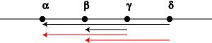
Figure 3: A configuration of $4$ points, $1$ line, and $4$ ordered pairs, as indicated by the red and black arrows drawn offset from the line.

In classical Invariant Theory, the fundamental property of projective invariance of the cross-ratio was often proved using determinants and algebraic methods similar to our Proof of Theorem 4.15 (e.g., [C]; [Salmon] Arts. XIII.136, 137, XVII.195). In projective geometry, the general idea that projective transformations introduce canceling factors in certain product expressions already appears in ([P] §20).

5 Metric versions

Eves’ Theorem as stated in [E] is about ratios of signed lengths of directed segments, in the real Euclidean plane extended to include points at infinity. The earlier identities of [P], and interesting applications of Eves’ Theorem, including Ceva’s Theorem and others appearing in ([E] §6.2), [F₂], and [Shephard], also involve Euclidean distance between pairs of points. The constructions in Section 4 were developed in terms of linear algebra and projective geometry, avoiding any notion of distance. However, there are connections between projective geometry and Euclidean geometry — a thorough, modern treatment is given by [RG], relating Cartesian coordinates in affine neighborhoods and bracket operations (as in the above Notation 4.14) to distance, area, volume, angles, etc.

For this Section, we consider only the case $\mathbb{K}=\mathbb{R}$, and start by incorporating a notion of distance, as a bit of extra structure added to the projective coordinate system.

Consider, as in Example 2.3, $\mathbb{R}^{D+1}$ with coordinates ${\mathbf{x}}=(x_{0},x_{1},\ldots,x_{D})$, the projection $\pi:\mathbb{R}^{D+1}_{*}\to\mathbb{R}P^{D}$, and homogeneous coordinates $x=[x_{0}:x_{1}:\ldots:x_{D}]$ for $\mathbb{R}P^{D}$. The restriction of $\pi$ to the hyperplane $\{(1,x_{1},x_{2},\ldots,x_{D})\}$ is one-to-one onto the image $\{x:x_{0}\neq 0\}$ in $\mathbb{R}P^{D}$. We can refer to this affine neighborhood as $\mathbb{R}^{D}$, where a point in $\mathbb{R}^{D}$ has both homogeneous and affine coordinates: $x=[1:x_{1}:\ldots:x_{D}]=(x_{1},\ldots,x_{D})$, and also is the image of a representative vector: $x=\pi({\mathbf{x}})=\pi(1,x_{1},\ldots,x_{D})$.

The extra structure we choose to assign to the affine neighborhood $\mathbb{R}^{D}$ is that of a normed vector space, where the vector space structure is the usual one from the affine coordinate system $(x_{1},\ldots,x_{D})$, and $\|\ .\ \|$ is any norm function. Then there is a distance function on $\mathbb{R}^{D}$: ${\mathbf{d}}(x,y)=\|y-x\|$.

In the $r=2$ case, we are interested in directed segments on lines. Given a line $L$ in $\mathbb{R}^{D}$ (meaning, a non-empty intersection of a projective line $L=\pi({\mathbf{L}})$ with the $\{x:x_{0}\neq 0\}$ neighborhood), it can be parametrized by choosing a start point $b_{0}$ and a non-zero direction vector $v$, so $L=\{b_{0}+tv:t\in\mathbb{R}\}$. The choice of $v$ also determines a direction for the line: an ordered pair of distinct points $(b_{0}+t_{1}v,b_{0}+t_{2}v)$ is a positively (or negatively) directed segment depending on the sign of $t_{2}-t_{1}$. There exists a unique $t$ value so that $t>0$ and the point $b_{1}=b_{0}+tv$ satisfies ${\mathbf{d}}(b_{0},b_{1})=1$. Choose these representative vectors in $\mathbb{R}^{D+1}$ for $b_{0}$ and $b_{1}$: ${\mathbf{b}_{0}}=(1,b_{0}^{1},\ldots,b_{0}^{D})$ and ${\mathbf{b}_{1}}=(1,b_{1}^{1},\ldots,b_{1}^{D})$. So, choosing a start point and a direction for the affine line $L$ determines (and is determined by) an ordered basis $\mathcal{B}=({\mathbf{b}_{0}},{\mathbf{b}_{1}})$ (with both points in $\{x_{0}=1\}$) for the plane ${\mathbf{L}}$.

Consider two distinct points $\alpha$, $\beta$ on the line $L$ in $\mathbb{R}^{D}\subseteq\mathbb{R}P^{D}$. If we re-parametrize $L$ using $b_{1}-b_{0}$ as a direction vector,

$$\alpha = (b_{0}^{1}+t_{1}(b_{1}^{1}-b_{0}^{1}),\ldots,b_{0}^{D}+t_{1}(b_{1}^{D}-b_{0}^{D})),$$

$$\beta = (b_{0}^{1}+t_{2}(b_{1}^{1}-b_{0}^{1}),\ldots,b_{0}^{D}+t_{2}(b_{1}^{D}-b_{0}^{D})).$$

The distance from $\alpha$ to $\beta$ does not depend on the choice of start point $b_{0}$ nor the direction; it satisfies:

$${\mathbf{d}}(\alpha,\beta) = \|\beta-\alpha\|=\|(t_{2}-t_{1})(b_{1}-b_{0})\|$$

$$= |t_{2}-t_{1}|\|b_{1}-b_{0}\|=|t_{2}-t_{1}|.$$

The signed length of the directed segment $(\alpha,\beta)=\overrightarrow{\alpha\beta}$ is $t_{2}-t_{1}$, which depends on the direction but not the start point. Choosing the representative vectors

$$\alpha = (1,b_{0}^{1}+t_{1}(b_{1}^{1}-b_{0}^{1}),\ldots,b_{0}^{D}+t_{1}(b_{1}^{D}-b_{0}^{D}))=(1-t_{1}){\mathbf{b}_{0}}+t_{1}{\mathbf{b}_{1}},$$ (29)

$$\beta = (1,b_{0}^{1}+t_{2}(b_{1}^{1}-b_{0}^{1}),\ldots,b_{0}^{D}+t_{2}(b_{1}^{D}-b_{0}^{D}))=(1-t_{2}){\mathbf{b}_{0}}+t_{2}{\mathbf{b}_{1}},$$

the signed length is exactly the same as the bracket formula (27):

$$\llbracket\overrightarrow{\alpha\beta}\rrbracket_{\mathcal{B}} = t_{2}(1-t_{1})-(1-t_{2})t_{1}=t_{2}-t_{1}.$$

When $\llbracket\overrightarrow{\alpha\beta}\rrbracket_{\mathcal{B}}$ expressions are used in Theorem 4.15, the expression $E_{\mathbf{p}}(\mathcal{S})$ does not depend on the choice of representative vectors $\alpha$, $\beta$ as long as representatives are chosen consistently (as in (29)), nor on the choice of $\mathcal{B}$ as long as that ordered basis is used for all directed segments on that line. Since the construction requires each line $L$ to be assigned a unique ordered basis $\mathcal{B}_{L}$, each line can have its own choice of direction determined by $\mathcal{B}_{L}$, and a unit of length depending on a norm $\|\ .\ \|_{L}$. So, a metric version for the $r=2$ (directed segments) case of Theorem 4.15 can be stated as follows.

Corollary 5.1.

Given a weight $\mathbf{p}$ h-configuration $\mathcal{S}$ of points in $\mathbb{R}^{D}$ with $r=2$, choose ordered representatives as in (18), and for each line $L$ in the set $\mathcal{L}(\mathcal{S})$, choose a direction and unit of length so that $\llbracket\overrightarrow{\alpha\beta}\rrbracket$ denotes the signed length of directed segments on the line through $\alpha$ and $\beta$. The following element of $\mathbb{R}P({\mathbf{p}})$ does not depend on the choices of ordered representatives, directions, or unit lengths.

$$E_{\mathbf{p}}(\mathcal{S})=\left[\prod_{K=1}^{\ell p_{0}}\llbracket\vec{s}_{0}^{K}\rrbracket:\ldots:\prod_{K=1}^{\ell p_{c}}\llbracket\vec{s}_{c}^{K}\rrbracket:\ldots:\prod_{K=1}^{\ell p_{n}}\llbracket\vec{s}_{n}^{K}\rrbracket\right]_{\mathbf{p}}.$$

Further, $E_{\mathbf{p}}(\mathcal{S})$ is invariant under a morphism that maps the points in $\mathcal{S}$ into an affine neighborhood $\mathbb{R}^{D^{\prime}}$.  

The Peano bracket also admits a Euclidean interpretation in the above coordinate system for configurations with $r=3$ and $D=2$ (see [BB], [CRG], in addition to the previously mentioned [RG]). However, in order for the bracket to define a Euclidean area in $\mathbb{R}^{2}$, we must use the Euclidean magnitude $\|\ .\ \|$, defined by the standard dot product in the affine coordinate system $(x_{1},x_{2})$. Let $L$ be the entire real projective plane $L=\mathbb{R}P^{2}$, and let ${\mathbf{L}}=\mathbb{R}^{3}$. Pick the standard ordered basis $\mathcal{B}$, so that three points $\alpha=(\alpha_{1},\alpha_{2})$, $\beta=(\beta_{1},\beta_{2})$, $\gamma=(\gamma_{1},\gamma_{2})$ in $\mathbb{R}^{2}\subseteq\mathbb{R}P^{2}$ have representatives with $\mathcal{B}$-coordinates ${\mbox{\boldmath$\alpha$}}=\left[\begin{array}[]{c}1\\ \alpha_{1}\\ \alpha_{2}\end{array}\right]_{\mathcal{B}}$, etc. Then,

$$\llbracket(\alpha,\beta,\gamma)\rrbracket_{\mathcal{B}}=\det\left(\left[\left[\begin{array}[]{c}1\\ \alpha_{1}\\ \alpha_{2}\end{array}\right]_{\mathcal{B}}\left[\begin{array}[]{c}1\\ \beta_{1}\\ \beta_{2}\end{array}\right]_{\mathcal{B}}\left[\begin{array}[]{c}1\\ \gamma_{1}\\ \gamma_{2}\end{array}\right]_{\mathcal{B}}\right]_{3\times 3}\right)=2Area\triangle(\alpha\beta\gamma),$$

twice the signed area of the triangle ([E] §2.1), which depends on the ordering of the three points and the (previously chosen) standard Euclidean structure on $\mathbb{R}^{2}$. The points with affine coordinates $(0,0)$, $(1,0)$, $(0,1)$, in that order, form a counter-clockwise triangle with positive area $\frac{1}{2}$.

The following Example of ratios of areas was described by [C] as a “graphometric” quantity: a Euclidean measurement invariant under projective transformations.

Example 5.2.

Consider six points, labeled ${\mathnormal{1}},{\mathnormal{2}},{\mathnormal{3}},{\mathnormal{4}},{\mathnormal{5}},{\mathnormal{6}}$, in the plane $\mathbb{R}^{2}\subseteq\mathbb{R}P^{2}$. They can be organized into a $((1,1),3,2,2)$-configuration $\mathcal{S}=(\mathcal{S}_{0},\mathcal{S}_{1})$, where

$$\mathcal{S}_{0}=[\triangle({\mathnormal{1}}{\mathnormal{2}}{\mathnormal{4}}),\triangle({\mathnormal{3}}{\mathnormal{5}}{\mathnormal{6}})]$$

is a list of two black triangles, and

$$\mathcal{S}_{1}=[\triangle({\mathnormal{1}}{\mathnormal{2}}{\mathnormal{3}}),\triangle({\mathnormal{4}}{\mathnormal{5}}{\mathnormal{6}})]$$

is a list of two red triangles (assuming non-collinearity of the indicated triples), as in Figure 4. Then $\mathcal{L}(\mathcal{S})=\{L=\mathbb{R}P^{2}\}$, and we choose the standard basis $\mathcal{B}$ as above. As in Example 4.17, $deg_{0}(L)=deg_{1}(L)=2$, or we could consider a list $[L_{1},L_{2}]$ with $L_{1}=L_{2}=L$, and one black triangle and one red triangle is assigned to each of $L_{1}$ and $L_{2}$. Each of the six points in $\mathcal{P}(\mathcal{S})$ is a vertex of one black triangle and one red triangle, so the black degree equals the red degree and $\mathcal{S}$ is a weight $(1,1)$ h-configuration. The invariant from Theorem 4.15 is analogous to (4.17):

$$E_{(1,1)}(\mathcal{S}) = \left[\llbracket\vec{s}_{0}^{1}\rrbracket_{\mathcal{B}}\llbracket\vec{s}_{0}^{\ 2}\rrbracket_{\mathcal{B}}:\llbracket\vec{s}_{1}^{1}\rrbracket_{\mathcal{B}}\llbracket\vec{s}_{1}^{\ 2}\rrbracket_{\mathcal{B}}\right]$$

$$= \left[\llbracket\triangle({\mathnormal{1}}{\mathnormal{2}}{\mathnormal{4}})\rrbracket_{\mathcal{B}}\llbracket\triangle({\mathnormal{3}}{\mathnormal{5}}{\mathnormal{6}})\rrbracket_{\mathcal{B}}:\llbracket\triangle({\mathnormal{1}}{\mathnormal{2}}{\mathnormal{3}})\rrbracket_{\mathcal{B}}\llbracket\triangle({\mathnormal{4}}{\mathnormal{5}}{\mathnormal{6}})\rrbracket_{\mathcal{B}}\right].$$

We can conclude that the ratio of signed areas

$$\frac{(Area\triangle({\mathnormal{1}}{\mathnormal{2}}{\mathnormal{3}}))(Area\triangle({\mathnormal{4}}{\mathnormal{5}}{\mathnormal{6}}))}{(Area\triangle({\mathnormal{1}}{\mathnormal{2}}{\mathnormal{4}}))(Area\triangle({\mathnormal{3}}{\mathnormal{5}}{\mathnormal{6}}))}$$

is an invariant of the configuration $\mathcal{S}$ under projective transformations (that do not send any of the six points to infinity).

We remark that the property $E_{(1,1)}(\mathcal{S}^{(0,1)})=[1:1]$, or equivalently $\llbracket\triangle({\mathnormal{1}}{\mathnormal{2}}{\mathnormal{4}})\rrbracket_{\mathcal{B}}\llbracket\triangle({\mathnormal{3}}{\mathnormal{5}}{\mathnormal{6}})\rrbracket_{\mathcal{B}}-\llbracket\triangle({\mathnormal{1}}{\mathnormal{2}}{\mathnormal{3}})\rrbracket_{\mathcal{B}}\llbracket\triangle({\mathnormal{4}}{\mathnormal{5}}{\mathnormal{6}})\rrbracket_{\mathcal{B}}=0$, admits a projective (not necessarily Euclidean) interpretation as the concurrence of the lines through $\{{\mathnormal{1}},{\mathnormal{2}}\}$, $\{{\mathnormal{3}},{\mathnormal{4}}\}$, $\{{\mathnormal{5}},{\mathnormal{6}}\}$ ([CRG], [RG] Ch. 6).

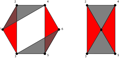
Figure 4: Left: A configuration of $6$ points and $4$ triangles in the real plane, from Example 5.2. Right: The points ${\mathnormal{1}}$ and ${\mathnormal{6}}$ coincide, as in Example 5.3.

Example 5.3.

In the configuration from Example 5.2, it is possible for $\mathcal{S}$ to be a weight $(1,1)$ h-configuration even if points ${\mathnormal{1}}$ and ${\mathnormal{6}}$ coincide, as in Figure 4. This gives another well-known $E_{(1,1)}$ projective invariant for five points in the (projective or Euclidean) plane ([RG] §10.2),

$$\frac{\llbracket\triangle({\mathnormal{1}}{\mathnormal{2}}{\mathnormal{3}})\rrbracket_{\mathcal{B}}\llbracket\triangle({\mathnormal{4}}{\mathnormal{5}}{\mathnormal{1}})\rrbracket_{\mathcal{B}}}{\llbracket\triangle({\mathnormal{1}}{\mathnormal{2}}{\mathnormal{4}})\rrbracket_{\mathcal{B}}\llbracket\triangle({\mathnormal{3}}{\mathnormal{5}}{\mathnormal{1}})\rrbracket_{\mathcal{B}}}=\frac{(Area\triangle({\mathnormal{1}}{\mathnormal{2}}{\mathnormal{3}}))(Area\triangle({\mathnormal{4}}{\mathnormal{5}}{\mathnormal{1}}))}{(Area\triangle({\mathnormal{1}}{\mathnormal{2}}{\mathnormal{4}}))(Area\triangle({\mathnormal{3}}{\mathnormal{5}}{\mathnormal{1}}))}.$$

6 Reconstruction

Let $\mathcal{S}=(\mathcal{S}_{0},\ldots,\mathcal{S}_{n})$ be a $({\mathbf{p}},r,\ell,D)$-configuration in $\mathbb{K}P^{D}$, and pick a pair of colors $(i,j)\in I$. The ordered pair $(\mathcal{S}_{i},\mathcal{S}_{j})$ is a $((p_{i},p_{j}),r,\ell,D)$-configuration. If $\mathcal{S}$ is a weight $\mathbf{p}$ h-configuration, then $(\mathcal{S}_{i},\mathcal{S}_{j})$ is a weight $(p_{i},p_{j})$ h-configuration. For a weight $\mathbf{p}$ h-configuration $\mathcal{S}$, the following are equivalent:

1. $(\mathcal{S}_{i},\mathcal{S}_{j})$ is a $((1,1),r,\ell\cdot p_{i},D)$-configuration and a weight $(1,1)$ h-configuration;

2. $p_{i}=p_{j}$.

The goal of the following construction is to modify a $((p_{i},p_{j}),r,\ell,D)$-configuration $(\mathcal{S}_{i},\mathcal{S}_{j})$ into a new $((1,1),r,\ell^{\prime},D)$-configuration $\mathcal{S}^{(i,j)}$ in a way such that if $p_{i}=p_{j}$, then the configuration does not change: $\mathcal{S}^{(i,j)}=(\mathcal{S}_{i},\mathcal{S}_{j})$, and if $(\mathcal{S}_{i},\mathcal{S}_{j})$ is a weight $(p_{i},p_{j})$ h-configuration, then $\mathcal{S}^{(i,j)}$ is a weight $(1,1)$ h-configuration.

Recall $\ell_{ij}=\mbox{\rm lcm}(p_{i},p_{j})$, and let $a_{ij}=\ell_{ij}/p_{i}$, $b_{ij}=\ell_{ij}/p_{j}$ as in (8).

Notation 6.1.

Given a $((p_{i},p_{j}),r,\ell,D)$-configuration $(\mathcal{S}_{i},\mathcal{S}_{j})$, define a new ordered pair $\mathcal{S}^{(i,j)}=(\mathcal{S}^{(i,j)}_{i},\mathcal{S}^{(i,j)}_{j})$, where as in (17), each entry is an unordered list of $r$-tuples of points, one list with color $i$, the other with color $j$. Let $\mathcal{S}^{(i,j)}_{i}$ be the concatenation of $a_{ij}$ copies of the list $\mathcal{S}_{i}$, so each of its $\ell\cdot p_{i}$ entries is repeated $a_{ij}$ times. Similarly, let $\mathcal{S}^{(i,j)}_{j}$ be the concatenation of $b_{ij}$ copies of $\mathcal{S}_{j}$.

The new configuration could be (but is not) be descriptively denoted $(a_{ij}\mathcal{S}_{i},b_{ij}\mathcal{S}_{j})$. So far, $\mathcal{S}^{(i,j)}$ is a $((1,1),r,\ell\cdot\ell_{ij},D)$-configuration, since both $\mathcal{S}^{(i,j)}_{i}$ and $\mathcal{S}^{(i,j)}_{j}$ have $\ell\cdot\ell_{ij}$ entries, and the independence property of each $r$-tuple is inherited.

Lemma 6.2.

If $(\mathcal{S}_{i},\mathcal{S}_{j})$ as above is a weight $(p_{i},p_{j})$ h-configuration, then $\mathcal{S}^{(i,j)}$ is a weight $(1,1)$ h-configuration.

Proof.

Part 1. of Definition 4.12 is satisfied, with weight $(1,1)$: By construction, the $i$-degree of any point $z$ in the $\mathcal{S}^{(i,j)}$ configuration is $a_{ij}$ times $deg_{i}(z)$, the $i$-degree of the same point in the $\mathcal{S}$ configuration, and similarly for $j$, so:

$$\frac{deg_{i}(z)\cdot a_{ij}}{1}=\frac{deg_{j}(z)\cdot b_{ij}}{1}\iff\frac{deg_{i}(z)}{p_{i}}=\frac{deg_{j}(z)}{p_{j}}.$$

Dually, part 2. of Definition 4.12 is also satisfied, by the same calculation. ∎

The following identity applies Theorem 4.15 to $\mathcal{S}^{(i,j)}$. Recall

$$h_{ij}:\mathbb{K}P({\mathbf{p}})\to\mathbb{K}P^{1}:z\mapsto[z_{i}^{\ell_{ij}/p_{i}}:z_{j}^{\ell_{ij}/p_{j}}]$$

is the axis projection (7) from Lemma 3.2.

Corollary 6.3.

If $\mathcal{S}$ is a weight $\mathbf{p}$ h-configuration, then

$$E_{(1,1)}(\mathcal{S}^{(i,j)})=h_{ij}\left(E_{\mathbf{p}}(\mathcal{S})\right).$$

Proof.

Suppose the points and projective $(r-1)$-subspaces in the weight $\mathbf{p}$ h-configuration $\mathcal{S}$ have been assigned vector representatives $\mathbf{z}$ and bases $\mathcal{B}_{L}$ as in Theorem 4.15. In the weight $(1,1)$ h-configuration $\mathcal{S}^{(i,j)}$, we can use the same representatives and bases. By the weight $(1,1)$ case of Theorem 4.15, using some choice of ordered representative

$$S^{(i,j)}_{i}=\left(\vec{s}^{\ (i,j)}_{i,1},\ldots,\vec{s}^{\ (i,j)}_{i,K},\ldots,\vec{s}^{\ (i,j)}_{i,\ell\cdot\ell_{ij}}\right)$$

for $\mathcal{S}^{(i,j)}_{i}$ and similarly $S^{(i,j)}_{j}$ for $\mathcal{S}^{(i,j)}_{j}$, the following $E_{(1,1)}$ ratio in $\mathbb{K}P^{1}$ is well-defined, and invariant under morphisms. The products can be expanded using the multiplicity of the $r$-tuples.

$$E_{(1,1)}(\mathcal{S}^{(i,j)}) = \left[\prod_{K=1}^{\ell\cdot\ell_{ij}}\llbracket\vec{s}^{\ (i,j)}_{i,K}\rrbracket_{\mathcal{B}_{i,K}}:\prod_{K=1}^{\ell\cdot\ell_{ij}}\llbracket\vec{s}^{\ (i,j)}_{j,K}\rrbracket_{\mathcal{B}_{j,K}}\right]$$

$$= \left[\left(\prod_{K^{\prime}=1}^{\ell p_{i}}\llbracket\vec{s}_{i}^{K^{\prime}}\rrbracket_{\mathcal{B}_{i,K^{\prime}}}\right)^{a_{ij}}:\left(\prod_{K^{\prime}=1}^{\ell p_{j}}\llbracket\vec{s}_{j}^{K^{\prime}}\rrbracket_{\mathcal{B}_{j,K^{\prime}}}\right)^{b_{ij}}\right]$$

$$= h_{ij}\left(E_{\mathbf{p}}(\mathcal{S})\right).$$

∎

The analogue of the above construction in classical Invariant Theory is the formation of an absolute invariant as a ratio of powers of differently weighted relative invariants, as in ([Salmon] Art. XII.122).

Suppose ${\mathbf{p}}$ and $\mathbb{K}$ have the property that $\mathbb{K}P({\mathbf{p}})$ is reconstructible. By Lemma 3.5, $E_{\mathbf{p}}(\mathcal{S})$ is uniquely determined by the set of ratios $h_{ij}\left(E_{\mathbf{p}}(\mathcal{S})\right)$, for $(i,j)\in I$. Corollary 6.3 shows that the weight $\mathbf{p}$ invariant $E_{\mathbf{p}}(\mathcal{S})$ can be uniquely reconstructed by finding the weight $(1,1)$ invariant for all (or possibly fewer) of the weight $(1,1)$ h-configurations $\mathcal{S}^{(i,j)}$. So, the $E_{\mathbf{p}}$ invariant has no more power to distinguish projectively inequivalent weight $\mathbf{p}$ h-configurations $\mathcal{S}$ than does the $E_{(1,1)}$ invariant, applied at most $n(n+1)/2$ times, two colors at a time, via the above construction.

However, if $\mathbb{K}P({\mathbf{p}})$ is not reconstructible, then there may be weight $\mathbf{p}$ h-configurations with different $E_{\mathbf{p}}$ invariants, but which cannot be distinguished using only $E_{(1,1)}$ and the reconstruction process described in the previous paragraph. The following two Examples show this can happen when $\mathbb{K}=\mathbb{R}$, $r=2$, and Eves’ Theorem is applied to signed distances in $\mathbb{R}^{D}$ as in Corollary 5.1.

Example 6.4.

The simplest example of a non-reconstructible weighted projective space is $\mathbb{R}P(2,2)$, where there is only one axis projection in the product from Definition 3.4: let $h_{0,1}:\mathbb{R}P(2,2)\to\mathbb{R}P(1,1)$ be the two-to-one map induced by the inclusion ${\mathbf{h}}_{0,1}(z_{0},z_{1})=(z_{0},z_{1})$ as in Theorem 2.12 and Example 2.13. The simplest example of a weight $(2,2)$ h-configuration has $r=2$, $D=1$ and $\ell=1$: one line $L=\mathbb{R}P^{1}$. Let $\alpha$ and $\beta$ be distinct points on $\mathbb{R}^{1}\subseteq\mathbb{R}P^{1}$, and consider the configuration with the directed segment $(\alpha,\beta)$ appearing with multiplicity $4$: two black segments and two red segments. The indexing as in (17) is $\mathcal{S}=(\mathcal{S}_{0},\mathcal{S}_{1})$, and $\mathcal{S}_{0}=\mathcal{S}_{1}=[(\alpha,\beta),(\alpha,\beta)]$. If we pick any unit of length in either direction, in order to define $\llbracket\overrightarrow{\alpha\beta}\rrbracket$ as the signed length of the directed segment $(\alpha,\beta)$, then the weighted invariant from Corollary 5.1 is

$$E_{(2,2)}(\mathcal{S})=\left[\llbracket\overrightarrow{\alpha\beta}\rrbracket^{2}:\llbracket\overrightarrow{\alpha\beta}\rrbracket^{2}\right]_{(2,2)}=[1:1]_{(2,2)}.$$

The modification of $\mathcal{S}$ into a weight $(1,1)$ h-configuration $\mathcal{S}^{(0,1)}$ is only a change in point of view from a $((2,2),2,1,1)$-configuration to a $((1,1),2,2,1)$-configuration; there is no change in the lists of segments:

$$\mathcal{S}^{(0,1)}=(\mathcal{S}_{0}^{(0,1)},\mathcal{S}_{1}^{(0,1)})=(\mathcal{S}_{0},\mathcal{S}_{1})=\mathcal{S},$$

or the set of lines, $\{L\}$. By Corollary 6.3, the $(1,1)$ invariant of this h-configuration is:

$$E_{(1,1)}(\mathcal{S}^{(0,1)})=h_{0,1}(E_{(2,2)}(\mathcal{S}))=\left[\llbracket\overrightarrow{\alpha\beta}\rrbracket^{2}:\llbracket\overrightarrow{\alpha\beta}\rrbracket^{2}\right]_{(1,1)}=[1:1].$$

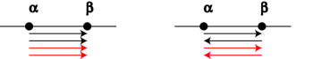
Figure 5: Configurations of $2$ points and $4$ segments on $1$ real line, from Example 6.4. Left: configuration $\mathcal{S}$; Right: configuration $\mathcal{T}$.

Now, let $\mathcal{T}$ be a new weight $(2,2)$ h-configuration: the same line $L$ and points $\alpha$, $\beta$ as $\mathcal{S}$, but with two black segments in opposite directions, and two red segments also in opposite directions. The indexing as in (17) is $\mathcal{T}=(\mathcal{T}_{0},\mathcal{T}_{1})$, $\mathcal{T}_{0}=\mathcal{T}_{1}=[(\alpha,\beta),(\beta,\alpha)]$. There is obviously no morphism $\mathcal{S}\to\mathcal{T}$, and the weighted invariant is a different element of $\mathbb{R}P(2,2)$:

$$E_{(2,2)}(\mathcal{T})=\left[\llbracket\overrightarrow{\alpha\beta}\rrbracket\llbracket\overrightarrow{\beta\alpha}\rrbracket:\llbracket\overrightarrow{\alpha\beta}\rrbracket\llbracket\overrightarrow{\beta\alpha}\rrbracket\right]_{(2,2)}=[-1:-1]_{(2,2)}.$$

$\mathcal{T}$ is also a weight $(1,1)$ h-configuration, with $(1,1)$ invariant:

$$E_{(1,1)}(\mathcal{T}^{(0,1)}) = h_{0,1}(E_{(2,2)}(\mathcal{T}))$$

$$= \left[\llbracket\overrightarrow{\alpha\beta}\rrbracket\llbracket\overrightarrow{\beta\alpha}\rrbracket:\llbracket\overrightarrow{\alpha\beta}\rrbracket\llbracket\overrightarrow{\beta\alpha}\rrbracket\right]_{(1,1)}$$

$$= [-1:-1]=[1:1].$$

The conclusion is that the $E_{(1,1)}$ invariant cannot distinguish between $\mathcal{S}^{(0,1)}=\mathcal{S}$ and $\mathcal{T}^{(0,1)}=\mathcal{T}$.

Example 6.5.

Let $\alpha$, $\beta$, $\gamma$ be the vertices of a triangle in the Euclidean plane $\mathbb{R}^{2}$, and let $\alpha^{\prime}$, $\beta^{\prime}$, $\gamma^{\prime}$ be the midpoints on opposite sides. The following $((2,2,4),2,3,2)$-configuration $\mathcal{S}=(\mathcal{S}_{0},\mathcal{S}_{1},\mathcal{S}_{2})$ is a weight $(2,2,4)$ h-configuration.

$$\mathcal{S}_{0} = [(\beta,\alpha^{\prime}),(\beta,\alpha^{\prime}),(\gamma,\beta^{\prime}),(\gamma,\beta^{\prime}),(\alpha,\gamma^{\prime}),(\alpha,\gamma^{\prime})]$$

$$\mathcal{S}_{1} = [(\alpha^{\prime},\gamma),(\alpha^{\prime},\gamma),(\beta^{\prime},\alpha),(\beta^{\prime},\alpha),(\gamma^{\prime},\beta),(\gamma^{\prime},\beta)]$$

$$\mathcal{S}_{2} = [(\beta,\alpha^{\prime}),(\beta,\alpha^{\prime}),(\alpha^{\prime},\gamma),(\alpha^{\prime},\gamma),(\gamma,\beta^{\prime}),(\gamma,\beta^{\prime}),$$

$$\ (\beta^{\prime},\alpha),(\beta^{\prime},\alpha),(\alpha,\gamma^{\prime}),(\alpha,\gamma^{\prime}),(\gamma^{\prime},\beta),(\gamma^{\prime},\beta)].$$

It is possible to pick a direction and unit of length for each of the three lines so all the directed segments have signed length $+1$. The invariant from Corollary 5.1 is:

$$E_{\mathbf{p}}(\mathcal{S}) = [1:1:1]_{(2,2,4)}.$$

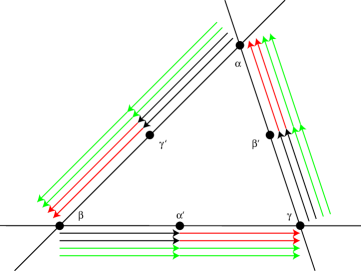
Figure 6: The configuration $\mathcal{S}$ from Example 6.5, of $6$ points, $3$ lines, and $24$ directed segments in the real plane.

If we ignore the green segments and look only at the black and red segments, $\mathcal{S}^{(0,1)}=(\mathcal{S}_{0},\mathcal{S}_{1})$ is an h-configuration with $E_{(1,1)}(\mathcal{S}^{(0,1)})=[1:1]$. However, the other color pairs $(\mathcal{S}_{0},\mathcal{S}_{2})$ and $(\mathcal{S}_{1},\mathcal{S}_{2})$ are not h-configurations. The modification of $(\mathcal{S}_{0},\mathcal{S}_{2})$ into $\mathcal{S}^{(0,2)}$ is to duplicate all the black segments, so each line has four black segments and four green segments. Then $E_{(1,1)}(\mathcal{S}^{(0,2)})=[1:1]$ as in Corollary 6.3, and similarly $E_{(1,1)}(\mathcal{S}^{(1,2)})=[1:1]$.

By Theorems 2.12 and 3.11, the product of axis projections,

$$\prod h_{ij}:\mathbb{R}P(2,2,4) \to \mathbb{R}P^{1}\times\mathbb{R}P^{1}\times\mathbb{R}P^{1}:$$

$$z \mapsto (h_{01}(z),h_{02}(z),h_{12}(z)),$$

$$[z_{0}:z_{1}:z_{2}]_{(2,2,4)} \mapsto ([z_{1}:z_{2}],[z_{0}^{2}:z_{2}],[z_{1}^{2}:z_{2}]),$$

is two-to-one on $D_{\mathbf{p}}$. In particular, $[1:1:1]_{(2,2,4)}\mapsto([1:1],[1:1],[1:1])$, and the other point with that image is $[-1:-1:1]_{(2,2,4)}$.

So, as in Example 6.4, it is possible to find projectively inequivalent weight $(2,2,4)$ h-configurations $\mathcal{S}$ and $\mathcal{T}$ with different $E_{(2,2,4)}$ invariants, but which have the same $E_{(1,1)}$ invariants from applying Eves’ Theorem to their three h-configurations $\mathcal{S}^{(i,j)}$ and $\mathcal{T}^{(i,j)}$. We can reverse some of the red and black directed segments from $\mathcal{S}$ to get a new configuration $\mathcal{T}=(\mathcal{T}_{0},\mathcal{T}_{1},\mathcal{T}_{2})$,

$$\mathcal{T}_{0} = [(\beta,\alpha^{\prime}),(\alpha^{\prime},\beta),(\gamma,\beta^{\prime}),(\beta^{\prime},\gamma),(\alpha,\gamma^{\prime}),(\gamma^{\prime},\alpha)]$$

$$\mathcal{T}_{1} = [(\alpha^{\prime},\gamma),(\gamma,\alpha^{\prime}),(\beta^{\prime},\alpha),(\alpha,\beta^{\prime}),(\gamma^{\prime},\beta),(\beta,\gamma^{\prime})]$$

$$\mathcal{T}_{2} = \mathcal{S}_{2}.$$

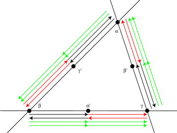
Figure 7: The configuration $\mathcal{T}$ from Example 6.5.

So, $E_{\mathbf{p}}(\mathcal{T})=[-1:-1:1]_{(2,2,4)}$, and all three $(i,j)$ color pairs have $E_{(1,1)}(\mathcal{T}^{(i,j)})=[1:1]$.

The next Example is a configuration considered by [B]; all six points are in the Euclidean plane, as in Examples 5.2, 5.3, but the configuration can be seen to have an octahedral pattern.

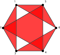
Figure 8: A configuration of $6$ points in the real plane, showing the $4$ red triangles from Example 6.6.

Example 6.6.

Let ${\mathnormal{1}},{\mathnormal{2}},{\mathnormal{3}},{\mathnormal{4}},{\mathnormal{5}},{\mathnormal{6}}$, be six points in the Euclidean plane as in Example 5.2. Let $\mathcal{S}=(\mathcal{S}_{0},\mathcal{S}_{1})$ be a configuration of four black triangles and four red triangles:

$$\mathcal{S}_{0} = [\triangle({\mathnormal{4}}{\mathnormal{6}}{\mathnormal{5}}),\triangle({\mathnormal{4}}{\mathnormal{2}}{\mathnormal{3}}),\triangle({\mathnormal{5}}{\mathnormal{1}}{\mathnormal{2}}),\triangle({\mathnormal{1}}{\mathnormal{3}}{\mathnormal{6}})],$$

$$\mathcal{S}_{1} = [\triangle({\mathnormal{1}}{\mathnormal{2}}{\mathnormal{3}}),\triangle({\mathnormal{1}}{\mathnormal{6}}{\mathnormal{5}}),\triangle({\mathnormal{2}}{\mathnormal{4}}{\mathnormal{5}}),\triangle({\mathnormal{3}}{\mathnormal{4}}{\mathnormal{6}})].$$

Each of the six points has black degree and red degree equal to $2$, so, unlike Example 5.2, $\mathcal{S}$ can be viewed as either a $((2,2),3,2,2)$-configuration or a $((1,1),3,4,2)$-configuration. $\mathcal{S}$ is both a weight $(2,2)$ h-configuration and a weight $(1,1)$ h-configuration, equal to $\mathcal{S}^{(0,1)}$. In the plane coordinate system from Section 5, the $(2,2)$ invariant is:

$$E_{(2,2)}(\mathcal{S}) = \left[\llbracket\triangle({\mathnormal{4}}{\mathnormal{6}}{\mathnormal{5}})\rrbracket_{\mathcal{B}}\llbracket\triangle({\mathnormal{4}}{\mathnormal{2}}{\mathnormal{3}})\rrbracket_{\mathcal{B}}\llbracket\triangle({\mathnormal{5}}{\mathnormal{1}}{\mathnormal{2}})\rrbracket_{\mathcal{B}}\llbracket\triangle({\mathnormal{1}}{\mathnormal{3}}{\mathnormal{6}})\rrbracket_{\mathcal{B}}:\right.$$

$$\ \left.\llbracket\triangle({\mathnormal{1}}{\mathnormal{2}}{\mathnormal{3}})\rrbracket_{\mathcal{B}}\llbracket\triangle({\mathnormal{1}}{\mathnormal{6}}{\mathnormal{5}})\rrbracket_{\mathcal{B}}\llbracket\triangle({\mathnormal{2}}{\mathnormal{4}}{\mathnormal{5}})\rrbracket_{\mathcal{B}}\llbracket\triangle({\mathnormal{3}}{\mathnormal{4}}{\mathnormal{6}})\rrbracket_{\mathcal{B}}\right]_{(2,2)}$$

$$= [z_{0}:z_{1}]_{(2,2)}.$$

The $(1,1)$ invariant of the same configuration is:

$$E_{(1,1)}(\mathcal{S}^{(0,1)})=[z_{0}:z_{1}]_{(1,1)},$$

which can be interpreted as the ratio of signed areas:

$$\frac{z_{1}}{z_{0}}=\frac{(Area\triangle({\mathnormal{1}}{\mathnormal{2}}{\mathnormal{3}}))(Area\triangle({\mathnormal{1}}{\mathnormal{6}}{\mathnormal{5}}))(Area\triangle({\mathnormal{2}}{\mathnormal{4}}{\mathnormal{5}}))(Area\triangle({\mathnormal{3}}{\mathnormal{4}}{\mathnormal{6}}))}{(Area\triangle({\mathnormal{4}}{\mathnormal{6}}{\mathnormal{5}}))(Area\triangle({\mathnormal{4}}{\mathnormal{2}}{\mathnormal{3}}))(Area\triangle({\mathnormal{5}}{\mathnormal{1}}{\mathnormal{2}}))(Area\triangle({\mathnormal{1}}{\mathnormal{3}}{\mathnormal{6}}))}.$$

We remark that the property $E_{(1,1)}(\mathcal{S}^{(0,1)})=[1:1]$ is equivalent to the projective property that six points lie on a conic ([CRG], [RG]).

Let $\mathcal{T}=(\mathcal{T}_{0},\mathcal{T}_{1})$ be a new configuration — the same six points, but changing the order of points in one of the black triangles and one of the red triangles to get the opposite signed areas:

$$\mathcal{T}_{0} = [\triangle({\mathnormal{4}}{\mathnormal{5}}{\mathnormal{6}}),\triangle({\mathnormal{4}}{\mathnormal{2}}{\mathnormal{3}}),\triangle({\mathnormal{5}}{\mathnormal{1}}{\mathnormal{2}}),\triangle({\mathnormal{1}}{\mathnormal{3}}{\mathnormal{6}})],$$

$$\mathcal{T}_{1} = [\triangle({\mathnormal{1}}{\mathnormal{3}}{\mathnormal{2}}),\triangle({\mathnormal{1}}{\mathnormal{6}}{\mathnormal{5}}),\triangle({\mathnormal{2}}{\mathnormal{4}}{\mathnormal{5}}),\triangle({\mathnormal{3}}{\mathnormal{4}}{\mathnormal{6}})].$$

Then $\mathcal{T}$ has the same $E_{(1,1)}$ invariant, and in the ratio of signed areas, the sign changes cancel, giving the same ratio as $\mathcal{S}$. The two configurations have different $(2,2)$ invariants, so they are projectively inequivalent:

$$E_{(2,2)}(\mathcal{T})=[-z_{0}:-z_{1}]_{(2,2)}\neq[z_{0}:z_{1}]_{(2,2)}=E_{(2,2)}(\mathcal{S}).$$

Acknowledgments

The author was motivated to start writing this paper after attending a talk by M. Frantz ([F₁]), and he thanks Frantz for subsequent conversations and for pointing out the reference [P]. The Figures were generated using [Ai].

References

- [Ai] Adobe Illustrator CS5, Version 15.0.0.
- [BBR] M. Barnabei, A. Brini, and G.-C. Rota, On the exterior calculus of invariant theory, J. Algebra (1) 96 (1985), 120–160. MR0808845 (87j:05002).
- [B] J. Brill, On certain analogues of anharmonic ratio, Quarterly J. Pure and Appl. Math. 29 (1898), 286–302.
- [BB] M. Brill and E. Barrett, Closed-form extension of the anharmonic ratio to -space, Computer Vision, Graphics, and Image Processing (1) 23 (1983), 92–98.
- [C] W. Clifford, Analytical metrics, Quarterly J. Pure and Appl. Math. (25) 7 (1865), (29) 8 (1866), (30) 8 (1866); reprinted in Mathematical Papers by William Kingdon Clifford, R. Tucker, ed., Chelsea, New York, 1968. MR 0238662 (39 #26).
- [CRG] H. Crapo and J. Richter-Gebert, Automatic proving of geometric theorems, Invariant Methods in Discrete and Computational Geometry, 167–196, N. White, ed., Kluwer, 1995. MR 1368011 (97b:68196).
- [Delorme] C. Delorme, Espaces projectifs anisotropes, Bull. Soc. Math. France (2) 103 (1975), 203–223. MR 0404277 (53 #8080a).
- [Dolgachev] I. Dolgachev, Weighted projective varieties, Group Actions and Vector Fields (Vancouver, B.C., 1981), 34–71, LNM 956, Springer, Berlin, 1982. MR 0704986 (85g:14060).
- [E] H. Eves, A Survey of Geometry, Revised Ed., Allyn & Bacon, Boston, 1972. MR 0322653 (48 #1015).
- [F1] M. Frantz, “The most underrated theorem in projective geometry,” presentation at the 2011 MAA MathFest, Lexington, KY, August 6, 2011.
- [F2] M. Frantz, A car crash solved — with a Swiss Army knife, Mathematics Magazine (5) 84 (2011), 327–338.
- [O] Ø. Ore, Number Theory and its History, McGraw-Hill, New York, 1948. MR 0026059 (10,100b).
- [P] J.-V. Poncelet, Traité des Propriétés Projectives des Figures, Ed., Bachelier, Paris, 1822.
- [RG] J. Richter-Gebert, Perspectives on Projective Geometry, Springer, Berlin, 2011. MR 2791970.
- [Salmon] G. Salmon, Lessons Introductory to the Modern Higher Algebra, Ed., Chelsea, New York, 1885.
- [Shephard] G. Shephard, Isomorphism invariants for projective configurations, Canad. J. Math. (6) 51 (1999), 1277–1299. MR 1756883 (2001d:51014).