Density-sensitive semisupervised inference

Abstract

Semisupervised methods are techniques for using labeled data $(X_{1},Y_{1}),\ldots,(X_{n},Y_{n})$ together with unlabeled data $X_{n+1},\ldots,X_{N}$ to make predictions. These methods invoke some assumptions that link the marginal distribution $P_{X}$ of $X$ to the regression function $f(x)$. For example, it is common to assume that $f$ is very smooth over high density regions of $P_{X}$. Many of the methods are ad-hoc and have been shown to work in specific examples but are lacking a theoretical foundation. We provide a minimax framework for analyzing semisupervised methods. In particular, we study methods based on metrics that are sensitive to the distribution $P_{X}$. Our model includes a parameter $\alpha$ that controls the strength of the semisupervised assumption. We then use the data to adapt to $\alpha$.

, and

t2Supported by Air Force Grant FA9550-10-1-0382 and NSF Grant IIS-1116458.

t3Supported by NSF Grant DMS-08-06009 and Air Force Grant FA95500910373.

1 Introduction

Suppose we have data $(X_{1},Y_{1}),\ldots,(X_{n},Y_{n})$ from a distribution $P$, where $X_{i}\in\mathbb{R}^{d}$ and $Y_{i}\in\mathbb{R}$. Further, we have a second set of data $X_{n+1},\ldots,X_{N}$ from the same distribution but without the $Y$’s. We refer to ${\cal L}=\{(X_{i},Y_{i})\dvtx i=1,\ldots,n\}$ as the labeled data and ${\cal U}=\{X_{i}\dvtx i=n+1,\ldots,N\}$ as the unlabeled data. There has been a major effort, mostly in the machine learning literature, to find ways to use the unlabeled data together with the labeled data to constuct good predictors of $Y$. These methods are known as semisupervised methods. It is generally assumed that the $m=N-n$ unobserved labels $Y_{n+1},\ldots,Y_{N}$ are missing completely at random and we shall assume this throughout.

To motivate semisupervised inference, consider the following example. We download a large number $N$ of webpages $X_{i}$. We select a small subset of size $n$ and label these with some attribute $Y_{i}$. The downloading process is cheap whereas the labeling process is expensive so typically $N$ is huge while $n$ is much smaller.

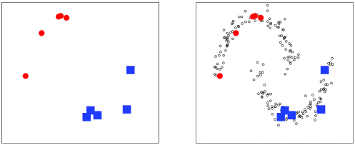
Figure 1: The covariate $X=(X_{1},X_{2})$ is two dimensional. The response $Y$ is binary and is shown as a square or a circle. Left: the labeled data. Right: labeled and unlabeled data.

Figure 1 shows a toy example of how unlabeled data can help with prediction. In this case, $Y$ is binary, $X\in\mathbb{R}^{2}$ and we want to find the decision boundary $\{x\dvtx P(Y=1|X=x)=1/2\}$. The left plot shows a few labeled data points from which it would be challenging to find the boundary. The right plot shows labeled and unlabeled points. The unlabeled data show that there are two clusters. If we make the seemingly reasonable assumption that $f(x)=P(Y=1|X=x)$ is very smooth over the two clusters, then identifying the decision boundary becomes much easier. In other words, if we assume some link between $P_{X}$ and $f$, then we can use the unlabeled data; see Figure 2.

$${\cal L}_{n}\ \Longrightarrow\ \widehat{f}\hskip 72.26999pt{\cal L}_{n}\ \Longrightarrow\ \widehat{f}\ \stackrel{{\scriptstyle\mathsf{SS}\ \mathsf{assumption}}}{{\Longleftarrow\!=\!=\!=\!=}}\widehat{P}_{X}\Longleftarrow{\cal U}_{N}$$

Figure 2: Supervised learning (left) uses only the labeled data ${\cal L}_{n}$. Semisupervised learning (right) uses the unlabeled data ${\cal U}_{N}$ to estimate the marginal distribution $P_{X}$ which helps estimate $f$ if there is some link between $P_{X}$ and $f$. This link is the semisupervised (SS) assumption.

The assumption that the regression function $f(x)=\mathbb{E}(Y|X=x)$ is very smooth over the clusters is known as the cluster assumption. In the special case where the clusters are low-dimensional submanifolds, the assumption is called the manifold assumption. These assumptions link the regression function $f$ to the distribution $P_{X}$ of $X$.

Many semisupervised methods are developed based on the above assumptions, although this is not always made explicit. Even with such a link, it is not obvious that semisupervised methods will outperform supervised methods. Making precise how and when these assumptions actually improve inferences is surprisingly elusive, and most papers do not address this issue; some exceptions are Rigollet (2007), Singh, Nowak and Zhu (2008), Lafferty and Wasserman (2007), Nadler, Srebro and Zhou (2009), Ben-David, Lu and Pal (2008), Sinha and Belkin (2009), Belkin and Niyogi (2004) and Niyogi (2008). These authors have shown that the degree to which unlabeled data improves performance is very sensitive to the cluster and manifold assumptions. In this paper, we introduce adaptive semisupervised inference. We define a parameter $\alpha$ that controls the sensitivity of the distance metric to the density, and hence the strength of the semisupervised assumption. When $\alpha=0$ there is no semisupervised assumption, that is, there is no link between $f$ and $P_{X}$. When $\alpha=\infty$ there is a very strong semisupervised assumption. We use the data to estimate $\alpha$, and hence we adapt to the appropriate assumption linking $f$ and $P_{X}$. In addition, we should add that we focus on regression while most previous literature only deals with binary outcomes (classification).

This paper makes the following contributions: [(6)]

We formalize the link between the regression function $f$ and the marginal distribution $P_{X}$ by defining a class of function spaces based on a metric that depends on $P_{X}$. This is called a density sensitive metric.

We show how to consistently estimate the density-sensitive metric.

We propose a semi-supervised kernel estimator based on the density-sensitive metric.

We provide some minimax bounds and show that under some conditions the semisupervised method has smaller predictive risk than any supervised method.

The function classes depend on a parameter $\alpha$ that controls how strong the semisupervised assumption is. We show that it is possible to adapt to $\alpha$.

We provide numerical simulations to support the theory.

We now give an informal statement of our main results. In Section 5 we define a nonparametric class of distributions ${\cal P}_{n}$. Let $0<\xi<d-3$ and assume that $m\geq n^{2/(2+\xi)}$. Let ${\cal S}_{n}$ denote the set of supervised estimators; these estimators use only the labeled data. Let ${\cal SS}_{N}$ denote the set of semisupervised estimators; these estimators use the labeled data and unlabeled data. Then: [(3)]

(Theorem 4.1 and Corollary 4.2.) There is a semisupervised estimator $\widehat{f}$ such that

$$\sup_{P\in{\cal P}_{n}}R_{P}(\widehat{f})\leq\biggl{(}\frac{C}{n}\biggr{)}^{{2}/({2+\xi})},$$ (1)

where $R_{P}(\widehat{f})$ is the risk of the estimator $\widehat{f}$ under distribution $P$.

(Theorem 5.1.) For supervised estimators ${\cal S}_{n}$ we have

$$\inf_{\widehat{f}\in{\cal S}_{n}}\sup_{P\in{\cal P}_{n}}R_{P}(\widehat{f})\geq\biggl{(}\frac{C}{n}\biggr{)}^{{2}/({d-1})}.$$ (2)

Combining these two results we conclude that

$$\frac{\inf_{\widehat{f}\in{\cal SS}_{N}}\sup_{P\in{\cal P}_{n}}R_{P}(\widehat{f})}{\inf_{\widehat{f}\in{\cal S}_{n}}\sup_{P\in{\cal P}_{n}}R_{P}(\widehat{f})}\leq\biggl{(}\frac{C}{n}\biggr{)}^{{2(d-3-\xi)}/({(2+\xi)(d-1)})}\to 0$$ (3)

and hence, semisupervised estimation dominates supervised estimation.

We assume, as is standard in the literature on semisupervised learning, that the margial $P_{X}$ is the same for the labeled and unlabeled data. Extensions to the case where the marginal distribution changes are possible, but are beyond the scope of the paper.

Related work. There are a number of papers that discuss conditions under which semisupervised methods can succeed or that discuss metrics that are useful for semisupervised methods. These include Castelli and Cover (1995, 1996), Ratsaby and Venkatesh (1995), Bousquet, Chapelle and Hein (2004), Singh, Nowak and Zhu (2008), Lafferty and Wasserman (2007), Sinha and Belkin (2009), Ben-David, Lu and Pal (2008), Nadler, Srebro and Zhou (2009), Sajama and Orlitsky (2005), Bijral, Ratliff and Srebro (2011), Belkin and Niyogi (2004), Niyogi (2008) and references therein. Papers on semisupervised inference in the statistics literature are rare; some exceptions include Culp and Michailidis (2008), Culp (2011a) and Liang, Mukherjee and West (2007). To the best of our knowledge, there are no papers that explicitly study adaptive methods that allow the data to choose the strength of the semisupervised assumption.

There is a connection between our work on the semisupervised classification method in Rigollet (2007). He divides the covariate space ${\cal X}$ into clusters $C_{1},\ldots,C_{k}$ defined by the upper level sets $\{p_{X}>\lambda\}$ of the density $p_{X}$ of $P_{X}$. He assumes that the indicator function $I(x)=I(p(y|x)>1/2)$ is constant over each cluster $C_{j}$. In our regression framework, we could similarly assume that

$$f(x)=\sum_{j=1}^{k}f_{\theta_{j}}(x)I(x\in C_{j})+g(x)I(x\in C_{0}),$$

where $f_{\theta}(x)$ is a parametric regression function, $g$ is a smooth (but nonparametric function) and $C_{0}={\cal X}-\bigcup_{j=1}^{k}C_{j}$. This yields parametric, dimension-free rates over ${\cal X}-C_{0}$. However, this creates a rather unnatural and harsh boundary at $\{x\dvtx p_{X}(x)=\lambda\}$. Also, this does not yield improved rates over $C_{0}$. Our approach may be seen as a smoother version of this idea.

Outline. This paper is organized as follows. In Section 2 we give definitions and assumptions. In Section 3 we define density sensitive metrics and the function spaces defined by these metrics. In Section 4 we define a density sensitive semisupervised estimator, and we bound its risk. In Section 5 we present some minimax results. We discuss adaptation in Section 6. We provide simulations in Section 7. Section 8 contains the closing discussion. Many technical details and extensions are contained in the supplemental article [Azizyan, Singh and Wasserman (2013)].

2 Definitions

Recall that $X_{i}\in\mathbb{R}^{d}$ and $Y_{i}\in\mathbb{R}$. Let

$${\cal L}_{n}=\bigl{\{}(X_{1},Y_{1}),\ldots,(X_{n},Y_{n})\bigr{\}}$$ (4)

be an i.i.d. sample from $P$. Let $P_{X}$ denote the $X$-marginal of $P$, and let

$${\cal U}_{N}=\{X_{n+1},\ldots,X_{N}\}$$ (5)

be an i.i.d. sample from $P_{X}$.

Let $f(x)\equiv f_{P}(x)=\mathbb{E}(Y|X=x)$. An estimator of $f$ that is a function of ${\cal L}_{n}$ is called a supervised learner, and the set of such estimators is denoted by ${\cal S}_{n}$. An estimator that is a function of ${\cal L}_{n}\cup{\cal U}_{N}$ is called a semisupervised learner, and the set of such estimators is denoted by ${\cal SS}_{N}$. Define the risk of an estimator $\widehat{f}$ by

$$R_{P}(\widehat{f})=\mathbb{E}_{P}\biggl{[}\int\bigl{(}\widehat{f}(x)-f_{P}(x)\bigr{)}^{2}\,dP(x)\biggr{]},$$ (6)

where $\mathbb{E}_{P}$ denotes the expectation over data drawn from the distribution $P$. Of course, ${\cal S}_{n}\subset{\cal SS}_{N}$ and hence

$$\inf_{\widehat{g}\in{\cal SS}_{N}}\sup_{P\in{\cal P}}R_{P}(\widehat{g})\leq\inf_{\widehat{g}\in{\cal S}_{n}}\sup_{P\in{\cal P}}R_{P}(\widehat{g}).$$

We will show that, under certain conditions, semisupervised methods outperform supervised methods in the sense that the left-hand side of the above equation is substantially smaller than the right-hand side. More precisely, for certain classes of distributions ${\cal P}_{n}$, we show that

$$\frac{\inf_{\widehat{g}\in{\cal SS}_{N}}\sup_{P\in{\cal P}_{n}}R_{P}(\widehat{g})}{\inf_{\widehat{g}\in{\cal S}_{n}}\sup_{P\in{\cal P}_{n}}R_{P}(\widehat{g})}\to 0$$ (7)

as $n\to\infty$. In this case we say that semisupervised learning is effective.

In order for the asymptotic analysis to reflect the behavior of finite samples, we need to let ${\cal P}_{n}$ to change with $n$, and we need $N=N(n)\to\infty$ and $n/N(n)\to 0$ as $n\to\infty$. As an analogy, one needs to let the number of covariates in a regression problem increase with the sample size to develop relevant asymptotics for high-dimensional regression. Moreover, ${\cal P}_{n}$ must have distributions that get more concentrated as $n$ increases. The reason is that if $n$ is very large and $P_{X}$ is smooth, then there is no advantage to semisupervised inference. This is consistent with the finding in Ben-David, Lu and Pal (2008) who show that if $P_{X}$ is smooth, then “$\ldots$ knowledge of that distribution cannot improve the labeled sample complexity by more than a constant factor.”

Other notation. If $A$ is a set and $\delta\geq 0$, we define

$$A\oplus\delta=\bigcup_{x\in A}B(x,\delta),$$

where $B(x,\delta)$ denotes a ball of radius $\delta$ centered at $x$. Given a set $A\subseteq\mathbb{R}^{d}$, define $d_{A}(x_{1},x_{2})$ to be the length of the shortest path in $A$ connecting $x_{1}$ and $x_{2}$.

We write $a_{n}=O(b_{n})$ if $|a_{n}/b_{n}|$ is bounded for all large $n$. Similarly, $a_{n}=\Omega(b_{n})$ if $|a_{n}/b_{n}|$ is bounded away from 0 for all large $n$. We write $a_{n}\asymp b_{n}$ if $a_{n}=O(b_{n})$ and $a_{n}=\Omega(b_{n})$. We also write $a_{n}\preceq b_{n}$ if there exists $C>0$ such that $a_{n}\leq Cb_{n}$ for all large $n$. Define $a_{n}\succeq b_{n}$ similarly. We use symbols of the form $c,c_{1},c_{2},\ldots,C,C_{1},C_{2},\ldots$ to denote generic positive constants whose value can change in different expressions.

3 Density-sensitive function spaces

We define a smoothed version of $P_{X}$ as follows. (This is needed since we allow the marginal distribution $P_{X}$ to be singular.) Let $K$ denote a symmetric kernel on $\mathbb{R}^{d}$ with compact support, let $\sigma>0$ and define

$$p_{\sigma}(x)\equiv p_{X,\sigma}(x)=\int\frac{1}{\sigma^{d}}K\biggl{(}\frac{\|x-u\|}{\sigma}\biggr{)}\,dP_{X}(x).$$ (8)

Thus, $p_{X,\sigma}$ is the density of the convolution $P_{X,\sigma}=P_{X}\star\mathbb{K}_{\sigma}$ where $\mathbb{K}_{\sigma}$ is the measure with density $K_{\sigma}(\cdot)=\sigma^{-d}K(\cdot/\sigma)$. $P_{X,\sigma}$ always has a density even if $P_{X}$ does not. This is important because, in high-dimensional problems, it is not uncommon to find that $P_{X}$ can be highly concentrated near a low-dimensional manifold. These are precisely the cases where semisupervised methods are often useful [Ben-David, Lu and Pal (2008)]. Indeed, this was one of the original motivations for semisupervised inference. We define $P_{X,0}=P_{X}$. For notational simplicity, we shall sometimes drop the $X$ and simply write $p_{\sigma}$ instead of $p_{X,\sigma}$.

3.1 The exponential metric

Following previous work in the area, we will assume that the regression function is smooth in regions where $P_{X}$ puts lots of mass. To make this precise, we define a density sensitive metric as follows. For any pair $x_{1}$ and $x_{2}$ let $\Gamma(x_{1},x_{2})$ denote the set of all continuous finite curves from $x_{1}$ to $x_{2}$ with unit speed everywhere, and let $L(\gamma)$ be the length of curve $\gamma$; hence $\gamma(L(\gamma))=x_{2}$. For any $\alpha\geq 0$ define the exponential metric

$$D(x_{1},x_{2})\equiv D_{P,\alpha,\sigma}(x_{1},x_{2})=\inf_{\gamma\in\Gamma(x_{1},x_{2})}\int_{0}^{L(\gamma)}\exp\bigl{[}-\alpha p_{X,\sigma}\bigl{(}\gamma(t)\bigr{)}\bigr{]}\,dt.$$ (9)

In the supplement, we also consider a second metric, the reciprocal metric. Large $\alpha$ makes points connected by high density paths closer; see Figure 3.

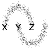
Figure 3: With a density metric, the points $X$ and $Z$ are closer than the points $X$ and $Y$ because there is a high density path connecting $X$ and $Z$.

Note that $\alpha=0$ corresponds to Euclidean distance. Similar definitions are used in Sajama and Orlitsky (2005), Bijral, Ratliff and Srebro (2011) and Bousquet, Chapelle and Hein (2004).

3.2 The regression function

Recall that $f(x)\equiv f_{P}(x)=E(Y|X=x)$ denotes the regression function. We assume that $X\in[0,1]^{d}\equiv{\cal X}$ and that $|Y|\leq M$ for some finite constant $M$. We formalize the semisupervised smoothness assumption by defining the following scale of function spaces. Let ${\cal F}\equiv{\cal F}(P,\alpha,\sigma,L)$ denote the set functions $f\dvtx[0,1]^{d}\to\mathbb{R}$ such that, for all $x_{1},x_{2}\in{\cal X}$,

$$\bigl{|}f(x_{1})-f(x_{2})\bigr{|}\leq LD_{P,\alpha,\sigma}(x_{1},x_{2}).$$ (10)

Let ${\cal P}(\alpha,\sigma,L)$ denote all joint distributions for $(X,Y)$ such that $f_{P}\in{\cal F}(P,\alpha,\break\sigma,L)$ and such that $P_{X}$ is supported on ${\cal X}$.

3.3 Properties of the function spaces

Let $B_{P,\alpha,\sigma}(x,\varepsilon)=\{z\dvtx D_{P,\alpha,\sigma}(x,\break z)\leq\varepsilon\}$ be a ball of size $\varepsilon$. Let $S_{P}$ denote the support of $P$, and let ${\cal N}_{P,\alpha,\sigma}(\varepsilon)$ denote the covering number, the smallest number of balls of size $\varepsilon$ required to cover $S_{P}$. The covering number measures the size of the function space, and the variance of any regression estimator on the space ${\cal F}(P,\alpha,\sigma,L)$ depends on this covering number. Here, we mention a few properties of ${\cal N}_{P,\alpha,\sigma}(\varepsilon)$.

In the Euclidean case $\alpha=0$, we have ${\cal N}_{P,0,\sigma}(\varepsilon)\leq(C/\varepsilon)^{d}$. But when $\alpha>0$ and $P$ is concentrated on or near a set of dimension less than $d$, the ${\cal N}_{P,\alpha,\sigma}(\varepsilon)$ can be much smaller than $(C/\varepsilon)^{d}$. The next result gives a few examples showing that concentrated distributions have small covering numbers. We say that a set $A$ is regular if there is a $C>0$ such that, for all small $\varepsilon>0$,

$$\sup_{\stackrel{{\scriptstyle x,y\in A}}{{\|x-y\|\leq\varepsilon}}}\frac{d_{A}(x,y)}{\|x-y\|}\leq C,$$ (11)

where $d_{A}(x_{1},x_{2})$ is the length of the shortest path in $A$ connecting $x_{1}$ and $x_{2}$. Recall that $S_{P}$ denotes the support of $P$.

Lemma 1

Suppose that $S_{P}$ is regular. [(4)]

For all $\alpha$, $\sigma$ and $P$, ${\cal N}_{P,\alpha,\sigma}(\varepsilon)\preceq\varepsilon^{-d}$.

Suppose that $P=\sum_{j=1}^{k}\delta_{x_{j}}$ where $\delta_{x}$ is a point mass at $x$. Then, for any $\alpha\geq 0$ and any $\varepsilon>0$, ${\cal N}_{P,\alpha,\sigma}(\varepsilon)\leq k$.

Suppose that $\mathsf{dim}(S_{P})=r<d$. Then, ${\cal N}_{P,\alpha,\sigma}(\varepsilon)\preceq\varepsilon^{-r}$.

Suppose that $S_{P}=W\oplus\gamma$ where $\mathsf{dim}(W)=r<d$. Then, for $\varepsilon\geq C\gamma$, ${\cal N}_{P,\alpha,\sigma}(\varepsilon)\preceq(\frac{1}{\varepsilon})^{r}$.

(1) The first statement follows since the covering number of $S_{P}$ is no more than the covering number of $[0,1]^{d}$ and on $[0,1]^{d}$, $D_{P,\alpha,\sigma}(x,y)\leq\|x-y\|$. Now $[0,1]^{d}$ can be covered $O(\varepsilon^{-d})$ Euclidean balls.

(2) The second statement follows since $\{\{x_{1}\},\ldots,\{x_{k}\}\}$ forms an $\varepsilon$-covering for any $\varepsilon$.

(3) We have that $D_{P,\alpha,\sigma}(x,y)\leq d_{S_{P}}(x,y)$. Regularity implies that, for small $d_{S_{P}}(x,y)$, $D_{P,\alpha,\sigma}(x,y)\leq c\|x-y\|$. We can thus cover $S_{P}$ by $C\varepsilon^{-r}$ balls of size $\varepsilon$.

(4) As in (3), cover $W$ with $N=O(\varepsilon^{-r})$ balls of $D$ size $\varepsilon$. Denote these balls by $B_{1},\ldots,B_{N}$. Define $C_{j}=\{x\in S_{P}\dvtx d_{S_{P}}(x,B_{j})\leq\gamma\}$. The $C_{j}$ form a covering of size $N$ and each $C_{j}$ has $D_{P,\alpha,\sigma}$ diameter $\max\{\varepsilon,\gamma\}$.

4 Semisupervised kernel estimator

We consider the following semisupervised estimator which uses a kernel that is sensitive to the density. Let $Q$ be a kernel and let $Q_{h}(x)=h^{-d}Q(x/h)$. Let

$$\widehat{f}_{h,\alpha,\sigma}(x)=\frac{\sum^{n}_{i=1}Y_{i}Q_{h}(\widehat{D}_{\alpha,\sigma}(x,X_{i}))}{\sum^{n}_{i=1}Q_{h}(\widehat{D}_{\alpha,\sigma}(x,X_{i}))},$$ (12)

where

$$\widehat{D}_{\alpha,\sigma}(x_{1},x_{2}) = \inf_{\gamma\in\Gamma(x_{1},x_{2})}\int_{0}^{L(\gamma)}\exp\bigl{[}-\alpha\widehat{p}_{\sigma}\bigl{(}\gamma(t)\bigr{)}\bigr{]}\,dt,$$ (13)

$$\widehat{p}_{\sigma}(x) = \frac{1}{m}\sum_{i=1}^{m}\frac{1}{\sigma^{d}}K\biggl{(}\frac{\|x-X_{i+n}\|}{\sigma}\biggr{)},$$ (14)

and $m=N-n$ denotes the number of unlabeled points. We use a kernel estimator for the regression function because it is simple, commonly used and, as we shall see, has a fast rate of convergence in the semisupervised case.

The estimator $\widehat{D}_{\alpha,\sigma}(x_{1},x_{2})$ is discussed in detail in the supplement where we study its properties and we give an algorithm for computing it.

Now we give an upper bound on the risk of $\widehat{f}_{h,\alpha,\sigma}$. In the following we take, for simplicity, $Q(x)=I(\|x\|\leq 1)$.

Theorem 4.1

Suppose that $|Y|\leq M$. Define the event $\mathcal{G}_{m}=\{\|\widehat{p}_{\sigma}-p_{\sigma}\|_{\infty}\leq\varepsilon_{m}\}$ (which depends on the unlabeled data) and suppose that $\mathbb{P}({\cal G}_{m}^{c})\leq 1/m$. Then, for every $P\in{\cal P}(\alpha,\sigma,L)$,

$$R_{P}(\widehat{f}_{h,\alpha,\sigma})\leq L^{2}\bigl{(}he^{\alpha\varepsilon_{m}}\bigr{)}^{2}+\frac{M^{2}(2+{1}/{e}){\cal N}(P,\alpha,\sigma,e^{-\varepsilon_{m}\alpha}h/2)}{n}+\frac{4M^{2}}{m}.$$ (15)

The risk is

$$R_{P}(\widehat{f}) = \mathbb{E}_{n,N}\biggl{[}(1-\mathcal{G}_{m})\int\bigl{(}\widehat{f}_{h,\alpha,\sigma}(x)-f(x)\bigr{)}^{2}\,dP(x)\biggr{]}$$

$${}+\mathbb{E}_{n,N}\biggl{[}\mathcal{G}_{m}\int\bigl{(}\widehat{f}_{h,\alpha,\sigma}(x)-f(x)\bigr{)}^{2}\,dP(x)\biggr{]}.$$

Since $|Y|\leq M$ and $\sup_{x}|\widehat{f}(x)|\leq M$,

$$\mathbb{E}_{n,N}\biggl{[}(1-\mathcal{G}_{m})\int\bigl{(}\widehat{f}_{h,\alpha,\sigma}(x)-f(x)\bigr{)}^{2}\,dP(x)\biggr{]}\leq 4M^{2}\mathbb{P}\bigl{(}\mathcal{G}_{m}^{c}\bigr{)}\leq\frac{4M^{2}}{m}.$$

Now we bound the second term.

Condition on the unlabeled data. Replacing the Euclidean distance with $\widehat{D}_{\alpha,\sigma}$ in the proof of Theorem 5.2 in Györfi et al. (2002), we have that

$$\mathbb{E}_{n}\biggl{[}\int\bigl{(}\widehat{f}_{h,\alpha,\sigma}(x)-f(x)\bigr{)}^{2}\,dP(x)\biggr{]}$$

$$\qquad\leq L^{2}R^{2}+\frac{M^{2}(2+{1}/{e})\int{dP(x)}/{P(\widehat{B}_{\alpha,\sigma}(x,h))}}{n},$$

where

$$R=\sup\bigl{\{}D_{P,\alpha,\sigma}(x_{1},x_{2})\dvtx(x_{1},x_{2})\mbox{ such that }\widehat{D}_{\alpha,\sigma}(x_{1},x_{2})\leq h\bigr{\}}$$

and $\widehat{B}_{\alpha,\sigma}(x,h)=\{z\dvtx\widehat{D}_{\alpha,\sigma}(x,z)\leq h\}$. On the event ${\cal G}_{m}$, we have from Lemma 2 in the supplement that $e^{-\alpha\varepsilon_{m}}D_{\alpha,\sigma}(x_{1},x_{2})\leq\widehat{D}_{\alpha,\sigma}(x_{1},x_{2})\leq e^{\alpha\varepsilon_{m}}D_{\alpha,\sigma}(x_{1},x_{2})$ for all $x_{1},x_{2}$. Hence, $R^{2}\leq e^{2\alpha\varepsilon_{m}}h^{2}$ and

$$\int\frac{dP(x)}{P(\widehat{B}_{\alpha,\sigma}(x,h))}\leq\int\frac{dP(x)}{P(B_{P,\alpha,\sigma}(x,e^{-\alpha\varepsilon_{m}}h))}.$$

A simple covering argument [see page 76 of Györfi et al. (2002)] shows that, for any $\delta>0$,

$$\int\frac{dP(x)}{P(B_{P,\alpha,\sigma}(x,\delta))}\leq{\cal N}(P,\alpha,\sigma,\delta/2).$$

The result follows.

Corollary 4.2

If ${\cal N}(P,\alpha,\sigma,\delta)\leq(C/\delta)^{\xi}$ for $\delta\geq(1/2)e^{-\alpha\varepsilon_{m}}(n\times\break e^{2\alpha\varepsilon_{m}})^{-{1}/({2+\xi})}$ and $N\geq 2n$, then

$$R_{P}(\widehat{f}_{\alpha,\sigma,h})\leq e^{\alpha\varepsilon_{m}(2\vee\xi)}\biggl{[}L^{2}h^{2}+\frac{1}{n}\biggl{(}\frac{C}{h}\biggr{)}^{\xi}\biggr{]}+\frac{4M^{2}}{m}.$$ (16)

Hence, if $m\geq n^{2/(2+\xi)}$ and $h\asymp(ne^{\alpha\varepsilon_{m}(2-\xi)})^{-{1}/({2+\xi})}$, then

$$\sup_{P\in{\cal P}(\alpha,\sigma,L)}R_{P}(\widehat{f}_{h,\alpha,\sigma})\preceq\biggl{(}\frac{C}{n}\biggr{)}^{{2}/({2+\xi})}.$$ (17)

5 Minimax bounds

To characterize when semisupervised methods outperform supervised methods, we show that there is a class of distributions ${\cal P}_{n}$ (which we allow to change with $n$) such that $R_{SS}$ is much smaller than $R_{S}$, where

$$R_{S}=\inf_{\widehat{f}\in{\cal S}_{n}}\sup_{P\in{\cal P}_{n}}R_{P}(\widehat{f})\quad\mbox{and}\quad R_{SS}=\inf_{\widehat{f}\in{\cal SS}_{N}}\sup_{P\in{\cal P}_{n}}R_{P}(\widehat{f}).$$

To do so, it suffices to find a lower bound on $R_{S}$ and an upper bound on $R_{SS}$. Intuitively, ${\cal P}_{n}$ should be a set distributions whose $X$-marginals are highly concentrated on or near lower-dimensional sets, since this is where semisuspervised methods deliver improved performance. Indeed, as we mentioned earlier, for very smooth distributions $P_{X}$ we do not expect semisupervised learners to offer much improvement.

5.1 The class ${\cal P}_{n}$

Here we define the class ${\cal P}_{n}$. Let $N=N(n)$ and $m=m(n)=N-n$ and define

$$\varepsilon_{m}\equiv\varepsilon(m,\sigma)=\sqrt{\frac{C\log m}{m\sigma^{d}}}.$$ (18)

Let $\xi\in[0,d-3)$, $\gamma>0$ and define

$${\cal P}_{n}=\bigcup_{(\alpha,\sigma)\in{\cal A}_{n}\times\Sigma_{n}}{\cal Q}(\alpha,\sigma,L),$$ (19)

where ${\cal Q}(\alpha,\sigma,L)\subset{\cal P}(\alpha,\sigma,L)$ and ${\cal A}_{n}\times\Sigma_{n}\subset[0,\infty]^{2}$ satisfy the following conditions:

$$\mbox{(C1)}\quad{\cal Q}(\alpha,\sigma,L)$$

$$\hphantom{\mbox{(C1)}}\quad\qquad=\biggl{\{}P\in{\cal P}(\alpha,\sigma,L)\dvtx{\cal N}(P,\alpha,\sigma,\varepsilon)\leq\biggl{(}\frac{C}{\varepsilon}\biggr{)}^{\xi}\ \forall\varepsilon\geq\biggl{(}\frac{1}{n}\biggr{)}^{{1}/({2+\xi})}\biggr{\}};$$

$$\mbox{(C2)}\quad\alpha\leq\frac{\log 2}{\varepsilon(m,\sigma)};$$

$$\mbox{(C3)}\quad\biggl{(}\frac{1}{m}\biggr{)}^{{1}/({d(1+\gamma)})}\leq\sigma\leq\frac{1}{4C_{0}}\biggl{(}\frac{1}{n}\biggr{)}^{{1}/({d-1})},$$

where $C_{0}$ is the diameter of the support of $K$.

Here are some remarks about ${\cal P}_{n}$: [(3)]

(C2) implies that $e^{\alpha\varepsilon_{m}}\leq 2$ and hence, (C3) and Theorem 1.3 in the supplement $(1/2)D_{P,\alpha,\sigma}(x_{1},x_{2})\leq\widehat{D}_{\alpha,\sigma}(x_{1},x_{2})\leq 2D_{P,\alpha,\sigma}(x_{1},x_{2})$ with probability at least $1-1/m$.

The constraint in (C1) on ${\cal N}(\varepsilon)$ holds whenever $P$ is concentrated on or near a set of dimension less than $d$ and $\alpha/\sigma^{d}$ is large. The constraint does not need to hold for arbitrarily small $\varepsilon$.

Some papers on semisupervised learning simply assume that $N=\infty$ since in practice $N$ is usually very large compared to $n$. In that case, there is no upper bound on $\alpha$ and no lower bound on $\sigma$.

The class ${\cal P}_{n}$ may seem complicated. This is because showing conditions where semisupervised learning provably outperforms supervised learning is subtle. Intuitively, the class ${\cal P}_{n}$ is simply the set of high concentrated distributions with $\alpha/\sigma$ large.

5.2 Supervised lower bound

Theorem 5.1

Suppose that $m\geq n^{{d(1+\gamma)}/({d-1})}$. There exists $C>0$ such that

$$R_{S}=\inf_{\widehat{f}\in{\cal S}_{n}}\sup_{P\in{\cal P}_{n}}R_{P}(\widehat{f})\geq\biggl{(}\frac{C}{n}\biggr{)}^{{2}/({d-1})}.$$ (20)

Let $A_{1}$ and $A_{0}$ be the top and bottom of the cube ${\cal X}$,

$$A_{1} = \bigl{\{}(x_{1},\ldots,x_{d-1},1)\dvtx 0\leq x_{1},\ldots,x_{d-1}\leq 1\bigr{\}},$$

$$A_{0} = \bigl{\{}(x_{1},\ldots,x_{d-1},0)\dvtx 0\leq x_{1},\ldots,x_{d-1}\leq 1\bigr{\}}.$$

Fix $\varepsilon=n^{-{1}/({d-1})}$. Let $q=(1/\varepsilon)^{d-1}\asymp n$. For any integers $s=(s_{1},\ldots,s_{d-1})\in N^{d-1}$ with $0\leq s_{i}\leq 1/\varepsilon$, define the tendril

$$\bigl{\{}(s_{1}\varepsilon,s_{2}\varepsilon,\ldots,s_{d-1}\varepsilon,x_{d})\dvtx\varepsilon\leq x_{d}\leq 1-\varepsilon\bigr{\}}.$$

There are $q=(1/\varepsilon)^{d-1}\approx n$ such tendrils. Let us label the tendrils as $T_{1},\ldots,T_{q}$. Note that the tendrils do not quite join up with $A_{0}$ or $A_{1}$.

Let

$$C=A_{0}\cup A_{1}\cup\Biggl{(}\bigcup_{j=1}^{q}T_{j}\Biggr{)}.$$

Define a measure $\mu$ on $C$ as follows:

$$\mu=\frac{1}{4}\mu_{0}+\frac{1}{4}\mu_{1}+\frac{1}{2q(1-2\varepsilon)}\sum_{j}\nu_{j},$$

where $\mu_{0}$ is $(d-1)$-dimensional Lebesgue measure on $A_{0}$, $\mu_{1}$ is $(d-1)$-dimensional Lebesgue measure on $A_{1}$ and $\nu_{j}$ is one-dimensional Lebesgue measure on $T_{j}$. Thus, $\mu$ is a probability measure and $\mu(C)=1$.

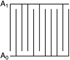
Figure 4: The extended tendrils used in the proof of the lower bound, in the special case where $d=2$. Each tendril has length $1-\varepsilon$ and joins up with either the top $A_{1}$ or bottom $A_{0}$ but not both.

Now we define extended tendrils that are joined to the top or bottom of the cube (but not both). See Figure 4. If

$$T_{j}=\bigl{\{}(s_{1}\varepsilon,s_{2}\varepsilon,\ldots,s_{d-1}\varepsilon,x_{d})\dvtx\varepsilon\leq x_{d}\leq 1-\varepsilon\bigr{\}}$$

is a tendril, define its extensions

$$T_{j,0} = \bigl{\{}(s_{1}\varepsilon,s_{2}\varepsilon,\ldots,s_{d-1}\varepsilon,x_{d})\dvtx 0\leq x_{d}\leq 1-\varepsilon\bigr{\}},$$

$$T_{1,j} = \bigl{\{}(s_{1}\varepsilon,s_{2}\varepsilon,\ldots,s_{d-1}\varepsilon,x_{d})\dvtx\varepsilon\leq x_{d}\leq 1\bigr{\}}.$$

Given $\omega\in\Omega=\{0,1\}^{q}$, let

$$S_{\omega}=A_{0}\cup A_{1}\cup\Biggl{(}\bigcup_{j=1}^{q}T_{j,\omega_{j}}\Biggr{)}$$

and

$$P_{\omega,X}=\frac{1}{4}\mu_{0}+\frac{1}{4}\mu_{1}+\frac{1}{2q(1-\varepsilon)}\sum_{j}\nu_{j,\omega_{j}},$$

where $\nu_{j,\omega_{j}}$ is one-dimensional Lebesgue measure on $T_{j,\omega_{j}}$. This $P_{\omega,X}$ is a probability measure supported on $S_{\omega}$.

Notice that $S_{\omega}$ consists of two connected components, namely,

$$U_{\omega}^{(1)}=A_{1}\cup\biggl{(}\bigcup_{j:\omega_{j}=1}T_{j,\omega_{j}}\biggr{)}\quad\mbox{and}\quad U_{\omega}^{(0)}=A_{0}\cup\biggl{(}\bigcup_{j:\omega_{j}=0}T_{j,\omega_{j}}\biggr{)}.$$

Let

$$f_{\omega}(x)=\frac{L\varepsilon}{8}I\bigl{(}x\in U_{\omega}^{(1)}\bigr{)}.$$

Finally, we define $P_{\omega}=P_{\omega,X}\times P_{\omega,Y|X}$ where $P_{\omega,Y|X}$ is a point mass at $f_{\omega}(X)$. Define $d^{2}(f,g)=\int(f(x)-g(x))^{2}\,d\mu(x)$.

We complete the proof with a series of claims.

Claim 1: For each $\omega\in\Omega$, $P_{\omega}\in{\cal P}_{n}$.

Proof: Let

$$\sigma=\biggl{(}\frac{1}{m}\biggr{)}^{{1}/({d(1+\gamma)})}$$

and let

$$\frac{3}{2+\xi}\frac{\log m}{m^{{1}/({1+\gamma})}}\leq\alpha\leq\sqrt{\frac{m^{{\gamma}/({1+\gamma})}}{\log m}}.$$ (21)

It follows that (C2) and (C3) hold. We must verify (C1). If $x$ and $y$ are in the same connected component, then $|f_{\omega}(x)-f_{\omega}(y)|=0$. Now let $x$ and $y$ be in different components, that is, $x\in U_{\omega}^{(1)},y\in U_{\omega}^{(0)}$. Let us choose $x$ and $y$ as close as possible in Euclidean distance; hence $\|x-y\|=\varepsilon$. Let $\gamma$ be any path connecting $x$ to $y$. Since $x$ and $y$ lie on different components, there exists a subset $\gamma_{0}$ of $\gamma$ of length at least $\varepsilon$ on which $P_{\omega}$ puts zero mass. By assumption (C3), $\sigma\leq\varepsilon/(4C_{0})$ and hence $P_{X,\sigma}$ puts zero mass on the portion of $\gamma_{0}$ that is at least $C_{0}\sigma$ away from the support of $P_{\omega}$. This has length at least $\varepsilon-2C_{0}\sigma\geq\varepsilon/2$. Since $p_{X,\sigma}(x)=0$ on a portion of $\gamma_{0}$,

$$D_{P,\alpha,\sigma}(x,y)\geq\frac{\varepsilon}{2}=\frac{\|x-y\|}{2}.$$

Hence, $\|x-y\|\leq 2D_{P,\alpha,\sigma}(x,y)$. Then

$$\frac{|f_{\omega}(x)-f_{\omega}(y)|}{D_{P,\alpha,\sigma}(x,y)}\leq\frac{2|f_{\omega}(x)-f_{\omega}(y)|}{\|x-y\|},$$

and the latter is maximized by finding two points $x$ and $y$ as close together with nonzero numerator. In this case, $\|x-y\|=\varepsilon$ and $|f_{\omega}(x)-f_{\omega}(y)|=L\varepsilon/8$. Hence, $|f_{\omega}(x)-f_{\omega}(y)|\leq LD_{P,\alpha,\sigma}(x,y)$ as required. Now we show that each $P=P_{\omega}$ satisfies

$${\cal N}(P,\alpha,\sigma,\varepsilon)\leq\biggl{(}\frac{C}{\varepsilon}\biggr{)}^{\xi}$$

for all $\varepsilon\geq n^{-{1}/({2+\xi})}$. Cover the top $A_{1}$ and bottom $A_{0}$ of the cubes with Euclidean spheres of radius $\delta$. There are $O((1/\delta)^{d-1})$ such spheres. The $D_{P,\alpha,\sigma}$ radius of each sphere is at most $\delta e^{-\alpha K(0)/\sigma^{d}}$. Thus, these form an $\varepsilon$ covering as long as $\delta e^{-\alpha K(0)/\sigma^{d}}\leq\varepsilon$. Thus the covering number of the top and bottom is at most $2(1/\delta)^{d-1}\leq 2(1/(e^{\alpha K(0)/\sigma^{d}}\varepsilon))^{d-1}$. Now cover the tendris with one-dimensional segments of length $\delta$. The $D_{P,\alpha,\sigma}$ radius of each segment is at most $\delta e^{-\alpha/\sigma^{d}}$. Thus, these form an $\varepsilon$ covering as long as $\delta e^{-\alpha K(0)/\sigma^{d}}\leq\varepsilon$. Thus the covering number of the tendrils is at most $q/\delta=n/\delta\leq n/(\varepsilon e^{\alpha K(0)/\sigma^{d}})$. Thus we can cover the support with

$$N(\varepsilon)\leq 2\biggl{(}\frac{1}{e^{\alpha K(0)/\sigma^{d}}\varepsilon}\biggr{)}^{d-1}+\frac{n}{\varepsilon e^{\alpha K(0)/\sigma^{d}}}$$

balls of size $\varepsilon$. It follows from (21) that $N(\varepsilon)\leq(1/\varepsilon)^{\xi}$ for $\varepsilon\geq n^{-{1}/({2+\xi})}$ as required.

Claim 2: For any $\omega$, and any $g\geq 0$, $\int g(x)\,dP_{\omega}(x)\geq\frac{1}{2}\int g(x)\,d\mu(x)$.

Proof: We have

$$\int_{S_{\omega}}g\,dP_{\omega} \geq \int_{C}g\,dP_{\omega}=\frac{1}{4}\int_{A_{0}}g\,d\mu_{0}+\frac{1}{4}\int_{A_{1}}g\,d\mu_{1}+\frac{\sum_{j}\int_{T_{j}}g\,d\nu_{j,\omega}}{2q(1-\varepsilon)}$$

$$= \frac{1}{4}\int_{A_{0}}g\,d\mu_{0}+\frac{1}{4}\int_{A_{1}}g\,d\mu_{1}$$

$${}+\frac{(({1-2\varepsilon})\sum_{j}\int_{T_{j}}g\,d\nu_{j})/({1-\varepsilon})}{2q(1-2\varepsilon)}\times\frac{{1}/{2}+q(1-2\varepsilon)}{{1}/{2}+q(1-\varepsilon)}$$

$$\geq \frac{1}{2}\biggl{(}\frac{1}{4}\int_{A_{0}}g\,d\mu_{0}+\frac{1}{4}\int_{A_{1}}gd\mu_{1}+\frac{\sum_{j}\int_{T_{j}}g\,d\nu_{j}}{2q(1-2\varepsilon)}\biggr{)}=\frac{1}{2}\int g\,d\mu.$$

Claim 3: For any $\omega,\nu\in\Omega$,

$$d^{2}(f_{\omega},f_{\nu})=\frac{\rho(\omega,\nu)L^{2}\varepsilon^{2}(1-2\varepsilon)}{2q(1-2\varepsilon)}.$$

Proof: This follows from direct calculation.

Claim 4: If $\rho(\omega,\nu)=1$, then $\|P_{\omega}^{n}\wedge P_{\nu}^{n}\|\geq 1/(16e)$.

Proof: Suppose that $\rho(\omega,\nu)=1$. $P_{\omega}$ and $P_{\nu}$ are the same everywhere except $T_{j,0}\cup T_{j,1}$, where $j$ is the index where $\omega$ and $\nu$ differ (assume $\omega_{j}=0$ and $\nu_{j}=1$). Define $A=T_{j,0}\times\{0\}$ and $B=T_{j,1}\times\{L\varepsilon\}$. Note that $A\cap B=\varnothing$. So,

$$P_{\omega}(T_{j,0}\cup T_{j,1})=P_{\omega}(A)=P_{\nu}(T_{j,0}\cup T_{j,1})=P_{\nu}(B)=\frac{1-\varepsilon}{2q(1-\varepsilon)}$$

and

$$\mathsf{TV}(P_{\omega},P_{\nu}) = \bigl{|}P_{\omega}(A)-P_{\nu}(A)\bigr{|}=\bigl{|}P_{\omega}(B)-P_{\nu}(B)\bigr{|}$$

$$= \frac{1-\varepsilon}{2q(1-\varepsilon)}=\frac{1}{2q}=\frac{\varepsilon^{d-1}}{2}.$$

Thus,

$$\bigl{\|}P_{\omega}^{n}\land P_{\nu}^{n}\bigr{\|}\geq\tfrac{1}{8}\bigl{(}1-\mathsf{TV}(P_{\omega},P_{\nu})\bigr{)}^{2n}\geq\tfrac{1}{8}\bigl{(}1-\varepsilon^{d-1}/2\bigr{)}^{2n}.$$

Since $\varepsilon=n^{-{1}/({d-1})}$, this implies that

$$\bigl{\|}P_{\omega}^{n}\land P_{\nu}^{n}\bigr{\|}\geq\frac{1}{8}\biggl{(}1-\frac{1}{2n}\biggr{)}^{2n}\geq\frac{1}{16e}$$

for all large $n$.

Completion of the proof. Recall that $\varepsilon=n^{-{1}/({d-1})}$. Combining Assouad’s lemma (see Lemma 3 in the supplement) with the above claims, we have

$$R_{S} = \inf_{\widehat{f}\in{\cal S}_{n}}\sup_{P\in{\cal P}_{n,\xi}}R_{P}(\widehat{f})\geq\inf_{\widehat{f}\in{\cal S}_{n}}\sup_{P\in{\cal P}_{\Omega}}R_{P}(\widehat{f})\geq\frac{1}{2}\inf_{\widehat{f}}\max_{\omega\in\Omega}\mathbb{E}_{\omega}\bigl{[}d^{2}(f_{\omega},\widehat{f})\bigr{]}$$

$$\geq \frac{q}{16}\times\frac{(L/8)^{2}\varepsilon^{2}(1-2\varepsilon)}{2q(1-2\varepsilon)}\times\frac{1}{16e}=C\frac{q\varepsilon^{2}(1-2\varepsilon)}{2q(1-2\varepsilon)}$$

$$\geq C\varepsilon^{2}=Cn^{-{2}/({d-1})}.$$

5.3 Semisupervised upper bound

Now we state the upper bound for this class.

Theorem 5.2

Let $h=(ne^{2(2-\xi)})^{-{1}/({2+\xi})}$. Then

$$\sup_{P\in{\cal P}_{n}}R(\widehat{f}_{h,\alpha,\sigma})\leq\biggl{(}\frac{C}{n}\biggr{)}^{{2}/({2+\xi})}.$$ (22)

This follows from (C2), (C3) and Corollary 4.2.

5.4 Comparison of lower and upper bound

Combining the last two theorems we have:

Corollary 5.3

Under the conditions of the previous theorem, and assuming that $d>\xi+3$,

$$\frac{R_{SS}}{R_{S}}\preceq\biggl{(}\frac{1}{n}\biggr{)}^{{2(d-3-\xi)}/({(2+\xi)(d-1)})}\to 0$$ (23)

as $n\to\infty$.

This establishes the effectiveness of semi-supervised inference in the minimax sense.

6 Adaptive semisupervised inference

We have established a bound on the risk of the density-sensitive semisupervised kernel estimator. The bound is achieved by using an estimate $\widehat{D}_{\alpha,\sigma}$ of the density-sensitive distance. However, this requires knowing the density-sensitive parameter $\alpha$, along with other parameters. It is critical to choose $\alpha$ (and $h$) appropriately, otherwise we might incur a large error if the semisupervised assumption does not hold, or holds with a different density sensitivity value $\alpha$. We consider two methods for choosing the parameters.

The following result shows that we can adapt to the correct degree of semisupervisedness if cross-validation is used to select the appropriate $\alpha,\sigma$ and $h$. This implies that the estimator gracefully degrades to a supervised learner if the semisupervised assumption (sensitivity of regression function to marginal density) does not hold ($\alpha=0$).

For any $f$, define the risk $R(f)=\mathbb{E}[(f(X)-Y)^{2}]$ and the excess risk ${\cal E}(f)=R(f)-R(f^{*})=\mathbb{E}[(f(X)-f^{*}(X))^{2}]$ where $f^{*}$ is the true regression function. Let ${\cal H}$ be a finite set of bandwidths, let ${\cal A}$ be a finite set of values for $\alpha$ and let $\Sigma$ be a finite set of values for $\sigma$. Let $\theta=(h,\alpha,\sigma)$, $\Theta={\cal H}\times{\cal A}\times\Sigma$ and $J=|\Theta|$.

Divide the data into training data $T$ and validation data $V$. For notational simplicity, let both sets have size $n$. Let ${\cal F}=\{\widehat{f}^{T}_{\theta}\}_{\theta\in\Theta}$ denote the semisupervised kernel estimators trained on data $T$ using $\theta\in\Theta$. For each $\widehat{f}_{\theta}^{T}\in{\cal F}$ let

$$\widehat{R}^{V}\bigl{(}\widehat{f}^{T}_{\theta}\bigr{)}=\frac{1}{n}\sum^{n}_{i=1}\bigl{(}\widehat{f}^{T}_{\theta}(X_{i})-Y_{i}\bigr{)}^{2},$$

where the sum is over $V$. Let $Y_{i}=f(X_{i})+\varepsilon_{i}$ with $\varepsilon_{i}\stackrel{{\scriptstyle\mathrm{i.i.d.}}}{{\sim}}{\cal N}(0,\sigma^{2})$. Also, we assume that $|f(x)|,|\widehat{f}^{T}_{\theta}(x)|\leq M$, where $M>0$ is a constant.

Theorem 6.1

Let ${\cal F}=\{\widehat{f}^{T}_{\theta}\}_{\theta\in\Theta}$ denote the semisupervised kernel estimators trained on data $T$ using $\theta\in\Theta$. Use validation data $V$ to pick

$$\widehat{\theta}=\mathop{\arg\min}_{\theta\in\Theta}\widehat{R}^{V}\bigl{(}\widehat{f}^{T}_{\theta}\bigr{)}$$

and define the corresponding estimator $\widehat{f}=\widehat{f}_{\widehat{\theta}}$. Then, for every $0<\delta<1$,

$$\mathbb{E}\bigl{[}{\cal E}(\widehat{f}_{\theta})\bigr{]}\leq\frac{1}{1-a}\biggl{[}\min_{\theta\in\Theta}\mathbb{E}\bigl{[}{\cal E}(\widehat{f}_{\theta})\bigr{]}+\frac{\log(J)/\delta)}{nt}\biggr{]}+4\delta M^{2},$$ (24)

where $0<a<1$ and $0<t<15/(38(M^{2}+\sigma^{2}))$ are constants. $\mathbb{E}$ denotes expectation over everything that is random.

First, we derive a general concentration of $\widehat{\cal E}(f)$ around ${\cal E}(f)$ where $\widehat{\cal E}(f)=\widehat{R}(f)-\widehat{R}(f^{*})=-\frac{1}{n}\sum^{n}_{i=1}U_{i}$ and $U_{i}=-(Y_{i}-f(X_{i}))^{2}+(Y_{i}-f^{*}(X_{i}))^{2}$.

If the variables $U_{i}$ satisfy the following moment condition:

$$\mathbb{E}\bigl{[}\bigl{|}U_{i}-\mathbb{E}[U_{i}]\bigr{|}^{k}\bigr{]}\leq\frac{\mathsf{Var}(U_{i})}{2}k!r^{k-2}$$

for some $r>0$, then the Craig–Bernstein (CB) inequality [Craig (1933)] states that with probability $>1-\delta$,

$$\frac{1}{n}\sum^{n}_{i=1}\bigl{(}U_{i}-\mathbb{E}[U_{i}]\bigr{)}\leq\frac{\log(1/\delta)}{nt}+\frac{t\operatorname{\mathsf{Var}}(U_{i})}{2(1-c)}$$

for $0\leq tr\leq c<1$. The moment conditions are satisfied by bounded random variables as well as Gaussian random variables; see, for example, Haupt and Nowak (2006).

To apply this inequality, we first show that $\mathsf{Var}(U_{i})\leq 4(M^{2}+\sigma^{2}){\cal E}(f)$ since $Y_{i}=f(X_{i})+\varepsilon_{i}$ with $\varepsilon_{i}\stackrel{{\scriptstyle\mathrm{i.i.d.}}}{{\sim}}{\cal N}(0,\sigma^{2})$. Also, we assume that $|f(x)|$, $|\widehat{f}(x)|\leq M$, where $M>0$ is a constant.

$$\mathsf{Var}(U_{i}) \leq \mathbb{E}\bigl{[}U_{i}^{2}\bigr{]}=\mathbb{E}\bigl{[}\bigl{(}-\bigl{(}Y_{i}-f(X_{i})\bigr{)}^{2}+\bigl{(}Y_{i}-f^{*}(X_{i})\bigr{)}^{2}\bigr{)}^{2}\bigr{]}$$

$$= \mathbb{E}\bigl{[}\bigl{(}-\bigl{(}f^{*}(X_{i})+\varepsilon_{i}-f(X_{i})\bigr{)}^{2}+(\varepsilon_{i})^{2}\bigr{)}^{2}\bigr{]}$$

$$= \mathbb{E}\bigl{[}\bigl{(}-\bigl{(}f^{*}(X_{i})-f(X_{i})\bigr{)}^{2}-2\varepsilon_{i}\bigl{(}f^{*}(X_{i})-f(X_{i})\bigr{)}\bigr{)}^{2}\bigr{]}$$

$$\leq 4M^{2}{\cal E}(f)+4\sigma^{2}{\cal E}(f)=4\bigl{(}M^{2}+\sigma^{2}\bigr{)}{\cal E}(f).$$

Therefore using the CB inequality we get, with probability $>1-\delta$,

$${\cal E}(f)-\widehat{\cal E}(f)\leq\frac{\log(1/\delta)}{nt}+\frac{t2(M^{2}+\sigma^{2}){\cal E}(f)}{(1-c)}.$$

Now set $c=tr=8t(M^{2}+\sigma^{2})/15$ and let $t<15/(38(M^{2}+\sigma^{2}))$. With this choice, $c<1$ and define

$$a=\frac{t2(M^{2}+\sigma^{2})}{(1-c)}<1.$$

Then, using $a$ and rearranging terms, with probability $>1-\delta$,

$$(1-a){\cal E}(f)-\widehat{\cal E}(f)\leq\frac{\log(1/\delta)}{nt},$$

where $t<15/(38(M^{2}+\sigma^{2}))$.

Then, using the previous concentration result, and taking union bound over all $f\in{\cal F}$, we have with probability $>1-\delta$,

$${\cal E}(f)\leq\frac{1}{1-a}\biggl{[}\widehat{\cal E}^{V}(f)+\frac{\log(J/\delta)}{nt}\biggr{]}.$$

Now,

$${\cal E}(\widehat{f}_{\widehat{\theta}}) = R(\widehat{f}_{\widehat{\theta}})-R\bigl{(}f^{*}\bigr{)}$$

$$\leq \frac{1}{1-a}\biggl{[}\widehat{R}^{V}(\widehat{f}_{\widehat{\theta}})-\widehat{R}^{V}\bigl{(}f^{*}\bigr{)}+\frac{\log(J/\delta)}{nt}\biggr{]}$$

$$\leq \frac{1}{1-a}\biggl{[}\widehat{R}^{V}(f)-\widehat{R}^{V}\bigl{(}f^{*}\bigr{)}+\frac{\log(J/\delta)}{nt}\biggr{]}.$$

Taking expectation with respect to validation dataset,

$$\mathbb{E}_{V}\bigl{[}{\cal E}(\widehat{f}_{\widehat{\theta}})\bigr{]}\leq\frac{1}{1-a}\biggl{[}R(f)-R\bigl{(}f^{*}\bigr{)}+\frac{\log(J/\delta)}{nt}\biggr{]}+4\delta M^{2}.$$

Now taking expectation with respect to training dataset,

$$\mathbb{E}_{\mathrm{TV}}\bigl{[}{\cal E}(\widehat{f}_{\widehat{\theta}})\bigr{]}\leq\frac{1}{1-a}\biggl{[}\mathbb{E}_{T}\bigl{[}R(f)-R\bigl{(}f^{*}\bigr{)}\bigr{]}+\frac{\log(J/\delta)}{nt}\biggr{]}+4\delta M^{2}.$$

Since this holds for all $f\in{\cal F}$, we get

$$\mathbb{E}_{\mathrm{TV}}\bigl{[}{\cal E}(\widehat{f}_{\widehat{\theta}})\bigr{]}\leq\frac{1}{1-a}\biggl{[}\min_{f\in{\cal F}}\mathbb{E}_{T}\bigl{[}{\cal E}(f)\bigr{]}+\frac{\log(J/\delta)}{nt}\biggr{]}+4\delta M^{2}.$$

The result follows.

In practice, both $\Theta$ may be taken to be of size $n^{a}$ for some $a>0$. Then we can approximate the optimal $h,\sigma$ and $\alpha$ with sufficient accuracy to achieve the optimal rate. Setting $\delta=1/(4M^{2}n)$, we then see that the penalty for adaptation is $\frac{\log(J/\delta)}{nt}+\delta M=O(\log n/n)$ and hence introduces only a logarithmic term.

Cross-validation is not the only way to adapt. For example, the adaptive method in Kpotufe (2011) can also be used here.

7 Simulation results

In this section we describe the results of a series of numerical experiments on a simulated data set to demonstrate the effect of using the exponential version of the density sensitive metric for small, labeled sample sizes. For the marginal distribution of $X$, we used a slightly modified version of the swiss roll distribution used in Culp (2011b). Figure 5 shows a sample from this distribution, where the point size represents the response $Y$. We repeatedly sampled $N=400$ points from this distribution, and computed the mean squared error of the kernel regression estimator using a set of values for $\alpha$ and for labeled sample size ranging from $n=5$ to $n=320$. We used the approximation method described in the supplement [see equation (10)] with the number of nearest neighbors used set to $k=20$.

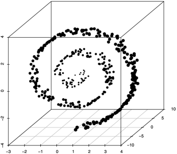
Figure 5: The swiss roll data set. Point size represents regression function.

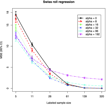
Figure 6: MSE of kernel regression on the swiss roll data set for a range of labeled sample sizes using different values of $\alpha$.

Figure 6 shows the average results after $300$ repetitions of this procedure with error bars indicating a $95\%$ confidence interval. As expected, we observe that for small labeled sample sizes, increasing $\alpha$ can decrease the error. But as the labeled sample size increases, using the density sensitive metric becomes decreasingly beneficial, and can even hurt.

8 Discussion

Semisupervised methods are very powerful, but like all methods, they only work under certain conditions. We have shown that, under certain conditions, semisupervised methods provably outperform supervised methods. In particular, the advantage of semisupervised methods is mainly when the distribution $P_{X}$ of $X$ is concentrated near a low-dimensional set rather than when $P_{X}$ is smooth.

We introduced a family of estimators indexed by a parameter $\alpha$. This parameter controls the strength of the semi-supervised assumption. The behavior of the semi-supervised method depends critically on $\alpha$. Finally, we showed that cross-validation can be used to automatically adapt to $\alpha$ so that $\alpha$ does not need to be known. Hence, our method takes advantage of the unlabeled data when the semi-supervised assumption holds, but does not add extra bias when the assumption fails. Our simulations confirm that our proposed estimator has good risk when the semi-supervised smoothness holds.

The analysis in this paper can be extended in several ways. First, it is possible to use other density sensitive metrics such as the diffusion distance [Lee and Wasserman (2008)]. Second, we defined a method to estimate the density sensitive metric that works under broader conditions than the two existing methods due to Sajama and Orlitsky (2005) and Bijral, Ratliff and Srebro (2011). We suspect that faster methods can be developed. Finally, other estimators besides kernel estimators can be used. We will report on these extensions elsewhere.

Supplement to “Density-sensitive semisupervised inference”
[doi]10.1214/13-AOS1092SUPP .pdf aos1092_supp.pdf Contains technical details, proofs and extensions.

References

- Azizyan, Singh and Wasserman (2013) {bmisc}[author] \bauthor\bsnmAzizyan, \bfnmMartin\binitsM., \bauthor\bsnmSingh, \bfnmAarti\binitsA. and \bauthor\bsnmWasserman, \bfnmLarry\binitsL. (\byear2013). \bhowpublishedSupplement to “Density-sensitive semisupervised inference.” DOI:\doiurl10.1214/13-AOS1092SUPP. \bptokimsref \endbibitem
- Belkin and Niyogi (2004) {barticle}[author] \bauthor\bsnmBelkin, \bfnmM.\binitsM. and \bauthor\bsnmNiyogi, \bfnmP.\binitsP. (\byear2004). \btitleSemi-supervised learning on Riemannian manifolds. \bjournalMachine Learning \bvolume56 \bpages209–239. \bptokimsref \endbibitem
- Ben-David, Lu and Pal (2008) {bmisc}[author] \bauthor\bsnmBen-David, \bfnmS.\binitsS., \bauthor\bsnmLu, \bfnmT.\binitsT. and \bauthor\bsnmPal, \bfnmD.\binitsD. (\byear2008). \bhowpublishedDoes unlabeled data provably help? Worst-case analysis of the sample complexity of semi-supervised learning. In 21st Annual Conference on Learning Theory (COLT). Available at http://www.informatik.uni-trier.de/~ley/db/conf/colt/colt2008.html. \bptokimsref \endbibitem
- Bijral, Ratliff and Srebro (2011) {bmisc}[author] \bauthor\bsnmBijral, \bfnmAvleen\binitsA., \bauthor\bsnmRatliff, \bfnmNathan\binitsN. and \bauthor\bsnmSrebro, \bfnmNathan\binitsN. (\byear2011). \bhowpublishedSemi-supervised learning with density based distances. In 27th Conference on Uncertainty in Artificial Intelligence. Available at http://auai.org/uai2011/accepted.html. \bptokimsref \endbibitem
- Bousquet, Chapelle and Hein (2004) {binproceedings}[author] \bauthor\bsnmBousquet, \bfnmO.\binitsO., \bauthor\bsnmChapelle, \bfnmO.\binitsO. and \bauthor\bsnmHein, \bfnmM.\binitsM. (\byear2004). \btitleMeasure based regularization. In \bbooktitleAdvances in Neural Information Processing Systems \bvolume16. \bpublisherMIT Press, \blocationCambridge, MA. \bptokimsref \endbibitem
- Castelli and Cover (1995) {barticle}[author] \bauthor\bsnmCastelli, \bfnmVittorio\binitsV. and \bauthor\bsnmCover, \bfnmThomas M.\binitsT. M. (\byear1995). \btitleOn the exponential value of labeled samples. \bjournalPattern Recognition Letters \bvolume16 \bpages105–111. \bptokimsref \endbibitem
- Castelli and Cover (1996) {barticle}[mr] \bauthor\bsnmCastelli, \bfnmVittorio\binitsV. and \bauthor\bsnmCover, \bfnmThomas M.\binitsT. M. (\byear1996). \btitleThe relative value of labeled and unlabeled samples in pattern recognition with an unknown mixing parameter. \bjournalIEEE Trans. Inform. Theory \bvolume42 \bpages2102–2117. \biddoi=10.1109/18.556600, issn=0018-9448, mr=1447517 \bptokimsref \endbibitem
- Craig (1933) {barticle}[auto:STB—2013/04/11—08:11:48] \bauthor\bsnmCraig, \bfnmCecil C.\binitsC. C. (\byear1933). \btitleOn the Tchebychef inequality of Bernstein. \bjournalAnn. Math. Statist. \bvolume4 \bpages94–102. \bptokimsref \endbibitem
- Culp (2011a) {barticle}[mr] \bauthor\bsnmCulp, \bfnmMark\binitsM. (\byear2011a). \btitleOn propagated scoring for semisupervised additive models. \bjournalJ. Amer. Statist. Assoc. \bvolume106 \bpages248–259. \biddoi=10.1198/jasa.2011.tm09316, issn=0162-1459, mr=2816718 \bptokimsref \endbibitem
- Culp (2011b) {barticle}[author] \bauthor\bsnmCulp, \bfnmMark\binitsM. (\byear2011b). \btitlespa: Semi-supervised semi-parametric graph-based estimation in R. \bjournalJournal of Statistical Software \bvolume40 \bpages1–29. \bptokimsref \endbibitem
- Culp and Michailidis (2008) {barticle}[mr] \bauthor\bsnmCulp, \bfnmMark\binitsM. and \bauthor\bsnmMichailidis, \bfnmGeorge\binitsG. (\byear2008). \btitleAn iterative algorithm for extending learners to a semi-supervised setting. \bjournalJ. Comput. Graph. Statist. \bvolume17 \bpages545–571. \biddoi=10.1198/106186008X344748, issn=1061-8600, mr=2451341 \bptokimsref \endbibitem
- Györfi et al. (2002) {bbook}[mr] \bauthor\bsnmGyörfi, \bfnmLászló\binitsL., \bauthor\bsnmKohler, \bfnmMichael\binitsM., \bauthor\bsnmKrzyżak, \bfnmAdam\binitsA. and \bauthor\bsnmWalk, \bfnmHarro\binitsH. (\byear2002). \btitleA Distribution-Free Theory of Nonparametric Regression. \bpublisherSpringer, \blocationNew York. \biddoi=10.1007/b97848, mr=1920390 \bptokimsref \endbibitem
- Haupt and Nowak (2006) {barticle}[mr] \bauthor\bsnmHaupt, \bfnmJarvis\binitsJ. and \bauthor\bsnmNowak, \bfnmRobert\binitsR. (\byear2006). \btitleSignal reconstruction from noisy random projections. \bjournalIEEE Trans. Inform. Theory \bvolume52 \bpages4036–4048. \biddoi=10.1109/TIT.2006.880031, issn=0018-9448, mr=2298532 \bptokimsref \endbibitem
- Kpotufe (2011) {bincollection}[author] \bauthor\bsnmKpotufe, \bfnmSamory\binitsS. (\byear2011). \btitle-NN regression adapts to local intrinsic dimension. In \bbooktitleAdvances in Neural Information Processing Systems \bvolume24 \bpages729–737. \bpublisherMIT Press, \blocationCambridge, MA. \bptokimsref \endbibitem
- Lafferty and Wasserman (2007) {binproceedings}[author] \bauthor\bsnmLafferty, \bfnmJohn\binitsJ. and \bauthor\bsnmWasserman, \bfnmLarry\binitsL. (\byear2007). \btitleStatistical analysis of semi-supervised regression. In \bbooktitleAdvances in Neural Information Processing Systems \bvolume20 \bpages801–808. \bpublisherMIT Press, \blocationCambridge, MA. \bptokimsref \endbibitem
- Lee and Wasserman (2008) {bmisc}[author] \bauthor\bsnmLee, \bfnmA. B.\binitsA. B. and \bauthor\bsnmWasserman, \bfnmL.\binitsL. (\byear2008). \bhowpublishedSpectral connectivity analysis. Preprint. Available at arXiv:\arxivurl0811.0121. \bptokimsref \endbibitem
- Liang, Mukherjee and West (2007) {barticle}[mr] \bauthor\bsnmLiang, \bfnmFeng\binitsF., \bauthor\bsnmMukherjee, \bfnmSayan\binitsS. and \bauthor\bsnmWest, \bfnmMike\binitsM. (\byear2007). \btitleThe use of unlabeled data in predictive modeling. \bjournalStatist. Sci. \bvolume22 \bpages189–205. \biddoi=10.1214/088342307000000032, issn=0883-4237, mr=2408958 \bptokimsref \endbibitem
- Nadler, Srebro and Zhou (2009) {binproceedings}[author] \bauthor\bsnmNadler, \bfnmBoaz\binitsB., \bauthor\bsnmSrebro, \bfnmNathan\binitsN. and \bauthor\bsnmZhou, \bfnmXueyuan\binitsX. (\byear2009). \btitleStatistical analysis of semi-supervised learning: The limit of infinite unlabelled data. In \bbooktitleAdvances in Neural Information Processing Systems \bvolume22 \bpages1330–1338. \bpublisherMIT Press, \blocationCambridge, MA. \bptokimsref \endbibitem
- Niyogi (2008) {bmisc}[author] \bauthor\bsnmNiyogi, \bfnmP.\binitsP. (\byear2008). \bhowpublishedManifold regularization and semi-supervised learning: Some theoretical analyses. Technical Report TR-2008-01, Computer Science Dept., Univ. Chicago. Available at http://people.cs.uchicago.edu/~niyogi/papersps/ssminimax2.pdf. \bptokimsref \endbibitem
- Ratsaby and Venkatesh (1995) {binproceedings}[author] \bauthor\bsnmRatsaby, \bfnmJ.\binitsJ. and \bauthor\bsnmVenkatesh, \bfnmS. S.\binitsS. S. (\byear1995). \btitleLearning from a mixture of labeled and unlabeled examples with parametric side information. In \bbooktitleProceedings of the Eighth Annual Conference on Computational Learning Theory \bpages412–417. \bpublisherACM, \blocationNew York. \bptokimsref \endbibitem
- Rigollet (2007) {barticle}[mr] \bauthor\bsnmRigollet, \bfnmPhilippe\binitsP. (\byear2007). \btitleGeneralized error bounds in semi-supervised classification under the cluster assumption. \bjournalJ. Mach. Learn. Res. \bvolume8 \bpages1369–1392. \bidissn=1532-4435, mr=2332435 \bptokimsref \endbibitem
- Sajama and Orlitsky (2005) {binproceedings}[author] \bauthor\bsnmSajama and \bauthor\bsnmOrlitsky, \bfnmAlon\binitsA. (\byear2005). \btitleEstimating and computing density based distance metrics. In \bbooktitleProceedings of the 22nd International Conference on Machine Learning. ICML 2005 \bpages760–767. \bpublisherACM, \blocationNew York. \bptokimsref \endbibitem
- Singh, Nowak and Zhu (2008) {bmisc}[author] \bauthor\bsnmSingh, \bfnmAarti\binitsA., \bauthor\bsnmNowak, \bfnmR. D.\binitsR. D. and \bauthor\bsnmZhu, \bfnmX.\binitsX. (\byear2008). \bhowpublishedUnlabeled data: Now it helps, now it doesn’t. Technical report, ECE Dept., Univ. Wisconsin–Madison. Available at http://www.cs.cmu.edu/~aarti/pubs/SSL_TR.pdf. \bptokimsref \endbibitem
- Sinha and Belkin (2009) {bincollection}[author] \bauthor\bsnmSinha, \bfnmKaushik\binitsK. and \bauthor\bsnmBelkin, \bfnmMikhail\binitsM. (\byear2009). \btitleSemi-supervised learning using sparse eigenfunction bases. In \bbooktitleAdvances in Neural Information Processing Systems \bvolume22 (\beditor\bfnmY.\binitsY. \bsnmBengio, \beditor\bfnmD.\binitsD. \bsnmSchuurmans, \beditor\bfnmJ.\binitsJ. \bsnmLafferty, \beditor\bfnmC. K. I.\binitsC. K. I. \bsnmWilliams and \beditor\bfnmA.\binitsA. \bsnmCulotta, eds.) \bpages1687–1695. \bpublisherMIT Press, \blocationCambridge, MA. \bptokimsref \endbibitem