Dynamical properties of the unitary Fermi gas:
collective modes and shock waves

Abstract

We discuss the unitary Fermi gas made of dilute and ultracold atoms with an infinite s-wave inter-atomic scattering length. First we introduce an efficient Thomas-Fermi-von Weizsacker density functional which describes accurately various static properties of the unitary Fermi gas trapped by an external potential. Then, the sound velocity and the collective frequencies of oscillations in a harmonic trap are derived from extended superfluid hydrodynamic equations which are the Euler-Lagrange equations of a Thomas-Fermi-von Weizsacker action functional. Finally, we show that this amazing Fermi gas supports supersonic and subsonic shock waves.

PACS numbers: 03.75.Ss, 05.30.Fk, 71.10.Ay, 67.85.Lm

1 Introduction

For interacting fermions at very low temperature, far below the Fermi temperature $T_{F}$, the effects of quantum statistics become very important [1]. When the densities of the two spin components are equal, and when the gas is dilute so that the range of the inter-atomic potential is much smaller than the inter-particle distance, then the interaction effects are described by only one parameter: the s-wave scattering length $a_{F}$ [1; 2]. The sign of $a_{F}$ determines the character of the gas. Fano-Feshbach resonances can be used to change the value and the sign of the scattering length, simply by tuning an external magnetic field. At resonance the scattering length $a_{F}$ diverges so that the gas displays a very peculiar character, being at the same time dilute and strongly interacting. In this regime all scales associated with interactions disappear from the problem and the energy of the system is expected to be proportional to that of a non interacting fermions system. This is called the unitary regime [2].

Recently it has been remarked [3] that the unitary Fermi gas at zero temperature can be described by the density functional theory. Indeed, different theoretical groups have proposed various density functionals. For example, Bulgac and Yu have introduced a superfluid density functional based on a Bogoliubov-de Gennes approach to superfluid fermions [4; 5]. Papenbrock and Bhattacharyya [6] have instead proposed a Kohn-Sham density functional with an effective mass to take into account nonlocality effects. Here we adopt the extended Thomas-Fermi (ETF) functional of the unitary Fermi gas we have proposed few years ago [7; 8] which is a functional of the fermions number density $n({\bf r})$ and of its gradient. The total energy in the ETF functional contains a term proportional to the kinetic energy of a uniform non interacting gas of fermions, plus a gradient correction of the von-Weizsacker form $\lambda\hbar^{2}/(8m)(\nabla n/n)^{2}$ [9]. This approach has been adopted for studying the quantum hydrodynamics of electrons by March and Tosi [10], and by Zaremba and Tso [11]. In the context of the BCS-BEC crossover, the gradient term is quite standard [12; 13; 14; 15; 16; 17; 18; 19]. The main advantage of taking such a functional is the fact that, as it depends only on a single function of the coordinates, there is no limitation on the number of particles $N$ which it can treat. Other functionals, based on single-particle orbitals, require self-consistent calculations with a numerical load increasing with $N$.

In this paper we review the last achievements obtained by using our ETF density functional and its time-dependent version [7; 8]. Indeed we have successfully applied this density functional to investigate density profiles [7; 8; 20], collective excitations [20], Josephson effect [21] and shock waves [22] of the unitary Fermi gas. In addition, the collective modes of our EFT density functional have been used to study the low-temperature thermodynamics of the unitary Fermi gas (superfluid fraction, first sound and second sound) [23] and also the viscosity-entropy ratio of the unitary Fermi gas from zero-temperature elementary excitations [24].

2 BCS-BEC crossover and the unitarity limit

In 2002 the BCS-BEC crossover has been observed [25] with ultracold gases made of fermionic alkali-metal atoms. This crossover is obtained by changing with a Feshbach resonance the s-wave scattering length $a_{F}$ of the inter-atomic potential: if $a_{F}\to 0^{-}$ one gets the BCS regime of weakly-interacting Cooper pairs, if $a_{F}\to\pm\infty$ there is the unitarity limit of strongly-interacting Cooper pairs, and if $a_{F}\to 0^{+}$ one reaches the BEC regime of bosonic dimers. The many-body Hamiltonian of a two-spin-component Fermi system can be written as

$${\hat{H}}=\sum_{i=1}^{N_{\uparrow}}\left({{\hat{p}}_{i}^{2}\over 2m}+U({\bf r}_{i})\right)+\sum_{j=1}^{N_{\downarrow}}\left({{\hat{p}}_{j}^{2}\over 2m}+U({\bf r}_{j})\right)+\sum_{i,j}V({\bf r}_{i}-{\bf r}_{j})\;,$$ (1)

where $U({\bf r})$ is the external confining potential and $V({\bf r})$ is the inter-atomic potential. Here we consider $N_{\uparrow}=N_{\downarrow}$. The inter-atomic potential of a dilute gas can be modelled by a square well potential:

$$V(r)=\left\{\begin{array}[]{cc}-V_{0}&\mbox{ for }r<r_{0}\\ 0&\mbox{ for }r>r_{0}\\ \end{array}\right.$$ (2)

where $r_{0}$ is the effective radius. By varying the depth $V_{0}$ of the potential one changes the s-wave scattering length

$$a_{F}=r_{0}\left(1-{tan(r_{0}\sqrt{mV_{0}}/\hbar)\over r_{0}\sqrt{mV_{0}}/\hbar}\right)\;.$$ (3)

The crossover from a BCS superfluid ($a_{F}<0$) to a BEC of molecular pairs ($a_{F}>0$) has been investigated experimentally [2], and it has been shown that the unitary Fermi gas ($|a_{F}|=\infty$) exists and is meta-stable. In few words, the unitarity regime of a dilute Fermi gas is characterized by

$$r_{0}\ll n^{-1/3}\ll|a_{F}|\;.$$ (4)

Under these conditions the Fermi gas is called unitary Fermi gas. Ideally, the unitarity limit corresponds to

$$r_{0}=0\quad\quad\mbox{and}\quad\quad a_{F}=\pm\infty\;.$$ (5)

The detection of quantized vortices under rotation [26] has clarified that the unitary Fermi gas is superfluid.

The only length characterizing the uniform unitary Fermi gas is the average distance between particles $d=n^{-1/3}$. In this case, from simple dimensional arguments, the ground-state energy per volume must be

$${E_{0}\over V}={\xi}{3\over 5}{\hbar^{2}\over 2m}(3\pi^{2})^{2/3}n^{5/3}={\xi}\ {3\over 5}\ \epsilon_{F}\ n\;,$$ (6)

with $\epsilon_{F}$ Fermi energy of the ideal gas, $n=N/V$ the total density, and $\xi$ a universal unknown parameter. Monte Carlo calculations and experimental data with dilute and ultracold atoms suggest [2] that ${\xi}\simeq 0.4$.

3 Extended Thomas-Fermi density functional

The Thomas-Fermi (TF) energy functional [2] of the unitary Fermi gas in an external potential $U({\bf r})$ is given by

$$E=\int d^{3}{\bf r}\ \Big{[}{\xi}{3\over 5}{\hbar^{2}\over 2m}(3\pi^{2})^{2/3}n^{5/3}({\bf r})+U({\bf r})\,n({\bf r})\Big{]}\ ,$$ (7)

with $n({\bf r})=n_{\uparrow}({\bf r})+n_{\downarrow}({\bf r})$ total local density. The total number of fermions is

$$N=\int d^{3}{\bf r}\ n({\bf r})\;.$$ (8)

By minimizing $E$ one finds

$${\xi}{\hbar^{2}\over 2m}(3\pi^{2})^{2/3}n^{2/3}({\bf r})+U({\bf r})=\bar{\mu}\;,$$ (9)

with $\bar{\mu}$ chemical potential of the non uniform system. The TF functional can be extended to cure the pathological TF behavior at the surface, namely the fact that the density goes to zero at a finite distance from the center of the cloud. We add to the energy density the term

$${\lambda}{\hbar^{2}\over 8m}{(\nabla n)^{2}\over n}={\lambda}{\hbar^{2}\over 2m}{(\nabla\sqrt{n})^{2}}\;.$$ (10)

Historically, this term was introduced by von Weizsäcker [9] to treat surface effects in nuclei. Here we consider ${\lambda}$ as a phenomenological parameter accounting for the increase of kinetic energy due the spatial variation of the density. The new energy functional, that is the extended Thomas-Fermi (ETF) functional of the unitary Fermi gas, reads

$$E=\int d^{3}{\bf r}\ \left[\lambda{\hbar^{2}\over 8m}{(\nabla n({\bf r}))^{2}\over n({\bf r})}+{\xi}{3\over 5}{\hbar^{2}\over 2m}(3\pi^{2})^{5/3}n({\bf r})^{5/3}+U({\bf r})\,n({\bf r})\right]\ \;.$$ (11)

By minimizing the ETF energy functional one gets:

$$\left[{\lambda}{\hbar^{2}\over 2m}\nabla^{2}+{\xi}{\hbar^{2}\over 2m}(3\pi^{2})^{2/3}n({\bf r})^{2/3}+U({\bf r})\right]\sqrt{n({\bf r})}=\bar{\mu}\ \sqrt{n({\bf r})}\;.$$ (12)

This is a sort of stationary 3D nonlinear Schrödinger equation. In recent papers [7; 8; 20; 23; 24] we have determined the parameters $\xi$ and $\lambda$ by fitting recent Monte Carlo results [27; 28; 29] for the energy of fermions confined in a spherical harmonic trap of frequency $\omega$ in this regime. The main conclusion is that the values

$$\xi=0.40\quad\quad\mbox{and}\quad\quad\lambda=1/4\;$$ (13)

fit quite well Monte Carlo data of the unitary Fermi gas. Having determined the parameters $\xi$ and $\lambda$, one can use our single-orbital density functional to calculate various properties of the trapped unitary Fermi gas. Ground-state energies and density profiles have been analyzed in Ref. [7; 20], showing a very good agreement with other theoretical aproaches [28; 4].

4 Generalized superfluid hydrodynamics

Here we analyze the effect of the gradient term on the dynamics of the superfluid unitary Fermi gas. At zero temperature the low-energy collective dynamics of this fermionic gas can be described by the superfluid equations of inviscid hydrodynamics [2]:

$${\partial n\over\partial t}+\nabla\cdot(n{\bf v})=0\;,$$ (14)

$$m{\partial\over\partial t}{\bf v}+\nabla\Big{[}{\xi}{\hbar^{2}\over 2m}(3\pi^{2}n)^{2/3}+U({\bf r})+{m\over 2}v^{2}\Big{]}=0\;,$$ (15)

where the velocity $\bf v$ is irrotational: $\nabla\wedge{\bf v}=0$, i.e.

$${\bf v}({\bf r},t)={\hbar\over 2m}\nabla\theta({\bf r},t)\;,$$ (16)

with $\theta({\bf r},t)$ the phase of the condensate wave function of Cooper pairs. It is straightforward to show that these equations are the Euler-Lagrange equations of the following TF action functional

$$A=\int dt\,d^{3}{\bf r}\left[{\hbar\over 2}{\dot{\theta}}\,n+{\hbar^{2}\over 8m}(\nabla\theta)^{2}\,n+{3\over 5}\xi{\hbar^{2}\over 2m}(3\pi^{2})^{2/3}n^{5/3}+U({\bf r})\,n\right]$$ (17)

Clearly, if the space-time variations of the phase are zero one recover the TF energy functional (7). From Eqs. (14) and (15) one finds [2] the dispersion relation of low-energy collective modes of the uniform ($U({\bf r})=0$) unitary Fermi gas in the form

$$\Omega_{col}=c_{1}\ q\;,$$ (18)

where $\Omega_{col}$ is the collective frequency, $q$ is the wave number and

$$c_{1}=\sqrt{{\xi}\over 3}v_{F}$$ (19)

is the first sound velocity, with $v_{F}=\sqrt{2\epsilon_{F}\over m}$ the Fermi velocity of a noninteracting Fermi gas.

The simplest extension of Eqs. (14) and (15) are the equations of extended [10; 11] irrotational and inviscid hydrodynamics:

$${\partial n\over\partial t}+\nabla\cdot(n{\bf v})=0\;,$$ (20)

$$m{\partial\over\partial t}{\bf v}+\nabla\Big{[}-\lambda{\hbar^{2}\over 2m}{\nabla^{2}\sqrt{n}\over\sqrt{n}}+\xi{\hbar^{2}\over 2m}(3\pi^{2}n)^{2/3}+U({\bf r})+{m\over 2}v^{2}\Big{]}=0\;.$$ (21)

These equations include the gradient correction and are the Euler-Lagrange equations of the following ETF action functional

$$A=\int dt\,d^{3}{\bf r}\left[{\hbar\over 2}{\dot{\theta}}\,n+{\hbar^{2}\over 8m}(\nabla\theta)^{2}\,n+\lambda{\hbar^{2}\over 8m}{(\nabla n)^{2}\over n}+{3\over 5}\xi{\hbar^{2}\over 2m}(3\pi^{2})^{2/3}n^{5/3}+U({\bf r})\,n\right]\;.$$ (22)

By using Eqs. (20) and (21) one finds [7] that the dispersion relation of low-energy collective modes of the uniform unitary Fermi gas reads

$$\Omega_{col}=c_{1}\ q\ \sqrt{1+{3{\lambda}\over{\xi}}\big{(}{\hbar q\over{2mv_{F}}}\big{)}^{2}}\;,$$ (23)

where the cubic correction depends on the ratio ${\lambda}/{\xi}$.

In the case of spherically-symmetric harmonic confinement

$$U({\bf r})={1\over 2}m\omega^{2}r^{2}$$ (24)

we study numerically the collective modes of the unitary Fermi gas by increasing the number $N$ of atoms by means of Eqs. (20) and (21). As predicted by Y. Castin [30], the frequency $\Omega_{0}$ of the monopole mode (breathing mode) and the frequency $\Omega_{1}$ dipole mode (center of mass oscillation) do not depend on $N$:

$$\Omega_{0}=2\omega\quad\quad\mbox{ and }\quad\quad\Omega_{1}=\omega\;.$$ (25)

We find instead that the frequency $\Omega_{2}$ of the quadrupole ($l=2$) mode depends on $N$ and on the choice of the gradient coefficient $\lambda$. We solve numerically [20] Eqs. (20) and (21) with the initial condition

$$n({\bf r},t=0)=n_{gs}({\bf r})\,e^{i\epsilon(2z^{2}-x^{2}-y^{2})}$$ (26)

to excite the quadrupole mode, where $n_{gs}({\bf r})$ is the ground-state density profile and $\epsilon$ a small parameter,

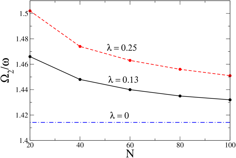
Figure 1: Quadrupole frequency $\Omega_{2}$ of the unitary Fermi gas with $N$ atoms under harmonic confinement of frequency $\omega$. Three different values of the gradient coefficient ${\lambda}$. For $\lambda=0$ (TF limit): $\Omega_{2}=\sqrt{2}\omega$. Figure adapted from Ref. [20].

The results are shown in Fig. 1 where we plot the quadrupole frequency $\Omega_{2}$ as a function of the number $N$ of atoms for three values of the gradient coefficient $\lambda$. The trend shown in the figure is captured by the formula

$$\Omega_{2}=\omega\ \sqrt{2+6\,\alpha\,{\lambda\over N^{2/3}}\over 1+{3\over 2}\alpha\,{\lambda\over N^{2/3}}}\;,$$ (27)

where $\alpha=3(6/5)^{3/2}(3\pi^{2})^{2/3}\xi/5$. This expression is easily derived by using a time-dependent Gaussian variational approach [31] in the ETF action functional (22). In the limit $N\to\infty$ it gives the TF result $\Omega=\sqrt{2}\omega$ [2], while in the limit $N\to 0$ it gives $\Omega=2\omega$, which is the quadrupole oscillation frequency of non-interacting atoms [2].

5 Shock waves

One of the basic problems in physics is how density perturbations propagate through a material. In addition to the well-known sound waves, there are shock waves characterized by an abrupt change in the density of the medium: they produce, after a transient time, an extremely large density gradient (the shock). Shock waves are ubiquitous and have been studied in many different physical systems [32; 33]. Here we investigate the formation and dynamics of shock waves in the unitary Fermi gas by using the zero-temperature equations of generalized superfluid hydrodynamics, inspired by the very recent observation of nonlinear hydrodynamic waves in the collision between two strongly interacting Fermi gas clouds of ⁶Li atoms [34].

Let us consider the unitary Fermi gas with constant density $\bar{n}$ with $U({\bf r})=0$. Experimentally this configuration can be obtained with a very large square-well potential (or a similar external trapping), such that in the model one can effectively impose periodic boundary conditions instead of the vanishing ones. A density variation along the $z$ axis with respect to the uniform configuration $\bar{n}$ can be experimentally created by using a blue-detuned (bright perturbation) or a red-detuned (dark perturbation) laser beam [1; 2]. In practice, we perform the following factorization

$$n({\bf r},t)=n_{\bot}(x,y)\,n_{\parallel}(z,t)\;,$$ (28)

by imposing also

$$n_{\bot}(x,y)=\bar{n}_{\bot}$$ (29)

$$n_{\parallel}(z,t)=\bar{n}_{\parallel}\;\rho(z,t)$$ (30)

such that

$$n({\bf r},t)=\bar{n}\,\rho(z,t)$$ (31)

where $\bar{n}=\bar{n}_{\bot}\bar{n}_{\parallel}$, and $\rho(z,t)$ is the relative density, i.e. the localized axial modification with respect to the uniform density $\bar{n}$. We impose periodic boundary conditions along the $z$ axis, namely $\rho(z=L_{z},t)=\rho(z=-L_{z},t)$, with $2L_{z}$ the axial-domain length. We set ${\bf v}({\bf r},t)=(0,0,v(z,t))$ with $v(z,t)$ the velocity field such that $v(z=L_{z},t)=v(z=-L_{z},t)$. Moreover we impose that the initial localized wave packet satisfies the boundary conditions $\rho(z=\pm L_{z},t=0)=1$ and $v(z=\pm L_{z},t=0)=0$. Because the dimensional reduction is done assuming the uniformess in $x$,$y$ directions, we shall consider the propagation of a plane wave along the $z$ axis.

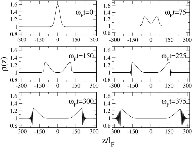
Figure 2: Time evolution of supersonic shock waves. Initial condition with $\sigma/l_{F}=18$ and $\eta=0.3$. The curves give the relative density profile $\rho(z)$ at subsequent frames, where $l_{F}=\sqrt{\hbar^{2}/(m\epsilon_{F})}$ is the Fermi length and $\omega_{F}=\epsilon_{F}/\hbar$ is the Fermi frequency. Figure adapted from Ref. [22].

Inserting Eq. (31) into Eqs. (20) and (21) one finds the 1D hydrodynamic equations for the axial dynamics of the superfluid, given by

$${\dot{\rho}}+v\rho^{\prime}+v^{\prime}\rho=0\;,$$ (32)

$${\dot{v}}+vv^{\prime}+{c_{ls}(\rho)^{2}\over\rho}\rho^{\prime}=0\;,$$ (33)

where dots denote time derivatives, primes space derivatives, and

$$c_{ls}(\rho)=c_{s}\rho^{1/3}$$ (34)

is the local sound velocity, with $c_{s}=c_{ls}(1)=\sqrt{\xi/3}v_{F}$ the bulk sound velocity, $v_{F}=\sqrt{2\epsilon_{F}/m}$ is bulk Fermi velocity and $\epsilon_{F}={\hbar^{2}\over 2m}(3\pi^{2}\bar{n})^{2/3}$ the bulk Fermi energy.

We solve Eqs. (32) and (33) by using a Crank-Nicolson finite-difference predictor-corrector algorithm [35] with the initial condition given by

$$\rho(z,t=0)=1+2\eta\ e^{-z^{2}/(2\sigma^{2})}\;,$$ (35)

and $v(z,t=0)=0$, where $\bar{n}$ is the bulk density. In Fig. 2 we plot the time evolution obtained with $\sigma/l_{F}=18$ and $\eta=0.3$, with $\sqrt{\hbar^{2}/(m\epsilon_{F})}$ the Fermi length of the bulk system. The figure displays the density profile $\rho(z)$ at subsequent times. Note the splitting on the initial bright wave packet into two bright travelling waves moving in opposite directions. There is a deformation of the two waves with the formation of a quasi-horizontal shock-wave front. Eventually, this front spreads into wave ripples. We have carefully checked that these ripples are not an artefact of the numerical scheme. Notice that before the shock both amplitude and velocity of the two maxima of the two waves are practically constant during time evolution. In particular, as we have recently shown [22] that the amplitude of the extrema can be written $A(\eta)=1+\eta$ while the velocity of the extrema reads

$$V(\eta)=\pm c_{s}\left(4(1+\eta)^{1/3}-3\right)\;.$$ (36)

Taking $\eta=0$ the velocity of the impulse extrema reduces to the sound velocity: $V(0)=c_{s}=\sqrt{\xi/3}v_{F}$. Moreover, bright perturbations ($\eta>0$) move faster than dark ones ($\eta<0$), and the Mach number $M=V(\eta)/V(0)$ of these perturbations in the unitary Fermi gas is simply

$$M=4(1+\eta)^{1/3}-3\;.$$ (37)

For $M>1$, which means $\eta>0$ (bright perturbation), one has supersonic waves, while for $0\leq M<1$, which means $\eta<0$ (dark perturbation), one has subsonic waves. In the upper panel of Fig. 3 we plot the Mach number $M$ as function of the amplitude $\eta$ of the perturbation. Note that since $2\eta$ is the amplitude of the initial condition, see Eq. (35), the region $\eta\leq-1/2$ is unphysical.

Let us consider a bright perturbation ($\eta>0$) moving to the right. The speed of impulse maximum $V(\eta)$ is bigger than the speed of its tails $V(0)$. As a result the impulse self-steepens in the direction of propagation and a shock wave front takes place. The breaking-time $T_{s}$ required for such a process can be estimated as follows: the shock wave front appears when the distance difference traveled by lower and upper impulse parts is equal to the impulse half-width $\sigma/2$. This criterion gives [22]

$$T_{s}={\sigma\over 2c_{s}((1+\eta)^{1/3}-1)}\;.$$ (38)

In the lower panel of Fig. 3 we plot the period $T_{s}$ as a function of the amplitude $\eta$ of the perturbation. The figure shows that as $\eta$ goes to zero the period $T_{s}$ goes to infinity; in fact, in this limit the shock wave reduces to a sonic wave (sound wave) which does not produce a shock.

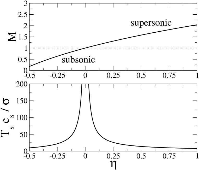
Figure 3: Upper panel: Mach number $M=v_{max}/c_{s}$ as a function of the amplitude $\eta$ of the perturbation (solid line). Lower panel: period $T_{s}$ of formation (breaking time) of the shock-wave front as a function of the amplitude $\eta$ of the perturbation. $T_{s}$ is in units of $\sigma/c_{s}$, where $\sigma$ is the width of the perturbation and $c_{s}=\sqrt{\xi/3}v_{F}$ is the bulk speed of sound, with $v_{F}$ the Fermi velocity. Figure adapted from Ref. [22].

6 Conclusions

We have shown that the ETF functional of the unitary Fermi gas can be used to determine ground-state properties of the system in a generic external potential $U({\bf r})$. Moreover, the time-dependent version of this EFT function, that is the generalized hydrodynamics equations, can be applied to calculate sound waves, collective modes and also shock waves. Our generalized superfluid hydrodynamics is reliable when the effects of the temperature $T$ are negligible, namely if $T\ll T_{c}$, with $T_{c}$ the critical temperature of the superfluid-normal phase transition ($T_{c}\simeq 0.2\ T_{F}$, and $T_{F}\simeq 10^{-7}$ Kelvin for dilute alkali-metal atoms). As previously discussed, recently an observation of nonlinear hydrodynamic waves has been reported in collisions between two strongly interacting Fermi gas clouds of ⁶Li atoms [34]. The experiment shows the formation of density gradients, which are nicely reproduced by hydrodynamic equations with a phenomenological viscous term [34]. Nevertheless, the role of dissipation is questionable in this case since the ultracold unitary Fermi gas is known to be an example of an almost perfect fluid [36]. We plan to simulate the collision between two strongly interacting Fermi-gas clouds of ⁶Li atoms by using our single-orbital time-dependent density functional. In particular, we aim to demonstrate that it is possible to reproduce the recent experimental results without the inclusion of a phenomenological dissipative term. Another interesting related problem is the determination of the surface tension of the unitary Fermi superfluid. We shall consider a semi-infinite domain, derive the density profile of the system by using our density functional, and obtain the surface tension as the grand potential energy difference between the actual configuration and the uniform asymptotic one. Finally, we shall compare our result with previous determinations based on microscopic calculations of the normal-superfluid interface in population-imbalanced Fermi gases [37].

- [1] A.J. Leggett, Quantum liquids (Cambridge Univ. Press, Cambridge, 2006).
- [2] S. Giorgini, L. P. Pitaevskii, and S. Stringari, Rev. Mod. Phys. 80, 1215 (2008).
- [3] A. Bulgac, M. Mc Neil Forbes, and P. Magierski, in BCS-BEC Crossover and the Unitary Fermi Gas, Lecture Notes in Physics, vol. 836, Ed. by W. Zwerger (Springer, Berlin, 2011).
- [4] A. Bulgac and Y. Yu, Phys. Rev. Lett. 91, 190404 (2003).
- [5] A. Bulgac, Phys. Rev. A 76, 040502(R) (2007).
- [6] T. Papenbrock, Phys. Rev. A 72, 041603(R) (2005); A. Bhattacharyya and T. Papenbrock, Phys. Rev. A 74, 041602(R) (2006).
- [7] L. Salasnich and F. Toigo, Phys. Rev. A 78, 053626 (2008); L. Salasnich and F. Toigo, Phys. Rev. A 82, 059902(E) (2010).
- [8] S.K. Adhikari and L. Salasnich, Phys. Rev. A 78 043616 (2008); L. Salasnich, Laser Phys. 19, 642 (2009); S.K. Adhikari and L. Salasnich, New J. Phys. 11, 023011 (2009).
- [9] C.F. von Weizsäcker, Zeit. Phys. 96, 431 (1935).
- [10] N.H. March and M. P. Tosi, Proc. R. Soc. A 330, 373 (1972).
- [11] E. Zaremba and H.C. Tso, Phys. Rrev. B 49, 8147 (1994).
- [12] Y.E. Kim and A.L. Zubarev, Phys. Rev. A 70, 033612 (2004); N. Manini and L. Salasnich, Phys. Rev. A 71, 033625 (2005); G. Diana, N. Manini, and L. Salasnich, Phys. Rev. A 73, 065601 (2006).
- [13] M.A. Escobedo, M. Mannarelli and C. Manuel, Phys. Rev. A 79, 063623 (2009).
- [14] E. Lundh and A. Cetoli, Phys. Rev. A 80, 023610 (2009).
- [15] G. Rupak and T. Schäfer, Nucl. Phys. A 816, 52 (2009).
- [16] S.K. Adhikari, Laser Phys. Lett. 6, 901 (2009).
- [17] W.Y. Zhang, L. Zhou, and Y.L. Ma, EPL 88, 40001 (2009).
- [18] A. Csordas, O. Almasy, and P. Szepfalusy, Phys. Rev. A 82, 063609 (2010).
- [19] S. N. Klimin, J. Tempere, and J.P.A. Devreese, J. Low Temp. Phys. 165, 261 (2011).
- [20] L. Salasnich, F. Ancilotto, and F. Toigo, Laser Phys. Lett. 7, 78 (2010).
- [21] F. Ancilotto, L. Salasnich, and F. Toigo, Phys. Rev. A 79, 033627 (2009).
- [22] L. Salasnich, EPL 96, 40007 (2011).
- [23] L. Salasnich, Phys. Rev. A 82, 063619 (2010).
- [24] L. Salasnich and F. Toigo, J. Low Temp. Phys. 165, 239 (2011).
- [25] K.M. O’Hara et al., Science 298, 2179 (2002).
- [26] M.W. Zwierlein et al., Science 311, 492 (2006); M.W. Zwierlein et al., Nature 442, 54 (2006).
- [27] S.-Y. Chang and G.F. Bertsch, Phys. Rev. A 76, 021603(R) (2007).
- [28] D. Blume, J. von Stecher, and C. H. Greene, Phys. Rev. Lett. 99, 233201 (2007); J. von Stecher, C.H. Greene, and D. Blume, Phys. Rev. A 76, 053613 (2007).
- [29] A. Bulgac, J.E. Drut, and P. Magierski, Phys. Rev. Lett 96, 090404 (2006); ibid 99, 120401 (2007); Phys. Rev. A 78, 023625 (2008).
- [30] Y. Castin, Comptes Rendus Physique 5, 407 (2004).
- [31] L. Salasnich, Int. J. Mod. Phys. B 14, 1 (2000).
- [32] L.D. Landau and E.M. Lifshitz, Fluid Mechanics (Pergamon Press, London, 1987).
- [33] G.G. Whitham, Linear and Nonlinear Waves (Wiley, New York, 1974).
- [34] J. Joseph, J. Thomas, M. Kulkarni, and A. Abanov, Phys. Rev. Lett. 106, 150401 (2011).
- [35] E. Cerboneschi, R. Mannella, E. Arimondo, and L. Salasnich, Phys. Lett. A 249, 495 (1998); G. Mazzarella and L. Salasnich, Phys. Lett. A 373 4434 (2009).
- [36] C. Cao, E Elliott, H Wu, and J E Thomas, New J. Phys. 13, 075007 (2011).
- [37] H. Caldas, J. Stat. Mech. P11012 (2007); A. Kryjevski, Phys. Rev. A 78, 043610 (2008); S.K. Baur, Sourish Basu, T.N. De Silva and E.J. Mueller, Phys. Rev. A 79, 063628 (2009).