A Faster Pseudo-Primality Test

Abstract.

We propose a pseudo-primality test using cyclic extensions of ${\mathbb{Z}}/n{\mathbb{Z}}$. For every positive integer $k\leqslant\log n$, this test achieves the security of $k$ Miller-Rabin tests at the cost of $k^{1/2+o(1)}$ Miller-Rabin tests.

1. Introduction

Pseudo-primality tests

The most commonly used algorithm for prime detection is the so called Miller-Rabin test. It is a Monte Carlo probabilistic test of compositeness, also called a pseudo-primality test (see Papadimitrou’s book [14, page 254] for the definition of a Monte Carlo algorithm). A pseudo-primality test is a process based on a mathematical statement, the compositeness criterion, which gives a forecast (prime or composite) about a given integer $n$. From the compositeness criterion, one constructs for every odd integer $n$, a finite set $W_{n}$ of witnesses, and a map

$$\mathrm{P}_{n}:W_{n}\rightarrow\{{\mathrm{composite}},{\mathrm{prime}}\}$$

which provides information about the compositeness of $n$ from witnesses $x$ in $W_{n}$. When $n$ is prime ${\mathrm{P}}_{n}(x)={\mathrm{prime}}$ for every witness $x$ in $W_{n}$. So there are only good witnesses in that case. If $n$ is composite, $x$ is a witness in $W_{n}$, and ${\mathrm{P}}_{n}(x)={\mathrm{prime}}$ we say that $x$ is a bad witness. The test picks a random witness $x$ in $W_{n}$ and evaluates ${\mathrm{P}}_{n}(x)$. Two important characteristics of a pseudo-primality test are the run-time complexity $n\mapsto T(n)$ of the algorithm evaluating $\mathrm{P}_{n}$, and the density $n\mapsto\mu(n)$ of bad witnesses.

To be quite rigorous, we do not need to be able to evaluate $\mathrm{P}_{n}$ in deterministic time $T(n)$. We are content with a Las Vegas probabilistic algorithm that on input $n$, runs in time $T(n)$, and returns with probability $\geqslant 1/2$ at least one of the following two things

• a proof that $n$ is composite,

• the value of $\mathrm{P}_{n}$ at a random (with uniform probability) element in $W_{n}$.

If this is the case, we say that the test $\mathrm{P}$ has complexity $n\mapsto T(n)$ and density $n\mapsto\mu(n)$. See [14, page 256] for the definition of a Las Vegas algorithm.

The Miller-Rabin test

We assume $n$ is odd. The set $W_{n}$ of witnesses for the Miller-Rabin test is $({\mathbb{Z}}/n{\mathbb{Z}})^{*}$. The associated map

$${\mathrm{MR}}_{n}:({\mathbb{Z}}/n{\mathbb{Z}})^{*}\rightarrow\{{\mathrm{composite}},{\mathrm{prime}}\}$$

is defined by ${\mathrm{MR}}_{n}(x)={\mathrm{prime}}$ if and only if $x^{m}=1$ or $x^{m2^{i}}=-1$ for some $0\leqslant i<k$. Here $m$ is the largest odd divisor of $n-1$ and $n-1=m2^{k}$. We call ${\mathrm{MR}}_{n}$ a Miller-Rabin map. It is clear that if $n$ is prime then ${\mathrm{MR}}(x)={\mathrm{prime}}$ for every $x$ in $W_{n}$. In case $n$ is composite, the density $\mu_{{\mathrm{MR}}}(n)$ of bad witnesses is bounded from above by $1/4$ (see [15, Theorem $2.1$]). It will be important for us that this density is actually bounded from above by $2^{1-t}$ (see [15, proof of Theorem $2.1$]) where $t$ is the number of prime divisors of $n$. The complexity $T_{{\mathrm{MR}}}(n)$ is bounded from above by $(\log n)^{2+o(1)}$ using fast exponentiation and fast arithmetic. If we run $k$ independent Miller-Rabin tests, the probability of missing a composite number is $\leqslant 4^{-k}$ and the complexity is $k(\log n)^{2+o(1)}$.

A faster pseudo-primality test

In this article we prove the following theorem.

Theorem 1 (A faster test).

There exist a function $\varepsilon:{\mathbb{R}}\rightarrow{\mathbb{R}}$ in the class $o(1)$ and a probabilistic algorithm (described in Section 5.1) that takes as input an odd integer $n$ and an integer $\lambda$ such that $1\leqslant\lambda\leqslant{\log n}$, runs in time

$$T=(\log n)^{2+\varepsilon(n)}\lambda^{\frac{1}{2}+\varepsilon(\lambda)},$$

an returns ${\mathrm{prime}}$ always if $n$ is prime, and with probability

$$\leqslant 2^{-\lambda}$$

if $n$ is composite.

This algorithm achieves the security of $\lambda/2$ Miller-Rabin tests at the cost of $\lambda^{1/2+o(1)}$ such tests. The two main ingredients of our test are the product of pseudo-primality tests and a primality criterion involving an extension of the ring ${\mathbb{Z}}/n{\mathbb{Z}}$.

Products

We introduce the associative composition law

$$\vee:\{{\mathrm{composite}},{\mathrm{prime}}\}\times\{{\mathrm{composite}},{\mathrm{prime}}\}\rightarrow\{{\mathrm{composite}},{\mathrm{prime}}\}$$

with table

$\vee$	composite	prime
composite	composite	composite
prime	composite	prime

Let $r\geqslant 2$ be an integer and let $\mathrm{P}_{n}^{i}:W_{n}^{i}\rightarrow\{{\mathrm{composite}},{\mathrm{prime}}\}$ be $r$ pseudo-primality tests. One defines the product test

$${\mathrm{P}}_{n}=\vee_{1\leqslant i\leqslant r}{\mathrm{P}}_{n}^{i}$$

as

A witness for ${\mathrm{P}}$ is an $r$-uple of witnesses, one for each of the $r$ tests ${\mathrm{P}}_{n}^{1}$, …, ${\mathrm{P}}_{n}^{r}$. For $n$ composite, a witness is bad if and only if all its $r$ coordinates are bad witnesses. So the density of bad witnesses is the product of all the densities for every tests. And the complexity is bounded by the sum of all $r$ complexities, times $\lceil\log_{2}r\rceil+1$. This last factor is natural when chaining Las Vegas algorithms. In order to make sure that the resulting algorithm still succeeds with probability $\geqslant 1/2$ we must repeat a little bit every step. As a special case, we consider the $r$-th power $\vee^{r}{\mathrm{P}}$ of a single test ${\mathrm{P}}$ with complexity $T$ and density $\mu$. The density of bad witnesses for $\vee^{r}{\mathrm{P}}$ is equal to $\mu^{r}$, and its complexity is $r\times T\times(\lceil\log_{2}r\rceil+1)$.

A compositeness criterion

The test in Theorem 1 is based on the following compositeness criterion.

Theorem 2 (Compositeness criterion).

Let $n\geqslant 2$ be an integer. Let $S\supset{\mathbb{Z}}/n{\mathbb{Z}}$ be a faithful, finite, associative, commutative ${\mathbb{Z}}/n{\mathbb{Z}}$-algebra with unit. Let $\sigma$ be an ${\mathbb{Z}}/n{\mathbb{Z}}$-endomorphism of $S$. Let $\Omega\subset S$ be a subset of $S$ such that the smallest ${\mathbb{Z}}/n{\mathbb{Z}}$-subalgebra of $S$ containing $\Omega$ and stable under the action of $\sigma$ is $S$ itself. Assume $\omega^{n}=\sigma(\omega)$ for every $\omega$ in $\Omega$. If $n$ is prime, then for every $x$ in $S$ we have $x^{n}=\sigma(x)$.

• Let $T$ be the subset of $S$ consisting of all $x$ such that $x^{n}=\sigma(x)$. Clearly $T$ contains $\Omega$. If $n$ is prime, then $T$ contains ${\mathbb{Z}}/n{\mathbb{Z}}$ and is stable under addition, multiplication, and action of $\sigma$. So $T=S$ and we have $x^{n}=\sigma(x)$ for every $x$ in $S$.

$\square$

Theorem 2 provides a compositeness criterion since the existence of an $x$ in $S$ such that $x^{n}\not=\sigma(x)$ implies that $n$ is not a prime. We call the associated pseudo-primality test a Galois test. The set $W_{n}$ of witnesses is the group $S^{*}$ of units in $S$. The map ${\mathrm{P}}_{n}$ is defined by ${\mathrm{P}}_{n}(x)={\mathrm{prime}}$ if $\sigma(x)=x^{n}$ and ${\mathrm{P}}_{n}(x)={\mathrm{composite}}$ otherwise. In that situation, we call ${\mathrm{P}}_{n}$ a Galois map. In case $n$ is composite, those $x$ in $S$ for which

$$x^{n}=\sigma(x)$$ (1)

are the bad witnesses.

Plan

We will show in Section 2 that one can bound from above the density of bad witnesses among the units of the algebra $S$ in Theorem 2, at least when $S$ is a cyclic extension of ${\mathbb{Z}}/n{\mathbb{Z}}$. We will use the Galois module structure of the unit group of such an extension. The resulting pseudo-primality test is presented an analyzed in Section 3. Section 4 explains how to efficiently construct the cyclic ${\mathbb{Z}}/n{\mathbb{Z}}$-algebras required by our test. Theorem 1 is proven in Section 5.1. Implementation details are given in Section 5.2. We present the results of our experiments in Section 6.

Context

There exist many (families of) algorithms for prime detection. A recent survey can be found in Schoof’s article [15]. The first polynomial time deterministic algorithm for distinguishing prime numbers from composite numbers is due to Agrawal, Kayal and Saxena [2]. An improvement of this algorithm, due to Lenstra and Pomerance [12], has deterministic complexity $(\log n)^{6+o(1)}$. This is the best known unconditional result for deterministic algorithms. There exists a deterministic algorithm with complexity $(\log n)^{4+o(1)}$ under the generalized Riemann hypothesis, as observed by Miller in [13]. Dan Bernstein has found [5] a Las Vegas probabilistic algorithm with complexity $(\log n)^{4+o(1)}$. See also Avanzi and Mihăilescu [4]. The correctness and running time of this algorithm does not depend on the truth of any unproved conjecture. It is unconditional.

Notation

In this paper, the notation $\Theta$ stands for a positive absolute constant. Any statement containing this symbol becomes true if the symbol is replaced in every occurrence by some large enough real number. Similarly, the notation $\varepsilon(x)$ stands for a real function of the real parameter $x$ alone, belonging to the class $o(1)$.

2. Cyclic extensions of ${\mathbb{Z}}/n{\mathbb{Z}}$

Let $n\geqslant 3$ be an odd integer and set $R={\mathbb{Z}}/n{\mathbb{Z}}$. A cyclic extension of $R$ is a Galois extension $S$ of $R$ in the sense of [8, Chapter III], with finite cyclic Galois group ${\mathcal{G}}$. We denote by $d$ the order of ${\mathcal{G}}$, and let $\sigma$ be a generator of it. The Galois property implies [8, Chapter III, Corollary 1.3] that $S$ is a projective $R$-module of constant rank $d$. Since $R$ is semi-local we deduce [6, II.5.3, Proposition 5] that $S$ is free of rank $d$. The sub-algebra $S^{\mathcal{G}}$ consisting of elements in $S$ fixed by $\sigma$ is $R$ itself [8, Chapter III, Proposition 1.2]. And $S$ is a separable $R$-algebra in the sense that it is projective as a module over $S\otimes_{R}S$. We deduce [3, Theorem 2.5.] that $S$ is an unramified extension of $R$. And $S$ is a free $R[{\mathcal{G}}]$-module of rank $1$. Equivalently there exists a normal basis [7, Theorem 4.2.]. In this section we study the group of units of such an algebra and count the solutions to Equation (1) in it. In Paragraph 2.1 we localize at a prime $p$ and we study the Frobenius action on the residue algebra. We decompose the unit group as a direct product. The $p$-part is studied in Paragraph 2.2, and the prime to $p$-part is studied in Paragraph 2.3. In Paragraph 2.4 we deduce an estimate for the number of bad witnesses. We refer to the book by DeMeyer and Ingraham [8] for general properties of Galois extensions, and to Lenstra [10, 11] for their use in the context of primality testing.

2.1. The structure of $S^{*}$ as a ${\mathbb{Z}}[{\mathcal{G}}]$-module

We write $n=\prod_{p}p^{v_{p}}$ the prime decomposition of $n$. If $p$ and $q$ are two distinct primes dividing $n$, then $p^{v_{p}}S+q^{v_{q}}S=S$. Furthermore, the intersection of all $p^{v_{p}}S$ for $p$ dividing $n$ is zero. So $S$ is isomorphic to the product

$$\prod_{p|n}S/p^{v_{p}}S=\prod_{p|n}S_{p},$$

and this decomposition is an isomorphism of ${\mathbb{Z}}[{\mathcal{G}}]$-modules. So we can and will assume now that $n=p^{v}$ is a prime power.

We set ${\bf L}=S/pS$ and ${\bf K}=R/pR={\mathbb{Z}}/p{\mathbb{Z}}$. Since $pS\cap R=pR$, the ring ${\bf L}$ is a faithful ${\bf K}$-algebra. The $R$-automorphism $\sigma:S\rightarrow S$ induces a ${\bf K}$-automorphism of ${\bf L}$ that we call $\sigma$ also. The ${\bf K}$-algebra ${\bf L}$ has dimension $d$ and is Galois with group ${\mathcal{G}}$ [11, Proposition 2.7.]. From ${\bf K}={\bf L}^{\mathcal{G}}$ we deduce [6, Chapitre 5, paragraphe 1, numéro 9, proposition 22] that ${\bf L}$ is integral over ${\bf K}$. Let ${\mathfrak{p}}$ be a prime ideal in ${\bf L}$. The intersection ${\mathfrak{p}}\cap{\bf K}$ is a prime ideal in ${\bf K}$, so it is equal to $0$. Since $0$ is maximal in ${\bf K}$, the ideal ${\mathfrak{p}}$ is maximal in ${\bf L}$ [6, Chapitre 5, paragraphe 2, numéro 1, Proposition 1]. Thus ${\bf L}$ is a ring of dimension $0$. Since ${\bf L}$ is noetherian, it is an artinian ring [6, Chapitre 4, paragraphe 2, numéro 5, Proposition 9]. The automorphism $\sigma$ acts transitively on the set of prime ideals in ${\bf L}$ [6, Chapitre 5, paragraphe 2, numéro 2, Théorème 2]. We denote by ${\mathcal{G}}^{Z}$ (resp. ${\mathcal{G}}^{T}$) the decomposition group (resp. inertia group) of all these prime ideals. The Galois property [8, Proposition 1.2] implies that the inertia group is trivial. Let $f$ be the order of ${\mathcal{G}}^{Z}$. We check that $d=fm$ where $m$ is the number of prime ideals in ${\bf L}$. Let ${\mathfrak{p}}_{0}$, ${\mathfrak{p}}_{1}$, …, ${\mathfrak{p}}_{m-1}$ be all these prime ideals. They are pairwise comaximal: for $i\not=j$ we have ${\mathfrak{p}}_{i}+{\mathfrak{p}}_{j}={\bf L}$. The radical of ${\bf L}$ is

$${\mathfrak{N}}=\bigcap_{0\leqslant i\leqslant m-1}{\mathfrak{p}}_{i}=\prod_{0\leqslant i\leqslant m-1}{\mathfrak{p}}_{i}=0,$$

because ${\bf L}$ is unramified over ${\bf K}$. So the map

$${\bf L}\longrightarrow\prod_{0\leqslant i\leqslant m-1}{\bf L}/{\mathfrak{p}}_{i}$$

is an isomorphism of ${\mathbb{Z}}[{\mathcal{G}}^{Z}]$-modules. For every $i$ in $\{0,1,\ldots,m-1\}$, the decomposition group ${\mathcal{G}}^{Z}$ is isomorphic to the group of ${\bf K}$-automorphisms of the residue field ${\bf M}_{i}={\bf L}/{\mathfrak{p}}_{i}$ [6, Chapitre 5, paragraphe 2, numéro 2, Théorème 2]. The Frobenius automorphism $\Phi_{i}$ of ${\bf M}_{i}={\bf L}/{\mathfrak{p}}_{i}$ is the reduction modulo ${\mathfrak{p}}_{i}$ of some power $\sigma^{z_{i}m}$ of $\sigma$ generating ${\mathcal{G}}^{Z}$. Especially, for every $a$ in ${\bf L}$, one has $\sigma^{z_{0}m}(a)=a^{p}\bmod{\mathfrak{p}}_{0}$ for some integer $z_{0}$. We let $\sigma$ act on the above congruence and deduce that $z_{0}=z_{1}=\cdots=z_{d-1}\bmod f$ because $\sigma$ acts transitively on the set of primes. So there exists a prime to $f$ integer $z$ such that for every element $x$ in ${\bf L}$ we have

$$x^{p}=\sigma^{zm}(x)\,.$$

We set

$${\mathbb{U}}=\{x\in S|x\equiv 1\bmod p\}.$$

This is a subgroup of the group $S^{*}$ of units in $S$, and even a ${\mathbb{Z}}[{\mathcal{G}}]$-module. We have an exact sequence of ${\mathbb{Z}}[{\mathcal{G}}]$-modules

$$1\rightarrow{\mathbb{U}}\rightarrow S^{*}\rightarrow(S/pS)^{*}\rightarrow 1.$$

While the group ${\mathbb{U}}$ is a $p$-group, the group $(S/pS)^{*}={\bf L}^{*}$ has order prime to $p$. So ${\mathbb{U}}$ is the $p$-Sylow subgroup of $S^{*}$. We denote by ${\mathbb{V}}$ the product of all $q$-Sylow subgroups of $S^{*}$ for $q\not=p$. Then

$$S^{*}={\mathbb{U}}\times{\mathbb{V}}$$ (2)

and this decomposition is an isomorphism of ${\mathbb{Z}}[{\mathcal{G}}]$-modules because both ${\mathbb{U}}$ and ${\mathbb{V}}$ are characteristic subgroups of $S^{*}$. Furthermore, ${\mathbb{V}}$ is isomorphic to $(S/pS)^{*}$ as a ${\mathbb{Z}}[{\mathcal{G}}]$-module. We study either factors separately.

2.2. The structure of ${\mathbb{U}}$

The two maps

and

are well defined. They are indeed polynomial maps (recall that $p$ is odd). In particular, both maps are equivariant for the action of ${\mathcal{G}}$. So $\mathop{\rm{Log}}\nolimits$ is an isomorphism between the ${\mathbb{Z}}[{\mathcal{G}}]$-modules $({\mathbb{U}},\times)$ and $(pS,+)$. And $\mathop{\rm{Exp}}\nolimits$ is the reciprocal map.

2.3. The structure of ${\mathbb{V}}$

Let ${\mathfrak{p}}$ be a prime in $S$ above $p$. We set ${\bf M}=S/{\mathfrak{p}}$. Recall that

$$pS=\prod_{0\leqslant k\leqslant m-1}\sigma^{k}({\mathfrak{p}}),$$

and there exists a prime to $f$ integer $z$ such that for every element $x$ in $S$ we have

$$x^{p}=\sigma^{zm}(x)\,\bmod p.$$

Let $1\leqslant t\leqslant f-1$ be the inverse of $z$ modulo $f$. Note that if $f=1$, we have $z=t=0$. We turn ${\bf M}^{m}$ into a ${\mathbb{Z}}[{\mathcal{G}}]$-module by setting

$$\sigma.(x_{0},x_{1},\ldots,x_{m-1})=(x_{1},x_{2},\ldots,x_{m-1},x_{0}^{p^{t}}).$$ (3)

The map

is an isomorphism of ${\mathbb{Z}}[{\mathcal{G}}]$-module between $S/pS$ and ${\bf M}^{m}$. So ${\mathbb{V}}$ and $({\bf M}^{*})^{m}$ are isomorphic as ${\mathbb{Z}}[{\mathcal{G}}]$-modules.

2.4. Counting bad witnesses

We now show that in many cases one can bound from above the density of bad witnesses among the units of $S$.

Theorem 3 (Density of bad witnesses).

Let $A>2$ and $B\geqslant 3$ be two real numbers. Let $n\geqslant 3$ be an integer. Assume that every prime dividing $n$ is bigger than or equal to $B$. Assume that $n$ is not a prime power. Let $S\supset{\mathbb{Z}}/n{\mathbb{Z}}$ be a cyclic $({\mathbb{Z}}/n{\mathbb{Z}})$-algebra of dimension $d$. Let $\sigma$ be a generator of the Galois group ${\mathcal{G}}$. Assume that $n$ has a prime power divisor $p^{v}$ satisfying

$$v\log p\geqslant\frac{A\log n}{d}.$$ (4)

Then the density

$$\mu_{S}=\frac{\#\{x\in S^{*}|\sigma(x)=x^{n}\}}{\#S^{*}}$$

of bad witnesses among the units of $S$ is such that

$$\mu_{S}\leqslant{p^{-\frac{vd}{2}(1-\frac{2}{A}-\frac{4}{B})}}\leqslant n^{-\frac{A}{2}(1-\frac{2}{A}-\frac{4}{B})}.$$ (5)

• We count the solutions to Equation (1) in $S^{*}$. Since $S$ is isomorphic to the product of all $S_{p}$ for $p$ a prime dividing $n$, we fix such a prime $p$ and count the solutions to Equation (1) in $S_{p}^{*}$. Using the decomposition in Equation (2) we then reduce to counting solutions in the subgroups ${\mathbb{U}}$ and ${\mathbb{V}}$.

If $x\in{\mathbb{U}}$ is a solution to Equation (1) then $x^{n^{d}}=x$. Since ${\mathbb{U}}$ is a $p$-group and $p$ divides $n$ we deduce that $x=1$.

According to Section 2.3, the $R[{\mathcal{G}}]$-module ${\mathbb{V}}$ is isomorphic to $[(S/{\mathfrak{p}}S)^{*}]^{m}$ where $m$ is the number of prime ideals in $S$ above $p$, and ${\mathfrak{p}}$ is one of them, and the action of ${\mathcal{G}}$ is given by Equation (3). It is clear that any solution $x$ to Equation (1) in the latter $R[{\mathcal{G}}]$-module is characterized by its first coordinate $x_{0}$ and this coordinate must be a $|n^{m}-p^{t}|$-th root of unity in the field $S/{\mathfrak{p}}S$. Since the latter field has cardinality $p^{f}$ we deduce that the number of solutions to Equation (1) in ${\mathbb{V}}$ is

$$\gcd(n^{m}-p^{t},p^{f}-1).$$

The density of bad witnesses is thus

$$\mu_{S}=\prod_{p|n}\frac{\gcd(n^{m}-p^{t},p^{f}-1)}{(p^{f}-1)^{m}p^{(v-1)d}},$$ (6)

where the integers $f,m,v$ and $t$ depend on $p$. This density is bounded from above by any term in the product (6). So let $p$ be a prime divisor of $n$ such that $v\log p\geqslant\frac{A\log n}{d}$. Let $m$ be the number of prime ideals in $S$ above $p$.

We first assume that $m\geqslant 2$, so $p$ splits in $S$. Then the density of bad witnesses is bounded from above by ${1}/{(p^{f}-1)^{m-1}p^{(v-1)d}}$. We check that

$$N-1\geqslant N^{(1-\frac{2}{B})},$$ (7)

for every integer $N\geqslant B$. So $p^{f}-1\geqslant p^{{f}(1-\frac{2}{B})}$. Since $m-1\geqslant m/2$, we find

$$\mu_{S}\leqslant{1}/{p^{\frac{d}{2}(1-\frac{2}{B})+(v-1)d}}.$$

The result follows.

We now assume that $m=1$, so $p$ is inert in $S$ and $f=d$. We first prove the following inequality

$$\gcd(n-p^{t},p^{d}-1)\leqslant{np^{\frac{d}{2}}}.$$ (8)

Indeed, if $1\leqslant t\leqslant\frac{d}{2}$, Inequality (8) is granted because $1\leqslant|n-p^{t}|\leqslant{\mathop{{\rm max}}\nolimits}(n,p^{t})\leqslant np^{t}$. In case $\frac{d}{2}<t\leqslant d-1$, we call $w$ the unique integer in $[1,d[$ that is congruent to $-t$ modulo $d$. We have

$$\gcd(n-p^{t},p^{d}-1)=\gcd(np^{w}-1,p^{d}-1).\\$$ (9)

Since $w\leqslant(d-1)/2$, the right hand side of (9) is bounded from above by $np^{\frac{d}{2}}$ as was to be shown. So Inequality (8) holds true in either case, and Inequality (5) follows using Equation (6), Equation (4), and Inequality (7).

$\square$

3. An efficient pseudo-primality test

A consequence of Theorem 3 is that a compositeness criterion as Theorem 2, when implemented with a cyclic $({\mathbb{Z}}/n{\mathbb{Z}})$-algebra of dimension $d$, is efficient, provided $n$ has a large prime power divisor $p^{v}$. On the other hand, we saw in Section 1 that the Miller-Rabin test is efficient when $n$ has many prime divisors. Combining these two tests we can construct a new probabilistic pseudo-primality test that takes advantage of either situation.

Fix two real numbers $A$ and $B$ such that $A>2$ and $B\geqslant 4A/(A-2)$. In particular $B>4$. Set $C=1-2/A-4/B$ and note that $C$ is positive.

Let $n$ be a positive integer. We assume $n$ is not a prime power, and every prime dividing $n$ is bigger than or equal to $B$. We choose two positive integers $r$ and $d$ and we construct a pseudo-primality test which is the product of $r$ Miller-Rabin tests and a Galois test of dimension $d$. We let $\delta=\log(d/A)/\log\log n$ so

$${d}=A(\log n)^{\delta}.$$

We let $\rho=\log(2A^{-1}r\log 2)/(\log\log n)$ so

$${r}=\frac{A(\log n)^{\rho}}{2\log 2}.$$

We assume

$$\left(1-\frac{A}{d}\right)(\log n)^{\delta+\rho}\leqslant C\log n,$$ (10)

or equivalently

$$dr\left(1-\frac{A}{d}\right)\leqslant\frac{A^{2}C\log n}{2\log 2}.$$

We call ${\mathrm{P}}_{1}:(({\mathbb{Z}}/n{\mathbb{Z}})^{*})^{r}\rightarrow\{{\mathrm{composite}},{\mathrm{prime}}\}$ the product of $r$ Miller-Rabin maps. And ${\mathrm{P}}_{2}:S^{*}\rightarrow\{{\mathrm{composite}},{\mathrm{prime}}\}$ a Galois map as in Theorem 2, associated with a cyclic algebra of dimension $d$. We set ${\mathrm{P}}={\mathrm{P}}_{1}\vee{\mathrm{P}}_{2}$. The density of bad witnesses for ${\mathrm{P}}$ is bounded from above by the densities of bad witnesses for ${\mathrm{P}}_{1}$ and ${\mathrm{P}}_{2}$. Let $p^{v}$ be the largest prime power dividing $n$. We set $\pi=\log(v\log p)/\log\log(n)$, so

$$\log p^{v}=(\log n)^{\pi}.$$

The number $t$ of prime divisors of $n$ satisfies

$$t>(\log n)/(v\log p)=(\log n)^{1-\pi}.$$

If

$$\delta+\pi\geqslant 1,$$

then $v\log p\geqslant\frac{A\log n}{d}$, and, according to Theorem 3, the density of bad witnesses for ${\mathrm{P}}_{2}$ is bounded from above by

$$p^{-\frac{vd}{2}(1-\frac{2}{A}-\frac{4}{B})}=\exp(-\frac{A}{2}(1-\frac{2}{A}-\frac{4}{B})(\log n)^{\delta+\pi}).$$ (11)

On the other hand, the density of bad witnesses for every Miller-Rabin test is $\leqslant{2^{-t+1}}$. The density of bad witnesses for $r$ such tests is at most

$$2^{-{r(t-1)}}\leqslant\exp(-\frac{A}{2}(1-\frac{1}{t})(\log n)^{1+\rho-\pi}).$$ (12)

Although we do not know the value of $\pi$, we can deduce from Equations (11) and (12) an upper bound for the density of bad witnesses of the product test ${\mathrm{P}}={\mathrm{P}}_{1}\vee{\mathrm{P}}_{2}$.

If $\pi$ lies in $[0,1-\delta[$ then Equation (11) gives nothing and Equation (12) gives an upper bound

$$\exp(-\frac{A}{2}(1-\frac{A}{d})(\log n)^{\rho+\delta}),$$

for the density of bad witnesses for ${\mathrm{P}}_{1}$.

If $\pi$ lies in $[1-\delta,1]$ then Equation (11) gives an upper bound

$$\exp(-\frac{A}{2}(1-\frac{2}{A}-\frac{4}{B})\log n),$$

for the density of bad witnesses for ${\mathrm{P}}_{2}$. Using Inequality (10) we find the upper bound

$$\exp(-\frac{A}{2}(1-\frac{A}{d})(\log n)^{\rho+\delta}),$$

in that case.

This discussion is illustrated in Figure 1 where the continuous line is the exponent of $\log n$ in Equation (12), the dashed line is the exponent of $\log n$ in Equation (11), and the bullet is the minimum of the maximum of the two functions.

Figure 1. The Miller-Rabin (continuous) and Galois (dashed) densities.

Theorem 4 (Density of the composed test).

Let $A$ and $B$ be two real numbers such that $A>2$ and $B\geqslant 4A/(A-2)$. Let

$$C=1-2/A-4/B.$$ (13)

Let $n$ be an integer that is not a prime power. Assume that $n$ has no prime divisor smaller than $B$. Let $r$ and $d$ be two positive integers such that

$$dr\left(1-\frac{A}{d}\right)\leqslant\frac{A^{2}C\log n}{2\log 2}$$ (14)

and let ${\mathrm{P}}$ be the composite test of $r$ Miller-Rabin tests and one Galois test of dimension $d$. The density of bad witnesses for ${\mathrm{P}}$ is bounded from above by

$$\leqslant 2^{-\frac{rd}{A}(1-\frac{A}{d})}.$$

Taking $A=2.1$, $B=1000$, and $d\geqslant 16$, we have $C\geqslant 0.043619$ and we obtain a density $\leqslant 2^{-0.41369rd}$ provided $rd\leqslant 0.13875\log n$.

Taking $A=4$, $B=1000$, and $d\geqslant 16$, we have $C\geqslant 0.496$ and we obtain a density $\leqslant 2^{-0.18rd}$ provided $rd\leqslant 5.72\log n$.

We note that the complexity of such a composed test is $(\log n)^{2+\varepsilon(n)}(r+d^{1+\varepsilon(d)})$ under the condition that arithmetic operations in the ${\mathbb{Z}}/n{\mathbb{Z}}$-algebra $S$ can be performed in quasi-linear time in the degree $d$. It is asymptotically optimal to take $d$ and $r$ as close as possible. We thus prove Theorem 1 provided we can efficiently construct a Galois extension of ${\mathbb{Z}}/n{\mathbb{Z}}$ with degree $d$ in some interval $[k,k^{1+\varepsilon(k)}]$. This is the purpose of the next Section 4.

Heuristics

There are many possible choices for the parameters $A$, $B$, $r$ and $d$ when using Theorem 4. We will explain in Section 5.2 how to choose them optimally. Here we just collect a few simple minded observations on what could be a reasonable choice. We take

$$B=8000.$$ (15)

Taking a too large $A$ is pointless. We recommend

$$2<A\leqslant 48.$$ (16)

In case we have a bigger value of $A$ it will be more efficient to take smaller values for $r$ and $d$ and repeat the whole test. We also suggest that

$$d\geqslant 2A,$$ (17)

otherwise we would better use $r$ Miller-Rabin tests only, and obtain better security at lower cost. It is reasonable also to have

$$d\leqslant r,$$ (18)

because the $r$ Miller-Rabin tests and the one Galois test have similar effect on the security. So the time devoted to the $r$ Miller-Rabin tests should not be smaller than the time devoted to the Galois test. Assume we want to bound from above the error probability by $2^{-\lambda}$ for some integer $\lambda$. We must have

$$\lambda\leqslant\frac{rd}{A}(1-\frac{A}{d}).$$ (19)

And we should have

$$\frac{rd}{A}(1-\frac{A}{d})\leqslant 2\lambda,$$ (20)

in order not to waste time.

We deduce from Equations (18), (20), (17), and (16) that

$$d\leqslant 2\sqrt{A\lambda}\leqslant 14\sqrt{\lambda}.$$ (21)

We deduce from Equations (19), (14), (13), and (16), that

$$\lambda\leqslant(0.9995A-2)\frac{\log_{2}n}{2}\leqslant 23\log_{2}n.$$ (22)

Under the reasonable hypotheses above, the smallest possible value for $A$ when applying Theorem 4 is thus

$$\left(2+\frac{2\lambda}{\log_{2}(n)}\right)/0.9995.$$

So we recommend to take

$$A=\left(2+\frac{2\lambda}{b-1}\right)/0.9995,$$ (23)

where

$$b=\lfloor\log_{2}(n)\rfloor+1,$$

is the number of bits of $n$.

4. Constructing algebras

In this section we prove the following theorem.

Theorem 5 (Constructing algebras).

There exist a function $\varepsilon:{\mathbb{R}}\rightarrow{\mathbb{R}}$ in the class $o(1)$ and a probabilistic (Las Vegas) algorithm that takes as input an odd integer $n$ and an integer $k$ such that $1\leqslant k\leqslant\log n$, runs in time $(\log n)^{2+\varepsilon(n)}$, and returns with probability $\geqslant 1/2$ at least one of the following two data

• A proof that $n$ is composite,

• A cyclic algebra $S$ over ${\mathbb{Z}}/n{\mathbb{Z}}$ with degree $d$ and Galois group ${\mathcal{G}}=\langle\sigma\rangle$ such that

  $$k\leqslant d\leqslant k^{1+\varepsilon(k)},$$ (24)

  and there exists a basis $\Omega$ of the ${\mathbb{Z}}/n{\mathbb{Z}}$-module $S$ such that $\sigma(\omega)=\omega^{n}$ for every $\omega$ in $\Omega$.

Arithmetic operations in $S$ are then performed in deterministic time $(\log n)^{1+\varepsilon(n)}d^{1+\varepsilon(d)}$.

From Theorem 5 and Theorem 4 one can easily deduce Theorem 1. We prove Theorem 5 in two steps. We first apply a single Miller-Rabin test to $n$. If $n$ is composite we shall thus detect it with probability $\geqslant 1/2$ in probabilistic time $(\log n)^{2+\varepsilon(n)}$. So this copes with the case when $n$ is composite. We then try to construct an $({\mathbb{Z}}/n{\mathbb{Z}})$-algebra $S$. For the complexity analysis of this second step, we can assume that $n$ is prime.

We shall use Kummer theory to construct an extension of ${\mathbb{Z}}/n{\mathbb{Z}}$ with appropriate degree. This is a classical construction in this context. It appears in [1, 12] and even more explicitly in [5, 9]. We first construct a small cyclotomic extension ${R_{\rm cyc}}$, then a Kummer extension $S$ of ${R_{\rm cyc}}$. We let ${d_{\rm cyc}}$ be the smallest positive integer such that the product $Q$ of all prime integers $q$ such that $q-1|{d_{\rm cyc}}$ exceeds $k$. According to [1, Theorem 3] we have

$${d_{\rm cyc}}\leqslant(\log k)^{\Theta\log\log\log\Theta k}.$$

We call ${d_{\rm kum}}$ the smallest divisor of $Q$ that exceeds $k$. We set $d={d_{\rm kum}}{d_{\rm cyc}}$. It is clear that $d$ satisfies Inequality (24). We first use the algorithms in [16] to find a degree ${d_{\rm cyc}}$ unitary polynomial $F(X)$ in ${\mathbb{Z}}/n{\mathbb{Z}}[X]$ that is irreducible if $n$ is prime. This takes probabilistic time ${d_{\rm cyc}}^{2+\varepsilon({d_{\rm cyc}})}(\log n)^{2+\varepsilon(n)}$ that is $(\log n)^{2+\varepsilon(n)}$. We set

$${R_{\rm cyc}}=({\mathbb{Z}}/n{\mathbb{Z}})[X]/F(X).$$

We set $x=X\bmod F(X)$ and call ${\sigma_{\rm cyc}}:{R_{\rm cyc}}\rightarrow{R_{\rm cyc}}$ the $({\mathbb{Z}}/n{\mathbb{Z}})$-linear map that sends $x^{i}$ to $x^{ni}$ for $0\leqslant i\leqslant{d_{\rm cyc}}-1$. We check that ${\sigma_{\rm cyc}}$ is a morphism of $({\mathbb{Z}}/n{\mathbb{Z}})$-algebras. This boils down to checking that ${\sigma_{\rm cyc}}(x^{i})=x^{ni}$ for ${d_{\rm cyc}}\leqslant i\leqslant 2{d_{\rm cyc}}-2$. This takes time $(\log n)^{2+\varepsilon(n)}$. It is a matter of linear algebra to check that the fixed subalgebra by ${\sigma_{\rm cyc}}$ is ${\mathbb{Z}}/n{\mathbb{Z}}$. It takes time $({d_{\rm cyc}})^{3}(\log n)^{1+\varepsilon(n)}=(\log n)^{1+\varepsilon(n)}$. We pick a random $u$ in ${R_{\rm cyc}}$ and check that

$${\sigma_{\rm cyc}}^{i}(u)-u\in{R^{*}_{\rm cyc}}$$ (25)

for every $0<i<{d_{\rm cyc}}$. If $n$ is prime then the density of such elements in ${R_{\rm cyc}}$ is at least $1/2$. So finding one of them takes probabilistic time $(\log n)^{2+\varepsilon(n)}$.

We check that ${d_{\rm kum}}$ divides $n^{d_{\rm cyc}}-1$. We check that ${\sigma_{\rm cyc}}^{d_{\rm cyc}}(x)=x$.

We look for an element $a$ in ${R^{*}_{\rm cyc}}$ such that $\zeta=a^{\frac{n^{{d_{\rm cyc}}}-1}{{d_{\rm kum}}}}$ has exact order ${d_{\rm kum}}$. If $n$ is prime, the density of such elements $a$ in ${R^{*}_{\rm cyc}}$ is $\geqslant(\log\log\log n)^{-\Theta}$. We check that ${\sigma_{\rm cyc}}(a)=a^{n}$.

We set

$$S={R_{\rm cyc}}[Y]/(Y^{{d_{\rm kum}}}-a),$$

and $y=Y\bmod Y^{{d_{\rm kum}}}-a$. Let $\tau:S\rightarrow S$ be the unique endomorphism of ${R_{\rm cyc}}$-algebra such that $\tau(y)=\zeta y$. The fixed subalgebra by $\tau$ in $S$ is ${R_{\rm cyc}}$.

There exists a unique endomorphism of $({\mathbb{Z}}/n{\mathbb{Z}})$-algebra $\sigma:S\rightarrow S$ such that $\sigma(y)=y^{n}$ and the restriction of $\sigma$ to ${R_{\rm cyc}}$ is ${\sigma_{\rm cyc}}$. It is clear that $\sigma^{{d_{\rm cyc}}}$ is $\tau$. Restriction to ${R_{\rm cyc}}$ gives an exact sequence

$$1\rightarrow\langle\tau\rangle\rightarrow\langle\sigma\rangle\rightarrow\langle{\sigma_{\rm cyc}}\rangle\rightarrow 1.$$

So the order of $\sigma$ is $d={d_{\rm kum}}{d_{\rm cyc}}$. Every element in $S$ fixed by $\sigma$ is also fixed by $\tau=\sigma^{{d_{\rm kum}}}$. So it belongs to ${R_{\rm cyc}}$. But elements in ${R_{\rm cyc}}$ fixed by ${\sigma_{\rm cyc}}$ actually lye in ${\mathbb{Z}}/n{\mathbb{Z}}$. So

$$S^{\mathcal{G}}={\mathbb{Z}}/n{\mathbb{Z}},$$ (26)

where ${\mathcal{G}}$ is the group generated by $\sigma$. Furthermore, for every $0<i<{d_{\rm kum}}$

$$\tau^{i}(y)-y=(\zeta^{i}-1)y\in S^{*}.$$ (27)

From (26), (25), (27) and [8, Proposition 1.2] we deduce that $S$ is a Galois extension of ${\mathbb{Z}}/n{\mathbb{Z}}$ with group ${\mathcal{G}}$. As for the basis $\Omega$ we can take the $x^{i}y^{j}$ for $0\leqslant i<{d_{\rm cyc}}$ and $0\leqslant j<{d_{\rm kum}}$.

Remark

We expect [1, Remark 6.3] that

$${d_{\rm cyc}}\leqslant(2\log{d_{\rm kum}})^{1.5\log\log\log{d_{\rm kum}}},$$

for large enough $k$. This and Equations (21), (22) implies

$${d_{\rm cyc}}\leqslant\left(9+\log b\right)^{1.5\times{\mathop{{\rm max}}\nolimits}(1,\log\log\log 68\sqrt{\log_{2}n})},$$ (28)

where $b$ is the number of bits of $n$. We shall use this estimate in Section 5.2.

5. An algorithm

It is now possible to specify an algorithm.

5.1. A theoretical algorithm

We prove Theorem 1 by describing the algorithm. The input consists of a large enough integer $n$ and a bound $\lambda$ such that $1\leqslant\lambda\leqslant\log n$. The algorithm outputs either that $n$ is composite or that $n$ is a probable prime. The probability of missing a composite is at most $2^{-\lambda}$.

The algorithm is the following.

1. Check that $n$ has no prime factor smaller than $1000$.

2. Check that $n$ is not a prime power.

3. Set $k={\mathop{{\rm max}}\nolimits}(16,\lfloor\sqrt{\lambda}\rfloor)$ and use the algorithm in the proof of Theorem 5 to construct a $({\mathbb{Z}}/n{\mathbb{Z}})$-algebra $S$ with degree $d$ such that $k\leqslant d\leqslant k^{1+\epsilon(k)}$.

4. Set $r=\lceil{\lambda}/({0.18\times d})\rceil$.

5. Perform $r$ Miller-Rabin tests. If one of them fails output ${\mathrm{composite}}$.

6. Choose at random a non-zero $z$ in $S$ and check that it is invertible. If it is not, output ${\mathrm{composite}}$.

7. Check that $\sigma(z)=z^{n}$ and output ${\mathrm{composite}}$ or ${\mathrm{prime}}$ accordingly.

Applying Theorem 4 with $A=4$ and $B=1000$ we see that, for large enough $n$, the algorithm returns ${\mathrm{prime}}$ with probability $\leqslant 2^{-\lambda}$ when $n$ is composite. It runs in time $(\log n)^{2+\epsilon(n)}\lambda^{\frac{1}{2}+\epsilon(\lambda)}$ because both $d$ and $r$ are $\leqslant\lambda^{\frac{1}{2}+\epsilon(\lambda)}$.

5.2. A practical algorithm

We let $b$ be the number of bits of $n$. We assume $\lambda\leqslant 23\log_{2}n$ according to Equation (22). For higher security we may just repeat the test. We set $B=8000$ and $A=\left(2+\frac{2\lambda}{b-1}\right)/0.9995$ following Equations (15) and (23).

The algorithm of Section 5.1 can be reformulated as follows.

• Preliminaries.

  1. Check that $n$ has no prime factor smaller than $B$.

  2. Check that $n$ is not a prime power.

  3. Determine the integers ${d_{\rm cyc}}$, ${d_{\rm kum}}$ and $r$.

• Miller-Rabin tests.

  1. Perform $r$ Miller-Rabin tests.

• Construction of the algebra ${R_{\rm cyc}}$.

  1. Find an “irreducible” polynomial $F(X)$ of degree ${d_{\rm cyc}}$ modulo $n$ and construct the algebra ${R_{\rm cyc}}$.

  2. Compute the action of the automorphism ${\sigma_{\rm cyc}}$ on every $X^{i}\bmod F(X)$ for $i=0,\ldots,2{d_{\rm cyc}}-2$.

  3. Check that the fixed submodule by ${\sigma_{\rm cyc}}$ in ${R_{\rm cyc}}$ is ${\mathbb{Z}}/n{\mathbb{Z}}$.

  4. Find a $u$ in ${R_{\rm cyc}}$ such that ${\sigma_{\rm cyc}}^{i}(u)-u$ is a unit for every $1\leqslant i\leqslant{d_{\rm cyc}}-1$.

• Construction of the algebra $S$.

  1. Find an element $a$ in ${R_{\rm cyc}}$ such that $\zeta=a^{\frac{n^{d_{\rm cyc}}-1}{{d_{\rm kum}}}}$ has exact order ${d_{\rm kum}}$. Check that ${\sigma_{\rm cyc}}(a)=a^{n}$.

• The Galois test.

  1. Choose at random a non-zero $z$ in $S$ and check that it is invertible.

  2. Check that $\sigma(z)=z^{n}$.

We now comment on each of these steps.

5.2.1. Preliminary steps

Step 1: Check that $n$ has no prime factor smaller than $B$

Recall that $B=8000$. We compute once and for all the product of all the primes smaller than $B$ and check that the $\gcd$ with $n$ is equal to $1$. If this is not the case, we stop and output that $n$ is composite.

Step 2: Check that $n$ is not a prime power

For each integer $d$ between $2$ and $b$, we compute some integer approximation $\eta$ of the positive real $\sqrt[d]{n}$ such that $|\eta-\sqrt[d]{n}|\leqslant 0.6$ (there exist fast methods based on Newton iterations for this task). Then we check that $\eta^{d}$ is not equal to $n$. Otherwise we stop and output that $n$ is composite.

Step 3: Determine the integers ${d_{\rm cyc}}$, ${d_{\rm kum}}$ and $r$

We consider all the small integers ${d_{\rm cyc}}$, starting from $1$ and ending at $\lfloor\left(9+\log b\right)^{1.5\times{\mathop{{\rm max}}\nolimits}(1,\log\log\log 68\sqrt{\log_{2}n})}\rfloor$ according to Equation (28). For each ${d_{\rm cyc}}$, we enumerate the divisors ${d_{\rm kum}}$ of $n^{{d_{\rm cyc}}}-1$ upper bounded by $\lfloor{2\sqrt{A\lambda}}/{{d_{\rm cyc}}}\rfloor$ according to Equation (21). We set $d={d_{\rm cyc}}\times{d_{\rm kum}}$ and $r=\lceil\lambda\,A/(d-A)\rceil$ .

This exhaustive search produces many $3$-uples (${d_{\rm cyc}}$, ${d_{\rm kum}}$, $r$). Among these we select the one with the smallest estimated cost. The cost estimates are obtained from some systematic experiments with the available computer arithmetic (see Section 6 for our choices in a magma implementation).

We compare then with the estimated cost of $\lambda/2$ classical Miller-Rabin tests. If the latter are cheaper, we switch to these classical tests and output the result, otherwise we go to Step 4.

5.2.2. Miller-Rabin tests

Step 4: Perform $r$ Miller-Rabin tests

Each of these $r$ tests is a classical Miller-Rabin test as described in Section 1.

5.2.3. Construction of the algebra ${R_{\rm cyc}}$

We skip the next four steps when ${d_{\rm cyc}}=1$.

Step 5: Find a unitary “irreducible” polynomial $F(X)$ of degree ${d_{\rm cyc}}$ modulo $n$

We use any efficient probabilistic algorithm ${\mathcal{A}}$ that produces a degree ${d_{\rm cyc}}$ unitary irreducible polynomial, with probability $\geqslant 1/2$, provided $n$ is prime. For $n$ prime, ${\mathcal{A}}$ fails with probability $\leqslant 1/2$. In that case it returns nothing. If $n$ is not prime, then ${\mathcal{A}}$ may return either nothing or a unitary polynomial of degree ${d_{\rm cyc}}$ in $({\mathbb{Z}}/n{\mathbb{Z}})[X]$.

We call ${\mathcal{B}}$ the algorithm consisting of ${\mathcal{A}}$ followed by a Miller-Rabin test. It returns with probability $\geqslant 1/2$ either a proof that $n$ is not prime or a polynomial of degree ${d_{\rm cyc}}$ in $({\mathbb{Z}}/n{\mathbb{Z}})[X]$. We iterate ${\mathcal{B}}$ until we get such an output.

Step 5 thus provides either a proof of compositeness or a polynomial which we know to be irreducible in case $n$ is a prime. As for the choice of ${\mathcal{A}}$ we distinguish several cases, for efficiency purposes.

• When ${d_{\rm cyc}}=2$, we look for an element $o$ with Jacobi Symbol $\left(\frac{o}{n}\right)$ equal to $-1$ and we set $F(X)=X^{2}-o$. Note that $o$ is a quadratic non-residue when $n$ is a prime.

• When ${d_{\rm cyc}}$ divides $n-1$, we look for an element $o$ such that $o^{\frac{(n-1)}{{d_{\rm cyc}}}}$ has order ${d_{\rm cyc}}$, and we set $F(X)=X^{{d_{\rm cyc}}}-o$.

• Otherwise, we test random unitary polynomials $F(X)$ and we use the extended Euclidean algorithm to check that the ideal $(X^{n^{i}}-X,F(X))$ in $({\mathbb{Z}}/n{\mathbb{Z}})[X]$ is one for all $i$ from $1$ to $\lfloor{d_{\rm cyc}}/2\rfloor$. If we test more than $\log(1/2)/\log(1-1/2d)$ polynomials $F(X)$, then the probability of success is $\geqslant 1/2$ provided $n$ is prime.

One may wonder why we incorporate a Miller-Rabin test in the loop. This is just to guarantee that we leave the loop in due time, even if $n$ is composite. A similar caution should be taken in every loop occurring in the next steps. We only detail this here. In practice these Miller-Rabin test are completely useless. Indeed $n$ is almost known to be prime and there is no risk that we keep blocked in such a loop.

Step 6: Compute the action of the automorphism ${\sigma_{\rm cyc}}$

We set $x=X\bmod F(X)$ and write $x^{i\,n}$ in the polynomial basis $(x^{k})_{k}$, for $i$ from $0$ to ${d_{\rm cyc}}-1$. This yields a ${d_{\rm cyc}}\times{d_{\rm cyc}}$ matrix over ${\mathbb{Z}}/n{\mathbb{Z}}$, that we denote $M_{{\sigma_{\rm cyc}}}$. Using this matrix, we can check that ${\sigma_{\rm cyc}}(x^{i})=x^{in}$ for $i$ from ${d_{\rm cyc}}$ to $2\,{d_{\rm cyc}}-2$, and ${\sigma_{\rm cyc}}^{d_{\rm cyc}}(x)=x$. If this is not the case, we stop and output that $n$ is composite.

Step 7: Check that ${\sigma_{\rm cyc}}$ fixes ${\mathbb{Z}}/n{\mathbb{Z}}$

We try to compute the kernel of $M_{{\sigma_{\rm cyc}}}-{\rm{Id}}$, using Gauss elimination. It produces either the expected kernel or a zero divisor in ${\mathbb{Z}}/n{\mathbb{Z}}$. In the latter case we stop and output that $n$ is composite. Once computed the kernel, we check that it is equal to ${\mathbb{Z}}/n{\mathbb{Z}}$. If it is not the case, we stop and output that $n$ is composite.

Step 8: Find a $u$ in ${R_{\rm cyc}}$ such that ${\sigma_{\rm cyc}}^{i}(u)-u$ is a unit for every $1\leqslant i\leqslant{d_{\rm cyc}}-1$

If $n$ is prime then at least half of the elements in ${R_{\rm cyc}}$ satisfy the condition. So we pick at random $u$ in ${R_{\rm cyc}}$ and test the condition. We iterate if it fails. We again add a Miller-Rabin test in the loop to make sure that it stops with probability $\geqslant 1/2$ even when $n$ is composite.

To check that a non-zero element $z$ in ${R_{\rm cyc}}$ is a unit we try to compute an inverse using extended Euclidean algorithm. If it returns an element $z^{\prime}$, we just need to check that $z\,z^{\prime}=1$. It it fails we know that $n$ is not a prime and we stop.

5.2.4. Construction of the algebra $S$

Step 9: Find an element $\zeta$ of exact order ${d_{\rm kum}}$ in ${R_{\rm cyc}}$

We pick a random $a$ in the algebra ${R_{\rm cyc}}$ and compute $\zeta=a^{(n^{{d_{\rm cyc}}}-1)/{d_{\rm kum}}}$. If $n$ is prime then the density of $a$ such that the corresponding $\zeta$ has exact order ${d_{\rm kum}}$ is $\geqslant(\log\log\log n)^{-\Theta}$. The test consists of checking that $\zeta^{{d_{\rm kum}}/q}-1$ is a unit, for every prime divisor $q$ of ${d_{\rm kum}}$. We proceed as in Step 8.

As above, we add a Miller-Rabin test in the loop to make sure that it stops with probability $\geqslant 1/2$ when $n$ is composite.

We check that ${\sigma_{\rm cyc}}(a)=a^{n}$ using the matrix $M_{{\sigma_{\rm cyc}}}$. If this is not the case, we know that $n$ is not a prime and we stop.

5.2.5. The Galois test

Step 10: Choose at random an invertible element in $S$

We pick a random non-zero $z$ in $S$ and try to compute the inverse $z^{\prime}$ of $z$ with the extended $\gcd$ algorithm. If the extended $\gcd$ algorithm fails, or $z^{\prime}\times z$ is not equal to 1, then we know that $n$ is not a prime and we can stop.

Step 11: Check that $\sigma(z)=z^{n}$

On the first hand, we compute $z^{n}$ in $S$ using fast exponentiation. On the other hand, we write $z=\sum_{i}z_{i}\,y^{i}\,$ where $z_{i}\in{R_{\rm cyc}}$ and $y=Y\bmod Y^{d_{\rm kum}}-a$. Then, we compute $\sigma(z)$ as

$$\sum_{i}{\sigma_{\rm cyc}}(z_{i})\times y^{in}$$

where ${\sigma_{\rm cyc}}(z_{i})$ is computed using the matrix $M_{{\sigma_{\rm cyc}}}$. Note that $y^{in}$ can be efficiently computed as $a^{\alpha}y^{\beta}$ where $\alpha$ (resp. $\beta$) is the quotient (resp. the remainder) in the Euclidean division of $in$ by ${d_{\rm kum}}$.

If $\sigma(z)$ is not equal to $z^{n}$, we output that $n$ is composite. Otherwise, we output that $n$ is a Galois pseudo-prime.

6. Experiments

We first have determined power functions that best approximate the sub-quadratic timings that we have measured for elementary arithmetic polynomial operations in magma v2.18-2. In our testing ranges, i.e. $b$ between $512$ and $8192$ bits, ${d_{\rm cyc}}$ between $1$ and $16$ and ${d_{\rm kum}}$ between $8$ and $1000$, we have obtained the following upper bounds for the heaviest steps in the algorithm.

• Step 4. Computing $r$ Miller-Rabin tests:

  $$T_{\mathrm{MR}}(b,r)=F\times r\times b^{2.6}\,.$$

• Step 5. Constructing an “irreducible” polynomial of degree ${d_{\rm cyc}}$ modulo $n$ (worst case):

  $$T_{\mathrm{F}}(b,{d_{\rm cyc}})=\left\{\begin{array}[]{ll}0&\text{if }{d_{\rm cyc}}=1\,,\\ F\times\log_{2}b\times b^{2.6}&\text{if }{d_{\rm cyc}}=2\,,\\ 18\,F\times\log_{2}{d_{\rm cyc}}\times{d_{\rm cyc}}^{\,2.2}\times b^{\,2.4}&\text{for larger }{d_{\rm cyc}}\,.\end{array}\right.$$

• Step 9. Finding an element $\zeta$ of order ${d_{\rm kum}}$ in ${R_{\rm cyc}}$ (worst case):

  $$T_{\mathrm{\zeta}}(b,{d_{\rm cyc}})=\left\{\begin{array}[]{ll}19\,F\times b^{\,2.4}&\text{if }{d_{\rm cyc}}=1\,,\\ 36\,F\times{d_{\rm cyc}}^{\,2.2}\times b^{\,2.4}&\text{otherwise.}\end{array}\right.$$

• Step 11. Computing $\sigma(x)$ in $S$:

  $$T_{\sigma}(b,{d_{\rm cyc}},{d_{\rm kum}})=\left\{\begin{array}[]{ll}F\times{d_{\rm kum}}\times b^{\,2.6}&\text{if }{d_{\rm cyc}}=1\,,\\ 10\,F\times({d_{\rm cyc}}\times{d_{\rm kum}})\times b^{\,2.4}&\text{otherwise.}\end{array}\right.$$

• Step 11 bis. Computing $x^{n}$ in $S$:

  $$T_{\mathrm{power}}(b,{d_{\rm cyc}},{d_{\rm kum}})=\left\{\begin{array}[]{ll}19\,F\times{d_{\rm kum}}^{\,1.2}\times b^{\,2.4}&\text{if }{d_{\rm cyc}}=1\,,\\ 36\,F\times({d_{\rm cyc}}\times{d_{\rm kum}})^{\,1.2}\times b^{\,2.4}&\text{otherwise.}\end{array}\right.$$

For the sake of completeness, we found that the constant $F$ is equal to $30\times 10^{-{9}}$ seconds on our laptop (based on a Intel Core i7 M620 2.67GHz processor). Note that the knowledge of $F$ is not necessary to perform the comparisons in Step 3, since all the estimated costs, especially $T_{\mathrm{MR}}(b,\lambda/2)$ for $\lambda/2$ Miller Rabin tests, and

$$T_{\mathrm{Galois}}(b,r,{d_{\rm cyc}},{d_{\rm kum}})\simeq\\ T_{\mathrm{MR}}(b,r)+T_{\mathrm{F}}(b,{d_{\rm cyc}})+T_{\mathrm{\zeta}}(b,{d_{\rm cyc}})+T_{\sigma}(b,{d_{\rm cyc}},{d_{\rm kum}})+T_{\mathrm{power}}(b,{d_{\rm cyc}},{d_{\rm kum}})\,,$$

for Galois tests, are known up to $F$. Our conclusions should thus be valid on any computer.

The set of pairs $(b,\lambda)$ for which a Galois test is more efficient than $\lambda/2$ Miller-Rabin tests is the pale domain in Figure 2. We observe that when $b$ tends to infinity, then the value of $\lambda$ where the two methods cross tends to $47$.

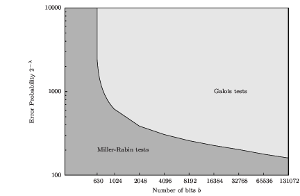
Figure 2. Ranges of efficiency for the Galois test

A reasonably optimized implementation in magma v2.18-2 is available on the authors’ web pages for independent checks. In order to see how practical is this implementation, we have picked a few random integers of sizes ranging from 1024 to 8192 bits, and we have measured the timings for those which turn to be pseudo-primes. As expected, the cost ratio between $\lambda/2$ Miller-Rabin tests and one equivalent Galois test increases with $b$. Results are collected in Table 1.

$$\begin{array}[]{|c|c|c|c|c||r|r|r|r|r|r|r||r|}\hline\cr\vrule\lx@intercol\hfil\mathrm{Parameters}\hfil\lx@intercol\vrule\lx@intercol\vrule\lx@intercol&\vrule\lx@intercol\hfil\mathrm{Galois}\hfil\lx@intercol\vrule\lx@intercol\vrule\lx@intercol&\mathrm{Miller-}\\ \cline{1-12}\cr b&\lambda&r&{d_{\rm cyc}}&{d_{\rm kum}}&2&4&5&9&\sigma(x)&x^{n}&\mathrm{Tot.}&\mathrm{Rabin}\\[2.84544pt] \hline\cr\hline\cr\hbox{\multirowsetup 1024}&\hbox{\multirowsetup 512}&129&1&15&0.0&0.3&-&0.0&0.0&0.2&0.5&\hbox{\multirowsetup 0.5}\\ &&171&2&6&0.0&0.4&0.0&0.0&0.0&0.3&0.7&\\ \hline\cr\hline\cr\hbox{\multirowsetup 2048}&\hbox{\multirowsetup 1024}&181&1&20&0.0&2.1&-&0.0&0.2&1.5&3.8&\hbox{\multirowsetup 6.2}\\ &&237&2&8&0.0&2.9&0.0&0.1&0.2&2.0&5.2&\\ \hline\cr\hline\cr\hbox{\multirowsetup 4096}&\hbox{\multirowsetup 2048}&246&1&28&0.0&18.7&-&0.0&1.3&11.6&31.6&\hbox{\multirowsetup 75.1}\\ &&293&2&12&0.0&22.6&0.0&1.0&1.9&19.8&45.3&\\ \hline\cr\hline\cr\hbox{\multirowsetup 8192}&\hbox{\multirowsetup 4096}&333&1&40&0.4&176.9&-&0.7&1.3&122.5&314.8&\hbox{\multirowsetup 1215.0}\\ &&424&2&16&0.4&251.6&0.2&5.3&18.8&198.3&474.6&\\ &&316&3&14&0.4&169.7&1.9&7.8&25.6&266.7&472.1&\\ \hline\cr\end{array}$$

Table 1. Compared timings for $b$-bit integers, and prob. up to $2^{-{b}/{2}}$ (in seconds)

References

- [1] Adleman, L.M., Pomerance, C., Rumely, R.S.: On distinguishing prime numbers from composite numbers. Ann. of Math. (2) 117(1), 173–206 (1983). DOI 10.2307/2006975. URL http://dx.doi.org/10.2307/2006975
- [2] Agrawal, M., Kayal, N., Saxena, N.: PRIMES is in P. Ann. of Math. (2) 160(2), 781–793 (2004). DOI 10.4007/annals.2004.160.781. URL http://dx.doi.org/10.4007/annals.2004.160.781
- [3] Auslander, M., Buchsbaum, D.: On ramification theory in Noetherian rings. Am. J. Math. 81, 749–765 (1959). DOI 10.2307/2372926
- [4] Avanzi, R.M., Mihăilescu, P.: Efficient quasi-deterministic primality test improving AKS URL http://www.math.uni-paderborn.de/~preda/
- [5] Bernstein, D.J.: Proving primality in essentially quartic random time. Math. Comp. 76(257), 389–403 (2007). DOI 10.1090/S0025-5718-06-01786-8. URL http://dx.doi.org/10.1090/S0025-5718-06-01786-8
- [6] Bourbaki, N.: Elements of mathematics. Commutative algebra. Hermann, Paris (1972). Translated from the French
- [7] Chase, S., Harrison, D., Rosenberg, A.: Galois theory and Galois cohomology of commutative rings. Mem. Am. Math. Soc. 52, 15–33 (1965)
- [8] DeMeyer, F., Ingraham, E.: Separable algebras over commutative rings. Lecture Notes in Mathematics, Vol. 181. Springer-Verlag, Berlin (1971)
- [9] Kedlaya, K.S., Umans, C.: Fast modular composition in any characteristic. In: FOCS, pp. 146–155. IEEE Computer Society (2008)
- [10] Lenstra, H.: Galois theory and primality testing. Universiteit van Amsterdam (1984). URL http://www.math.leidenuniv.nl/~hwl/PUBLICATIONS/pub.html
- [11] Lenstra, H.W.: Primality testing algorithms (after Adleman, Rumely and Williams). In: Séminaire Bourbaki, Vol. 1980/81, Lecture Notes in Math., vol. 901, pp. 243–257. Springer, Berlin (1981)
- [12] Lenstra, H.W., Pomerance, C.: Primality testing with gaussian periods URL http://www.math.dartmouth.edu/~carlp/PDF/complexity12.pdf
- [13] Miller, G.L.: Riemann’s hypothesis and tests for primality. J. Comput. System Sci. 13(3), 300–317 (1976). Working papers presented at the ACM-SIGACT Symposium on the Theory of Computing (Albuquerque, N.M., 1975)
- [14] Papadimitriou, C.M.: Computational complexity. Addison-Wesley, Reading, Massachusetts (1994)
- [15] Schoof, R.: Four primality testing algorithms. In: Algorithmic number theory: lattices, number fields, curves and cryptography, Math. Sci. Res. Inst. Publ., Surveys in Number Theory, vol. 44, pp. 101–126. Cambridge Univ. Press, Cambridge (2008)
- [16] Shoup, V.: Fast construction of irreducible polynomials over finite fields. J. Symbolic Comput. 17(5), 371–391 (1994). DOI 10.1006/jsco.1994.1025. URL http://dx.doi.org/10.1006/jsco.1994.1025