.

Coulomb potential

and the paradoxes of PT-symmetrization

Miloslav Znojil

Nuclear Physics Institute ASCR, 250 68 Řež, Czech Republic,

e-mail: znojil@ujf.cas.cz

Abstract

Besides the standard quantum version of the Coulomb/Kepler problem, an alternative quantum model with not too dissimilar phenomenological (i.e., spectral and scattering) as well as mathematical (i.e., exact-solvability) properties may be formulated and solved. Several aspects of this model are described. The paper is made self-contained by explaining the underlying innovative quantization strategy which assigns an entirely new role to symmetries.

1 Introduction

The list of the traditional roles of symmetries in Quantum Theory has recently been enriched by the increasingly active studies of the role of the so called ${\cal PT}-$symmetries [1]. Typically, one considers a Hamiltonian composed of a kinetic- and potential-energy terms,

$$H=-\frac{\ \hbar^{2}}{2m}\,\triangle+V(x)$$

and replaces the current requirement $H=H^{\dagger}$ of its Hermiticity in Hilbert space $L^{2}(\mathbb{R}^{d}):={\cal H}^{(friendly)}$ by the less trivial physical Hermiticity (or rather “crypto-Hermiticity” [2]) $H=H^{\ddagger}$ which must be constructively, ad hoc defined in another Hilbert space ${\cal H}^{(standard)}$. In the language of symmetries this means that, firstly, the “usual” Hermiticity $H=H^{\dagger}$ is reinterpreted as a formal time-reversal symmetry

$$H\,{\cal T}={\cal T}\,H$$ (1)

(with a suitable time-reversal operator ${\cal T}$). In the second step one rejects the constraint (1) as “too formal” [3] and postulates, instead, the Hermiticity of $H=H^{*}$ in an auxiliary Krein space with a suitable indefinite pseudometric ${\cal P}$. In other words, in the language of symmetries one follows the recommendations of mathematicians [4, 5] and re-facilitates the mathematics by the replacement of Eq.  (1) by the modified requirement called ${\cal PT}$ symmetry,

$${\cal PT}\,H=H\,{\cal PT}\,.$$ (2)

In the context of physics the recipe finds its most ambitious theoretical encouragement in the appeal of the concept of such a form of symmetry in relativistic quantum field theory [6], with ${\cal P}$ representing the parity and with ${\cal T}$ mimicking the time reversal in this implementation.

Another explanation of the increasing popularity of the whole concept certainly lies in the amazing productivity of the ${\cal PT}-$symmetrizations of various quantum systems. In the popularization of such a trick the key role has been played by the serendipitious letter [7] in which Bender and Boettcher proposed and demonstrated that the ${\cal PT}-$symmetrization of a given local Schrödinger equation in single dimension (i.e., a transition from constraint (1) to constraint (2) at $d=1$) may represent an efficient theoretical tool and way towards finding new phenomenologically useful Hamiltonians with real spectra. They also recommended to achieve this simply by the replacement of the original Hermitian potential $V(x)$ by its non-Hermitian alternative $V({\rm i}x)$ (thorough review offered by paper [3] may be recommended as an introductory reading).

In our present paper we intend to return to the older application of this idea to the exactly solvable Coulomb/Kepler problem [8] and to its recent upgrades [9] – [11]. We intend to review the related recent theoretical developments and to show how the incessant progress in the field applies to this particular but important example.

2 The ${\cal PT}-$symmetric version of the Coulomb problem

In loc. cit., the standard quantum Coulomb/Kepler problem has been assigned a new, non-equivalent quantum system version which is formally represented by the ${\cal PT}-$symmetric Schrödinger equation

$$\frac{\ \hbar^{2}}{2m}\,\left[-\frac{{\rm d}^{2}}{{\rm d}{x}^{2}}+\frac{L(L+1)}{{x}^{2}}\right]\,\Psi({x})+\frac{{\rm i}Z}{x}\,\Psi({x})=E\,\Psi({x})\,,\ \ \ L>-\frac{1}{2}\,,\ \ \ \ 2L\ \notin\mathbb{Z}\,.$$ (3)

We shall abbreviate here $2mE/\hbar^{2}=-k^{2}$ and emphasize that even in the presence of the imaginary unit, this equation remains solvable in terms of the well known confluent hypergeometric functions,

$$\Psi_{1}(x)=C_{1}\Psi_{1}(x)+C_{2}\Psi_{2}(x)\,,$$ (4)

$$\Psi_{1}(x)=e^{-kx}x^{L+1}{{}_{1}}{F}{{}_{1}}(1+L+{{\rm i}Z}/{(2k)},2L+2,2kx)\,,$$ (5)

$$\Psi_{2}(x)=e^{-kx}x^{-L}{{}_{1}}{F}{{}_{1}}(-L+{{\rm i}Z}/{(2k)},-2L,2kx)\,.$$ (6)

The well known Coulomb – harmonic oscillator correspondence has been studied in [8]. In the role of a formal postulate it helped us to fix the physical asymptotic boundary conditions which would remain, otherwise, ambiguous (Ref. [12] and previous loci citati should be consulted for all details).

It has been shown [13] that all of the models of the class sampled by Eqs. (3) + (4) may be perceived, under certain conditions which we explained in Ref. [2], as fully compatible with the standard postulates of Quantum Mechanics.

Our present paper will expose Eq. (3) as a special case of the broader class of Schrödinger equations which all exemplify an extension of quantum model-building strategies. In Ref. [2] we called this approach a “crypto-Hermitian” or “three-Hilbert-space” quantum mechanics. We shall emphasize here that the transition from the Hermitian to ${\cal PT}-$symmetric language is extremely productive while, at the same time, its multistep nature often leads to conceptual misunderstandings. While “teaching by example”, we shall try to clarify here some of the most blatant ones.

3 The abstract formalism

Several compact review papers [3, 2, 14] may be recommended for reference. At the same time, an introductory explanation of the structure of Quantum Mechanics using the pseudometric in Krein space may be given, for our present purposes, a much shorter form.

First of all the readers should be warned that in the majority of textbooks on Quantum Mechanics the meaning of the Dirac-ket symbols $|\psi\rangle\in{\cal V}$ is merely explained via examples. Most often one deals just with the most common quantum motion of a point particle inside a local potential well. Thus, it is assumed that there exists an operator $\hat{Q}$ of the particle position with eigenvalues $q\in\mathbb{R}^{d}$ and eigenkets $|q\rangle$. The standard (often called Dirac’s) Hermitian conjugation is then represented by the transposition plus complex conjugation of any ket vector, yielding the bra vector,

$${\cal T}^{(Dirac)}:|\psi\rangle\ \to\ \langle\psi|\,.$$ (7)

In the basis $|q\rangle$ one may then represent the ket of any pre-prepared state $|\psi\rangle$ by the overlap $\psi(q)=\langle q|\psi\rangle$, i.e., by the square-integrable wave function of the coordinate $q$.

Our present purpose is not a criticism of this approach as such (interested readers may find such a criticism elsewhere [15]) but rather just of one of its consequences. In virtually all of the similar classes of examples, indeed, the vector space of states ${\cal V}$ is simply assumed endowed with the most common inner product

$$\langle\psi_{a}|\psi_{b}\rangle=\int_{-\infty}^{\infty}\,\psi_{a}^{*}(q)\psi_{b}(q)\ dq$$ (8)

with, possibly, the integration replaced by the infinite or finite summation. Thus, we may (and usually do) set ${\cal V}\equiv L^{2}(\mathbb{R})$, etc.

Without any real danger of misunderstanding we may speak here about the “friendly” Hilbert space of states ${\cal H}^{(F)}\equiv{\cal V}$, calling the variable $q$ in Eq. (8) “the coordinate”. In parallel we usually perform a maximally convenient choice of the Hamiltonian $H$ based on the so called principle of correspondence which encourages us to split the Hamiltonian into the kinetic and potential energies, $H=T+V$. Whenever the general interaction operator $V$ is represented, say, by a kernel $V(q,q^{\prime})$ when acting upon the wave functions, this kernel is most often chosen as proportional to the Dirac’s delta-function so that $V$ becomes an elementary multiplicative operator $V=V_{local}=V(q)$. Similarly, the most popular and preferred form of the “kinetic energy” $T$ is a differential operator, say, $T=T_{local}=-d^{2}/dq^{2}$ in single dimension and in the suitable units.

The word of strong warning emerges when we perform a Fourier transformation in ${\cal H}^{(F)}$ so that the variable $q$ becomes replaced by $p$ (= momentum). One should rather denote the latter, Fourier-image space by the slightly different symbol ${\cal H}^{(P)}$, therefore (with the superscript still abbreviating “physical” [2]).

Paradoxically, after the latter change of frame the kinetic operator $T_{local}$ becomes multiplicative while $V_{local}$ becomes strongly non-local in momenta. Nevertheless, all this does not modify the overall paradigm. A truly deep change of the paradigm only comes with the models where the necessity of the observability of the coordinate $q$ is abandoned completely. One may still start from the vector space of kets ${\cal V}$ but it makes sense to endow it with another Hilbert-space structure, via the inner product defined by an integral over a complex path,

$$\langle\psi_{a}|\psi_{b}\rangle=\int_{\cal C}\,\psi_{a}^{*}(s)\psi_{b}(s)\ ds\,.$$ (9)

This is one of the most characteristic intermediate steps made in the so called ${\cal PT}-$symmetric quantum theories [3]. The resulting loss of simplicity of the position operator $\hat{Q}$ changes the physics of course. The key point is that we lose the one-to-one correspondence between the integration path ${\cal C}$ and the spectrum $\mathbb{R}$ of any coordinate-mimicking operator. The physics-independent optional variable $s$ becomes purely formal.

In such a setting our choice of the physical observables must still obey the old quantization paradigm, which is just set in a modified context. The loss of the observability of the coordinate proves essential, anyhow. For illustration one might recall the pedagogically motivated paper [16] in which, in a slightly provocative demonstration of the abstract nature of quantum theory, the variable $s$ in Eq. (9) has been interpreted as an observable “time” of a hypothetical “quantum clock” system.

Once we wish to understand our Coulombic Schrödinger eigenvalue problem (3), we must make one more step and generalize further the inner products (9). Such a second-step generalization of the inner product will certainly move us from the two Hilbert spaces ${\cal H}^{(F)}$ and ${\cal H}^{(P)}$ to the third one, viz., to the final and physical “standard” Hilbert space ${\cal H}^{(S)}$ (this notation is taken from Ref. [2]).

The introduction of the third Hilbert space forms the theoretical background of an amendment of the traditional quantum mechanics, the key nonstandard features of which can be seen

• in the admissibility of the complex potentials sampled by the power-law-anharmonic family $V(s)=-({\rm i}s)^{2+\delta}$ of Ref. [7] and generating the real and discrete bound-state spectra at any $\delta>0$ (cf. the proofs in [17]);

• in the replacement of the usual real line of $s$ by a complex curve ${\cal C}=\mathbb{C}(\mathbb{R})$ which may even be, in principle, living on a complicated multisheeted Riemann surface [12];

• in the theoretical imperative of the construction of certain operator $\Theta$ (see below);

• in the possibility of a systematic study of the discretizations and simplifications.

In our present paper, the emphasis will be put on the last feature.

At the stage of development where we did not yet explain the meaning and role of the operator $\Theta$ (called Hilbert space metric) the theory remains incomplete. We already cannot rely upon a more or less safe guidance of quantization as offered by the principle of correspondence. Just a partial revitalization of such guidance is possible in the new context (cf., e.g., a nice example-based discussion of this point in Ref. [13]).

This being said, the main theoretical obstacle lies in the vast ambiguity of the necessary appropriate generalization of the Hermitian conjugation as prescribed by Eq. (7). The general recipe (explained already in [18] or, more explicitly, in [2]) is $\Theta-$dependent and reads

$${\cal T}^{(general)}_{\Theta}:|\psi\rangle\ \to\ \langle\!\langle\psi|:=\langle\psi|\Theta\,.$$ (10)

This means that using the language of wave functions $\psi(s)$ with $s\in{\cal C}$ we must replace the most common single-integral definition (9) of the inner product in the original “friendly” Hilbert space ${\cal H}^{(F)}$ by the more sophisticated double-integral formula

$$\langle\!\langle\psi_{a}|\psi_{b}\rangle=\int_{\cal C}\,\int_{\cal C}\,\psi_{a}^{*}(s)\,\Theta(s,s^{\prime})\,\psi_{b}(s^{\prime})\ ds\,ds^{\prime}\,.$$ (11)

In terms of an integral-operator-kernel representation $\Theta(s,s^{\prime})$ of our abstract metric operator $\Theta=\Theta^{\dagger}>0$ this recipe defines the inner product which converts the same ket-vector space ${\cal V}$ into the amended and final, metric-dependent and physics-representing Hilbert space ${\cal H}^{(S)}$ of the very standard quantum theory (cf. [2] for more details).

4 The upgraded formalism in applications

In the attempted applications of all of the new ideas to the traditional benchmark models like Coulomb scattering one may make use of its traditional merits (like, e.g., exact solvability) as well as of the flexibility of the choice of the ${\cal PT}-$symmetric (i.e., complex and left-right symmetric) integration path, sampled in Ref. [10] as follows,

$$x(s)=x^{U}_{(\varepsilon)}(s)\,=\,\left\{\begin{array}[]{ll}-{\rm i}(s+\frac{\pi}{2}\varepsilon)-\varepsilon,&s\in(-\infty,-\frac{\pi}{2}\varepsilon),\\ \varepsilon e^{{\rm i}({s/\varepsilon+3/2\pi})},&s\in(-\frac{\pi}{2}\varepsilon,\frac{\pi}{2}\varepsilon),\\ {\rm i}(s-\frac{\pi}{2}\varepsilon)+\varepsilon\,,&s\in(\frac{\pi}{2}\varepsilon,\infty).\end{array}\right.$$ (12)

This leads to new results of course. Typically, in spite of the non-unitarity of the scattering (remember that the Coulomb potential is strictly local!) the bound-state energies still emerge from the poles of the scattering matrix [10].

4.1 Discretizations

The use of discretizations of the differential forms of Schrödinger operators may be, typically, Runge-Kutta-inspired. In practice, they are slowly becoming useful in solid-state physics [19], optics [20] and statistical physics [21]. Less expectedly, the use of lattice models proved crucial for the unitarity of the scattering. It has been shown [22] that the theory of scattering by non-Hermitian obstacles may be made unitary and consistent via a certain selfconsistently prepared transition to non-local potentials. Unfortunately, it is not yet clear how such a requirement of selfconsistency could be realized in the continuous limit of the discrete models.

Whenever we discretize the coordinates and replace the differential Hamiltonians by matrices with property $H\neq H^{\dagger}$, the above-reviewed theory applies without changes. The usual Hilbert space becomes unphysical and it must be replaced by its unitarily non-equivalent correct alternative ${\cal H}^{(S)}$ endowed with a sophisticated metric $\Theta=\Theta^{(S)}\neq I$ which defines the ad hoc inner product.

In the discretized version of the theory, the integral kernel of the metric must merely be replaced by a matrix. Naturally, also the double integral (11) gets replaced by the double sum,

$$(\psi,\phi)^{(S)}=\sum_{j,k=1}^{N}\,\psi^{*}_{j}\,\Theta_{j,k}^{(S)}\,\phi_{k}\$$

in ${\cal H}^{(S)}$. In this setting, the imaginary choice of the Coulomb coupling may still be made compatible with the standard postulates of Quantum Theory, provided only that it still generates the real, i.e., potentially observable spectrum of the bound-state energies.

Once we started our considerations from the imaginary Coulomb model defined along a continuous complex trajectory, we may expect that many of its properties will survive also the transition to its discrete descendants. For inspiration we may recall Ref. [10] where the bound-state energies were shown to coincide with the poles of transmission coefficients. Still, as long as the potential $V\neq V^{\dagger}$ is local, the unitarity of the scattering cannot be required [10, 22]. At the same time, the unitarity of the time evolution of the system itself may be achieved. Indeed, although the Hamiltonian $H$ is non-Hermitian in ${\cal H}^{(F)}$, (abbreviated $H\neq H^{\dagger}$), it is Hermitian in ${\cal H}^{(S)}$. This feature is called cryptohermiticity, requiring $H=H^{\ddagger}$ alias

$$H^{\dagger}\Theta^{(S)}=\Theta^{(S)}\,H\,.$$

Here, the operator or matrix $\Theta^{(S)}$ is precisely the one which defines the physical inner product.

This being said, the loss of easy constructions is a problem [23]. Still, the discretization of the coordinates may be recommended as the recipe.

4.2 Interpretations

The generic ${\cal PT}-$ symmetric quantum model describes a closed system defined via a doublet of operators $\ {H,\Theta}\$ or via a triplet of operators (adding a new observable $\Lambda$ and having, typically, Hamiltonian $H\neq H^{\dagger}$ accompanied by a charge [3]), etc. In other words, the dynamical content of phenomenological quantum models is encoded in Hamiltonian $H$ and in metric $\Theta$. In this setting the metric $\Theta$ guarantees the unitarity of time evolution in an ad hoc, “standard” Hilbert space [18], to be denoted by the symbol ${\cal H}^{(S)}$ in what follows. In addition, one can also impose some other, phenomenologically motivated requirements like a short-range smearing of coordinates [24], etc.

One of the remarkable features of such an upgrade of applications of quantum mechanics may be seen in the robust nature of its “first principles” which remain unchanged. Thus, its traditional probabilistic interpretation is not changed (notice that it practically did not change during the last cca eighty years!). In the language of textbooks one could speak just about the use of a non-unitary generalizations $\Omega\sim\sqrt{\Theta}$ of the most common Fourier transformations. Still, the new physics behind the trick may be nontrivial (in nuclear physics, for example, the mapping $\Omega$ (called Dyson’s [18]) was used to represent fermions as images of bosons).

Among the most innovative consequences of the upgraded formulation of quantum models one notices, first of all, the existence and possibility of constructions of a horizon [25]. Formally, this notion coincides with the set $\partial{\cal D}$ of the Kato’s [26] exceptional points in the (real or complex) manifold ${\cal D}$ of available free parameters (like coupling strengths, etc). The practical appeal of this notion may be based, e.g., on its tunability [27] and/or a new physics near instabilities and quantum catastrophes [28].

As another emergent concept one should list fundamental length, i.e., a quantity $\theta$ defined, in the simplified discrete models, as the number of diagonals in the metric which is required to possess a band-matrix form, $\Theta^{(S)}_{mn}=0\ {\rm for}\ |m-n|>\theta$. In this context one might mention the first papers devoted to the study of ${\cal PT}-$symmetric quantum graphs [29] in which one might search for a connection between the fragile parts of the spectrum and the topological characteristics of the underlying graph structure.

Last but not least, it is necessary to emphasize the challenging character of a generic scenario with more observables, each of which may be responsible for its own part of the physical horizon, “invisible” from the point of view of the other observables. In other words, a lot of work is still to be done before one could speak about a “classification” of exceptional points (i.e., about a a sort of “quantum theory of catastrophes”) – the first attempts in this direction only dealt with the hardly realistic, too oversimplified and schematic quantum systems [30].

5 Coulomb potential $V(x_{j})={\rm i}/x_{j}$

The main weak point of the above-cited choice of the Coulomb potential may be identified not only with its strict locality (i.e., with the necessary loss of the unitarity of the scattering, cf. also the detailed study [23] in this respect) but also with the difficulties encountered during transition to any model which would not be exactly solvable. For this reason, our present use of the Runge-Kutta-inspired discretization will help also in the case of the Coulomb potential.

As long as our present main ambition is the presentation of the upgraded formalism, we shall try to simplify many inessential mathematical aspects of our Coulomb/Kepler model. In parallel, we shall also try to treat this potential as a special case of a broader class of forces. For the sake of definitness and in a way insspired by Ref. [annalso], we shall pick up the class $V(x)={\rm i}x^{z}$ with a real exponent which does not lie too far from its Coulombic value of $z=-1$.

For this purpose we must replace, first of all, the typical differential Schrödinger equation

$$-\frac{d^{2}}{dx^{2}}\,\psi_{n}(x)+V(x)\,\psi(x)=E_{n}\,\psi_{n}(x)\,\ \ \ \ \ \ \ \psi(\pm\Lambda)=0\,,\ \ \ \ 1\ll\Lambda\leq\infty$$ (13)

by its discrete version (i.e., approximation or analogue)

$$-\frac{\psi(x_{k-1})-2\,\psi(x_{k})+\psi(x_{k+1})}{h^{2}}+V(x_{k})\,\psi(x_{k})=E\,\psi(x_{k})\,.$$ (14)

An equidistant grid of the Runge-Kutta points $x_{k}=-\Lambda+k\,h$ with $k=0,1,\ldots,N+1$ will be used. In this sense, also the standard general double-integral inner product will be replaced by the above-mentioned double sum, etc.

Naturally, the discretization recipe also involves the change of the asymptotic boundary conditions, with $x_{N+1}=\Lambda$, $h=2\Lambda/(N+1)$ and $\psi(x_{0})=\psi(x_{N+1})=0$. In other words, the eigenvalue calculations become reduced to the mere diagonalizations of the $N$ by $N$ matrix Hamiltonians

$${H}^{(N)}=\left(\begin{array}[]{ccccc}2+h^{2}V(x_{1})&-1&&&\\ -1&2+h^{2}V(x_{2})&-1&&\\ &-1&2+h^{2}V(x_{3})&\ddots&\\ &&\ddots&\ddots&-1\\ &&&-1&2+h^{2}V(x_{N})\end{array}\right)\,.$$ (15)

The insertion of any potential $V(x_{j})={\rm i}x_{j}^{z}$ will lead to the eigenvalues $\varepsilon_{j}:=h^{2}E^{(N)}_{j}\in(0,4)$ which must be computed numerically in general.

In some applications the transition to the continuous limit $N=\infty$ is made or, at worst, postponed till the end of the calculations. In the present methodical context we shall rather keep the dimension $N$ constant and, in fact, not too large.

The insertion of formula $V(x_{j})={\rm i}/x_{j}$ in Eq. (15) with even $N=2K$ yields the sequence of the discrete ${\cal PT}-$symmetric Coulomb Hamiltonians $H^{(2K)}(a)=$

$$\left[\begin{array}[]{cccccccc}2-i\,a\,/(2K-1)&-1&0&\ldots&&&\ldots&0\\ -1&\ddots&\ddots&\ddots&&&&\vdots\\ 0&\ddots&2-i\,a\,/3&-1&0&&&\\ \vskip 6.0pt plus 2.0pt minus 2.0pt\cr\vdots&\ddots&-1&2-ia&-1&0&&\\ \vskip 6.0pt plus 2.0pt minus 2.0pt\cr&&0&-1&2+ia&-1&\ddots&\vdots\\ \vskip 6.0pt plus 2.0pt minus 2.0pt\cr&&&0&-1&2+i\,a\,/3&\ddots&0\\ \vdots&&&&\ddots&\ddots&\ddots&-1\\ \vskip 6.0pt plus 2.0pt minus 2.0pt\cr 0&\ldots&&&\ldots&0&-1&2+i\,a\,/(2K-1)\end{array}\right]\,.$$ (16)

In its first nontrivial example let us set $N=4$,

$$H^{(4)}(a,z)=\left[\begin{array}[]{cccc}2-i\,a\,3^{z}&-1&0&0\\ \vskip 6.0pt plus 2.0pt minus 2.0pt\cr-1&2-ia&-1&0\\ \vskip 6.0pt plus 2.0pt minus 2.0pt\cr 0&-1&2+ia&-1\\ \vskip 6.0pt plus 2.0pt minus 2.0pt\cr 0&0&-1&2+i\,a\,3^{z}\end{array}\right]\,,\ \ \ \ z=-1\,.$$ (17)

We see that a natural generalization may be targeted not only at the growing dimensions $N>4$ but also towards the small deviations of the exponent $z$ from its Coulombic value. Empirically, one can verify that in both of these directions, the spectral loci (i.e., eigenvalues $\varepsilon^{(N,z)}(a)$) remain topologically the same. More precisely, at a fixed $N$, the topology of the Coulomb-potential pattern as sampled by Figs. 1 - 3 may be expected to survive all the negative exponents $z$ [11].

At $N=4$ the model is exactly solvable at the Coulombic exponent $z=-1$. The secular equation

$${{\it{E}}}^{4}-8\,{{\it{E}}}^{3}+\left(21+{\frac{10}{9}}\,{a}^{2}\right){{\it{E}}}^{2}+\left(-{\frac{40}{9}}\,{a}^{2}-20\right){\it{E}}+5+1/9\,{a}^{4}+5\,{a}^{2}=0$$

generates the closed-form spectrum

$$\varepsilon(a)=2\pm 1/6\,\sqrt{54-20\,{a}^{2}\pm 2\,\sqrt{405-720\,{a}^{2}+64\,{a}^{4}}}\,,$$

which is real iff $|a|\leq 3/4\,\sqrt{10-4\,\sqrt{5}}\approx 0.7706147226$.

At $N=6$ the model is still exactly solvable at $z=-1$, yielding the secular equation

$${{\it{E}}}^{6}-12\,{{\it{E}}}^{5}+\left(55+{\frac{259}{225}}\,{a}^{2}\right){{\it{E}}}^{4}+\left(-120-{\frac{2072}{225}}\,{a}^{2}\right){{\it{E}}}^{3}+$$

$$+\left(126+{\frac{5894}{225}}\,{a}^{2}+{\frac{7}{45}}\,{a}^{4}\right){{\it{E}}}^{2}+\left(-56-{\frac{280}{9}}\,{a}^{2}-{\frac{28}{45}}\,{a}^{4}\right){\it{E}}+$$

$$+7+14\,{a}^{2}+{\frac{7}{9}}\,{a}^{4}+{\frac{1}{225}}\,{a}^{6}=0$$

which may be solved using Cardano formulae. Although the closed form of the spectrum becomes extremely clumsy in this representation, it decisively facilitates the graphical representation of the spectral loci which all appear topologically equivalent to the vertical array of circles. In particular, the survival of the exact solvability of the problem enables us to conclude that the whole $N=6$ spectrum remains real iff $|a|\leq 0.589586$.

These results indicate that the topological pattern remains generic and $N-$independent. Such a conjecture is persuasively confirmed by the larger$-N$ graphical samples which are presented in Figs. 2 and 3.

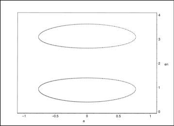
Figure 1: The $a-$dependence of energies $\varepsilon(a)$ at $N=4$.

5.1 Graphical methods

Numerical evaluation of the spectra is sampled in Figs. 1, 2 and 3. These graphical constructions indicate that at any $N=2K$ the spectrum is real iff $a\in\left(-\alpha^{(2K)},\alpha^{(2K)}\right)$ and fully complex for $a\notin\left(-\beta^{(2K)},\beta^{(2K)}\right)$. where $\alpha^{(2K)}$ is a quickly decreasing function of $K$.

The latter observation may be interpreted in two ways. For the finite lattices in which the numerical value of parameter $a$ is fixed, the reality of the spectrum is, undoubtedly, fragile. In the alternative approach in which our model serves just as a simulation of the (NB: exactly solvable!) differential-equation system, the definition of parameter $a$ is prescribed by the Runge-Kutta recipe (see above). For this reason, its numerical value decreases, with $N$, much more quickly than $\alpha^{(N)}$. This implies that in the latter setting the reality of the spectrum may be declared robust and guaranteed.

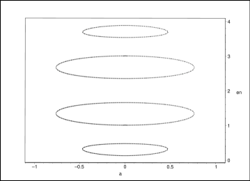
Figure 2: The $a-$dependence of energies $\varepsilon(a)$ at $N=8$.

Marginally, we may add that in the former scenario using small and fixed $N$, the loss of the reality of the spectrum is caused by the confluence of the ground state with the first excited state and by their subsequent complexification. Due to the up-down symmetry of the spectrum, this instability is paralleled by the upper two states of course.

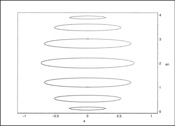
Figure 3: The $a-$dependence of energies $\varepsilon(a)$ at $N=14$.

6 Hermitizations

6.1 The $N=2$ metrics

The condition of hidden Hermiticity of any Hamiltonian with real spectrum is often called Dieudonné equation [2],

$$H^{(N)}=\left[H^{(N)}\right]^{\ddagger}:=\Theta^{-1}\left[H^{(N)}\right]^{\dagger}\Theta\,.$$ (18)

Its structure is best illustrated at $N=2$ where the metrics form just the two-parametric family

$$\Theta\left[H^{(N)}(a)\right]=\Theta\left[H^{(N)}(a)\right]_{(k,m)}=\left[\begin{array}[]{cc}k&km-ika\\ \vskip 6.0pt plus 2.0pt minus 2.0pt\cr km+ika&k\end{array}\right]\,,\ \ k,m\in\mathbb{R}\,.$$ (19)

With the condition $a\in(-1,1)$ of the reality of energies and with the metric-positivity constraint

$$\theta=\theta_{\pm}=k\pm\sqrt{{k^{2}m}^{2}+{k}^{2}{a}^{2}}>0\,$$ (20)

we may conclude that $k$ must be positive and larger than the square root. We may reparametrize $a=\cos\beta\,\sin\gamma$, $m=\cos\beta\,\cos\gamma$, $\beta\in(0,\pi)$ and $\gamma\in(0,\pi)$ and $-1<\cos\beta<1$ and get the final result

$$\Theta=\Theta\left\{H^{(2)}[a(\beta,\gamma)]\right\}_{[k,m(\beta,\gamma)]}=k\cdot\left[\begin{array}[]{cc}1&e^{-{\rm i}\gamma}\cos\beta\\ \vskip 6.0pt plus 2.0pt minus 2.0pt\cr e^{{\rm i}\gamma}\cos\beta&1\end{array}\right]\,.$$ (21)

In a search for the other eligible observables with crypto-Hermiticity property

$$\Lambda_{(\beta,\gamma)}^{\dagger}\,\Theta_{[k,m(\beta,\gamma)]}=\Theta_{[k,m(\beta,\gamma)]}\,\Lambda_{(\beta,\gamma)}\,.$$ (22)

the use of the ansatz

$$\Lambda=\left[\begin{array}[]{cc}G+{\rm i}g&B+{\rm i}b\\ \vskip 6.0pt plus 2.0pt minus 2.0pt\cr C+{\rm i}c&D+{\rm i}d\end{array}\right]\,.$$ (23)

leads to the four real constraints imposed upon eight free parameters. The family of observables is four-parametric, therefore. Three constraints define $B$, $C$ and $G-D$. The remaining one relates the sums $c_{\Sigma}=b+c$ and $g_{\Sigma}=g+d$ and leads to the unique solution $g_{\Sigma}=0$. We may conclude that from the input $m=m(\beta,\gamma)$ and $a=a(\beta,\gamma)$ one gets the class of admissible observables

$$\Lambda=\Lambda(D,b,c,g)=\frac{1}{a}\cdot\left[\begin{array}[]{cc}D\,a-b-c+i\,g\,{a}\,,&g-b\,m+i\,b\,a\\ \vskip 6.0pt plus 2.0pt minus 2.0pt\cr{g+c\,m}+i\,c\,a\,,&D\,a-i\,g\,a\end{array}\right]\,.$$ (24)

In particular, the initial Hamiltonian is reobtained at $D=2$, $G=2$, $b=c=0$, $B=C=-1$ and $g=-a\ (=-d)$.

In the literature the concept of charge is considered particularly useful [3]. Its essence lies, in the present model, in an additional auxiliary assumption

$$\left[H\right]^{\dagger}{\cal P}={\cal P}\,H\,$$ (25)

where ${\cal P}$ is the operator of parity. Under this assumption a unique metric is sought such that a very specific metric called ${\cal CPT}$ metric is prescribed by formula $\Theta^{({\cal CPT})}={\cal CP}$ where ${\cal C}$ is called “charge”.

Thus, at a given $N$ we may define the parity ${\cal P}={\cal P}^{(N)}$ which contains units along the secondary diagonal, i.e., ${\cal P}^{(N)}_{m,n}=1$ iff $m+n=N+1$ while ${\cal P}^{(N)}_{m,n}=0$ otherwise. Incidentally one may note that ${\cal P}^{(2)}$ = limit of $\Theta\left[H^{(2)}(a)\right]$ such that $k^{({\cal P})}\to 0$, $m^{({\cal P})}\to\infty$, $k^{({\cal P})}m^{({\cal P})}\to 1$.

The key merit of the use of charge is that its use makes the metric unique,

$${\cal C}^{({\cal CPT})}=k\cdot\left[\begin{array}[]{cc}-{\rm i}a&1\\ \vskip 6.0pt plus 2.0pt minus 2.0pt\cr 1&{\rm i}a\end{array}\right]\,.$$ (26)

Moreover, it also represents one of the special cases of observable $\Lambda$ using $D=b=c=0$ and $g=-\cos\beta/\sin\beta=-\sqrt{k^{2}-1}$. Indeed, from $\Theta^{({\cal CPT})}={\cal CP}$ we have

$${\cal C}=\Theta\left[H^{(2)}(a)\right]_{(k,m)}{\cal P}^{(2)}=\left[\begin{array}[]{cc}u&v\\ \vskip 6.0pt plus 2.0pt minus 2.0pt\cr y&z\end{array}\right]\,$$ (27)

yielding $v=y=k$ and $z=u^{*}=ke^{i\gamma}\cos\beta$. Then, condition ${\cal C}^{2}=I$ requires that $\gamma=\gamma^{({\cal CPT})}=\pi/2$ (i.e., $a=\cos\beta$). Thus, we have $\beta=\beta^{({\cal CPT})}$ such that $\sin\beta^{({\cal CPT})}=1/k$. This proves the above statement.

6.2 The $N=4$ metrics

With the natural ansatz for $\Theta\left[H^{(4)}(a,z)\right]_{(k,m,r,h)}=$

$$=\left[\begin{array}[]{cccc}k&m-ikw&W^{*}&Z^{*}\\ \vskip 6.0pt plus 2.0pt minus 2.0pt\cr m+ikw&r&h-i\left(kw+ra\right)&W^{*}\\ \vskip 6.0pt plus 2.0pt minus 2.0pt\cr W&h+i\left(kw+ra\right)&r&m-ikw\\ \vskip 6.0pt plus 2.0pt minus 2.0pt\cr Z&W&m+ikw&k\end{array}\right]$$ (28)

where $w=w(z,a)={3}^{z}{a}\$ and

$$W=W(k,m,r)=-{w}^{2}k+r-k-kwa+i\left(wm+ma\right)\,,$$

$$Z=Z(k,m,r,h)=m{a}^{2}-{w}^{2}m-m+h-i\left(kw-ka-kw{a}^{2}-rw+{w}^{3}k\right)\,,$$

the problem of the determination of the domain of positivity of the metric starts to be merely tractable graphically.

For the numerous practical purposes the metric is sought in a special form. One of the phenomenologically inspired options is the choice of the matrix with units along its main diagonal, $k=r=1$. In addition, let us select $m=h=0$ and compute $W(1,0,1)=-{w}\left(w+a\right)$, $Z(1,0,1,0)=i\left(a+w{a}^{2}-{w}^{3}\right)$. Such a restricet construction leads to the following four closed-form eigenvalues of the metric $\Theta\left[H^{(4)}(a,z)\right]_{(1,0,1,0)}$, viz,

$$\theta_{+}^{\pm}=1+\frac{1}{2}\,\left(w-{a}^{2}w+{w}^{3}\right)\pm\frac{1}{2}\,\sqrt{\triangle^{+}}$$

$$\theta_{-}^{\pm}=1-\frac{1}{2}\,\left(w-{a}^{2}w+{w}^{3}\right)\pm\frac{1}{2}\,\sqrt{\triangle^{-}}$$

$$\triangle^{\pm}={w}^{6}+\left(2-2\,{a}^{2}\right){w}^{4}+\left(\pm 8+4\,a\right){w}^{3}+\left(5\pm 8\,a+6\,{a}^{2}+{a}^{4}\right){w}^{2}+$$

$$+\left(4\,a+4\,{a}^{3}\right)w+4\,{a}^{2}\,.\ \ \ \ \ \ \ \ \ \ \ \ \ \ \ \ \ \ \ \ \ \ \ \ \ \ \ \ \ \ \ \ \ \ \ \ \ \ \ \ \ \$$

Some details and numerical results of its analysis may be found elsewhere [11].

7 Discussion

In a climax of our present discussion of the discrete ${\cal PT}-$symmetric Coulomb problem characterized by the purely imaginary coupling constant, let us now summarize the overall method via the following scheme

$$\begin{array}[]{c}\begin{array}[]{|c|}\hline\cr\ {\rm textbook\ level\ quantum\ theory:}\\ {\rm{}prohibitively\ complicated}\ {\rm\ Hamiltonian}\ \mathfrak{h}\\ {\rm generating\ unitary\ time\ evolution}\\ \ \ \ \ {\rm\framebox{P:}\ {{}physics\ =\ trivial}}\\ \ \ \ \ \framebox{\rm calculations\ =\ practically\ impossible\ }\\ \hline\cr\end{array}\\ \stackrel{{\scriptstyle{}simplif\/ication}}{{}}\ \ \ \ \swarrow\ \ \ \ \ \ \ \ \ \ \ \ \ \ \ \ \ \ \ \ \ \ \ \ \ \ \ \ \ \ \ \searrow\nwarrow\ \ \ \stackrel{{\scriptstyle{}unitary\ equivalence}}{{}}\\ \begin{array}[]{|c|}\hline\cr\ {\rm\ state}\ \psi\ {\rm is\ represented}\\ \ {\rm in\ the}\ \framebox{{} false\ {\rm Hilbert\ space}}\\ \ {\rm\framebox{F:}\ calculations\ =\ {{}feasible}}\\ \ {\rm physical\ meaning\ =\ lost}\\ \ \ \ \ H={\rm non-Hermitian}\\ \hline\cr\end{array}\stackrel{{\scriptstyle{{}hermitization}}}{{\longrightarrow}}\begin{array}[]{|c|}\hline\cr\ \framebox{\rm amended \ inner\ product}\\ \ {\rm{}standardized}{\rm\ representation}\\ \ \ {\rm\framebox{S:}\ picture\ }=\ {\rm{}synthesis}\\ \ \ {\rm physics\ =\ reinstalled}\\ \ \ \ \ H={\rm Hermitian}\\ \hline\cr\end{array}\\ \\ \end{array}$$

which characterizes the “three-Hilbert-space” pattern of quantization as described in Ref. [2] as a recipe in which the usual Schrödinger equation

$$H\,|\psi_{n}\rangle=E_{n}\,|\psi_{n}\rangle\,$$ (29)

finds the standard probabilistic interpretation even if the Hamiltonian matrix (with real spectrum) proves manifestly non-Hermitian.

The specific feature of non-Hermitian matrices $H$ may be seen in their ability of having the reality of their spectra controlled by a parameter (for this purpose we used $a$ in our present models). In other words, one can simulate the abrupt loss of the stability of the time evolution of the system by a mere smooth change of this parameter. In other words, we may speak about a non-empty (quasi-)Hermiticity domain of parameters, with the qualitative changes of physics at its boundary, and with a guaranteed reality of the spectrum in its interior.

In our present paper we emphasized that another important aspect of physics with real spectra but non-Hermitian matrices of observables lies in the necessity of a fine-tuning mediated by the Dieudonne equation.

Typically, a given Hamiltonian $H$ must be assigned a Hermitizing metric $\Theta$. As long as we merely considered $N<\infty$, we could avoid any difficulties by simply solving the second, conjugate Schrödinger equation

$$\langle\!\langle\psi_{m}|\,H=F_{m}\,\langle\!\langle\psi_{m}|\,$$ (30)

which may be also written in the form

$$H^{\dagger}\,|\psi_{m}\rangle\!\rangle=F_{m}^{*}\,|\psi_{m}\rangle\!\rangle\,$$

This enabled us to work with the solutions as forming a bicomplete and biorthogonal basis,

$$I=\sum_{n=0}^{N-1}\,|\psi_{n}\rangle\,\frac{1}{\langle\!\langle\psi_{n}|\psi_{n}\rangle}\,\langle\!\langle\psi_{n}|\,,\ \ \ \ \ \langle\!\langle\psi_{m}|\psi_{n}\rangle=\delta_{m,n}\,\langle\!\langle\psi_{n}|\psi_{n}\rangle\,.$$ (31)

The main benefit may be then found in the closed formula

$$\Theta=\sum_{n=0}^{N-1}\,|\psi_{n}\rangle\!\rangle\,|\kappa_{n}|^{2}\,\langle\!\langle\psi_{n}|\,$$

which defines all of the eligible metrics. This, in its turn, specifies all the dynamics given by the operator doublet $(H({\lambda}),\Theta({\kappa}))$.

Acknowledgment

Work supported by the GAČR grant Nr. P203/11/1433.

References

- [1] Hook D (2012) The PT Symmeter. http://ptsymmetry.net. Cited 30 Mar 2012
- [2] Znojil M (2009) Three-Hilbert-space formulation of Quantum Mechanics. SIGMA 5: 001 (19 pp), arXiv:0901.0700
- [3] Bender C M (2007) Making sense of non-Hermitian Hamiltonians. Rep. Prog. Phys. 70: 947-1018
- [4] Buslaev V, Grechi V (1993) Equivalence of unstable anharmonic oscillators and double wells. J. Phys. A: Math. Gen. 26: 5541 5549
- [5] Langer H, Tretter Ch (2004) A Krein space approach to PT symmetry. Czech. J. Phys. 54: 1113-1120
- [6] Streater R F, Wightman A S (1964) PCT, spin and statistics, and all that. Benjamin/Cummings, London. ISBN 0-691-07062-8.
- [7] Bender C M, Boettcher S (1998) Real spectra in non-Hermitian Hamiltonians having PT symmetry. Phys. Rev. Lett. 80: 5243-5246
- [8] Znojil M, Lévai G (2000) The Coulomb - harmonic-oscillator correspondence in PT symmetric quantum mechanics. Phys. Lett. A 271: 327-333
- [9] Znojil M, Siegl P, Lévai G (2009) Asymptotically vanishing PT-symmetric potentials and negative-mass Schroedinger equations. Phys. Lett. A 373: 1921 1924
- [10] Lévai G, Siegl P, Znojil M (2009) Scattering in the PT-symmetric Coulomb potential. J. Phys. A: Math. Theor. 42: 295201 (9pp)
- [11] Znojil M (2012) N-site-lattice analogues of . Ann. Phys. (NY) 327: 893-913
- [12] Znojil M (2011), Planarizable supersymmetric quantum toboggans. SIGMA 7: 018 (24 pp), doi:10.3842/SIGMA.2011.018, arXiv:1102.5162
- [13] Mostafazadeh A (2006) Metric operator in pseudo-Hermitian quantum mechanics and the imaginary cubic oscillator. J. Phys. A: Math. Gen. 39: 10171-10188
- [14] Mostafazadeh A (2010) Pseudo Hermitian representation of quantum mechanics. Int. J. Geom. Meth. Mod. Phys. 7: 1191-1306
- [15] Bohm A R, Gadewlla M, Kielanowski P (2011) Time Asymmetric Quantum Mechanics. SIGMA 7: 086 (13 pp)
- [16] Hilgevoord J (2001) Time in Quantum Mechanics. Am. J. Phys. 70: 301 - 306
- [17] Dorey P, Dunning C, Tateo R (2001) Spectral equivalences, Bethe Ansatz equations, and reality properties in PT-symmetric quantum mechanics. J. Phys. A: Math. Gen. 34: 5679-5704
- [18] Scholtz F G, Geyer H B, Hahne F J W (1992) Quasi-Hermitian Operators in Quantum Mechanics and the Variational Principle. Ann. Phys. (NY) 213: 74-101
- [19] Schomerus H (2011) Universal routes to spontaneous PT-symmetry breaking in non-hermitian quantum systems. Phys. Rev. A 83: 030101(R)
- [20] Rüter C E, Makris R, El-Ganainy K G, et al (2010) Observation of parity-time symmetry in optics. Nat. Phys. 6: 192-195
- [21] V. Jakubský V (2007) Thermodynamics of pseudo-Hermitian systems in equilibrium. Mod. Phys. Lett. A 22: 1075-1084 Joglekar Y N, Karr W A (2011) Phys. Rev. E 83: 031122
- [22] Znojil M (2008) Scattering theory with localized non-Hermiticities. Phys. Rev. D 78: 025026, doi: 10.1103/PhysRevD.78.025026
- [23] Jones H F (2007) Scattering from localized non-Hermitian potentials. Phys. Rev. D 76: 125003 (5pp)
- [24] Znojil M (2009) Fundamental length in quantum theories with PT-symmetric Hamiltonians. Phys. Rev. D 80: 045022
- [25] Znojil M (2008) Horizons of stability. J. Phys. A: Math. Theor. 41: 244027
- [26] Kato T (1966) Perturbation theory for linear operators. Springer, Berlin
- [27] Znojil M (2007) A return to observability near exceptional points in a schematic PT-symmetric model. Phys. Lett. B 647: 225-230
- [28] Znojil M (2012) J Phys: Conf. Ser. 343: 012136 (20 pp)
- [29] Znojil M (2009) Fundamental length in quantum theories with PT-symmetric Hamiltonians II: The case of quantum graphs. Phys. Rev. D. 80: 105004 (20 pp)
- [30] Chen J-H, Pelantová E, Znojil M (2008) Classification of the conditionally observable spectra exhibiting central symmetry. Phys. Lett. A 372: 1986-1989