Controlling phase separation of a two-component Bose-Einstein condensate by confinement

Abstract

We study the effect of kinetic energy on the phase separation and phase transition of a two-component Bose-Einstein condensate in the presence of external confinement. The commonly accepted condition for the phase separation, $g_{11}g_{22}<g_{12}^{2}$ where $g_{11}$, $g_{22}$, and $g_{12}$ are the intra- and inter- component interaction strengths respectively, is only valid when kinetic energy is negligible and external confinement is nonexistent. Taking a $d$-dimensional infinitely deep square well potential of width $L$ as an example, a simple scaling analysis shows that regardless of the condition $g_{11}g_{22}<g_{12}^{2}$, if $d=1$ ($d=3$), phase separation will be suppressed as $L\rightarrow 0$ ($L\rightarrow\infty$) and if $d=2$, the width $L$ is irrelevant but again phase separation can be partially, or even completely suppressed. Moreover, the miscibility-immiscibility transition is turned from a first-order one into a second-order one when kinetic energy is considered. All these results carry over to $d$-dimensional harmonic potentials, where the harmonic oscillator length $\xi_{ho}$ plays the role of $L$. Our finding provides a scenario of controlling the miscibility-immiscibility transition of a two-component condensate by changing the confinement, instead of the conventional approach of changing the values of the $g$’s.

I Introduction

Phase separation is a ubiquitous phenomenon in nature soft ; dagotto . A most prominent example familiar to everyone is that oil and water do not mix. Besides that, the phenomenon of water in coexistence with its vapor can also be understood as a type of phase separation huang . In general, two phases mix or not depending on which configuration minimizes the energy or free energy of the whole system. With the realization of Bose-Einstein condensation in ultracold atomic gases, another example of phase separation is offered by two-component Bose-Einstein condensates (BECs) myatt ; stamper ; hall ; modugno ; mudrich . In such a system, phase mixing or separation means the two condensates overlap or not spatially, which correspond to different interaction energies. A widely accepted condition for phase separation, which is based on the consideration of minimizing the interaction energy pethick ; pitaevskii , is given by

$$g_{12}>\sqrt{g_{11}g_{22}}.$$ (1)

Here $g_{11}$ and $g_{22}$ are the intra-component interaction strengths of components $1$ and $2$, respectively, while $g_{12}$ is the interaction strength between them positive . This condition is intuitively reasonable since if the inter-component interaction is too strong, the two components would like to get separated from each other. Experimentally, controlled miscibility-immiscibility transition of a two-component BEC based on the idea of adjusting the values of the $g$’s using Feshbach resonance and so as to get (1) satisfied or not has been demonstrated recently papp08 ; thalhammer08 .

Now the point is that though the condition above is very appealing in its simplicity and usefulness, it has great limitations. In its derivation, the condensates are assumed to be uniform and the kinetic energy associated with the boundary/interface layers is neglected. The problem is then reduced to minimizing the total interaction energy, or more specifically, to weighing the inter-component interaction against the intra-component interaction. This approximation is legitimate if the widths of the boundary/interface layers are much smaller than the extension of the condensates, or in other words, if the boundary/interface layers are well defined. However, this condition is not necessarily satisfied in all circumstances. Actually, some simple scaling analysis may tell us when it will fail. Consider a condensate trapped in a $d$-dimensional container of size $L$. The characteristic (average) density of the condensate is on the order of $L^{-d}$. According to the mean-field (Gross-Pitaevskii) theory, the healing length of the condensate, which determines the widths of the boundary/interface layers, will be on the order of $L^{d/2}$ pethick ; pitaevskii . Thus we see that in one and three dimensional cases, it makes sense to say boundary/interface layers only in the limits of $L\rightarrow\infty$ and $L\rightarrow 0$, respectively. In the opposite limits, the “boundary/interface” layers overtake the condensates themselves in size, which signals that the kinetic energy will dominate the interaction energy and should no longer be neglected. The two dimensional case is more subtle in that the widths of the boundary/interface layers scale in the same way with the sizes of the condensates, which at least means that the kinetic energy should not be neglected a priori.

The analysis above indicates that the kinetic energy is likely to play a vital role in determining the configuration of a two-component BEC. Moreover, we note that the kinetic energy acts against the inter-component interaction. The latter is responsible for phase separation while the former tries to expand the condensates and thus favors phase mixing. Therefore, it is expected that phase separation can be suppressed by the kinetic energy in some circumstances even if the condition (1) is satisfied rabi . Notably, according to the argument above, the significance of the kinetic energy can be controlled by changing the size of the container. That is, the phase mixing-demixing transition can be controlled by a geometrical method, instead of the mechanical method of changing the values of the $g$’s, which is based on (1) and is demonstrated in Refs. papp08 ; thalhammer08 .

II A two-component BEC in an infinitely deep square well potential

The considerations above have led us to investigate the scenario of suppressing phase separation in a two-component BEC by kinetic energy. We will start from the simplest and most generic case of a two-component BEC in a $d$-dimensional infinitely deep square well potential (of width $L$). The Dirichlet boundary condition implies that the condensate wave functions must be non-uniform and the kinetic energy is at least on the order of $L^{-2}$. On the contrary, inside the well, the potential energy is zero. Therefore, we have a pure competition between the kinetic energy and the inter-component interaction energy, if the intra-component interactions are set zero [note that in this case, condition (1) is satisfied]. In this simplest model, in all dimensions ($d=1$, 2, 3), we do observe that phase separation can be completely suppressed by the kinetic energy in some regime. Of course, different dimensions have different features. But all these effects and features carry over to the more realistic case of $d$-dimensional harmonic potentials.

In the mean-field theory and at zero-temperature, the energy functional of a two-component BEC in a $d$-dimensional infinitely deep square well potential $\Omega=[-L/2,+L/2]^{d}$ is of the form

$$E[\psi_{1},\psi_{2}] = \int_{\Omega}d\vec{r}\bigg{\{}\sum_{\alpha=1,2}\frac{N_{\alpha}\hbar^{2}}{2m_{\alpha}}|\nabla\psi_{\alpha}|^{2}\quad$$ (2)

$$\quad+\frac{1}{2}\sum_{\alpha,\beta=1,2}g_{\alpha\beta}N_{\alpha}N_{\beta}|\psi_{\alpha}|^{2}|\psi_{\beta}|^{2}\bigg{\}}.$$

Here the two condensate wave functions are normalized to unity $\int_{\Omega}d\vec{r}|\psi_{1,2}|^{2}=1$, and $\psi_{1,2}=0$ on the boundary. Note that throughout this paper we are only concerned with the ground configuration of the system, therefore all the wave functions can be taken to be real and positive. The parameters $g_{11}$, $g_{22}$, and $g_{12}=g_{21}$ are the effective intra- and inter-component interaction strengths. Finally, $N_{1,2}$ and $m_{1,2}$ are the atom numbers and atom masses of the two species, respectively. Now we should note that for an arbitrary set of parameters, in the ground configuration, almost definitely, the two wave functions do overlap but do not coincide with each other (this can be easily understood in terms of the Gross-Pitaevskii equations for $\psi_{1,2}$). In this case, it is far from trivial to distinguish phase separation and phase mixing. A method proposed in malomed is to consider the centers of mass of the two condensates:

$$\vec{r}_{m\alpha}=\int_{\Omega}d\vec{r}|\psi_{\alpha}|^{2}\vec{r},\quad\alpha=1,2.$$ (3)

This idea is motivated by the observation that in some regime, both the two condensates are symmetric with respect to the origin while in other regime, both of them are asymmetric with respect to the origin, and more importantly, they are shifted in opposite directions malomed . Apparently, the former case is with $\vec{r}_{m1}=\vec{r}_{m2}=0$ and it is appropriate to call it phase-mixed while the latter case is with $\vec{r}_{m1}\neq 0\neq\vec{r}_{m2}$ and it is appropriate to call it phase-separated. Therefore, the offset between the two centers of mass $\vec{r}_{m1}-\vec{r}_{m2}$ can serve as an order parameter for the miscibility-immiscibility transition of the system.

Though this order parameter works well for a general case, we will not use it much in this paper. Actually, instead of studying a general case, we shall focus on the symmetric energy functional case, i.e., the case when $m_{1}=m_{2}=m$, $N_{1}=N_{2}=N$, and $g_{11}=g_{22}$. The reason is that this special case not only captures all the essential physics, but also has an extra merit. That is, now it is possible to have $\psi_{1}=\psi_{2}$, which corresponds to a completely mixed configuration. Therefore, in this special case, an appropriate order parameter is the overlap between the two condensate wave functions (or more precisely, $1-\eta$, if phase separation is concerned):

$$\eta=\int_{\Omega}d\vec{r}\psi_{1}\psi_{2},$$ (4)

which takes values between 0 and 1. If $\eta\ll 1$, it would be fair to say the system shows phase separation. Otherwise, if $\eta$ is close to 1, or more precisely if $1-\eta\ll 1$, it would be fair to say the system shows phase mixing. In the intermediate case, the system is partially phase-separated and partially phase-mixed.

Now make the transform $\psi_{1,2}(\vec{r})=L^{-d/2}\phi_{1,2}(\vec{x})$ with $\vec{r}=L\vec{x}$. Then $\int_{\Omega_{0}}d\vec{x}|\phi_{1,2}|^{2}=1$ and $\phi_{1,2}=0$ on the boundary of $\Omega_{0}$, where $\Omega_{0}=[-1/2,+1/2]^{d}$. In terms of the rescaled wave functions $\phi_{1,2}$, $\eta=\int_{\Omega_{0}}d\vec{x}\phi_{1}\phi_{2}$, and the energy functional (2), under the assumption above, can be rewritten as

$$E[\phi_{1},\phi_{2}]=\frac{N\hbar^{2}}{mL^{2}}\int_{\Omega_{0}}d\vec{x}\bigg{\{}\frac{1}{2}|\nabla\phi_{1}|^{2}+\frac{1}{2}|\nabla\phi_{2}|^{2}\ \quad\quad\quad$$

$$+\frac{1}{2}\left(\beta_{11}|\phi_{1}|^{4}+\beta_{22}|\phi_{2}|^{4}+2\beta_{12}|\phi_{1}|^{2}|\phi_{2}|^{2}\right)\bigg{\}},$$ (5)

with the reduced dimensionless parameters $\beta_{ij}$ defined as

$$\beta_{ij}=\frac{Nmg_{ij}}{\hbar^{2}L^{d-2}},\quad i,j=1,2.$$ (6)

These parameters are measures of the importance of the interactions. In the curl bracket, the coefficients of the kinetic terms are constant, yet the coefficients of the interaction terms (the $\beta$’s) scale with $L$ as $L^{2-d}$. This fact has some important consequences. If $d=1$, there are two different limits. In the limit of $L\rightarrow\infty$ (loose confinement), the kinetic terms are dominated by the interaction terms and thus the ground state can be determined by simply minimizing the interaction energy. In this limit, the textbook analysis is valid and we have phase separation if condition (1) is satisfied or phase mixing otherwise. In the opposite limit of $L\rightarrow 0$ (tight confinement), the kinetic terms will dominate and the two rescaled wave functions can be well approximated by the ground state of the square well potential, i.e., $\phi_{1,2}(x)\simeq\sqrt{2}\cos(\pi x)$. In this limit, phase separation will be suppressed whatever the values of the $g$’s are, even if (1) is fulfilled. The three dimensional case is the inverse of the one dimensional case. In the limit of $L\rightarrow 0$, the kinetic terms are negligible and the criterion of phase separation (1) is valid. In the other limit of $L\rightarrow\infty$, the kinetic terms dominate and phase separation is suppressed regardless of the condition (1). The two dimensional case is another story. The parameter $L$ simply drops out in the curl bracket. It is no use to adjust the width of the well to enhance the importance of the kinetic energy or the interaction energy relatively. The kinetic and interaction energies should be treated on an equal footing, which means the analysis leading to criterion (1) may be invalid.

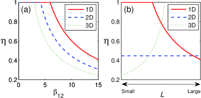
Figure 1: (Color online) (a) The overlap factor $\eta$ as a function of the reduced parameter $\beta_{12}$ [see Eq. (6)] in different dimensions (infinitely deep square well potential case, $g_{11}=g_{22}=0$). Note that for all values of $d$, there exists a critical value $\beta_{12}^{c}\neq 0$, below which $\eta$ attains its maximal possible value $1$. (b) a schematic plot of $\eta$ versus the width of the square well in different dimensions. Note the counter-intuitive fact that in the three dimensional case ($d=3$), the stronger we squeeze the system (the smaller $L$ is), the stronger phase separation is (the smaller $\eta$ is).

We have checked all these predictions numerically. Note that on the problem of phase separation, the intra-component interactions are on the same side as the kinetic energy—they both try to delocalize the condensates. Therefore, to highlight the effect of kinetic energy, we shall set $g_{11}=g_{22}=0$ ($\beta_{11}=\beta_{22}=0$), so that the kinetic energy is the only element acting against phase separation. As we shall see below, this special case also admits a simple analytical analysis.

We have solved the ground state of the system in all dimensions for a given value of $\beta_{12}$ bao . The overlap factor $\eta$ is plotted versus $\beta_{12}$ in Fig. 1a. We observe that in all dimensions, there exists a critical value of $\beta_{12}$ (denoted as $\beta_{12}^{c}$), below which the two condensates wave functions are equal ($\eta=1$). That is, for $\beta_{12}\leq\beta_{12}^{c}$, phase separation is completely suppressed. Above the critical value, phase separation develops ($\eta<1$) as $\beta_{12}$ increases, but is still greatly suppressed for a wide range of value of $\beta_{12}$. It should be stressed that though in Fig. 1a the curves of $\eta-\beta_{12}$ are qualitatively similar to each another for all values of $d$ (the plateau of $\eta=1$ is always located in the direction of $\beta_{12}\rightarrow 0$), the curves of $\eta-L$ will be quite different. The reason is that $\beta_{12}\propto L^{2-d}$. Figure 1b is a schematic plot of $\eta$ versus $L$ in all the three cases. It shows that $\eta$ as a function of $L$ is monotonically decreasing, constant, and monotonically increasing in one, two, and three dimensions, respectively. This means that to suppress phase separation, in one dimension we should tighten the confinement, in three dimensions we should loosen the confinement, while in two dimensions it is useless to change the confinement. Overall, Fig. 1 confirms the initial conjecture that kinetic energy can suppress phase separation.

As a hindsight, we can actually understand why phase separation can be suppressed in the limits of $L\rightarrow 0$ in one dimension and $L\rightarrow\infty$ in three dimensions. Consider two different configurations. The first one is a phase-separated one—the two condensates occupy the left and right halves of the container separately. The second one is a phase-mixed one—the two condensates both occupy the whole space available and thus overlap significantly. Compared with the first configuration, the second one costs more inter-component interaction energy which is on the order of $L^{-d}$, but saves more kinetic energy which is on the order of $L^{-2}$. The second configuration (phase-mixed) is more economical in energy in the limit of $L\rightarrow 0$ and $L\rightarrow\infty$, in the cases of $d=1$ and $d=3$, respectively. The case of $d=2$ is more subtle and which configuration wins depends on parameters other than $L$.

A remarkable fact revealed in Fig. 1 but not so obvious in our arguments is that in the symmetric case with $\beta_{11}=\beta_{22}=0$, $\eta=1$ for $\beta_{12}\leq\beta_{12}^{c}$, which is on the order of unity. This is a stronger fact than $\eta\rightarrow 1$ as $\beta_{12}\rightarrow 0$ as we argued. Actually, the general observation is that for $\beta_{11}=\beta_{22}>0$, $\eta=1$ for $\beta_{12}$ smaller than its critical value $\beta_{12}^{c}$, which is larger than $\beta_{11}$. This fact has rich meanings. On the one hand, it demonstrates that the kinetic energy is very effective—phase separation can be completely suppressed by it even if $\beta_{12}>\beta_{11}=\beta_{22}$, i.e., when (1) is satisfied. On the other hand, it strongly indicates that as $\beta_{12}$ crosses the critical value, the system undergoes a second order phase transition which can fit in the Landau formalism. The picture is that the exchange symmetry $\phi_{1}\leftrightarrow\phi_{2}$ of the energy functional (II) is preserved for $\beta_{12}<\beta_{12}^{c}$, but is spontaneously broken as $\beta_{12}$ surpasses $\beta_{12}^{c}$.

We have been able to prove the first point rigorously on the mathematical level (see Appendix A). However, it is also desirable to develop a physical understanding of the two points. This can be achieved by studying a two-component BEC in a double-well potential (see Appendix B) or using a variational approach pst6 . We note that in the limit of $\beta_{12}\rightarrow 0$, $\phi_{1,2}$ both converge to the (non-degenerate) ground state of a single particle in the $[-1/2,+1/2]^{d}$ infinitely deep square well. As $\beta_{12}$ is turned on, the two wave functions are deformed and excited states mix in. Because the energies of the excited states grow up quadratically, we cutoff at the first excited level and take the following ansatz for the two condensate wave functions

$$\phi_{1}=c_{0}\varphi_{0}+c_{1}\varphi_{1},\quad\phi_{2}=c_{0}\varphi_{0}-c_{1}\varphi_{1}.$$ (7)

Here $\varphi_{0}$ is the ground state, while $\varphi_{1}$ is one of the possibly degenerate first excited states. The coefficients $c_{0,1}$ are real and satisfy the normalization condition $c_{0}^{2}+c_{1}^{2}=1$. Obviously, complete phase mixing would correspond to $c_{1}=0$ while partial phase separation to $c_{1}\neq 0$. Our numerical simulations indicate that (this is also supported by the variational approach itself, see Appendix C) in the two dimensional case, when phase separation occurs, the two condensates are shifted either along $x$ or $y$ direction; in the three dimensional case, when phase separation occurs, the two condensates are shifted either along $x$ or $y$ or $z$ direction. This fact motivates us to choose $\varphi_{1}$ in the following form

$$d=1:\varphi_{1}=w_{1}(x);$$ (8a)

$$d=2:\varphi_{1}=w_{0}(x)w_{1}(y)\ \text{ or }\ w_{1}(x)w_{0}(y);$$ (8b)

$$d=3:\varphi_{1}=w_{0}(x)w_{0}(y)w_{1}(z)\ \text{ or }\ w_{0}(x)w_{1}(y)w_{0}(z)\quad$$

$$\quad\quad\quad\quad\quad\quad\text{ or }w_{1}(x)w_{0}(y)w_{0}(z),\quad\quad$$ (8c)

where $w_{0}(x)=\sqrt{2}\cos(\pi x)$ and $w_{1}(x)=\sqrt{2}\sin(2\pi x)$ are the ground and first excited states of a single particle in the one dimensional $[-1/2,+1/2]$ infinitely deep square well potential. Substituting Eqs. (7) and (8) into (II), we get the reduced energy functional $\widetilde{E}=E/(N\hbar^{2}/mL^{2})$ as

$$d=1:\widetilde{E}(c_{1})=(3\pi^{2}-5\beta_{12})c_{1}^{2}+5\beta_{12}c_{1}^{4}+\text{const};$$

$$d=2:\widetilde{E}(c_{1})=\left(3\pi^{2}-\frac{15}{2}\beta_{12}\right)c_{1}^{2}+\frac{15}{2}\beta_{12}c_{1}^{4}+\text{const};$$

$$d=3:\widetilde{E}(c_{1})=\left(3\pi^{2}-\frac{45}{4}\beta_{12}\right)c_{1}^{2}+\frac{45}{4}\beta_{12}c_{1}^{4}+\text{const}.$$

These are nothing but the Landau’s expression of the free energy in a second-order phase transition, with $c_{1}$ playing the role of the order parameter here. We immediately determine the critical values of $\beta_{12}$ by putting the coefficients of $c_{1}^{2}$ to zero. Specifically, $\beta_{12}^{c}=\frac{3\pi^{2}}{5}$, $\frac{2\pi^{2}}{5}$, and $\frac{4\pi^{2}}{15}$ for $d=1$, $d=2$, and $d=3$, respectively. These values agree with those extracted from Fig. 1 very well. The relative errors are within $1$%, $9$%, and $19$%, respectively. The deviation increases with $d$ because in higher dimensions, the degeneracy of the excited states increases and the two-mode approximation in (7) becomes less accurate. In the expressions of $\widetilde{E}$, we can actually see how the kinetic energy suppresses phase separation. The term $3\pi^{2}c_{1}^{2}$ comes from the kinetic energy difference of the two modes $\varphi_{1,2}$. Without this term, the critical value $\beta_{12}^{c}$ would be zero instead of being finite.

For a general case without the exchange symmetry $\phi_{1}\leftrightarrow\phi_{2}$, the appropriate order parameter is no longer $\eta$ but $\vec{r}_{m1}-\vec{r}_{m2}$. However, the second order transition picture still holds. Specifically, $\vec{r}_{m1}=0=\vec{r}_{m2}$ for $\beta_{12}$ smaller than some critical value $\beta_{12}^{c}$ which is larger than $\sqrt{\beta_{11}\beta_{22}}$. Overall, this asymmetric case is more involved than the symmetric case above because there are more parameters. Hopefully, a systematic study will be presented in a follow-up work.

III A two-component BEC in a harmonic potential

So far, we have focused on the ideal case of infinitely deep square wells. Experimentally, it is harmonic potentials that are most readily realized. Therefore, it is necessary to see whether analogous results hold for harmonic potentials. One concern is that the extra potential energy may blur the picture. However, after some similar rescaling, we shall see that all the results persist.

The energy functional of a two-component BEC in a $d$-dimensional isotropic harmonic potential is

$$\frac{E}{N}=\int_{R^{d}}d\vec{r}\bigg{\{}\frac{\hbar^{2}}{2m}\sum_{\alpha=1,2}|\nabla\psi_{\alpha}|^{2}+\frac{1}{2}m\omega_{d}^{2}|\vec{r}|^{2}\sum_{\alpha=1,2}|\psi_{\alpha}|^{2}$$

$$+\frac{N}{2}\left(g_{11}|\psi_{1}|^{4}+g_{22}|\psi_{2}|^{4}+2g_{12}|\psi_{1}|^{2}|\psi_{2}|^{2}\right)\bigg{\}}.\ \$$ (10)

Here again we have assumed equal mass and equal number for the two species. The two condensate wave functions are normalized to unity, i.e., $\int d\vec{r}|\psi_{1,2}|^{2}=1$. Now make the transform $\psi_{1,2}(\vec{r})=\xi_{ho}^{-d/2}\phi_{1,2}(\vec{x})$ with $\vec{r}=\xi_{ho}\vec{x}$, where $\xi_{ho}=\sqrt{\hbar/m\omega_{d}}$ is the characteristic length of the harmonic potential. We have then $\int d\vec{x}|\phi_{1,2}|^{2}=1$. In terms of $\phi_{1,2}$, the energy functional can be rewritten as

$$\frac{E}{N\hbar\omega_{d}}=\int_{R^{d}}d\vec{x}\bigg{\{}\frac{1}{2}\sum_{\alpha=1,2}|\nabla\phi_{\alpha}|^{2}+\frac{1}{2}|\vec{x}|^{2}\sum_{\alpha=1,2}|\phi_{\alpha}|^{2}\quad$$

$$+\frac{1}{2}\left(\beta_{11}|\phi_{1}|^{4}+\beta_{22}|\phi_{2}|^{4}+2\beta_{12}|\phi_{1}|^{2}|\phi_{2}|^{2}\right)\bigg{\}}.\quad$$ (11)

Here the reduced interaction strengths are defined as

$$\beta_{ij}=\frac{Nmg_{ij}\xi^{2-d}_{ho}}{\hbar^{2}}\propto\omega_{d}^{(d-2)/2},\ i,j=1,2.$$ (12)

We now have a similar situation as before. The importance of the interactions can be changed by changing the value of $\xi_{ho}$, which plays the role of $L$ in our previous example. The interactions will be negligible if $d=1$ and $\xi_{ho}\rightarrow 0$ or if $d=3$ and $\xi_{ho}\rightarrow\infty$. In this case, the rescaled wave functions $\phi_{1,2}$ will be close to the ground state of the harmonic oscillator, i.e., $\phi_{1,2}\simeq\pi^{-d/2}\exp(-\vec{x}^{2}/2)$, and phase separation is suppressed regardless of the values of the $g$’s. The interactions will become significant if $d=1$ and $\xi_{ho}\rightarrow\infty$ or $d=3$ and $\xi_{ho}\rightarrow 0$. In this case, the kinetic energy can be neglected and we enter the Thomas-Fermi regime. In this regime, the criterion (1) will be a faithful one for phase separation.

We have verified these predictions numerically. In Fig. 2, we have shown the overlap factor $\eta\equiv\int d\vec{x}\phi_{1}\phi_{2}$ versus the reduced inter-component interaction strength $\beta_{12}$ in all dimensions (with $g_{11}=g_{22}=g_{12}/1.05$). Again, we see that phase separation is completely suppressed for $\beta_{12}$ below some critical value $\beta_{12}^{c}$.

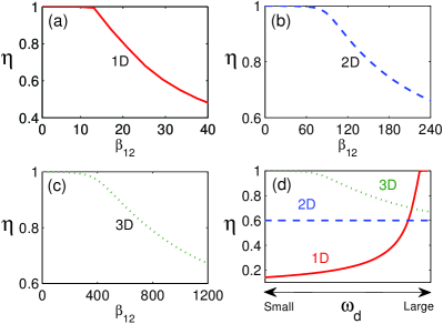
Figure 2: (Color online) (a)-(c) The overlap factor $\eta$ as a function of the reduced parameter $\beta_{12}$ [see Eq. (12)] in different dimensions (isotropic harmonic potential case, $g_{11}=g_{22}=g_{12}/1.05$). Note that for all value of $d$, there exists a critical value $\beta_{12}^{c}\neq 0$, below which $\eta$ attains its maximal possible value $1$. (d) a schematic plot of $\eta$ versus the characteristic frequency $\omega_{d}$ of the harmonic potential in different dimensions.

Let us now consider the possibility of experimentally observing the immiscibility-miscibility transition by adjusting the confinement, e.g., the frequency $\omega_{d}$. In cold atom experiments, the harmonic potential is often of the form $V(\vec{r})=\frac{1}{2}m[\omega_{\perp}^{2}(x^{2}+y^{2})+\omega_{z}^{2}z^{2}]$. To get a three dimensional isotropic potential, we set $\omega_{\perp}=\omega_{z}$. An effectively one (two) dimensional potential can be obtained in the limit of $\omega_{\perp}\gg\omega_{z}$ ($\omega_{\perp}\ll\omega_{z}$). For these three different geometries of the potential, the interaction strengths (the $g$’s) relate to the $s$-wave scattering lengths (the $a$’s) as

$$g_{ij}\! = \frac{4\pi\hbar a_{ij}}{m},\ \omega_{d}=\omega_{z}=\omega_{\perp},\ d=3;$$ (13a)

$$g_{ij}\! = \frac{2\sqrt{2\pi}\hbar^{3/2}\omega_{z}^{1/2}a_{ij}}{m^{1/2}},\ \omega_{d}=\omega_{\perp}\!\ll\omega_{z},\ d=\!2;\quad$$ (13b)

$$g_{ij}\! = 2\hbar a_{ij}\omega_{\perp},\ \omega_{d}=\omega_{z}\ll\omega_{\perp},\ d=1.$$ (13c)

Using Eqs. (12) and (13), we can study the possibility of tuning $\beta_{12}$ across the critical value $\beta_{12}^{c}$. We study each case individually (the mass $m$ is taken to be that of ²³Na):

(i) $d=3$. Suppose $N=10^{4}$, $a_{12}=40$ $a_{\text{B}}$. The critical value of $\omega_{d}$ is $2\pi\times 560$ Hz, which can be covered in current experiments.

(ii) $d=2$. Suppose $N=10^{4}$, $a_{12}=40$ $a_{\text{B}}$, and the transverse frequency $\omega_{\perp}=2\pi\times 2.6$ Hz. The critical value of the longitudinal frequency $\omega_{z}$ is $2\pi\times 140$ Hz, which is realizable in current experiments papp08 .

(iii) $d=1$. Suppose $N=2\times 10^{3}$, $a_{12}=40$ $a_{\text{B}}$, and the transverse frequency $\omega_{\perp}=2\pi\times 130$ Hz. The critical value of the longitudinal frequency $\omega_{z}$ is $2\pi\times 19$ Hz, which is realizable in current experiments.

Here the number of atoms is one or two orders smaller than its typical value in experiments. This explains why the criterion (1) is a reliable one in the experiments in papp08 ; thalhammer08 . They work in a regime where the kinetic energy is indeed negligible. However, with the advance of imaging techniques, hopefully future experiments can work with a relatively small number of atoms and observe the miscibility-immiscibility transition by changing the confinement.

IV Conclusions

To conclude, we have demonstrated that kinetic energy can play a vital role in determining the configuration of a two-component BEC. It renders the empirical condition of phase separation $g_{11}g_{22}<g_{12}^{2}$ insufficient and it also modifies the picture of phase separation. To be specific, phase separation can be completely suppressed even if this condition is fulfilled. Moreover, the phase mixing to phase separation transition is now known to be a second-order, continuous transition instead of a first-order, discontinuous one as in the usual view. From the experimental point of view, our results may provide a new scenario of controlling the transition of phase mixing-demixing of a two-component BEC. Instead of adjusting the interaction strengths, one can just change the confinement, the characteristic size of the container.

V Acknowledgments

We are grateful to Weizhu Bao, L. You, and C. H. Lee for helpful discussions. This work is supported by NSF of China under Grant No. 11091240226, the Ministry of Science and Technology of China 973 program (2012CV821400) and NSFC-1190024. Y. Cai acknowledges support from the Academic Research Fund of Ministry of Education of Singapore grant R-146-000-120-112.

Appendix A Rigorous justification

Here, we consider the energy functional as

$$E[\phi_{1},\phi_{2}]=\int_{\Omega_{0}}d\vec{x}\bigg{\{}\frac{1}{2}|\nabla\phi_{1}|^{2}+\frac{1}{2}|\nabla\phi_{2}|^{2}\qquad\qquad\qquad$$ (14)

$$+\frac{1}{2}\left(\beta_{11}|\phi_{1}|^{4}+\beta_{22}|\phi_{2}|^{4}+2\beta_{12}|\phi_{1}|^{2}|\phi_{2}|^{2}\right)\bigg{\}},$$

where $\Omega_{0}=[-\frac{1}{2},\frac{1}{2}]^{d}$ ($d=1,2,3$), $\beta_{11}=\beta_{22}=\beta$. Let $\phi_{g}$ be the unique positive ground state of the energy functional $E_{s}[\phi]\equiv E[\phi,\phi]$, and $\mu_{g}$ be the corresponding chemical potential. The functions $\phi_{1,2}$ are normalized to unity by the usual $L^{2}$-norm. Let $(\phi^{g}_{1},\phi_{2}^{g})$ be the positive ground state of (14). For $\beta_{12}\leq\beta$, $E[\sqrt{\rho_{1}},\sqrt{\rho_{2}}]$ ($\rho_{1}\equiv|\phi_{1}|^{2}$, $\rho_{2}\equiv|\phi_{2}|^{2}$) is strictly convex in $(\rho_{1},\rho_{2})$ Lie ; 2bec , and the positive ground state is unique, i.e., $\phi_{1}^{g}=\phi_{2}^{g}=\phi_{g}$, $\eta=1$. We are going to prove that there exists a critical value $\beta_{12}^{c}>\beta$ such that when $\beta_{12}<\beta_{12}^{c}$, there holds $\phi_{1}^{g}=\phi_{2}^{g}=\phi_{g}$, i.e., $\eta=1$. From now on, we concentrate on the case of $\beta_{12}\geq\beta$ and assume that $\beta_{12}=\beta+\beta^{\prime}$, $0\leq\beta^{\prime}\leq 1$. Simple calculation shows that

$$E[\phi_{1}^{g},\phi_{2}^{g}]-E[\phi_{g},\phi_{g}]=\int_{\Omega_{0}}d\vec{x}\sum\limits_{\alpha=1,2}\bigg{\{}\frac{1}{2}|\nabla(\phi_{\alpha}^{g}-\phi_{g})|^{2}$$

$$+(\beta+\beta_{12})|\phi_{g}|^{2}|\phi_{\alpha}^{g}-\phi_{g}|^{2}+\frac{\beta-\beta_{12}}{2}\left(|\phi_{\alpha}^{g}|^{2}-|\phi_{g}|^{2}\right)^{2}$$

$$+\nabla(\phi_{\alpha}^{g}-\phi_{g})\cdot\nabla\phi_{g}+2(\beta+\beta_{12})|\phi_{g}|^{2}\phi_{g}(\phi_{\alpha}^{g}-\phi_{g})\bigg{\}}$$

$$+\frac{\beta_{12}}{2}\left(|\phi_{1}^{g}|^{2}+|\phi_{2}^{g}|^{2}-2|\phi_{g}|^{2}\right)^{2}.$$

Making use of the Euler-Lagrange equation of $\phi_{g}$,

$$\mu_{g}\phi_{g}=-\frac{1}{2}\nabla^{2}\phi_{g}+(\beta+\beta_{12})|\phi_{g}|^{2}\phi_{g},$$ (15)

denoting $e_{\alpha}=\phi_{\alpha}^{g}-\phi_{g}$ ($\alpha=1,2$), and noticing $\int_{\Omega_{0}}e_{\alpha}\phi_{g}=-\frac{1}{2}\|e_{\alpha}\|_{2}^{2}$, we obtain

$$E[\phi_{1}^{g},\phi_{2}^{g}]-E[\phi_{g},\phi_{g}]=\int_{\Omega_{0}}d\vec{x}\sum\limits_{\alpha=1,2}\bigg{\{}\frac{1}{2}|\nabla e_{\alpha}|^{2}$$

$$+(\beta+\beta_{12})|\phi_{g}|^{2}|e_{\alpha}|^{2}-\frac{\beta^{\prime}}{2}\left(|\phi_{\alpha}^{g}|^{2}-|\phi_{g}|^{2}\right)^{2}$$

$$+2\mu_{g}\phi_{g}e_{\alpha}\bigg{\}}+\frac{\beta_{12}}{2}\left(|\phi_{1}^{g}|^{2}+|\phi_{2}^{g}|^{2}-2|\phi_{g}|^{2}\right)^{2}.$$

Now, the operator $L_{g}=-\frac{1}{2}\nabla^{2}+(\beta+\beta_{12})|\phi_{g}|^{2}$ admits eigenvalues as $\mu_{g}<\mu_{1}\leq\mu_{2}\leq\cdots$, and the eigenfunction $\phi_{g}$ corresponds to $\mu_{g}$, $w_{k}\in H_{0}^{1}$ with $\|w_{k}\|_{2}=1$ corresponds to $\mu_{k}$ ($k\geq 1$). The reason $\phi_{g}$ is the ground state comes from the positivity of $\phi_{g}$ and the uniqueness of the positive ground state of $L_{g}$. Expand $e_{\alpha}$ as $e_{\alpha}=c_{g}^{\alpha}\phi_{g}+\sum_{k=1}^{\infty}c^{\alpha}_{k}w_{k}$, then $(c_{g}^{\alpha})^{2}+\sum_{k=1}^{\infty}|c^{\alpha}_{k}|^{2}=\|e_{\alpha}\|_{2}^{2}$, $c_{g}^{\alpha}=\int_{\Omega_{0}}e_{\alpha}\phi_{g}=-\frac{1}{2}\|e_{\alpha}\|_{2}^{2}$ and we can derive that

$$\int_{\Omega_{0}}d\vec{x}\bigg{\{}\frac{1}{2}|\nabla e_{\alpha}|^{2}+(\beta+\beta_{12})|\phi_{g}|^{2}|e_{\alpha}|^{2}+2\mu_{g}\phi_{g}e_{\alpha}\bigg{\}}$$

$$=\mu_{g}(c_{g}^{\alpha})^{2}+\sum\limits_{k=1}^{\infty}\mu_{k}|c^{\alpha}_{k}|^{2}-\mu_{g}\|e_{\alpha}\|_{2}^{2}$$

$$\geq(\mu_{1}-\mu_{g})(\|e_{\alpha}\|_{2}^{2}-(c_{g}^{\alpha})^{2})$$

$$=(\mu_{1}-\mu_{g})\|e_{\alpha}\|_{2}^{2}(1-\|e_{g}^{\alpha}\|_{2}^{2}/4).$$

Now, firstly, we need a lower bound for $\mu_{1}-\mu_{g}$, the so-called fundamental gap, which has been solved recently by A. Ben and C. Julie fund . Using equation (15), applying elliptic theory with convex domain $\Omega_{0}$, it is easy to verify that $\phi_{g}\in H^{2}(\Omega_{0})$ and hence belongs to $C^{0,\gamma}(\overline{\Omega_{0}})$ ($0<\gamma<\frac{1}{2}$) by Sobolev embedding. Approximating $\Omega_{0}$ by convex domain $\Omega_{\varepsilon}$ (with smooth boundary) and applying Schauder estimates, we shall have $\phi_{g}\in C^{2,\gamma}(\overline{\Omega_{\varepsilon}})$ and there exists some $c>0$ such that $|\phi_{g}|^{2}+c|\vec{x}|^{2}$ is convex (as Hessian matrix of $|\phi_{g}|^{2}$ is bounded by Schauder estimates). Hence, we can apply the results in Ref. fund to get ($D_{\varepsilon}$ is the diameter of $\Omega_{\varepsilon}$)

$$\mu_{1}^{\varepsilon}-\mu_{g}^{\varepsilon}\geq\frac{3\pi^{2}}{D_{\varepsilon}^{2}},$$ (16)

where $\mu_{g}^{\varepsilon}$ and $\mu_{1}^{\varepsilon}$ are the first and second eigenvalues, respectively, of $L_{g}$ in $H_{0}^{1}(\Omega_{\varepsilon})$. By Min-max principles, letting $\varepsilon\to 0$, we have $\mu_{g}^{\varepsilon}\to\mu_{g}$ and $\mu_{1}^{\varepsilon}\to\mu_{1}$. Hence we find

$$\mu_{1}-\mu_{g}\geq\frac{3\pi^{2}}{D^{2}},$$ (17)

where $D$ is the diameter of $\Omega_{0}$ [or if we assume $\Omega_{0}$ is a convex domain with smooth boundaries, (17) follows directly].

Secondly, we have $\|e_{\alpha}\|_{2}^{2}\leq\int_{\Omega_{0}}d\vec{x}(|\phi_{\alpha}^{g}|^{2}+|\phi_{g}|^{2})=2$.

Thirdly, we would like to derive $L^{\infty}$ bounds of $\phi_{g}$ and $\phi_{\alpha}^{g}$. The Euler-Lagrange equation for $\phi_{\alpha}^{g}$ reads as

$$\mu_{\alpha}^{g}\phi_{\alpha}^{g}=-\frac{1}{2}\nabla^{2}\phi_{\alpha}^{g}+\beta|\phi_{\alpha}^{g}|^{2}\phi_{\alpha}^{g}+\beta_{12}|\phi_{\alpha^{\prime}}^{g}|^{2}\phi_{\alpha}^{g},$$ (18)

with $\alpha^{\prime}\neq\alpha$. For the nonlinear eigenvalues, we have the estimates $\mu_{\alpha}^{g}\leq 2E[\phi_{1}^{g},\phi_{2}^{g}]\leq 2E_{s}[\phi_{g}]$, $\mu_{g}\leq E_{s}[\phi_{g}]$ and $E_{s}[\phi_{g}]$ can be bounded by choosing any test function (like the ground state of $-\Delta$), which gives $E_{s}[\phi_{g}]\leq\widetilde{C}(1+\beta)$ ($\widetilde{C}$ depends on $\Omega_{0}$).

If $\beta\geq 1$, considering the point $x_{0}\in\Omega_{0}$ where $\phi_{g}$ attains its maximum, then $\Delta\phi_{g}(x_{0})\leq 0$ and from (15), we have

$$\mu_{g}\phi_{g}(x_{0})\geq(\beta+\beta_{12})|\phi_{g}(x_{0})|^{2}\phi_{g}(x_{0}),$$

which gives $\|\phi_{g}\|_{\infty}^{2}\leq\frac{\mu_{g}}{\beta+\beta_{12}}\leq 2\widetilde{C}$. Similarly, we can obtain the $L^{\infty}$ bound for $\phi_{\alpha}^{g}$ using the Euler-Lagrange equation and $\|\phi_{\alpha}^{g}\|_{\infty}^{2}\leq\frac{\mu_{\alpha}^{g}}{\beta}\leq 4\widetilde{C}$. Thus, $\|\phi_{g}+\phi_{\alpha}^{g}\|_{\infty}^{2}\leq 12\widetilde{C}$. Combining the three observations above, we get

$$E[\phi_{1}^{g},\phi_{2}^{g}]-E[\phi_{g},\phi_{g}]\geq\sum\limits_{\alpha=1,2}\bigg{\{}\frac{3\pi^{2}}{2D^{2}}-\frac{12\beta^{\prime}\widetilde{C}}{2}\bigg{\}}\|e_{\alpha}\|_{2}^{2},$$

which implies that for $0\leq\beta^{\prime}\leq\min\{\frac{\pi^{2}}{4D^{2}\widetilde{C}},1\}$, there must hold $e_{\alpha}=0$, i.e., $\eta=1$.

For $\beta\in[0,1]$, the approach above is not good. In this case, we see that $\mu_{\alpha}^{g}\leq 4\widetilde{C}$ and $\mu_{g}\leq 2\widetilde{C}$. Using Sobolev inequality, in one dimension ($d=1$), we can find that

$$\|\phi_{\alpha}^{g}\|_{\infty}^{2}\leq\|\nabla\phi_{\alpha}^{g}\|_{2}\|\phi_{\alpha}^{g}\|_{2}\leq\sqrt{\mu_{\alpha}^{g}}\leq 2\sqrt{\widetilde{C}}.$$ (19)

Similarly, $\|\phi_{g}\|_{\infty}^{2}\leq\sqrt{2\widetilde{C}}$. For two and three dimensions ($d=2,3$), recalling (15) and (18), we can obtain from elliptic theory and Sobolev inequalities that there exist constants $C_{1},C_{2}>0$ only depending on $\Omega_{0}$ such that $\|\phi_{\alpha}^{g}\|_{\infty}\leq C_{1}\|\phi_{\alpha}^{g}\|_{H^{2}}\leq C_{2}\cdot\|\mu_{\alpha}^{g}\phi_{\alpha}^{g}-\beta|\phi_{\alpha}^{g}|^{2}\phi_{\alpha}^{g}-\beta_{12}|\phi_{\alpha^{\prime}}^{g}|^{2}\phi_{\alpha}^{g}\|_{2}$, and $\|\phi_{g}\|_{\infty}\leq C_{2}\|\mu_{g}\phi_{g}-(\beta+\beta_{12})|\phi_{g}|^{2}\phi_{g}\|_{2}$. In two and three dimensions, using Sobolev inequality, we have $\|\phi_{\alpha}^{g}\|_{6}\leq C_{3}\|\nabla\phi_{\alpha}^{g}\|_{2}\leq C_{3}\sqrt{\mu_{\alpha}^{g}}$ ($C_{3}$ depends on $\Omega_{0}$). Cauchy inequality leads to

$$\|\phi_{\alpha}^{g}\|_{\infty}\leq C_{2}(\mu_{\alpha}^{g}+\beta\|\phi_{\alpha}^{g}\|_{6}^{3}+\beta_{12}\|\phi_{\alpha}^{g}\|_{6}\|\phi_{\alpha^{\prime}}^{g}\|_{6}^{2}),$$

and thus $\|\phi_{\alpha}^{g}\|_{\infty}^{2}\leq C_{4}$ ($C_{4}$ depends on $\Omega_{0}$). Similarly, $\|\phi_{g}\|_{\infty}^{2}\leq C_{5}$ ($C_{5}$ depends on $\Omega_{0}$). Eventually, we have in all dimensions ($d=1,2,3$), there exists a constant $C_{\Omega_{0}}$ depending only on $\Omega_{0}$ such that $\|\phi_{\alpha}^{g}+\phi_{g}\|_{\infty}^{2}\leq C_{\Omega_{0}}$. Similar to the case with $\beta\geq 1$, we have

$$E[\phi_{1}^{g},\phi_{2}^{g}]-E[\phi_{g},\phi_{g}]\geq\sum\limits_{\alpha=1,2}\left\{\frac{3\pi^{2}}{2D^{2}}-\frac{\beta^{\prime}C_{\Omega_{0}}}{2}\right\}\|e_{\alpha}\|_{2}^{2},$$

which leads to the conclusion that when $\beta^{\prime}<\min\{1,\frac{3\pi^{2}}{D^{2}C_{\Omega_{0}}}\}$, $\phi_{\alpha}^{g}=\phi_{g}$, i.e., $\eta=1$. In summary, for all $\beta\geq 0$, if we choose $\beta_{12}^{c}=\beta+\min\{1,\frac{3\pi^{2}}{D^{2}C_{\Omega_{0}}},\frac{\pi^{2}}{4D^{2}\widetilde{C}}\}>\beta$, then for all $0\leq\beta_{12}<\beta_{12}^{c}$, we shall have $\eta=1$.

Appendix B Phase separation as a spontaneous symmetry breaking

Consider a two-component BEC in a symmetric double-well potential. Under the two-mode approximation, the mean-field energy functional is

$$E = -J_{a}(\psi_{a1}^{*}\psi_{a2}+\psi_{a2}^{*}\psi_{a1})-J_{b}(\psi_{b1}^{*}\psi_{b2}+\psi_{b2}^{*}\psi_{b1})$$ (20)

$$+\frac{1}{2}U_{a}(|\psi_{a1}|^{4}+|\psi_{a2}|^{4})+\frac{1}{2}U_{b}(|\psi_{b1}|^{4}+|\psi_{b2}|^{4})$$

$$+V(|\psi_{a1}|^{2}|\psi_{b1}|^{2}+|\psi_{a2}|^{2}|\psi_{b2}|^{2}).$$

Here $J_{a}$ and $J_{b}$ are the hopping amplitudes of the two types of atoms, and $U_{a}$ and $U_{b}$ are the intra-component onsite interaction strengths, while $V$ is the inter-component one. The complex numbers $\psi_{a1}$ and $\psi_{b1}$ ($\psi_{a2}$ and $\psi_{b2}$) are the amplitudes of the two condensate wave functions on the left (right) trap. They are constrained by the total atom numbers, i.e., $|\psi_{a1}|^{2}+|\psi_{a2}|^{2}=N_{a}$ and $|\psi_{b1}|^{2}+|\psi_{b2}|^{2}=N_{b}$. For the sake of simplicity, in the following we shall assume $J_{a}=J_{b}=J\geq 0$, $U_{a}=U_{b}=U\geq 0$, and $N_{a}=N_{b}=N$. As far as the ground state is concerned, it is legitimate to assume the $\psi$’s real and positive. Therefore, we can write $\psi_{a1}=\sqrt{N_{a1}}$, $\psi_{b1}=\sqrt{N_{b1}}$ and similarly for other $\psi$’s.

First assume tunneling is turned off, i.e. $J=0$. Let $N_{a1}=\frac{1}{2}N+\delta_{a}$ and $N_{b1}=\frac{1}{2}N-\delta_{b}$. The energy (20) is

$$E(\delta_{a},\delta_{b})=U(\delta_{a}^{2}+\delta_{b}^{2})-2V\delta_{a}\delta_{b}+\text{const}.$$ (21)

It is readily determined that if $U>V$, the ground state is of $\delta_{a}=\delta_{b}=0$. The two condensates are both distributed evenly between the two wells, which is a completely mixed configuration. If $U<V$ [the counterpart of (1) in the present context], the ground state is of $(\delta_{a},\delta_{b})=\pm(N/2,N/2)$, which corresponds to complete phase separation—the two condensates occupy the two wells separately. Therefore, without tunneling, the miscibility-immiscibility transition is a first-order phase transition with the critical point being $V^{c}=U$.

Now turn on the tunneling. For the sake of simplicity, suppose $\delta_{a}=\delta_{b}=\delta$. The energy as a function of the order parameter $\delta$ is

$$E = -4J\sqrt{\left(\frac{N}{2}\right)^{2}-\delta^{2}}+2(U-V)\delta^{2}+\text{const}$$ (22)

$$= \left[\frac{4J}{N}+2(U-V)\right]\delta^{2}+\frac{4J}{N^{3}}\delta^{4}+o(\delta^{4})+\text{const}.\quad\quad$$

Here we have the familiar Landau formalism for second order phase transitions. The coefficient of the quartic term is positive but the sign of the quadratic term changes from positive to negative as $V$ surpasses the critical value $V^{c}=U+2J/N$. Corresponding, $\delta=0$ is turned from a minimum to a maximum point and phase separation develops. Here we note that the tunneling, the kinetic term in the present context, has two consequences. First, the first-order transition is turned into a second-order one. Second, the transition point is up shifted from $U$ to $U+2J/N$. This is reasonable since phase separation costs kinetic energy. What presented in Figs. 1 and 2 are parallel to these results but in continuum (multi-mode) cases.

Appendix C Justification of the form of $\varphi_{1}$ in Eq. (8)

In this Appendix, we show why among all the (degenerate) first excited states, the one in Eq. (8) is selected. For $d=2$, the ansatz more general than Eq. (7) is

$$\phi_{1} = c_{0}\varphi_{0}+c_{x}\varphi_{x}+c_{y}\varphi_{y},$$ (23a)

$$\phi_{2} = c_{0}\varphi_{0}-c_{x}\varphi_{x}-c_{y}\varphi_{y},$$ (23b)

with $\varphi_{x}=w_{1}(x)w_{0}(y)$, $\varphi_{y}=w_{0}(x)w_{1}(y)$, and $c_{0}$, $c_{x}$, $c_{y}$ being some real variables under the constraint $c_{0}^{2}+c_{x}^{2}+c_{y}^{2}=1$. Substituting Eq. (23) into Eq. (II), we get the reduced energy functional $\widetilde{E}=E/(N\hbar^{2}/mL^{2})$ as a function of $c_{x,y}$ as

$$\tilde{E}[c_{x},c_{y}] = 2\pi^{2}+\frac{9}{4}\beta_{12}+\left(3\pi^{2}-\frac{15}{2}\beta_{12}\right)(c_{x}^{2}+c_{y}^{2})$$ (24)

$$+\frac{15}{2}\beta_{12}\left(c_{x}^{2}+c_{y}^{2}\right)^{2}+\frac{3}{2}\beta_{12}c_{x}^{2}c_{y}^{2}.$$

We see that for $\beta\leq\beta_{12}^{c}=\frac{2}{5}\pi^{2}$, the minimum is at $c_{x}=c_{y}=0$. For $\beta_{12}>\beta_{12}^{c}$, the minimum is no longer at the origin. However, for a fixed value of $c_{x}^{2}+c_{y}^{2}$, $\tilde{E}$ is minimized when the last term in Eq. (24) vanishes or when $c_{x}=0$ or $c_{y}=0$. That is why the particular ansatz in Eqs. (7) and (8) is appropriate and enough. We note that due to the symmetry of the trap, the reduced energy functional is invariant under the transform $(c_{x},c_{y})\rightarrow(\pm c_{x},\pm c_{y})$ and $(c_{x},c_{y})\rightarrow(c_{y},c_{x})$. This symmetry is broken when phase separation occurs.

Similar analysis applies for $d=3$. In this case, the ansatz more general than Eq. (7) is

$$\phi_{1} = c_{0}\varphi_{0}+c_{x}\varphi_{x}+c_{y}\varphi_{y}+c_{z}\varphi_{z},$$ (25a)

$$\phi_{2} = c_{0}\varphi_{0}-c_{x}\varphi_{x}-c_{y}\varphi_{y}-c_{z}\varphi_{z},$$ (25b)

with $\varphi_{x}=w_{1}(x)w_{0}(y)w_{0}(z)$, $\varphi_{y}=w_{0}(x)w_{1}(y)w_{0}(z)$, $\varphi_{z}=w_{0}(x)w_{0}(y)w_{1}(z)$, and $c_{0}$, $c_{x}$, $c_{y}$, $c_{z}$ being some real variables under the constraint $c_{0}^{2}+c_{x}^{2}+c_{y}^{2}+c_{z}^{2}=1$. Substituting Eq. (25) into Eq. (II), we get the reduced energy functional $\tilde{E}$ as a function of $c_{x,y,z}$ as

$$\tilde{E} = 3\pi^{2}+\frac{27}{8}\beta_{12}+\left(3\pi^{2}-\frac{45}{4}\beta_{12}\right)(c_{x}^{2}+c_{y}^{2}+c_{z}^{2})\quad\quad\$$ (26)

$$\quad\quad+\frac{45}{4}\beta_{12}\left(c_{x}^{2}+c_{y}^{2}+c_{z}^{2}\right)^{2}$$

$$\quad\quad+\frac{9}{4}\beta_{12}\left(c_{x}^{2}c_{y}^{2}+c_{y}^{2}c_{z}^{2}+c_{z}^{2}c_{x}^{2}\right).$$

We see that for $\beta\leq\beta_{12}^{c}=\frac{4}{15}\pi^{2}$, the minimum is at $c_{x}=c_{y}=c_{z}=0$. For $\beta_{12}>\beta_{12}^{c}$, the minimum is no longer at the origin. However, for a fixed value of $c_{x}^{2}+c_{y}^{2}+c_{z}^{2}$, $\tilde{E}$ is minimized when the last term in Eq. (26) vanishes or when two of the three $c$’s are zero. Again, we see that the particular ansatz in Eqs. (7) and (8) is appropriate and enough.

References

• (1) P. K. Khabibullaev and A. A. Saidov, Phase Separation in Soft Matter Physics (Springer, Berlin, 2003).
• (2) E. Dagotto, Nanoscale Phase Separation and Colossal Magneto-resistance (Springer, Berlin, 2003).
• (3) K. Huang, Statistical Mechanics (John Wiley & Sons, New York, 1963).
• (4) C. J. Myatt, E. A. Burt, R. W. Ghrist, E. A. Cornell, and C. E. Wieman, Phys. Rev. Lett. 78, 586 (1997).
• (5) D. M. Stamper-Kurn, M. R. Andrews, A. P. Chikkatur, S. Inouye, H.-J. Miesner, J. Stenger, and W. Ketterle, Phys. Rev. Lett. 80, 2027 (1998).
• (6) D. S. Hall, M. R. Matthews, J R. Ensher, C. E. Wieman, and E. A. Cornell, Phys. Rev. Lett. 81, 1539 (1998).
• (7) G. Modugno, G. Ferrari, G. Roati, R. J. Brecha, A. Simoni, and M. Inguscio, Science 294, 1320 (2001).
• (8) M. Mudrich, S. Kraft, K. Singer, R. Grimm, A. Mosk, and M. Weidemüller, Phys. Rev. Lett. 88, 253001 (2002).
• (9) C. J. Pethick and H. Smith, Bose-Einstein Condensation in Dilute Gases (Cambridge University Press, Cambridge, England, 2002).
• (10) L. Pitaevskii, S. Stringari, Bose-Einstein Condensation (Oxford University Press, New York, 2003).
• (11) To avoid the possibility of collapse of the BEC under attractive interaction, throughout this paper all the $g$’s are assumed to be non-negative.
• (12) S. B. Papp, J. M. Pino, and C. E. Wieman, Phys. Rev. Lett. 101, 040402 (2008).
• (13) G. Thalhammer, G. Barontini, L. D. Sarlo, J. Catani, F. Minardi, and M. Inguscio, Phys. Rev. Lett. 100, 210402 (2008).
• (14) I. M. Merhasin, B. A. Malomed, and R. Driben, J. Phys. B 38, 877 (2005).
• (15) Note that the scenario here is like that in malomed , where the Rabi coupling between the two components favors phase mixing and thus can suppress phase separation.
• (16) W. Bao and Q. Du, SIAM J. Sci. Comput. 25, 1674 (2004).
• (17) R. Navarro, R. Carretero-González, and P. G. Kevrekidis, Phys. Rev. A 80, 023613 (2009).
• (18) E. H. Lieb, R. Seiringer, and J. Yngvason, Phy. Rev. A 61, 043602 (2000).
• (19) W. Bao and Y. Cai, East Asia Journal on Applied Mathematics 1, 49 (2011).
• (20) A. Ben and C. Julie, J. Amer. Math. Soc. 24, 899 (2011).