The Horizontal Component of Photospheric Plasma Flows During the Emergence of Active Regions on the Sun

Abstract

The dynamics of horizontal plasma flows during the first hours of the emergence of active region magnetic flux in the solar photosphere have been analyzed using SOHO/MDI data. Four active regions emerging near the solar limb have been considered. It has been found that extended regions of Doppler velocities with different signs are formed in the first hours of the magnetic flux emergence in the horizontal velocity field. The flows observed are directly connected with the emerging magnetic flux; they form at the beginning of the emergence of active regions and are present for a few hours. The Doppler velocities of flows observed increase gradually and reach their peak values 4 – 12 hours after the start of the magnetic flux emergence. The peak values of the mean (inside the $\pm$500  $\mathrm{m\,s^{-1}}$ isolines) and maximum Doppler velocities are 800 – 970  $\mathrm{m\,s^{-1}}$ and 1410 – 1700  $\mathrm{m\,s^{-1}}$, respectively. The Doppler velocities observed substantially exceed the separation velocities of the photospheric magnetic flux outer boundaries. The asymmetry was detected between velocity structures of leading and following polarities. Doppler velocity structures located in a region of leading magnetic polarity are more powerful and exist longer than those in regions of following polarity. The Doppler velocity asymmetry between the velocity structures of opposite sign reaches its peak values soon after the emergence begins and then gradually drops within 7 – 12 hours. The peak values of asymmetry for the mean and maximal Doppler velocities reach 240 – 460  $\mathrm{m\,s^{-1}}$ and 710 – 940  $\mathrm{m\,s^{-1}}$, respectively. An interpretation of the observable flow of photospheric plasma is given.

1 Introduction

sec:intro

According to measurements of Doppler velocities during the emergence of active regions in the solar photosphere, the presence of upflows at the tops [Brants (1985a), Brants (1985b), Tarbell et al. (1989), Lites, Skumanich, and Martinez Pillet (1998), Strous and Zwaan (1999), Kubo, Shimizu, and Lites (2003), Guglielmino et al. (2006), Grigor’ev, Ermakova, and Khlystova (2007), Grigor’ev, Ermakova, and Khlystova (2009)] and downflows of plasma at the footpoints [Gopasyuk (1967), Gopasyuk (1969), Kawaguchi and Kitai (1976), Bachmann (1978), Zwaan, Brants, and Cram (1985), Brants (1985a), Brants (1985b), Brants and Steenbeek (1985), Lites, Skumanich, and Martinez Pillet (1998), Solanki et al. (2003), Lagg et al. (2007), Xu, Lagg, and Solanki (2010)] of the emerging magnetic loops is well-established.

Uptil now horizontal photospheric velocities accompanying the emergence of active regions have only been measured indirectly. fra72 studied a young active region and found that the photospheric magnetic field knots (21 events) moved along the arch filament system (AFS) at velocities of 0.1 – 0.4  $\mathrm{km\,s^{-1}}$. Using observations of the young active region for 6.5 hours, sch73 found that magnetic elements moved in random directions with velocities of 0.4 – 1.0  $\mathrm{km\,s^{-1}}$. bar90 measured the separation velocities of the opposite polarities for 45 bipolar pairs in the young active region and obtained velocity values up to 0.5 – 3.5  $\mathrm{km\,s^{-1}}$, decreasing with time. str99 considered the emerging magnetic flux in a growing active region and found that the footpoints of the magnetic loops separated at an average velocity of 1.4  $\mathrm{km\,s^{-1}}$. gri09 estimated the separation velocities of the photospheric magnetic flux outer boundaries in the NOAA 10488 active region. The velocities decreased as the magnetic flux emerged: they were 2 – 2.5  $\mathrm{km\,s^{-1}}$ at the end of the first hour and 0.3  $\mathrm{km\,s^{-1}}$ in two and a half hours.

High values of horizontal photospheric velocities were obtained during the emergence of ephemeral active regions, except for the work of cho87. har73 found that during the first 30 minutes of the emergence of ephemeral active regions the footpoints of magnetic loops separated at 5  $\mathrm{km\,s^{-1}}$; the divergence velocity decreased to 0.7 – 1.3  $\mathrm{km\,s^{-1}}$ over the next six hours and continued to decrease later on. cho87 obtained low separation velocities of opposite polarities of 0.2 – 1  $\mathrm{km\,s^{-1}}$ for 24 emerging ephemeral active regions. hag01 found that the outer boundaries of the ephemeral regions expand with velocities up to 5.5  $\mathrm{km\,s^{-1}}$; there is a tendency for the velocities to decrease with time.

ots11 studied 101 emerging flux regions of different spatial scales. They found that the separation velocities of opposite polarities are lower than 1  $\mathrm{km\,s^{-1}}$ for large emerging magnetic fluxes, whereas they reach 4  $\mathrm{km\,s^{-1}}$ in small-scale ones.

Interesting results were obtained from the analysis of horizontal flows in the emerging active regions by granular motion. str96 found large-scale horizontal divergent granular flows in a growing active region which were comparable with the common drift of magnetic polarities. The authors interpreted this fact as a close interaction between granulation and magnetic fields. koz05 and koz06 also found divergent flows located between the footpoints of emerging flux loops. These authors consider these flows to be either convective flows which may trigger magnetic flux emergence from deep layers. They also suggest that the observed flows are formed by the emergence of magnetic flux. Note that the articles listed above concerned developing active regions already containing pores.

The present investigation involves an analysis of photospheric Doppler velocities for active regions emerging near the limb. This subject was considered earlier by khl11.

2 Data Analysis

sec:data

We used full-disk solar magnetograms and Dopplergrams in the photospheric line Ni i 6768 Å and continuum images obtained on board the Solar and Heliospheric Observatory (SOHO) using the Michelson Doppler Imager (MDI) [Scherrer et al. (1995)]. The temporal resolution of the magnetograms and Dopplergrams is 1 minute, while that of the continuum is 96 minutes. The spatial resolution of the data is 4^′′, and the pixel size is approximately 2^′′.

We have cropped a region of emerging magnetic flux from a time sequence of data, taking into account its displacement caused by solar rotation. The approximate displacement of the region was calculated by the differential rotation law for photospheric magnetic fields [Snodgrass (1983)]. The exact tracking was performed by applying a cross-correlation analysis to two magnetograms adjacent in time. A precise spatial superposition of the data was achieved by cropping fragments with identical coordinates from simultaneously acquired magnetograms, Dopplergrams, and continuum images. For the Dopplergrams we applied a moving average over five images to reduce a contribution of five-minute oscillations to the velocity signal. The solar differential rotation and other factors distorting the Doppler velocity signal were removed by using the following technique. We averaged three upper and three lower rows of the cropped region and linearly smoothed the averaged rows, thus obtaining upper and lower rows of the array of solar rotation velocities. To obtain the internal field of the array, we performed a linear interpolation between the upper and lower pixels of the columns belonging to the smoothed rows. The obtained array of solar rotation velocities was subtracted from the original one.

The parameters under study were calculated in the region of the emerging magnetic flux. The boundary of the emerging flux region was visually inspected. For active regions we determined the following.

• $\theta$ is the heliocentric angle characterizing the distance from the solar disk center to the location of active region emergence; it is also approximately the angle between the normal to the surface and the line of sight to the emerging magnetic flux:

  $$\theta=\arcsin(r/R),$$ (1)

  where $r$ is the distance from the solar disk center to the location of active region emergence and $R$ is the solar radius.

• $\Phi_{max}$ is the total unsigned magnetic flux at the maximum development of the active region which was measured inside isolines $\pm$60 G, taking into account the projection effect and supposing that the magnetic field vector is perpendicular to the solar surface:

  $$\Phi_{max}=S_{0}\sum_{i=1}^{N}\frac{|B_{i}|}{cos\theta_{i}},\$$ (2)

  where $N$ is the number of pixels with $|B_{i}|$ $>$ 60 G, $S_{0}$ is the area of the solar surface of the pixel in the center of the solar disk in $cm^{2}$, $B_{i}$ is the line of sight magnetic field strength of the $i-th$ pixel in $G$, and $\theta_{i}$ is the heliocentric angle of the $i-th$ pixel.

• d$\Phi$/dt is the total unsigned magnetic flux growth rate in the first 12 hours of the active region emergence.

• $V_{mean-}$ and $V_{mean+}$ are the peak values of the mean negative and positive Doppler velocities inside the isoline, $-$500 and $+$500  $\mathrm{m\,s^{-1}}$, during the period considered. The isoline of 500  $\mathrm{m\,s^{-1}}$ was selected because it outlines the observable Doppler velocity structures well and the main contribution of convection flow is below this level. The Doppler velocity values did not always exceed 500  $\mathrm{m\,s^{-1}}$ in the calculation region, so the mean velocities were not determined for these instants.

• $V_{max-}$ and $V_{max+}$ are the peak values of absolute maximum negative and positive Doppler velocities during the period considered.

• $V_{sep}$ is a mean relative separation velocity between the two outer boundaries of the photospheric magnetic flux of opposite polarities. It is calculated over a two-hour period at the peak values of the Doppler velocities, taking into account the projection effect:

  $$\overrightarrow{V}_{sep}=\frac{1}{2(T_{2}-T_{1})}\left(\frac{L_{2}}{cos\theta_{2}}-\frac{L_{1}}{cos\theta_{1}}\right),$$ (3)

  where $T_{2}-T_{1}$ is period of time under consideration in $s$, $L_{1}$ and $L_{2}$ are the distances between the two outer boundaries of the photospheric magnetic flux in the image plane for points of time $T_{1}$ and $T_{2}$ in $m$, and $\theta_{1}$ and $\theta_{2}$ are the heliocentric angles corresponding to the active region position in points of time $T_{1}$ and $T_{2}$. $V_{sep}$ contains the contribution of the horizontal expansion velocities of the emerging magnetic flux $V_{exp}$ and the magnetic polarity displacement due to the geometry of the rising magnetic loop $V_{foot}$. The contribution of the magnetic flux expansion $V_{exp}$ will essentially exceed the displacement of the magnetic polarities $V_{foot}$ at the very beginning of the active region appearance. The displacement of the magnetic polarities resulting from vertical emergence of the magnetic loop $V_{foot}$ will not give a Doppler shift. Thus, the contribution of the magnetic flux expansion $V_{exp}$ to the Doppler velocity signal will be calculated as

  $$V_{exp}\lesssim\overrightarrow{V}_{sep}sin\theta,$$ (4)

Active	DateTime at the start of active region emergence	CoordinatesCoordinates at the start of active region emergence	$\bf\theta$	$\bf\Phi_{max}$,	d$\Phi$/dt,
regions				Mx	Mx h-1
9037	10 Jun 2000 – 06:08 UT	N21E59 B${}_{0}+$0.4	61∘	$1.39\times 10^{22}$	$1.17\times 10^{20}$
8536	06 May 1999 – 00:51 UT	S24E65 B${}_{0}-$3.7	66∘	$1.88\times 10^{22}$	$1.13\times 10^{20}$
8635	14 Jul 1999 – 12:13 UT	N42W47 B${}_{0}+$4.2	57∘	$>2.97\times 10^{21}$	$9.50\times 10^{19}$
9064	26 Jun 2000 – 11:16 UT	S21W46 B${}_{0}+$2.4	51∘	$>3.61\times 10^{21}$	$1.63\times 10^{20}$

Table 1.: Active regions studiedtbl:ar

3 The Investigated Active Regions

Four active regions emerging near the solar limb have been considered (see Figures fig:01, fig:02, fig:03, and fig:04). The continuum images show that in the first hours of the emergence of active regions there are only pores. In the first hours of appearance, active regions have a high magnetic flux growth rate (Table tbl:ar).

Because of the projection effect of the magnetic field vector to the line of sight, the emergence of active regions begins with the appearance of one, then another magnetic polarity. The boundary where the magnetic field changes sign is not the polarity inversion line (the upper-row panel in Figures fig:01, fig:02, fig:03, and fig:04). The polarity inversion line location can be indirectly estimated by the pore positions. They arise in both polarities of the studied active regions (the bottom-row panel in Figures fig:01, fig:02, fig:03, and fig:04). The polarity inversion line will pass in the middle between the leading and following pores with a small shift towards the following pore at the beginning of the magnetic flux emergence due to the geometrical asymmetry of the emerging magnetic flux (Figure 4a of dri90). Thus, the observable boundary where the magnetic field changes sign lies in the polarity located closer to the solar disk center. In the active regions, the axis connecting opposite magnetic polarities rotates as the magnetic flux emerges (for an in-depth analysis see luo11).

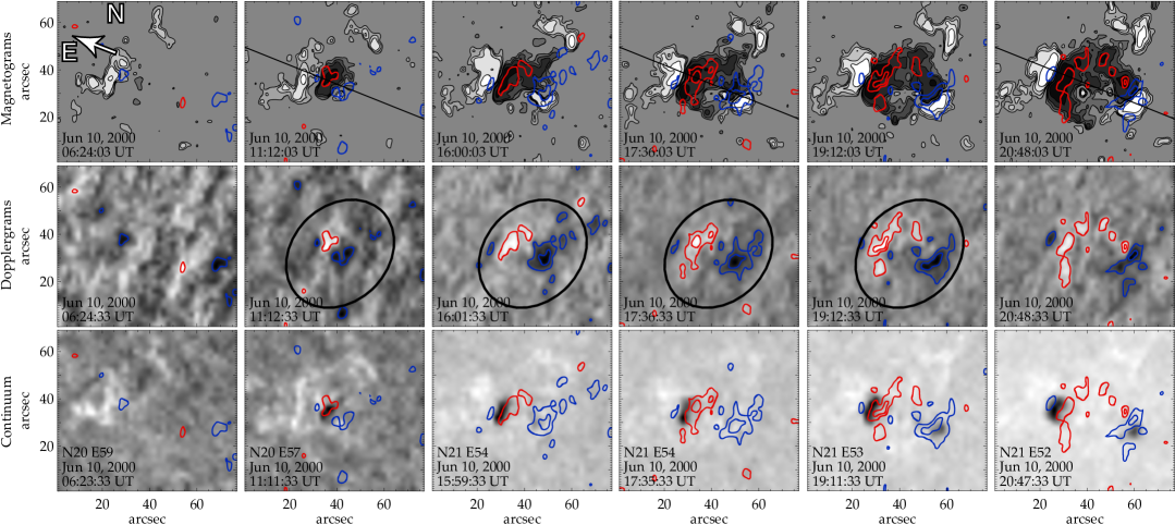
Figure 1.: The active region NOAA 9037 emerges on 10 Jun 2000 at N21 E59. On the magnetograms (isolines $\pm$60, 100, 150, 300 G), Dopplergrams, and continuum the isolines of Doppler velocities are superimposed. The blue isoline corresponds to $-$500,$-$1000  $\mathrm{m\,s^{-1}}$ – plasma motion towards the observer; the red isoline corresponds to $+$500,$+$1000  $\mathrm{m\,s^{-1}}$ – plasma motion away from the observer. Forming Doppler velocity structures are marked by an ellipse. The orientation of the images is shown in the upper left corner; the direction from the solar disk center to the emerging magnetic flux is marked by a white arrow. The black straight line on the upper-row panels marks the location of the slice of the time slice diagrams. fig:01

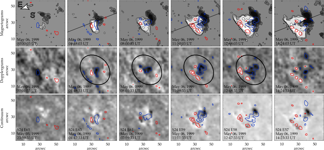
Figure 2.: Active region NOAA 8536 emerges on 6 May 1999 at S24 E65. The marking convention is the same as in Figure fig:01. fig:02

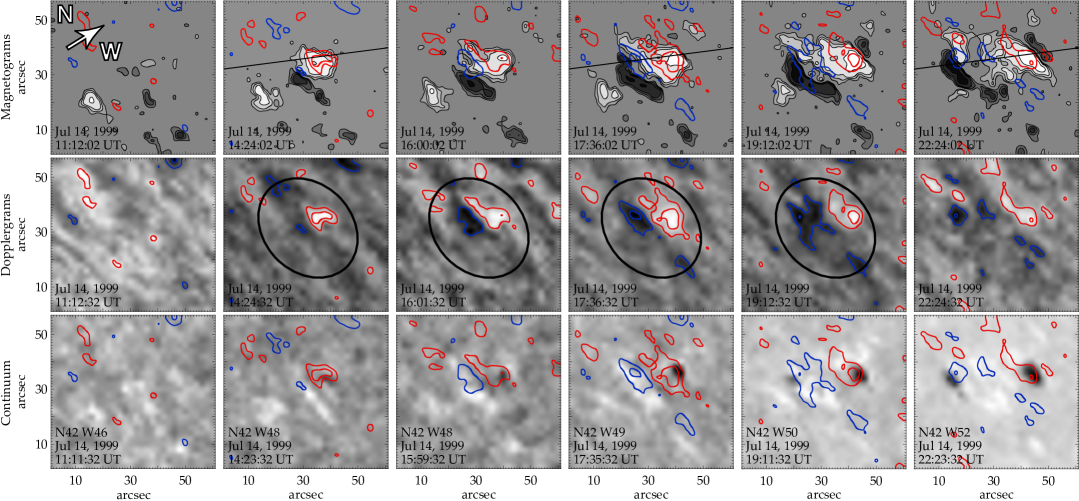
Figure 3.: Active region NOAA 8635 emerges on 14 Jul 1999 at N42 W47. The marking convention is the same as in Figure fig:01. fig:03

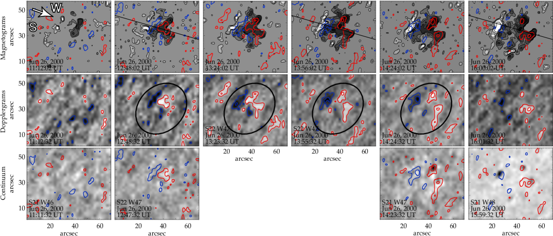
Figure 4.: Active region NOAA 9064 emerges on 26 Jun 2000 at S21 W46. The marking convention is the same as in Figure fig:01. fig:04

4 Doppler Velocity Structures

The SOHO/MDI data have a low spatial resolution which enables one to observe large-scale flows of plasma. The active regions under consideration emerge in different sectors of the solar disk, but the morphology of Doppler velocity structures during the first hours of magnetic flux emergence is similar. An amplification of negative Doppler velocities (plasma motion towards the observer) is observed on the boundary where the magnetic field changes sign located at the disk-side polarity (closer to the solar disk center) because of the projection effect of the magnetic field vector to the line of sight and of positive Doppler velocities (plasma motion away from the observer) in the limb-side polarity (closer to the solar limb) (Figures fig:01, fig:02, fig:03, and fig:04). High Doppler velocities inside the $\pm$1000  $\mathrm{m\,s^{-1}}$ isolines occupy significant areas (up to 50% of the Doppler velocity structure area inside the 500  $\mathrm{m\,s^{-1}}$ isoline within individual time intervals) that are localized in the central part of Doppler velocity structure and exist for a long time: for NOAA 9037 on June 10 at 17:36 and 19:12 UT (Figure fig:01); for NOAA 8536 on May 6 at 11:09 UT (Figure fig:02); for NOAA 8635 on July 14 at 14:24 and 17:36 UT (Figure fig:03); for NOAA 9064 on June 26 at 13:55 and 14:24 UT (Figure fig:04).

Time slice diagrams for magnetic field strength and Doppler velocities were constructed in the first hours of emergence of active regions (panels (a) and (b) in Figures fig:05, fig:06, fig:07, and fig:08). The slices are orientated along the axis of the emerging bipolar pairs, and their position is marked by a black line on the magnetograms in Figures fig:01, fig:02, fig:03, and fig:04. During the emergence of active regions a slight rotation of the axis of dipoles is observed; therefore, at the very beginning of magnetic flux emergence both polarities with Doppler velocity structures do not always fall into the slices.

The time slice diagrams clearly show that the Doppler velocity structures are located within the limits of emerging magnetic flux, and that they are not present in the surrounding regions (Figures fig:05 a, fig:06 a, fig:07 a, fig:08 a). The Doppler velocity structures form at the beginning of magnetic flux emergence, occupy an extensive region, and persist for a few hours (Figures fig:05 b, fig:06 b, fig:07 b, fig:08 b and Table tbl:dop-vel). Regions of Doppler velocities of different signs do not appear at the same time. In the first hours of magnetic flux emergence they are adjacent to each other; they then separate together with the opposite polarities.

The Doppler velocity values increase gradually and reach their peak values 4 – 12 hours after the start of the emergence of active regions, approximately at half of the velocity structure’s life time (Figures fig:05 d, fig:06 d, fig:07 d, fig:08 d). The peak values of mean Doppler velocity inside the $\pm$500  $\mathrm{m\,s^{-1}}$ isolines are 800 – 970  $\mathrm{m\,s^{-1}}$, and the peak values of maximum Doppler velocities reach 1410 – 1700  $\mathrm{m\,s^{-1}}$ (Table tbl:dop-vel). The mean Doppler velocities show the presence of velocity structures rather weakly. At the same time, as noted above, the Doppler velocities inside the $\pm$1000  $\mathrm{m\,s^{-1}}$ isolines, within individual time intervals, occupy significant areas which exist for a long time. The peak values of the Doppler velocities accompanying the emergence of active regions (Table tbl:dop-vel) substantially exceed the maximum Doppler velocities of the convective flow of the quiet Sun, which, in the SOHO/MDI data, do not exceed 1200  $\mathrm{m\,s^{-1}}$ (the points with $\theta>50^{\circ}$ in Figure 3 b of khl11).

We calculated the separation velocities of the photospheric magnetic flux outer boundaries $V_{sep}$, and estimated the contribution of magnetic flux expansion to the Doppler velocity signal $V_{exp}$ (Table tbl:sep-vel). From the comparison in Table tbl:dop-vel and Table tbl:sep-vel one can see that the Doppler velocity values observed substantially exceed the magnetic flux expansion velocity $V_{exp}$.

Previews of other active regions emerging near the limb showed that these powerful and long-lived Doppler velocity structures do not always appear. They seem to be present only in events with a high flux growth rate. khl12 has carried out a statistical investigation of 54 active regions with different spatial scales (total unsigned magnetic flux $8\times 10^{19}$ – $5\times 10^{22}$ Mx) emerging near the limb. It was found that the peak values of negative and positive Doppler velocities are related quadratically to the magnetic flux growth rate in the first hours of the emergence of active regions (Figure 6a of khl12).

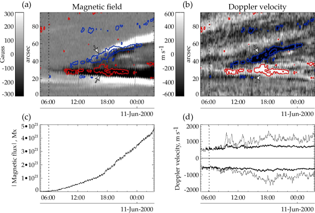
Figure 5.: Active region NOAA 9037: time slice diagrams of (a) magnetic field strength and (b) Doppler velocities. The location of the slice is marked on the magnetograms in Figure fig:01 by a black line. The blue and red isolines correspond to $-$500, $-$1000 and $+$500, $+$1000  $\mathrm{m\,s^{-1}}$, and the Doppler velocity structures analyzed are marked by arrows; (c) time variation of the total unsigned magnetic flux; (d) time variation of mean (thick line) and absolut maximum (thin line) values of negative and positive Doppler velocities in the region of emerging magnetic flux. The vertical dotted line marks the time of the beginning of magnetic flux emergence. fig:05

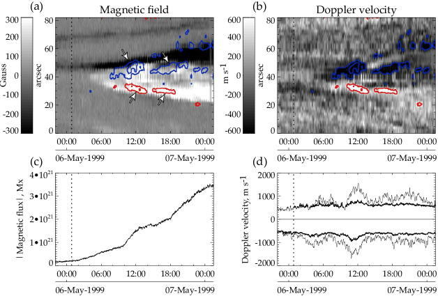
Figure 6.: Active region NOAA 8536: time slice diagrams of (a) magnetic field strength and (b) Doppler velocities. The location of the slice is marked on the magnetograms in Figure fig:02 by a black line. The marking convention is the same as in Figure fig:05. fig:06

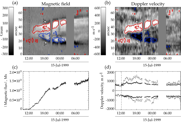
Figure 7.: Active region NOAA 8635: time slice diagrams of (a) magnetic field strength and (b) Doppler velocities. The location of the slice is marked on the magnetograms in Figure fig:03 by a black line. The marking convention is the same as in Figure fig:05. fig:07

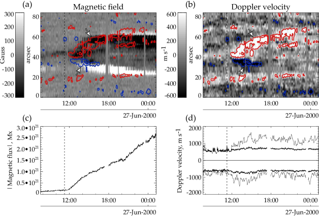
Figure 8.: Active region NOAA 9064: time slice diagrams of (a) magnetic field strength and (b) Doppler velocities. The location of the slice is marked on the magnetograms in Figure fig:04 by a black line. The marking convention is the same as in Figure fig:05. fig:08

Active	Negative Doppler velocities				Positive Doppler velocities
regions	$\bf V_{mean-},$	$\bf V_{max-},$	d, 1	t,	$\bf V_{mean+},$	$\bf V_{max+},$	d, 1	t,
	$\bf m\,s^{-1}$	$\bf m\,s^{-1}$	Mm	h	$\bf m\,s^{-1}$	$\bf m\,s^{-1}$	Mm	h
9037	$-$810	$-$1640	14	15	850	1630	15	13
8536	$-$970	$-$1700	18	14	830	1560	10	9
8635	$-$830	$-$1410	16.5	10	960	1660	15	13.5
9064	$-$800	$-$1520	9	4.5	810	1650	16	10

¹Size of Doppler velocity structure inside the isoline $-$500 or $+$500  $\mathrm{m\,s^{-1}}$ along the slices
in Figures fig:05  b, fig:06  b, fig:07  b, fig:08  b taking into account the projection effect.

Table 2.: Peak values of mean and absolut maximum Doppler velocities ($V_{mean-}$, $V_{max-}$, $V_{mean+}$, $V_{max+}$), size ($d$), and life time ($t$) of the velocity structures during the first hours of the emergence of active regionstbl:dop-vel

Active	Time interval	$\bf\overrightarrow{V}_{sep},$	$\bf V_{exp},$
regions		$\bf m\,s^{-1}$	$\bf m\,s^{-1}$
9037	10 Jun 2000, 17:10 – 19:10 UT	450	$\lesssim$ 370
8536	06 May 1999, 10:05 – 12:05 UT	150	$\lesssim$ 130
8635	14 Jul 1999, 17:00 – 19:00 UT	340	$\lesssim$ 290
9064	26 Jun 2000, 14:00 – 16:00 UT	820	$\lesssim$ 660

Table 3.: The mean relative separation velocities of the photospheric magnetic flux outer boundaries ($\overrightarrow{V}_{sep}$), the contribution of the magnetic flux expansion to the line of sight signal of Doppler velocity ($V_{exp}$), and the periods of time (Time intervals) for which $\overrightarrow{V}_{sep}$ and $V_{exp}$ were determinedtbl:sep-vel

5 Geometrical Asymmetry of Emerging Magnetic Flux

During the appearance of active regions it is possible to see the well-known geometrical asymmetry of emerging magnetic flux (dri90 and references therein). It appears that sunspots of leading polarity move away from the location of the emergence much faster than those of following polarity do. In the time slice diagrams of the magnetic field of the active regions under consideration, the following polarity is situated at the bottom, and the leading one at the top (Figures fig:05 a, fig:06 a, fig:07 a, fig:08 a). In NOAA 9037, soon after emergence, the following (negative) polarity is set against the existing concentration of the positive magnetic field and stops drifting, while the leading polarity moves along the slice at high velocity (Figure fig:05 a). NOAA 8536 emerges before an existing concentration of negative magnetic field. Therefore, the following polarity moves faster than the leading one in the first hours of emergence, but then the leading polarity begins to move with greater velocity (Figure fig:06 a). In NOAA 8635 and 9064, emerging at the W-limb, it is clearly seen that the leading polarity moves considerably faster than the following one (Figures fig:07 a and fig:08 a).

Figure 9.: The time variation for the difference between the positive and negative Doppler velocities for mean (thick line) and maximal (thin line) values in the studied active regions. The polarities of the locations of the positive and negative Doppler velocities are marked on the plots. fig:09

6 Asymmetry in the Doppler Velocity Fields

Asymmetry is also observed in the Doppler velocity fields. In the time slice diagrams in Figures fig:05 a, fig:06 a, fig:07 a, fig:08 a, one can clearly see that the Doppler velocity structures located at the region of the leading magnetic polarity are more powerful and exist longer than in the following one.

We performed a quantitative analysis for the Doppler velocity asymmetry. Figures fig:09 presents the plots of time variation for the difference between the positive and negative Doppler velocities for mean and maximal values. There are some blanks in the mean Doppler velocity asymmetry for those time instants when the velocities in the region of emerging magnetic flux were less than 500  $\mathrm{m\,s^{-1}}$. For active regions NOAA 8536 and 8635 emerging near different limbs, a well-defined dominance of the Doppler velocities located in the leading polarity is observed during the first 12 hours of the emergence. In two other active regions, NOAA 9037 and NOAA 9064, also emerging near different limbs, the asymmetry value changes its sign. The NOAA 9037 appearance starts with the emergence of a magnetic loop whose axis is oriented almost perpendicularly to the line of sight. Its rise is accompanied by a dominance of the negative Doppler velocity. Approximately from 09:00 UT, a magnetic flux emergence appears whose axis is oriented along the line of sight. Against this background, one observes a significant dominance of the positive Doppler velocities localized in the following polarity. In the NOAA 9064 early emergence, the mean Doppler velocity values show practically no asymmetry, but one observes a dominance of the maximal negative Doppler velocities corresponding to the following polarity. Approximately three hours after the start of emergence, the asymmetry value changes sign, and a noticeable dominance of the positive Doppler velocity localized in the leading polarity begins.

In all the active regions under consideration, the Doppler velocity asymmetry reaches its peak value soon after the start of magnetic flux emergence, and then gradually drops within 7 – 12 hours. The Doppler velocity asymmetry decreasing time is comparable to the lifetime of the velocity structures. The peak values of asymmetry for the mean and maximal Doppler velocities reach 240 – 460  $\mathrm{m\,s^{-1}}$ and 710 – 940  $\mathrm{m\,s^{-1}}$, respectively.

7 Interpretation of the Results

Let us consider the contribution of possible motions to the line of sight Doppler velocity signal in data with low spatial resolution (Figure fig:10 a).

i) The magnetic flux rise velocity $\overrightarrow{V}_{up}$. $\overrightarrow{V}_{up}$ should have a similar contribution in the leading and following polarities. When active regions emerge near the solar disk center, the maximum values of the upflow Doppler velocities reach $\overrightarrow{V}_{up}\sim$300 – 1000  $\mathrm{m\,s^{-1}}$ (Figure 4 of khl12 and references in Section 1 of this paper). The projection of these velocities to the line of sight at the heliocentric angle $\theta$ = $60^{\circ}$ will be $V_{up}\lesssim$150 – 500  $\mathrm{m\,s^{-1}}$.

ii) The plasma downflow velocity $\overrightarrow{V}_{down}$. In the active regions emerging near the solar disk center, at the footpoints of the magnetic loops, one observes positive Doppler velocities interpreted as a downflow of plasma being carried out into the solar atmosphere (see references in Section 1 of this paper). The plasma downflow takes place along the magnetic field lines. Theoretical models show that the velocities of draining plasma have a significant horizontal component at the beginning of the magnetic flux emergence (e.g., shi90, arch04, tor10, tor11).

iii) The magnetic flux horizontal expansion velocity $\overrightarrow{V}_{exp}$. $\overrightarrow{V}_{exp}$ should have a similar contribution in the leading and the following polarities under the condition of equality of their gas pressure. From the theory of magnetic flux emergence into the solar atmosphere, an inverse relation exists between the expansion velocities and degree of twist of the emerging magnetic flux (see, for example, mur06). che10 showed that an emerging tube with a total toroidal flux content of $7.6\times 10^{21}$ Mx creates a transient pressure excess that results in diverging horizontal flows with velocities over 3  $\mathrm{km\,s^{-1}}$ for approximately five hours. In this case, the plasma flow velocities are comparable to the separation velocities of the photospheric magnetic flux outer boundaries. The observations show that at the very beginning of the emergence the magnetic flux expansion has a maximal velocity that then drops rapidly with time. Even at the emergence of the powerful active region NOAA 10488, with a total unsigned magnetic flux at the maximum evolution of $>6\times 10^{22}$ Mx and a total unsigned magnetic flux growth rate during the first hours of $4.1\times 10^{20}$ Mx h^-1, the separation velocities of the photospheric magnetic flux outer boundaries had already dropped to 0.3  $\mathrm{km\,s^{-1}}$ two hours after the beginning of the emergence [Grigor’ev, Ermakova, and Khlystova (2009)].

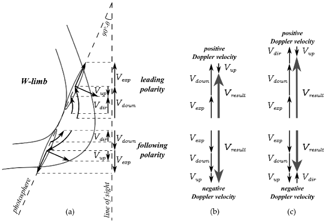
Figure 10.: (a) The simple scheme of the plasma flows accompanying the emergence of the magnetic flux near the W-limb. The velocity vectors of the possible flows and their projection to the line of sight in the leading and following polarities are marked by arrows. $V_{up}$ is the magnetic flux rise velocity; $V_{down}$ is the plasma downflow velocity being carried out into the solar atmosphere by the emerging magnetic flux; $V_{exp}$ is the magnetic flux horizontal expansion velocity; $V_{dir}$ is the plasma directional flow velocity inside the emerging magnetic structure (in this case from the following polarity to the leading one). (b) The compositional result of the velocity components along the line of sight without the plasma directional flow $V_{dir}$. (c) The compositional result of the velocity components along the line of sight taking into account the plasma directional flow $V_{dir}$. fig:10

iv) It is possible that plasma directional flows exist inside the emerging magnetic structure $\overrightarrow{V}_{dir}$. Directional flows, as well as the plasma downflow $\overrightarrow{V}_{down}$, take place along the magnetic field lines. Searches for such flows in the Doppler velocity asymmetry between the leading and following polarities in the active regions emerging near the solar disk center did not provide consistent results [Cauzzi, Canfield, and Fisher (1996), Sigwarth, Schmidt, and Schuessler (1998), Chapman (2002), Pevtsov and Lamb (2006), Battiato et al. (2006), Grigor’ev, Ermakova, and Khlystova (2011)]. Plasma flows are theoretically expected to be directed from the leading polarity into the following one. The thin flux tube theory shows that these flows are due to the Coriolis force acting on the emerging magnetic structure, and the velocities of these flows reach some hundreds of meters per second (for a detailed analysis, see fan09). However, when entering the convection zone high layers (20 – 30 Mm under the photosphere), the magnetic flux undergoes a strong expansion and fragmentation. Therefore, the probability of conservation of the flows caused by the Coriolis force is not known. The models of the magnetic flux emergence from the near-surface layers into the solar atmosphere do not consider the existence of these flows. It is also possible that plasma flows occur from the following polarity into the leading one. A discussion of the mechanisms leading to their origin may be found in cau96.

Thus, the line of sight Doppler velocity signal in data with low spatial resolution contains contributions from the following flows (Figure fig:10 a):

$$\overrightarrow{V}=\overrightarrow{V}_{up}+\overrightarrow{V}_{down}+\overrightarrow{V}_{exp}+\overrightarrow{V}_{dir},$$ (5)

Their projections onto the line of sight in the positive and negative Doppler velocity structures are determined as:

$$V_{-}=+\overrightarrow{V}_{up}cos\theta+\overrightarrow{V}_{down}cosX_{1}+\overrightarrow{V}_{exp}sin\theta\pm\overrightarrow{V}_{dir}cosX_{1},$$ (6)

$$V_{+}=-\overrightarrow{V}_{up}cos\theta+\overrightarrow{V}_{down}cosX_{2}+\overrightarrow{V}_{exp}sin\theta\pm\overrightarrow{V}_{dir}cosX_{2},$$ (7)

where $\theta$ is the heliocentric angle, and $X_{1}$ and $X_{2}$ are the angles between the line of sight and the magnetic field lines in the polarities where the negative and positive velocity structures are localized.

In the velocity structures accompanying the emergence of active regions under consideration, one observes high Doppler velocities that reach their peak values 4 – 12 hours after the magnetic flux emergence begins (Figures fig:05 d, fig:06 d, fig:07 d, fig:08 d). Doppler velocities more than 1000  $\mathrm{m\,s^{-1}}$ concentrate in the central part of the velocity structures, occupy significant areas, and exist over long time intervals (Figures fig:01, fig:02, fig:03, and fig:04). Let us discuss what the observed velocities are associated with, having considered the contribution of possible motions to the line of sight Doppler velocity signal at the heliocentric angle $\theta=60^{\circ}$. The maximal contribution of the magnetic flux rise velocities should be $V_{up}$ $\sim$ 150 – 500  $\mathrm{m\,s^{-1}}$, with a mean contribution of 300  $\mathrm{m\,s^{-1}}$. The contribution of the magnetic flux horizontal expansion velocities to our active regions is $V_{exp}$ $\sim$ 130 – 660  $\mathrm{m\,s^{-1}}$ (Table tbl:sep-vel). The velocity of directional flow $\overrightarrow{V}_{dir}$ will determine the value of the Doppler velocity asymmetry between the velocity structures of opposite sign and, for active regions NOAA 9037 and 8536, 12 hours after the start of emergence it has no contribution. Thus, one can see that the high Doppler velocities are caused by the significant component of the plasma downflow velocities $\overrightarrow{V}_{down}$ (Figure fig:10 b).

The Doppler velocity asymmetry between velocity structures of the leading and following polarities reaches its peak values soon after the emergence begins, and then it gradually drops (Figure fig:09). In two active regions, NOAA 8536 and 8635, emerging near different limbs, one observes an explicit dominance of the Doppler velocities localized in the leading polarity. In two other active regions, NOAA 9037 and 9064, also emerging near different limbs, the Doppler velocity asymmetry value changes sign, but, at individual time intervals, there is a Doppler velocity dominance in the following polarity. There is probably a contribution from the plasma directional flow $V_{dir}$ (Figure fig:10 c). The Doppler velocity asymmetry may be caused by a morphological asymmetry of active regions that becomes apparent because the magnetic flux of the leading polarity is more compact than of the following one. However, to better understand the causes for the asymmetry between Doppler velocity structures, one should search for some additional relations.

8 Conclusion

S-Conclusion

Analysis of photospheric flows accompanying the emergence of active regions near the limb showed the existence of an extensive region of enhanced negative Doppler velocities on the boundary where the magnetic field changes sign, which is located in the polarity closer to the solar disk center because of the projection effect. The region of positive Doppler velocities is adjacent to it in the magnetic polarity closer to the solar limb. The observed flows form at the start of active region emergence and are present for a few hours. The Doppler velocity values increase gradually and reach their peak values 4 – 12 hours after the start of the magnetic flux emergence. The peak values of the mean (inside the $\pm$500  $\mathrm{m\,s^{-1}}$ isolines) and maximum Doppler velocities are 800 – 970  $\mathrm{m\,s^{-1}}$ and 1410 – 1700  $\mathrm{m\,s^{-1}}$, respectively. The Doppler velocity values observed substantially exceed the separation velocities of the photospheric magnetic flux outer boundaries and most likely are caused by a significant component of the plasma downflow velocities being carried out into the solar atmosphere by emerging magnetic flux.

An asymmetry was detected between the velocity structures of the leading and following polarities. Doppler velocity structures located in a region of leading magnetic polarity are more powerful and exist longer than those in a region of following magnetic polarity. The Doppler velocity asymmetry between velocity structures of the leading and following polarities reaches peak values soon after emergence begins and then gradually drops within 7 – 12 hours. The peak values of asymmetry for the mean and maximal Doppler velocities reach 240 – 460  $\mathrm{m\,s^{-1}}$ and 710 – 940  $\mathrm{m\,s^{-1}}$, respectively. Additional investigations are necessary to understand the reasons for the Doppler velocity asymmetry. However, it could be caused by the plasma directional flows inside the emerging magnetic structure or morphological asymmetry between the leading and following polarities.

Acknowledgements

The author expresses sincere gratitude to the Geuest Editor for useful comments. The author is grateful to Prof. V.M. Grigoriev, L.V. Ermakova, and V.G. Eselevich for important suggestions and help in understanding the obtained results. This work used data obtained by the SOHO/MDI instrument. SOHO is a mission of international cooperation between ESA and NASA. The MDI is a project of the Stanford-Lockheed Institute for Space Research. This study was supported by RFBR grants 10-02-00607-a, 10-02-00960-a, 11-02-00333-a, 12-02-00170-a, state contracts of the Ministry of Education and Science of the Russian Federation Nos. 02.740.11.0576 and 16.518.11.7065, the program of the Division of Physical Sciences of the Russian Academy of Sciences No. 16, the Integration Project of SB RAS No. 13, and the program of the Presidium of Russian Academy of Sciences No. 22.

References

- Archontis et al. (2004) Archontis, V., Moreno-Insertis, F., Galsgaard, K., Hood, A., O’Shea, E.: 2004, Emergence of magnetic flux from the convection zone into the corona. A&A 426, 1047 – 1063. doi:10.1051/0004-6361:20035934.
- Bachmann (1978) Bachmann, G.: 1978, On the evolution of magnetic and velocity fields of an originating sunspot group. Bulletin of the Astronomical Institutes of Czechoslovakia 29, 180 – 184.
- Barth and Livi (1990) Barth, C.S., Livi, S.H.B.: 1990, Magnetic Bipoles in Emerging Flux Regions on the Sun. Rev. Mex. Astron. Astrofis. 21, 549.
- Battiato et al. (2006) Battiato, V., Billotta, S., Contarino, L., Guglielmino, S., Romano, P., Soadaro, D., Zuccarello, F.: 2006, High Resolution Observations of Emerging Active Regions Carried Out at the THEMIS Telescope. In: SOHO-17. 10 Years of SOHO and Beyond, ESA Special Publication 617.
- Brants (1985a) Brants, J.J.: 1985a, High-resolution spectroscopy of active regions. II Line-profile interpretation, applied to an emerging flux region. Sol. Phys. 95, 15 – 36. doi:10.1007/BF00162633.
- Brants (1985b) Brants, J.J.: 1985b, High-resolution spectroscopy of active regions. III - Relations between the intensity, velocity, and magnetic structure in an emerging flux region. Sol. Phys. 98, 197 – 217. doi:10.1007/BF00152456.
- Brants and Steenbeek (1985) Brants, J.J., Steenbeek, J.C.M.: 1985, Morphological evolution of an emerging flux region. Sol. Phys. 96, 229 – 252. doi:10.1007/BF00149682.
- Cauzzi, Canfield, and Fisher (1996) Cauzzi, G., Canfield, R.C., Fisher, G.H.: 1996, A Search for Asymmetric Flows in Young Active Regions. ApJ 456, 850 – 860. doi:10.1086/176702.
- Chapman (2002) Chapman, G.A.: 2002, A Study of AR 9144; A Fast-Growing EFR. Sol. Phys. 209, 141 – 152. doi:10.1023/A:1020994131849.
- Cheung et al. (2010) Cheung, M.C.M., Rempel, M., Title, A.M., Schüssler, M.: 2010, Simulation of the Formation of a Solar Active Region. ApJ 720, 233 – 244. doi:10.1088/0004-637X/720/1/233.
- Chou and Wang (1987) Chou, D., Wang, H.: 1987, The separation velocity of emerging magnetic flux. Sol. Phys. 110, 81 – 99. doi:10.1007/BF00148204.
- Fan (2009) Fan, Y.: 2009, Magnetic Fields in the Solar Convection Zone. Living Reviews in Solar Physics 6, 4.
- Frazier (1972) Frazier, E.N.: 1972, The Magnetic Structure of Arch Filament Systems. Sol. Phys. 26, 130 – 141. doi:10.1007/BF00155113.
- Gopasyuk (1967) Gopasyuk, S.I.: 1967, The velocity field in an active region at spot appearance stag. Izvestiya Ordena Trudovogo Krasnogo Znameni Krymskoj Astrofizicheskoj Observatorii 37, 29 – 43.
- Gopasyuk (1969) Gopasyuk, S.I.: 1969, The velocity field on the two levels in the active region of July 1966. Izvestiya Ordena Trudovogo Krasnogo Znameni Krymskoj Astrofizicheskoj Observatorii 40, 111 – 126.
- Grigor’ev, Ermakova, and Khlystova (2007) Grigor’ev, V.M., Ermakova, L.V., Khlystova, A.I.: 2007, Dynamics of line-of-sight velocities and magnetic field in the solar photosphere during the formation of the large active region NOAA 10488. Astronomy Letters 33, 766 – 770. doi:10.1134/S1063773707110072.
- Grigor’ev, Ermakova, and Khlystova (2009) Grigor’ev, V.M., Ermakova, L.V., Khlystova, A.I.: 2009, Emergence of magnetic flux at the solar surface and the origin of active regions. Astron. Rep. 53, 869 – 878. doi:10.1134/S1063772909090108.
- Grigor’ev, Ermakova, and Khlystova (2011) Grigor’ev, V.M., Ermakova, L.V., Khlystova, A.I.: 2011, The dynamics of photospheric line-of-sight velocities in emerging active regions. Astronomy Reports 55, 163 – 173. doi:10.1134/S1063772911020041.
- Guglielmino et al. (2006) Guglielmino, S.L., Martínez Pillet, V., Ruiz Cobo, B., Zuccarello, F., Lites, B.W.: 2006, A Detailed Analysis of an Ephemeral Region . Memorie della Societa Astronomica Italiana Supplementi 9, 103 – 105.
- Hagenaar (2001) Hagenaar, H.J.: 2001, Ephemeral Regions on a Sequence of Full-Disk Michelson Doppler Imager Magnetograms. ApJ 555, 448 – 461. doi:10.1086/321448.
- Harvey and Martin (1973) Harvey, K.L., Martin, S.F.: 1973, Ephemeral Active Regions. Sol. Phys. 32, 389 – 402. doi:10.1007/BF00154951.
- Kawaguchi and Kitai (1976) Kawaguchi, I., Kitai, R.: 1976, The velocity field associated with the birth of sunspots. Sol. Phys. 46, 125 – 135. doi:10.1007/BF00157559.
- Khlystova (2011) Khlystova, A.: 2011, Center-limb dependence of photospheric velocities in regions of emerging magnetic fields on the Sun. A&A 528, A7. doi:10.1051/0004-6361/201015765.
- Khlystova (2012) Khlystova, A.: 2012, The Relationship between Plasma Flow Velocities and Magnetic Field Parameters During the Emergence of Active Regions at the Solar Photospheric Level. Sol. Phys., in Topical Issue “Advances of European Solar Physics”. doi:10.1007/s11207-012-0193-4.
- Kozu, Kitai, and Funakoshi (2005) Kozu, H., Kitai, R., Funakoshi, Y.: 2005, Development of Real-Time Frame Selector 2 and the Characteristic Convective Structure in the Emerging Flux Region. PASJ 57, 221 – 234.
- Kozu et al. (2006) Kozu, H., Kitai, R., Brooks, D.H., Kurokawa, H., Yoshimura, K., Berger, T.E.: 2006, Horizontal and Vertical Flow Structure in Emerging Flux Regions. PASJ 58, 407 – 421.
- Kubo, Shimizu, and Lites (2003) Kubo, M., Shimizu, T., Lites, B.W.: 2003, The Evolution of Vector Magnetic Fields in an Emerging Flux Region. ApJ 595, 465 – 482. doi:10.1086/377333.
- Lagg et al. (2007) Lagg, A., Woch, J., Solanki, S.K., Krupp, N.: 2007, Supersonic downflows in the vicinity of a growing pore. Evidence of unresolved magnetic fine structure at chromospheric heights. A&A 462, 1147 – 1155. doi:10.1051/0004-6361:20054700.
- Lites, Skumanich, and Martinez Pillet (1998) Lites, B.W., Skumanich, A., Martinez Pillet, V.: 1998, Vector magnetic fields of emerging solar flux. I. Properties at the site of emergence. A&A 333, 1053 – 1068.
- Luoni et al. (2011) Luoni, M.L., Démoulin, P., Mandrini, C.H., van Driel-Gesztelyi, L.: 2011, Twisted Flux Tube Emergence Evidenced in Longitudinal Magnetograms: Magnetic Tongues. Sol. Phys. 270, 45 – 74. doi:10.1007/s11207-011-9731-8.
- Murray et al. (2006) Murray, M.J., Hood, A.W., Moreno-Insertis, F., Galsgaard, K., Archontis, V.: 2006, 3D simulations identifying the effects of varying the twist and field strength of an emerging flux tube. A&A 460, 909 – 923. doi:10.1051/0004-6361:20065950.
- Otsuji et al. (2011) Otsuji, K., Kitai, R., Ichimoto, K., Shibata, K.: 2011, Statistical Study on the Nature of Solar-Flux Emergence. PASJ 63, 1047 – 1057.
- Pevtsov and Lamb (2006) Pevtsov, A., Lamb, J.B.: 2006, Plasma Flows in Emerging Sunspots in Pictures. In: Leibacher, J., Stein, R.F., Uitenbroek, H. (eds.) Solar MHD Theory and Observations: A High Spatial Resolution Perspective, Astronomical Society of the Pacific Conference Series 354, 249 – 255.
- Scherrer et al. (1995) Scherrer, P.H., Bogart, R.S., Bush, R.I., Hoeksema, J.T., Kosovichev, A.G., Schou, J., Rosenberg, W., Springer, L., Tarbell, T.D., Title, A., Wolfson, C.J., Zayer, I., MDI Engineering Team: 1995, The Solar Oscillations Investigation - Michelson Doppler Imager. Sol. Phys. 162, 129 – 188. doi:10.1007/BF00733429.
- Schoolman (1973) Schoolman, S.A.: 1973, Videomagnetograph Studies of Solar Magnetic Fields. II: Field Changes in an Active Region. Sol. Phys. 32, 379 – 388. doi:10.1007/BF00154950.
- Shibata et al. (1990) Shibata, K., Nozawa, S., Matsumoto, R., Sterling, A.C., Tajima, T.: 1990, Emergence of solar magnetic flux from the convection zone into the photosphere and chromosphere. ApJ 351, L25 – L28. doi:10.1086/185671.
- Sigwarth, Schmidt, and Schuessler (1998) Sigwarth, M., Schmidt, W., Schuessler, M.: 1998, Upwelling in a young sunspot. A&A 339, L53 – L56.
- Snodgrass (1983) Snodgrass, H.B.: 1983, Magnetic rotation of the solar photosphere. ApJ 270, 288 – 299. doi:10.1086/161121.
- Solanki et al. (2003) Solanki, S.K., Lagg, A., Woch, J., Krupp, N., Collados, M.: 2003, Three-dimensional magnetic field topology in a region of solar coronal heating. Nature 425, 692 – 695. doi:10.1038/nature02035.
- Strous and Zwaan (1999) Strous, L.H., Zwaan, C.: 1999, Phenomena in an Emerging Active Region. II. Properties of the Dynamic Small-Scale Structure. ApJ 527, 435 – 444. doi:10.1086/308071.
- Strous et al. (1996) Strous, L.H., Scharmer, G., Tarbell, T.D., Title, A.M., Zwaan, C.: 1996, Phenomena in an emerging active region. I. Horizontal dynamics. A&A 306, 947 – 959.
- Tarbell et al. (1989) Tarbell, T.D., Topka, K., Ferguson, S., Frank, Z., Title, A.M.: 1989, High - resolution observations of emerging magnetic flux. In: O. von der Luehe (ed.) High spatial resolution solar observations, 506 – 520.
- Toriumi and Yokoyama (2010) Toriumi, S., Yokoyama, T.: 2010, Two-step Emergence of the Magnetic Flux Sheet from the Solar Convection Zone. ApJ 714, 505 – 516. doi:10.1088/0004-637X/714/1/505.
- Toriumi et al. (2011) Toriumi, S., Miyagoshi, T., Yokohama, T., Isobe, H., Shibata, K.: 2011, Dependence of the Magnetic Energy of Solar Active Regions on the Twist Intensity of the Initial Flux Tubes. PASJ 63, 407 – 415.
- van Driel-Gesztelyi and Petrovay (1990) van Driel-Gesztelyi, L., Petrovay, K.: 1990, Asymmetric flux loops in active regions. Sol. Phys. 126, 285 – 298. doi:10.1007/BF00153051.
- Xu, Lagg, and Solanki (2010) Xu, Z., Lagg, A., Solanki, S.K.: 2010, Magnetic structures of an emerging flux region in the solar photosphere and chromosphere. A&A 520, A77. doi:10.1051/0004-6361/200913227.
- Zwaan, Brants, and Cram (1985) Zwaan, C., Brants, J.J., Cram, L.E.: 1985, High-resolution spectroscopy of active regions. I - Observing procedures. Sol. Phys. 95, 3 – 14. doi:10.1007/BF00162632.