Adaptive Wavelet Collocation Method
for Simulation of Time Dependent Maxwell’s Equations

Abstract

This paper investigates an adaptive wavelet collocation time domain method for the numerical solution of Maxwell’s equations. In this method a computational grid is dynamically adapted at each time step by using the wavelet decomposition of the field at that time instant. In the regions where the fields are highly localized, the method assigns more grid points; and in the regions where the fields are sparse, there will be less grid points. On the adapted grid, update schemes with high spatial order and explicit time stepping are formulated. The method has high compression rate, which substantially reduces the computational cost allowing efficient use of computational resources. This adaptive wavelet collocation method is especially suitable for simulation of guided-wave optical devices.

keyword: Maxwell’s equations, time domain methods, wavelets, wavelet collocation method, adaptivity

1 Introduction

The numerical solution of Maxwell’s equations is an active area of computational research. Typically, Maxwell’s equations are solved either in the frequency domain or in the time domain, where each of these approaches has its own relative merits. We are specifically interested in efficient algorithms for light propagation problems in guided wave photonic applications [1], and work in the time domain. The most popular class of methods in this area is the finite difference time domain (FDTD) method [2]. Due to the structured grid requirement of these methods, they become cumbersome while dealing with optical devices having curved interfaces and different length scales. To overcome these difficulties, a discontinuous Galerkin time domain (DGTD) method has been investigated [3]. For a time dependent wave propagation problem, all these methods use a fixed grid/mesh for discretization. In general, such a grid can under-sample the temporal dynamics, or over-sample the field propagation causing high computational costs. If the spatial grid adapts itself according to the temporal evolution of the field, then the computational resources will be used much more efficiently.

We propose an adaptive-grid method which represents propagating fields at each time step by a compressed wavelet decomposition, and which automatically adapts the computational mesh to the changing shape of the signal. In the initial studies of the wavelet formulation, the interpolating scaling functions were used for frequency domain waveguide analysis [4]. To the best of our knowledge, the suitability of the wavelet decompositions for time dependent Maxwell problems has not yet been investigated. Vasilyev and his co-authors developed the adaptive wavelet collocation time domain (AWC-TD) method as a general scheme to solve evolution equations, and they successfully verified the scheme’s effectiveness in the area of computational fluid dynamics [5, 6]. Based on these studies, we present in this work a proof-of-concept for an AWC-TD for the time dependent Maxwell’s equations.

The paper is organized as follows. In Sec. 2, we provide a brief account on Maxwell’s equations and some of the related concepts for their numerical solutions. We start Sec. 3 with an introduction to (interpolating) wavelets, and how they can be used to discretize partial differential equations. Also in this section we explain the structure of AWC-TD method in the context of Maxwell’s equations. Sec. 4 gives algorithmic details of the method. Numerical results of the AWC-TD method are given in Sec. 5 which contains our numerical experiments of propagating a 2D Gaussian peak in homogeneous environment. Finally we close the paper with concluding remarks in Sec. 6.

2 Time domain Maxwell’s equations

Propagation of optical waves in a linear, non-magnetic dielectric medium with no charges and currents is governed by the following time dependent Maxwell’s equations

$$-\dfrac{\partial}{\partial t}\vec{\mathcal{B}}(\vec{r},t)=\nabla\times\vec{\mathcal{E}}(\vec{r},t),\quad\dfrac{\partial}{\partial t}\vec{\mathcal{D}}(\vec{r},t)=\nabla\times\vec{\mathcal{H}}(\vec{r},t),\quad\nabla\cdot\vec{\mathcal{D}}(\vec{r},t)=0,\ \text{ and }\ \nabla\cdot\vec{\mathcal{B}}(\vec{r},t)=0,$$ (1)

where the electric field $\vec{\mathcal{E}}$ and the electric flux density $\vec{\mathcal{D}}$, as well as the magnetic field $\vec{\mathcal{H}}$ and the magnetic flux density $\vec{\mathcal{B}}$, are related by the constitutive relations

$$\vec{\mathcal{D}}(\vec{r},t)=\varepsilon_{0}\varepsilon_{r}(\vec{r})\vec{\mathcal{E}}(\vec{r},t)\ \text{ and }\ \vec{\mathcal{B}}(\vec{r},t)=\mu_{0}\vec{\mathcal{H}}(\vec{r},t).$$

Here $\varepsilon_{0}$ is the free space permittivity, $\varepsilon_{r}$ is the relative permittivity and $\mu_{0}$ is free space permeability.

For illustration purpose, we restrict ourselves to a 2D setting where the fields and the material properties are assumed to be invariant in the $y$-direction, i. e. $\vec{r}=(x,z)$ and the partial derivatives of all fields with respect to $y$ vanish identically. We suppress the explicit function dependence on $\vec{r}$ and $t$. Then Maxwell’s equations (1) decouple into a pair of independent sets of equations,

$$\frac{\partial\mathcal{E}_{x}}{\partial t}=-\frac{1}{\varepsilon_{0}\varepsilon_{r}}\frac{\partial\mathcal{H}_{y}}{\partial z},~{}\hfill\frac{\partial\mathcal{E}_{z}}{\partial t}=\frac{1}{\varepsilon_{0}\varepsilon_{r}}\frac{\partial\mathcal{H}_{y}}{\partial x},~{}\hfill\frac{\partial\mathcal{H}_{y}}{\partial t}=\frac{1}{\mu_{0}}\left(\frac{\partial\mathcal{E}_{x}}{\partial z}-\frac{\partial\mathcal{E}_{z}}{\partial x}\right),$$ (2)

identified as transverse electric (TE)_y setting, and

$$\frac{\partial\mathcal{H}_{x}}{\partial t}=\frac{1}{\mu_{0}}\frac{\partial\mathcal{E}_{y}}{\partial z},~{}\hfill\quad\frac{\partial\mathcal{H}_{z}}{\partial t}=-\frac{1}{\mu_{0}}\frac{\partial\mathcal{E}_{y}}{\partial x},~{}\hfill\frac{\partial\mathcal{E}_{y}}{\partial t}=\frac{1}{\varepsilon_{0}\varepsilon_{r}}\left(\frac{\partial\mathcal{H}_{x}}{\partial z}-\frac{\partial\mathcal{H}_{z}}{\partial x}\right),$$ (3)

identified as transverse magnetic (TM)_y setting. Here $\mathcal{E}_{x}$, $\mathcal{E}_{z}$, $\cdots$ etc. denote the respective field components.

Originally, Maxwell’s equations are formulated for a whole space. For numerical computations we need to restrict them to a bounded computational domain $\Omega$ as shown in Fig. 1. This is done with a transparent boundary condition, which is realized in our case with perfectly matched layer (PML) [7, 8]. The principle of PML is that (outgoing) waves scattered from the scatterer $\Omega_{\mathrm{s}}$ pass through the interface between $\Omega$ and PML without reflections, and attenuate significantly inside the PML. The waves virtually vanish before reaching the outermost boundary of the PML, where the perfectly electric boundary (PEB) condition is employed. Implementation details about the PML technique specific for the method discussed in this paper can be found in Ref. [9]. For the sake of clarity, we work with the general formulation given by Eq. (2)-(3).

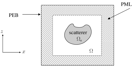
Figure 1: Typical simulation setting with a computational domain $\Omega$ surrounded by the perfectly matched layer. Here just for the sake of illustration, we show the scatterer $\Omega_{\rm{s}}$ completely enclosed inside $\Omega$. Other configurations like incoming-outgoing waveguides are also possible [9].

As in the case of the standard FDTD method [2], in our approach we use the central difference scheme for the time derivatives in Eq. (2)-(3), but we will construct a different discretization scheme of the spatial derivatives. This is done with interpolating scaling functions and lifted interpolating wavelets (explained in Sec. 3). The induced multiresolution approximation [10, 11] enables us to decompose fields into various resolution levels, and thus allows to discard unimportant features. As a result, we will obtain a variant of the FDTD method, which is constructed with respect to a locally refined grid. In the next section we describe this numerical scheme in detail.

3 Adaptive wavelet collocation method

The adaptive wavelet collocation (AWC) method was proposed by Vasilyev and co-authors in a series of papers [12, 13, 5, 6] as a general scheme to solve evolution equations. In the present section, we tailor the AWC method to tackle Eq.(2)-(3). In contrast to the originally formulated AWC method, we do not need to utilize second generation wavelets, which have been mainly invented to implement boundary constraints, and to find wavelet decompositions on irregular domains. Since we use the PML method, we can identify field values outside the PML region with zero, and therefore we are not forced to adapt our wavelets to the boundary restrictions. Hence, we consider only the first generation wavelets, which are generated by the shifts and the dilations of a single function. Now we outline the essential steps for computing spatial derivatives of functions in wavelet representations.

3.1 Preliminaries

A starting point of the AWC method is a wavelet decomposition of a function $f\in L^{2}(\mathbb{R})$:

$$f=\sum_{k\in\mathbb{Z}}\alpha_{j_{0},k}\phi_{j_{0},k}+\sum_{j=j_{0}}^{+\infty}\sum_{m\in\mathbb{Z}}\beta_{j,m}\psi_{j,m}$$ (4)

where $j_{0}\in\mathbb{Z}$, $\phi$ is the scaling function and $\psi$ is the wavelet function [14, 15]. For all $j,n\in\mathbb{Z}$, by $\phi_{j,n}$ and $\psi_{j,n}$ we abbreviate the dilated and translated versions of $\phi$ and $\psi$, i.e. $\phi_{j,n}(\cdot)=2^{j/2}\phi(2^{j}\cdot-n)$, $\psi_{j,n}(\cdot)=2^{j/2}\psi(2^{j}\cdot-n)$.

The first (single) sum in (4) represents rough or low frequency information of $f$, while the second (double) sum contains the detail information at various resolution levels starting from the level $j_{0}$ to $+\infty$. The absolute magnitude of the coefficients $\alpha_{j_{0},k}$ and $\beta_{j,m}$ measure the contributions of $\phi_{j_{0},k}$ and $\psi_{j,m}$ to $f$. By discarding terms in the double sum for which the wavelet coefficients $\beta_{j,m}$ are absolutely less than a given threshold, one can efficiently compress the representation of $f$. This wavelet decomposition compression principle is exploited in the AWC method to enhance the computational efficiency.

There are various families of the scaling functions $\phi$ and wavelet functions $\psi$ allowing representations like (4). As in [5, 6], we work with the interpolating scaling functions [16] and the corresponding lifted interpolating wavelets [17, 18]. Due to their interpolation property, we have

$$\phi(k)=\delta_{0,k}=\begin{cases}1\ :&\!k=0,\\[2.84526pt] 0\ :&\!k\in\mathbb{Z}\setminus\{0\},\end{cases}$$

and as a result, there exits a unique grid associated with the family $\{\phi_{j,k}\}$. The resulting numerical scheme can be seen as a variant of the well known finite difference method. We exploit this interpolating property in Sec. 3.2 and Sec. 3.5.

In particular, we use the interpolating scaling function (ISF) family developed by Deslauriers and Dubuc [19, 16]. They constructed the interpolating functions by the iterative interpolation method, which does not require the concept of wavelets. Later Sweldens [17, 18] constructed the corresponding wavelet by lifting the Donoho wavelet [20]. We use $\displaystyle DD_{N}$ to denote ISF of order $N$, and $\displaystyle Dl_{\widetilde{N}}$ to denote the lifted interpolating wavelet of order $\widetilde{N}$. Here the order $N$ means that any polynomial $p$ of degree $k\leq 2N-1$ can be expressed as

$$p(\cdot)=\sum_{m}c_{m}\displaystyle DD_{N}(\cdot-m)$$

with suitable coefficients $\{c_{m}\}$. The order $\widetilde{N}$ is half the number of the vanishing moments of the lifted interpolating wavelet, i.e.,

$$\int x^{k}\displaystyle Dl_{\widetilde{N}}(x)\mathrm{d}x=0,\quad k=0,1,\dots,2\widetilde{N}-1.$$

Further details can be found in [17, 18, 9]. We normally choose same orders for the ISF and the lifted interpolating wavelet, i.e., $N={\widetilde{N}}$. It is easy to see that $\displaystyle DD_{N}$ and $\displaystyle Dl_{\widetilde{N}}$ have compact supports, which increase with the order $N$.

For the TM_y setting in Eq. (3), the electric and magnetic fields depend on the spatial variables $(x,z)$. As usual, see, e.g., [11, 15], we represent 2D fields by expansions of 2D scaling functions and wavelets which are defined by

$${\displaystyle\boldsymbol{\phi}}_{N}(x,z) :=\displaystyle DD_{N}(x)\displaystyle DD_{N}(z),$$

$${\displaystyle\boldsymbol{\psi}}^{\nu}_{N}(x,z) :=\left\{\!\begin{array}[]{ll}\displaystyle Dl_{N}(x)\displaystyle DD_{N}(z)&:\quad\nu=1,\\[2.84526pt] \displaystyle DD_{N}(x)\displaystyle Dl_{N}(z)&:\quad\nu=2,\\[2.84526pt] \displaystyle Dl_{N}(x)\displaystyle Dl_{N}(z)&:\quad\nu=3,\end{array}\right.$$

and use the following abbreviations

$$({\displaystyle\boldsymbol{\phi}}_{N})_{j,m,n}(x,z) :={(\displaystyle DD_{N})}_{j,m}(x){(\displaystyle DD_{N})}_{j,n}(z),$$

$$({\displaystyle\boldsymbol{\psi}}_{N}^{\nu})_{j,m,n}(x,z) :=\left\{\!\begin{array}[]{ll}{(\displaystyle Dl_{N})}_{j,m}(x){(\displaystyle DD_{N})}_{j+1,2n}(z)&:\quad\nu=1,\\[2.84526pt] {(\displaystyle DD_{N})}_{j+1,2m}(x){(\displaystyle Dl_{N})}_{j,n}(z)&:\quad\nu=2,\\[2.84526pt] {(\displaystyle Dl_{N})}_{j,m}(x){(\displaystyle Dl_{N})}_{j,n}(z)&:\quad\nu=3.\end{array}\right.$$

Let $j_{\min}$ and $j_{\max}$ (with $j_{\min}<j_{\max}$) be the coarsest and the finest spatial resolution levels. Let us consider $f\in L^{2}(\mathbb{R}^{2})$ with exact resolution level $j_{\max}$, that is,

$$f=\sum_{m,n}\alpha_{j_{\max},m,n}({\displaystyle\boldsymbol{\phi}}_{N})_{j_{\max},m,n}.$$ (5)

Then the wavelet representation of $f$ with coarsest resolution level $j_{\min}$ is given by

$$f=\sum_{m,n}\alpha_{j_{\min},m,n}({\displaystyle\boldsymbol{\phi}}_{N})_{j_{\min},m,n}+\sum_{\nu=1}^{3}\sum_{j=j_{\min}}^{j_{\max}-1}\sum_{m,n}\beta^{\nu}_{j,m,n}({\displaystyle\boldsymbol{\psi}}_{N}^{\nu})_{j,m,n}$$ (6)

where the scaling coefficients $\{\alpha_{j_{\min},m,n}\}$ and the wavelet coefficients $\{\beta^{\nu}_{j,m,n}\}$ can be calculated from the level $j_{\max}$ scaling coefficients $\{\alpha_{j_{\max},m,n}\}$ by the normalized 2D forward wavelet transform (FWT):

$$d^{1}_{j,m,n} =\frac{1}{2}\Big{(}c_{j+1,2m+1,2n}-\sum_{l}2\tilde{s}_{-l}c_{j+1,2m+2l,2n}\Big{)},$$ (7a)

$$d^{2}_{j,m,n} =\frac{1}{2}\Big{(}c_{j+1,2m,2n+1}-\sum_{l}2\tilde{s}_{-l}c_{j+1,2m,2n+2l}\Big{)},$$ (7b)

$$d^{3}_{j,m,n} =\frac{1}{4}\Big{(}c_{j+1,2m+1,2n+1}-\sum_{l}2\tilde{s}_{-l}c_{j+1,2m+2l,2n+1}-\sum_{l^{\prime}}2\tilde{s}_{-l^{\prime}}c_{j+1,2m+1,2n+2l^{\prime}}$$

$$+\sum_{l}\sum_{l^{\prime}}(2\tilde{s}_{-l})(2\tilde{s}_{-l^{\prime}})c_{j+1,2m+2l,2n+2l^{\prime}}\Big{)},$$ (7c)

$$c_{j,m,n} =c_{j+1,2m,2n}+\sum_{l}s_{-l}d^{1}_{j,m+l,n}+\sum_{l^{\prime}}s_{-l^{\prime}}d^{2}_{j,m,n+l^{\prime}}+\sum_{l}\sum_{l^{\prime}}s_{-l}s_{-l^{\prime}}d^{3}_{j,m+l,n+l^{\prime}},$$ (7d)

with the following normalization conventions

$$c_{j,m,n}=2^{j}\alpha_{j,m,n},\quad d^{1}_{j,m,n}=2^{j+1/2}\beta^{1}_{j,m,n},\quad d^{2}_{j,m,n}=2^{j+1/2}\beta^{2}_{j,m,n}\text{ and }d^{3}_{j,m,n}=2^{j}\beta^{3}_{j,m,n}.$$

The coefficients $2\tilde{s}_{l}$ and $s_{l}$ are Lagrangian interpolation weights. For example, when $N=2$, these weights are

$$s_{-2}=-1/16,\quad s_{-1}=9/16,\quad s_{0}=9/16,\quad s_{1}=-1/16,\quad 2\tilde{s}_{-1}=-1/16,$$

and

$$2\tilde{s}_{0}=9/16,\quad 2\tilde{s}_{1}=9/16,\quad 2\tilde{s}_{2}=-1/16.$$

Readers may consult [16, 21] and [17, Theorem 12] for an explanation of how and why Lagrangian weights enter the iterative interpolation process.

We also can compute back from the wavelet representation (6) to the scaling function representation (5) by the inverse wavelet transform (IWT):

$$c_{j+1,2m,2n} =c_{j,m,n}-\sum_{l}s_{-l}d^{1}_{j,m+l,n}+\sum_{l^{\prime}}s_{-l^{\prime}}d^{2}_{j,m,n+l^{\prime}}+\sum_{l}\sum_{l^{\prime}}s_{-l}s_{-l^{\prime}}d^{3}_{j,m+l,n+l^{\prime}},$$ (8a)

$$c_{j+1,2m+1,2n} =2d^{1}_{j,m,n}+\sum_{l}2\tilde{s}_{-l}c_{j+1,2m+2l,2n},$$ (8b)

$$c_{j+1,2m,2n+1} =2d^{2}_{j,m,n}+\sum_{l}2\tilde{s}_{-l}c_{j+1,2m,2n+2l},$$ (8c)

$$c_{j+1,2m+1,2n+1} =4d^{3}_{j,m,n}+\sum_{l}2\tilde{s}_{-l}c_{j+1,2m+2l,2n+1}+\sum_{l^{\prime}}2\tilde{s}_{-l^{\prime}}c_{j+1,2m+1,2n+2l^{\prime}}$$

$$-\sum_{l}\sum_{l^{\prime}}(2\tilde{s}_{-l})(2\tilde{s}_{-l^{\prime}})c_{j+1,2m+2l,2n+2l^{\prime}}.$$ (8d)

3.2 Adaptive grid refinement wavelet compression

We thin out the triple sum in (6) by discarding small wavelet coefficients, which corresponds to small scale details. For a given threshold $\zeta>0$, let

$$f_{\zeta}:=\sum_{m,n}\alpha_{j_{\min},m,n}({\displaystyle\boldsymbol{\phi}}_{N})_{j_{\min},m,n}+\sum_{\nu=1}^{3}\sum_{j=j_{\min}}^{j_{\max}-1}\sum_{m,n}T^{\nu}_{\zeta}(\beta^{\nu}_{j,m,n})({\displaystyle\boldsymbol{\psi}}_{N}^{\nu})_{j,m,n},$$

where the threshold function $T^{\nu}_{\zeta}\colon\mathbb{R}\to\mathbb{R}$ is defined by

$$T^{\nu}_{\zeta}(x)=\left\{\!\begin{array}[]{rl}x&:\text{ for }\nu\in\{1,2\}\mbox{ and }\ |x|\geq 2^{-j-1/2}\zeta,\\ x&:\text{ for }\nu=3\mbox{ and }\ |x|\geq 2^{-j}\zeta,\\ 0&:\ \text{otherwise.}\end{array}\right.$$

Note that we have defined the uniform threshold $\zeta$ in terms of the normalized wavelet coefficients $d^{\nu}_{j,m,n}$ defined in Eq. (7) i.e., if $|d^{\nu}_{j,m,n}|<\zeta$ then $d^{\nu}_{j,m,n}=0$ in $f_{\zeta}$ in Eq. (6). Then the compression error is proportional to $\zeta$ [5]:

$$\|f-f_{\zeta}\|_{\infty}\leq C\zeta.$$

Our basis functions in (6), which are translates and dilates of ${\displaystyle\boldsymbol{\phi}}_{N}$ and ${\displaystyle\boldsymbol{\psi}}_{N}^{\nu}$, are interpolating at the corresponding grid points. Let

$$x_{j,m}:=\frac{m}{2^{j}}\ \text{ and }\ z_{j,n}:=\frac{n}{2^{j}}\text{ for }m,n\in\mathbb{Z},$$

then we have the following one-to-one correspondence between the basis functions and the grid points:

$$({\displaystyle\boldsymbol{\phi}}_{N})_{j,m,n}\longleftrightarrow(x_{j,m},\,z_{j,n}), ({\displaystyle\boldsymbol{\psi}}^{1}_{N})_{j,m,n}\longleftrightarrow(x_{j+1,2m+1},\,z_{j+1,2n}),$$

$$({\displaystyle\boldsymbol{\psi}}^{2}_{N})_{j,m,n}\longleftrightarrow(x_{j+1,2m},\,z_{j+1,2n+1}), ({\displaystyle\boldsymbol{\psi}}^{3}_{N})_{j,m,n}\longleftrightarrow(x_{j+1,2m+1},\,z_{j+1,2n+1}).$$

Here this correspondence means the validity of the interpolation property. For instance, we have that

$$({\displaystyle\boldsymbol{\phi}}_{N})_{j,m,n}(x_{j,m^{\prime}},\,z_{j,n^{\prime}})=\delta_{m,m^{\prime}}\delta_{n,n^{\prime}}.$$

With this explanations, we justified the synonymous usage of compression of the wavelet representation and compression/adaption of the grid points.

3.3 Adjacent zone

With the above described wavelet compression, the grid gets suitably sampled only for the current state of the fields. For a meaningful (i.e. physical) field evolution in the next time-step, the grid need to be supplemented by additional grid points, on which the fields may become significant in the next time step. This allows the grid to capture correctly the propagation of a wave. To this end Vasilyev [5, 6] has introduced a concept of an adjacent zone.

To each point $P=(x_{j,m},z_{j,n})$ in the current grid, we attach an adjacent zone which is defined as the set of points $(x_{j^{\prime},m^{\prime}},z_{j^{\prime},n^{\prime}})$ which satisfy

$$|j^{\prime}-j|\leq L,\quad|2^{j^{\prime}-j}m-m^{\prime}|\leq M,\quad|2^{j^{\prime}-j}n-n^{\prime}|\leq M,$$

where $L$ is the width of the adjacent levels and $M$ is the width of the physical space. As in [5], we verified that $L=M=1$ is a computationally sufficient choice. Then the adjacent zone for a point $P$ can be depicted as in Fig. 2.

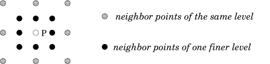
Figure 2: Description of the adjacent zone of a grid point $P$.

Note that the concept of adjacent zone is reasonable only for continuously propagating waves, as in case of our guided-wave applications, where in each time step the propagating waves do not travel far from the current position due to their finite propagation speed.

3.4 Reconstruction check

In this work we use the wavelet decompositions of the fields only to determine the adaptive grid. We do not propagate fields in their wavelet representations (cf. the statement in the first paragraph of Sec. 4). Thus at each time step, after adapting the grid using the FWT, and adding the adjacent zone, we need to restore the fields in the physical space by performing the inverse wavelet transformation (IWT). To this end, we may need to augment the adaptive grid with additional neighboring points (e.g. see Fig 3). This process of adding neighboring points needed to calculate the wavelet coefficients in the next time step is called reconstruction check. Fig 3 shows various possible scenarios, and the corresponding minimal set of the grid points required for calculation of the wavelet coefficients. The values of the wavelet coefficients at these newly added points are set to zero.

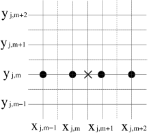
(a) $\times$: The point corresponding to $d^{1}_{j,m,n}$;  $\bullet$: The neighboring points needed to calculate $d^{1}_{j,m,n}$.

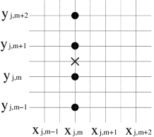
(b) $\times$: The point corresponding to $d^{2}_{j,m,n}$;  $\bullet$: The neighboring points needed to calculate $d^{2}_{j,m,n}$.

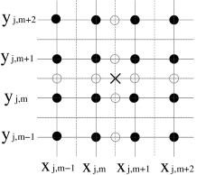
(c) $\times$: The point corresponding to $d^{3}_{j,m,n}$;  $\bullet$, $\circ$: The neighboring points needed to calculate $d^{3}_{j,m,n}$.

Figure 3: Descriptions of the neighboring points needed to calculate the wavelet coefficients $d^{\nu}_{j,m,n}$ with the orders $N=\tilde{N}=2$.

The efficiency of the wavelet transform depends on the number of the finest grid points only at the beginning; however, after the first compression, it depends solely on the cardinality (= number of grid points) of the adaptive grid.

3.5 Calculation of the spatial derivatives on the adaptive grid

After the adjacent zone correction and the reconstruction check, we are in a position to calculate the derivative of $f_{\zeta}$ at a grid point in the adaptive grid. For this we need to know the density level of this point, which is defined as the maximum of the $x$-level and the $z$-level of that point.

We illustrate this concept explicitly only for the $x$-level, the $z$-level can be determined analogously. For a point $Q=(x_{0},z_{0})$ in the adaptive grid $\mathcal{G}$, let $Q^{\prime}=(x_{1},z_{0})\in\mathcal{G}$ be the nearest point to $Q$. Then the $x$-level $Levelx$ of $Q$ relative to $\mathcal{G}$ is

$$Levelx:=j_{\max}-\log_{2}(\mathrm{dist}(Q,Q^{\prime})/\Delta x)$$ (9)

where $\Delta x$ is the smallest computational mesh size along the $x$ axis, and $\mathrm{dist}(Q,Q^{\prime})=|x_{1}-x_{0}|$. For $\mathrm{dist}(Q,Q^{\prime})=\Delta x$, the level $Levelx$ of $Q$ attains its maximum $j_{\max}$. For $\mathrm{dist}(Q,Q^{\prime})=2\Delta x$, we have $Levelx=j_{\max}-1$, etc. See Fig. 4 for an example of describing the density level of a grid point.

Figure 4: Description of the density level of a point $Q$ in an adaptive grid: the $x$-level of $Q$ is $j_{\max}-1$ and the $z$-level of $Q$ is $j_{\max}$, thus, the density level of $Q$ is $j_{\max}$.

Now we continue to discuss the derivative calculations. Suppose $j_{0}$ to be the density level of $Q$ in $\mathcal{G}$. Then, we can represent $f_{\zeta}$ by a finite sum ${\bf P}_{j_{0}}f$ locally in some neighborhood $\Omega_{0}$ of $Q$.

$${\bf P}_{j_{0}}f(x,z)=\sum_{m,n}\alpha_{j_{0},m,n}({\displaystyle\boldsymbol{\phi}}_{N})_{j_{0},m,n}(x,z),\quad(x,z)\in\Omega_{0}$$ (10)

We differentiate ${\bf P}_{j_{0}}f$ with respect to $x$ to approximate the $x$-derivative of $f$ at $Q$. If any points in the sum (10) are not present in $\mathcal{G}$, then we interpolate the values at these points by the IWT using the values of the coarser levels. From the interpolation property of $({\displaystyle\boldsymbol{\phi}}_{N})_{j_{0},m,n}$ we know that

$$\alpha_{j_{0},m,n}=2^{-j_{0}}({\bf P}_{j_{0}}f)\Big{(}\frac{m}{2^{j_{0}}},\frac{n}{2^{j_{0}}}\Big{)},\quad\text{for }m,n\in\mathbb{Z}.$$

Thus, we have

$$({\bf P}_{j_{0}}f)(x,z)=\sum_{m,n}({\bf P}_{j_{0}}f)\Big{(}\frac{m}{2^{j_{0}}},\frac{n}{2^{j_{0}}}\Big{)}\displaystyle DD_{N}\big{(}2^{j_{0}}x-m\big{)}\displaystyle DD_{N}\big{(}2^{j_{0}}z-n\big{)},\quad(x,z)\in\Omega_{0}.$$ (11)

Differentiate both sides of (11) with respect to $x$ gives

$$\frac{\partial({\bf P}_{j_{0}}f)}{\partial x}(x,z)=\sum_{m,n}({\bf P}_{j_{0}}f)\Big{(}\frac{m}{2^{j_{0}}},\frac{n}{2^{j_{0}}}\Big{)}\frac{\mathrm{d}\displaystyle DD_{N}\big{(}2^{j_{0}}x-m\big{)}}{\mathrm{d}x}\displaystyle DD_{N}\big{(}2^{j_{0}}z-n\big{)},\quad(x,z)\in\Omega_{0}.$$ (12)

The derivatives of $\displaystyle DD_{N}^{\prime}$ can be calculated exactly at the integers using the difference filters shown in Table 1 (see Ref. [16] for details of the derivation).

$i$	$N=2$	$N=3$	$N=4$
$1$	$2/3$	$272/365$	$39296/49553$
$2$	$-1/12$	$-53/365$	$-76113/396424$
$3$		$16/1095$	$1664/49553$
$4$		$1/2920$	$-2645/1189272$
$5$			$-128/743295$
$6$			$1/1189272$

Table 1: Difference filters $\{\displaystyle DD_{N}^{\prime}(i)\}_{i\in\mathbb{Z}}$ with consistency order $2N$. Note that $\displaystyle DD_{N}^{\prime}(i)=-\displaystyle DD_{N}^{\prime}(-i)$.

Since the density level of $Q$ is $j_{0}$, there exist $m^{\prime},n^{\prime}\in\mathbb{Z}$ such that $Q=\big{(}\frac{m^{\prime}}{2^{j_{0}}},\frac{n^{\prime}}{2^{j_{0}}}\big{)}$ and it is easy to see that

$$\frac{\partial({\bf P}_{j_{0}}f)}{\partial x}\Big{(}\frac{m^{\prime}}{2^{j_{0}}},\frac{n^{\prime}}{2^{j_{0}}}\Big{)} =\sum_{m,n}({\bf P}_{j_{0}}f)\Big{(}\frac{m}{2^{j_{0}}},\frac{n}{2^{j_{0}}}\Big{)}\frac{\mathrm{d}\displaystyle DD_{N}\big{(}m^{\prime}-m\big{)}}{\mathrm{d}x}\displaystyle DD_{N}\big{(}n^{\prime}-n\big{)}$$

$$=2^{j_{0}}\sum_{m}({\bf P}_{j_{0}}f)\Big{(}\frac{m}{2^{j_{0}}},\frac{n^{\prime}}{2^{j_{0}}}\Big{)}\displaystyle DD_{N}^{\prime}\big{(}m^{\prime}-m\big{)}.$$ (13)

Similarly,

$$\frac{\partial({\bf P}_{j_{0}}f)}{\partial z}\Big{(}\frac{m^{\prime}}{2^{j_{0}}},\frac{n^{\prime}}{2^{j_{0}}}\Big{)}=2^{j_{0}}\sum_{n}({\bf P}_{j_{0}}f)\Big{(}\frac{m^{\prime}}{2^{j_{0}}},\frac{n}{2^{j_{0}}}\Big{)}\displaystyle DD_{N}^{\prime}\big{(}n^{\prime}-n\big{)}.$$ (14)

This finishes the general discussion about the adaptive wavelet collocation method; in the next section, we apply it to Maxwell’s equations.

4 AWC-TD method for Maxwell’s equations

In this section we formulate the update scheme for Maxwell’s equations, and then elaborate on algorithmic issues related with the AWC-TD method. In the present formulation we represent the electric and magnetic fields in the physical space, and not in the wavelet space. To unleash the full power of adaptivity, however, the field representation and the update in wavelet space are advantageous.

We illustrate the method for the transverse magnetic (TM)_y setting given by (3). Similar procedure can also be formulated for TE_y setting in (2). Unlike the standard FDTD method, here the electric field and the magnetic field components are evaluated on same spatial grid, and their spatial derivatives are approximated at the same grid point. But the electric field components are sampled at integer time-steps, whereas the magnetic field components are sampled at half-integer time-steps.

4.1 Update scheme for the spatial derivative

For a point $Q$ in the adapted grid $\mathcal{G}$, let $\mathcal{H}_{x}|^{k+1/2}_{Q}$, $\mathcal{H}_{z}|^{k+1/2}_{Q}$ and $\mathcal{E}_{y}|^{k}_{Q}$ denote the discretized value of $\mathcal{H}_{x}$, $\mathcal{H}_{z}$ and $\mathcal{E}_{y}$ at the point $Q$, and at a time $(k+1/2)\Delta t$ for the magnetic field components and at a time $k\Delta t$ for the electric field component where $\Delta t>0$ is the time step size (Note that, the electric field components are sampled at integer time-steps, whereas the magnetic field components are sampled at half-integer time-steps.). Assume $j(Q)$ to be the density level of $Q$ relative to $\mathcal{G}$. Then we can represent the point $Q$ as $(x_{j(Q),m^{\prime}},z_{j(Q),n^{\prime}})$ for some $m^{\prime},n^{\prime}\in\mathbb{Z}$.

Let $L$ be the length of the computational domain $\Omega$. We rescale the wavelet decomposition (11) with the factor $L$. Then using the central difference scheme for the time derivatives and using (13)-(14) for the spatial derivatives, we get the following difference equations

$$\mathcal{H}_{x}|^{k+\frac{1}{2}}_{Q} =\mathcal{H}_{x}|^{k-\frac{1}{2}}_{Q}+\frac{\Delta t}{\mu_{0}}\frac{2^{j(Q)}}{L}\sum_{n}\mathcal{E}_{y}|^{k}_{(x_{j(Q),m^{\prime}},z_{j(Q),n})}\displaystyle DD_{N}^{\prime}(n^{\prime}-n),$$ (15a)

$$\mathcal{H}_{z}|^{k+\frac{1}{2}}_{Q} =\mathcal{H}_{z}|^{k-\frac{1}{2}}_{Q}+\frac{\Delta t}{\mu_{0}}\frac{2^{j(Q)}}{L}\sum_{m}\mathcal{E}_{y}|^{k}_{(x_{j(Q),m},z_{j(Q),n^{\prime}})}\displaystyle DD_{N}^{\prime}(m^{\prime}-m),$$ (15b)

$$\mathcal{E}_{y}|^{k+1}_{Q} =\mathcal{E}_{y}|^{k-1}_{Q}+\frac{\Delta t}{\varepsilon_{0}}\frac{1}{\varepsilon_{r}|_{Q}}\frac{2^{j(Q)}}{L}\Big{(}\sum_{n}\mathcal{H}_{x}|^{k+\frac{1}{2}}_{(x_{j(Q),m^{\prime}},z_{j(Q),n})}\displaystyle DD_{N}^{\prime}(n^{\prime}-n)$$

$$-\sum_{m}\mathcal{H}_{z}|^{k+\frac{1}{2}}_{(x_{j(Q),m},z_{j(Q),n^{\prime}})}\displaystyle DD_{N}^{\prime}(m^{\prime}-m)\Big{)},$$ (15c)

The first time step ($k=0$) is an explicit Euler step with step size $\Delta t/2$ using initial conditions for the fields at the time $t=0$. If not explicitly mentioned, otherwise the fields are set zero at the beginning for all our numerical experiments in Sec.  5. The update equations for the PML assisted Maxwell’s equations can be found in Ref. [9].

From the form of these update equations, it is clear that the AWC-TD method can be thought as an variant of high order FDTD method. The AWC-TD method is defined with respect to a locally adapted mesh, and unlike the FDTD method, it does not require a static (fixed), structured mesh. This will lead to efficient use of the computational resources. In the next section, we elaborate on algorithmic aspects of the method.

4.2 Update scheme for the time derivative

Several choices are available for time stepping. As in case of the standard FDTD method, we use in (15) the central difference scheme for the discretization of the time derivatives. For this explicit scheme, the smallest spatial step-size restricts the maximal time-step according to the Courant–Friedrichs–Lewy (CFL) stability condition. Using a uniform spatial mesh in the update equations (15) with a mesh size $\Delta$ in both coordinate directions the CFL condition reads

$$\Delta t\leq\frac{\Delta}{\sqrt{2}\mathrm{c}\sum_{l=0}^{l_{0}-1}|\displaystyle DD_{N}^{\prime}(l)|},$$ (16)

see [9, Sec. 3.5] and [22], where $\mathrm{c}$ is the speed of light in vacuum and $\{\displaystyle DD_{N}^{\prime}(l)\}$ is the known derivative filter of the ISF as in Table 1. Due to the local adaptive grid strategy of the AWC-TD method, we cannot define a global stability criteria as above. But choosing $\Delta$ to be the smallest step size in the adaptive grid, we get a conservative bound for $\Delta t$ via (16) for the AWC-TD method. In the simulation tests (in this paper, and in [9]) we did not experience any stability related issues with this modus operandi.

4.3 Implementation aspects

4.3.1 Grid management

In AWC method the computational grid is changed with the state (spatial localization) of the propagating field. Thus the grid management is one of the important steps in the implementation of this method. This is done as following: We store the information of the adaptive grid into a 2D Boolean array called a grid mask or simply a mask, whose size is square the number of the finest grid points along one direction. We use 2D arrays of real numbers with the size of the grid mask to store the fields such as $\mathcal{E}_{y}$, $\mathcal{H}_{x}$, and $\mathcal{H}_{z}$ etc. Note that the computational effort for updating the fields at each time step is proportional to the cardinality (i.e. the number of entries in the mask with value $1$) of the adaptive grid.

If the value of an entry of a mask is $true$ or $1$, then the corresponding grid point is included in the adaptive grid; otherwise, it is not included in the grid. Thus by forcing the value of an entry of a mask to $1$, we can include the corresponding point to the grid, or by forcing the entry to $0$, we can exclude the corresponding point from the grid.

4.3.2 Algorithmic procedures

Algorithm 1 outlines the main function awcm_main() of AWC-TD method for TM_y setting. It mainly consists of two blocks of operations: The first block is initialization, and the second block is time stepping. In the time stepping block, at each time step the routines awcm_adaptive() and awcm_update() are called. The former routine optimally adapts the computational grid for the field updates at the next time step, whereas the latter routine calculates the spatial derivatives on the non-equidistant, adaptive grid, and updates the field values.

# Initialization

awcm_initialize()

# ———————————————————————————————————–

# Time stepping of $\mathcal{E}_{y}$, $\mathcal{H}_{x}$ and $\mathcal{H}_{z}$

for $t\leq T$ do

       # Adapt the grid for $t+\Delta t$ according to $\mathcal{E}_{y}^{t}$, see Algorithm 2.

       awcm_adaptive()

       # ——————————————————————————————————

       # Update $\mathcal{H}_{x}^{t+\Delta t/2}$, $\mathcal{H}_{z}^{t+\Delta t/2}$ and $\mathcal{E}_{y}^{t+\Delta t}$, see Algorithm 3.

       awcm_update()

      

       # ——————————————————————————————————

       # Go to the next time step.

       $t=t+\Delta t$

Algorithm 1 awcm_main() for TM_y settings

The initialization subroutine awcm_initialize() ensures that various required inputs for the AWC method are systematically prepared. It consists of checking the given initial data (i.e. for time step $k=0$) ${\mathcal{H}_{x}}^{-\frac{1}{2}}$, ${\mathcal{H}_{z}}^{-\frac{1}{2}}$ and ${\mathcal{E}_{y}}^{0}$ at the finest resolution level $j_{max}$, the threshold $\zeta$, the maximum and the minimum spatial resolution levels $j_{max}$ and $j_{min}$ respectively, and the number of time steps $k_{max}$. The time step $\Delta t$ is chosen such that it satisfies the CFL condition given by (16).

The adaptivity procedure in Algorithm 1 handled by a subroutine awcm_adaptive() is outlined in Algorithm 2. It is done by means of a 2D array $\mathcal{E}_{y}$ with a mask $Mask0$. For later use, we store a copy of $Mask0$ in $pMask0$, since $Mask0$ will be modified by the subsequent subroutines. The duplicate $pMask0$ serves as a reference for finding those points which need to be interpolated before we can update the fields. We perform the fast wavelet transform of $\mathcal{E}_{y}$ on $Mask0$. Note that $Mask0$ is either fully $1$ (as at the beginning) or a reconstruction check has been performed in the previous time step. In any case, FWTs on $Mask0$ are always possible. By the FWT applied to $\mathcal{E}_{y}$ we obtain the scaling coefficients on the coarsest level $j_{\min}$, and the wavelet coefficients on levels from $j_{\min}$ to $j_{\max}-1$.

For each wavelet coefficient, we compare its absolute value with the given tolerance $\zeta$. If it is less than $\zeta$, we remove the corresponding point from $Mask0$. Next, we determine the adjacent zone for each point in $Mask0$, and then modify $Mask0$ to include all points in these adjacent zones. Finally, a reconstruction check is applied to $Mask0$ so that the FWT in the next time step is well defined. The latter two processes are done in the subroutine Maskext($Mask0$) as shown in Algorithm 2.

# Store $Mask0$ into $pMask0$.

# $pMask0$: The adaptive grid for $\mathcal{E}_{y}$ at current time step.

$pMask0=Mask0$

# ————————————————————————————————————

# Fast wavelet transform of $\mathcal{E}_{y}$ on $Mask0$ with $\zeta$.

# $\mathcal{E}_{y}$ is converted into coefficients of wavelet domain, $Mask0$ is thinned.

FWT($\mathcal{E}_{y}$, $Mask0$, $\zeta$)

# ————————————————————————————————————

# Add adjacent zone and perform a reconstruction check to $Mask0$.

Maskext($Mask0$)

# ————————————————————————————————————

# Add points needed to calculate $\frac{\partial\mathcal{E}_{y}}{\partial x}$ and $\frac{\partial\mathcal{E}_{y}}{\partial z}$ on $Mask0$.

# 1. Determine the density level of each point in $Mask0$.

$Level0=$ Level($Mask0$)

# 2. Initialize $Mask1$ with $Mask0$.

$Mask1=Mask0$

# 3. Update $Mask1$.

gMaskext($Mask1$, $Level0$)

# ————————————————————————————————————

# Add points needed to calculate $\frac{\partial\mathcal{H}_{x}}{\partial z}$ and $\frac{\partial\mathcal{H}_{z}}{\partial x}$ on $Mask1$.

# 1. Determine the density level of each point in $Mask1$.

$Level1=$ Level($Mask1$)

# 2. Initialize $Mask2$ with $Mask1$.

$Mask2=Mask1$

# 3. Update $Mask2$.

gMaskext($Mask2$, $Level1$)

# ————————————————————————————————————

# Inverse wavelet transform of the values $\mathcal{E}_{y}$ in the wavelet domain on $Mask2$.

# $\mathcal{E}_{y}$ is reconstructed from the values in the wavelet domain on $Mask2$.

IWT($\mathcal{E}_{y}$, $Mask2$)

Algorithm 2 awcm_adaptive() for TM_y settings

After the above adaptation of the grid is done, we still need to make further reconstructions on this grid, so that it will allow computation of the field derivatives required for the field update. For updating $\mathcal{H}_{x}$ and $\mathcal{H}_{z}$, we need $\frac{\partial\mathcal{E}_{y}}{\partial z}$ and $\frac{\partial\mathcal{E}_{y}}{\partial x}$ (see (3) or (15)). To calculate these spatial derivatives of the electric field, we interpolate values of $\mathcal{E}_{y}$ at those neighbors of points in $Mask0$ which are not already in $Mask0$. We store the information of $Mask0$ into $Mask1$. Further, we add all points to $Mask1$ needed in the calculations of spatial derivatives according to the density levels of the points in $Mask1$. These density levels are computed in subroutine Level($Mask1$) and stored in the 2D array $Level0$. Again a reconstruction check of $Mask1$ is required to enable IWTs. This is done by the subroutine gMaskext($Mask1$, $Level0$).

Then we need to follow the same procedure as above for updating $\mathcal{E}_{y}$ using the spatial derivatives $\frac{\partial\mathcal{H}_{x}}{\partial z}$ and $\frac{\partial\mathcal{H}_{z}}{\partial x}$. Again we add the neighboring points needed for calculations of the spatial derivatives of the magnetic field. We copy $Mask1$ to $Mask2$, and calculate the density level array $Level1$ of $Mask2$. The necessary reconstruction check is then done by calling gMaskext($Mask2$,$Level1$). The call of IWT($\mathcal{E}_{y}$, $Mask2$) to reconstruct $\mathcal{E}_{y}$ in the physical domain finishes the routine awcm_adaptive() in Algorithm 2.

Next, we update the field values on the adaptive grid, which is described by Algorithms 3. Since the adaptive grid may change with time, we need to interpolate the field values at points in the adaptive grid of the current time step, which are not included in the adaptive grid of the previous time step. For example, consider the update of $\mathcal{H}_{x}$ about a grid point $Q$ at a time $(k+1/2)\Delta t$ in (15a). Since $Q$ is not necessarily in the adaptive grid of previous time $(k-1/2)\Delta t$, the value $\mathcal{H}_{x}|_{Q}^{k-1/2}$ in (15a) must be interpolated. Once this is done, Algorithm 4 calculates the spatial derivatives of each field components on the adaptive grid, and then the fields are updated.

# To update $\mathcal{H}_{x}$:

# Interpolate $\mathcal{H}_{x}$ on points in $Mask1$ which are not in $pMask0$ using inverse wavelet transform.

interpolate($\mathcal{H}_{x}$, $pMask0$, $Mask1$)

# Calculate $\frac{\partial\mathcal{E}_{y}}{\partial z}$ on $Mask1$ using Algorithm 4.

$dA_{z}=$ diffz($\mathcal{E}_{y}$, $Mask1$, $Level1$, dfilter, $dz$)

Update $\mathcal{H}_{x}$ on $Mask1$ using $dA_{z}$ as per formulation in (15a).

# ————————————————————————————————————

# To update $\mathcal{H}_{z}$:

# Interpolate $\mathcal{H}_{z}$ on points in $Mask1$ which are not in $pMask0$ using inverse wavelet transform.

interpolate($\mathcal{H}_{z}$, $pMask0$, $Mask1$)

# Calculate $\frac{\partial\mathcal{E}_{y}}{\partial x}$ on $Mask1$ using Algorithm 4.

$dA_{x}=$ diffx($\mathcal{E}_{y}$, $Mask1$, $Level1$, dfilter, $dx$)

Update $\mathcal{H}_{z}$ on $Mask1$ using $dA_{x}$ as per formulation in (15b).

# ————————————————————————————————————

# To update $\mathcal{E}_{y}$:

# Interpolate $\mathcal{E}_{y}$ on points in $Mask0$ which are not in $pMask0$ using inverse wavelet transform.

interpolate($\mathcal{E}_{y}$, $pMask0$, $Mask0$)

# Calculate $\frac{\partial\mathcal{H}_{x}}{\partial z}$ and $\frac{\partial\mathcal{H}_{z}}{\partial x}$ on $Mask0$, see the Algorithm 4.

# diffx() is defined in Algorithm 4. diffz() is similarly defined.

$dA_{z}=$ diffz($\mathcal{H}_{x}$, $Mask0$, $Level0$, dfilter, $dz$)

$dA_{x}=$ diffx($\mathcal{H}_{z}$, $Mask0$, $Level0$, dfilter, $dx$)

Update $\mathcal{E}_{y}$ on $Mask0$ using $dA_{z}$ and $dA_{x}$ as per formulation in (15c).

Algorithm 3 awcm_update() for TM_y settings

Input : $A$ = 2D array of field values

$Mask$ = grid mask,

$Level$ = $x$-level of each point in $Mask$,

dfilter difference filters as given in Table 1,

$dx$ = the smallest mesh size in $x$ direction at the highest resolution level

Return : a 2D array of $\frac{\partial A}{\partial x}$ on $Mask$

# Initialize a 2D array $dA$ for the storage of $\frac{\partial A}{\partial x}$.

$dA=0$

$\mathcal{K}_{j}=\{(x_{j,m},y_{j,n})\,|\,m,n=0,1,\dots,2^{j}\}$, where $x_{j,m}=\dfrac{mL}{2^{j}},y_{j,n}=\dfrac{nL}{2^{j}}$, for $j_{\min}\leq j\leq j_{\max}$.

forall $Q=(x_{j_{\max},m},y_{j_{\max},n})\in\mathcal{K}_{j_{\max}}$ do

       if $Q\in Mask$ then

             # Read the density level of $Q$ from $Level$.

             $j(Q)=Level[n][m]$

             Calculate $dA$ at point $Q$ using dfilter and values of $A$ at neighbor points in the level $j(Q)$

             as described in (13).

      

Algorithm 4 diffx($A$, $Mask$, $Level$, dfilter, $dx$)

5 Numerical results: Gaussian pulse propagation

In this section we demonstrate the applicability of the AWC-TD method. The method has been implemented in C++, and the computations have been performed on $32$ GB RAM, Linux system with AMD Opteron processors.

As an example, we consider propagation of a spatial Gaussian pulse in free space ($\varepsilon_{r}=1$). We solve a system of TM_y equations within a square domain $\Omega=[-L/2,L/2]\times[-L/2,L/2]$ in the $XZ$ plane. We set the domain length $L=6.0$ $\mu$m, the PML width $d=L/4$, and the initial spatial Gaussian excitation $\mathcal{E}_{y}(x,z,0)=\exp(-(x^{2}+z^{2})/(2\sigma^{2}))$ with the Gaussian pulse width $\sigma=1/(4\,\sqrt{2})$ $\mu$m. Implementation details about the PML can be found in Ref. [9].

Our minimum and maximum resolution levels are $j_{\min}=3$ and $j_{\max}=9$ inducing the smallest mesh size $\Delta=\Delta x=\Delta z=L/2^{j_{max}}=11.71875$ nm. The temporal error of the AWC-TD method is controlled by $O(\Delta t^{2})$ if we do not consider the compression, which is the consistency order of the central difference discretization of the time derivatives. Accordingly, a reasonable choice for the threshold $\zeta$ is a value slightly larger than the discretization error. As the orders of the underlying interpolating scaling function/wavelet pair is $N=\tilde{N}=4$, we set $\Delta t=\Delta/\mathrm{c}/1.6$, which is just below the maximal step size from the CFL condition (16). For this setting, a choice of wavelet threshold $\zeta=5.0\times 10^{-4}$ experimentally turned out to be sufficient concerning both adaptivity and accuracy.

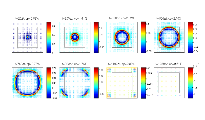
Figure 5: Evolution of the initial excitation $\mathcal{E}_{y}(x,z,0)=\exp(-(x^{2}+z^{2})/(2\sigma^{2}))$ in the $XZ$ plane with $\sigma=1/(4\,\sqrt{2})$ $\mu$m, $N=\tilde{N}=4$ and $\zeta=5.0\times 10^{-4}$. On top of each time frame, time and grid compression rate cp are given (cp is the ratio of the cardinality of the adaptive grid and the cardinality of the full grid with a uniform step size $\Delta$ (= the smallest mesh size) in the both coordinate directions). The adaptive grid systematically follows and resolves the wavefront. In regions where the field is small or not present only grid points of the coarsest level are assigned. For an animation movie, see the YouTube channel: www.youtube.com/user/HaojunLi#p/u/1/2Yzpjf7Xnp4.

The Gaussian pulse, launched in the center of the computational domain, spreads away from the center as time evolves. Fig. 5 illustrates how the adaptive grid systematically follows and resolves the wavefront. Since the electromagnetic field energy is spreading in all directions, the field’s amplitude is decreasing (unlike as in 1D, where during the propagation the amplitude stays at half of the initial value, see [9, Sec. 4.4.1]). The AWC method generates a detailed mesh only in the regions where the field is localized, the mesh gets coarse in other parts of the computational domain. As seen in the snapshots for $t=200\Delta t$ or $t=920\Delta t$, it is evident that depending on the extend of the field localization, the density of the grid points varies accordingly.

A figure of merit for the performance of the AWC-TD method is the compression rate cp, which is defined as a ratio of the cardinality of the adaptive grid and the cardinality of the full grid with a uniform step size $\Delta$ (= the smallest mesh size) in the both coordinate directions. The percentage cp on the top of each time frame in Fig. 5 shows the grid compression rate. Since the extent of a spatial localization of a pulse depends on its frequency contents, the compression rate cp for the test case in Fig. 5 varies (also seen in Fig. 7). Nevertheless, for all time steps the number of grid points in the adapted grid is substantially less than that of in the full grid; but still the AWC method resolves the pulse very well with an optimal (with respect to the given threshold $\zeta$) allocation of the grid points.

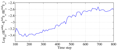
Figure 6: Relative Error in $\mathcal{E}_{y}$ between the adaptive wavelet collocation method and the full grid wavelet method.

The relative maximal error of $\mathcal{E}_{y}$ field values over $\Omega$ between the adaptive and the full grid methods as the time evolves is shown in Fig. 6. Despite of grid compression (which can be quite significant at some time instants, as seen in Fig. 5), the solution by the AWC method is quite close to that of by the full grid method. As mentioned earlier, as the pulse spreads in all the direction, the field becomes weak, and the real performance gain by the adaptivity effectively reduces. It is reflected in the apparent increase in the relative maximal error (with respect to the full grid method) in Fig. 6. Note that when the field has completely left the computational domain $\Omega$ roughly after $800$ time steps, the error over $\Omega$ is not defined meaningfully any more.

Fig. 7 demonstrates that (the major part of) the computational effort of the AWC-TD method per time step is indeed proportional to the cardinality of the adapted grid at that time instant. To this end, we recorded the CPU time for every ten time steps (Fig. 7 top). For comparison, we also plotted the grid compression rate as a function of the time step (Fig. 7 bottom). Both functions progress in parallel, thus validating the above assertion about the numerical effort of the AWC-TD method.

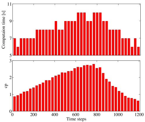
Figure 7: CPU time (top) and grid compression rate cp (bottom) as functions of the time step. Both functions progress in parallel which illustrates the fact that the numerical effort of the AWC-TD method for each time step is proportional to the number of points in the actual grid.

6 Conclusions

In this paper we investigated an adaptive wavelet collocation time domain method for the numerical solution of Maxwell’s equations. In this method a computational grid is dynamically adapted at each time step by using the wavelet decomposition of the field at that time instant. With additional amendments (e.g. adjacent zone corrections, reconstruction check, etc.) to the adapted grid, we formulated explicit time stepping update scheme for the field evolution, which is a variant of high order FDTD method, and is defined with respect to the locally adapted mesh. We illustrated that the AWC-TD method has high compression rate. Since (the major part of) the computational cost of the method per time step is proportional to the cardinality of the adapted grid at that time instant, it allows efficient use of computational resources.

This method is especially suitable for simulation of guided-wave phenomena as in the case of integrated optics devices. Initial studies for simulation of integrated optics microring resonators can be found in [9]. In the present feasibility study we represented the electric and magnetic fields in the physical space, and not in the wavelet space. To unleash the full power of adaptivity, however, the field representation and the update in wavelet space are mandatory.

References

- [1] K. Okamoto, Fundamentals of Optical Waveguides, Academic Press, U.S.A, 2000.
- [2] A. Taflove, S. C. Hagness, Computational Electrodynamics: The Finite-Difference Time-Domain Method, 3rd Edition, Artech House, 2005.
- [3] J. Hesthaven, T. Warburton, Nodal Discontinuous Galerkin Methods: Algorithms, Analysis, and Applications, Springer Texts in Applied Mathematics, Springer Verlag, 2008.
- [4] M. Fujii, W. J. R. Hoefer, Wavelet formulation of the finite-difference method: Full-vector analysis of optical waveguide junctions, IEEE J. Quantum Electron. 37 (8) (2001) 1015–1029.
- [5] O. V. Vasilyev, C. Bowman, Second-generation wavelet collocation method for the solution of partial differential equations, J. Comput. Phys. 165 (2000) 660–693.
- [6] O. V. Vasilyev, Solving multi-dimensional evolution problems with localized structures using second generation wavelets, Int. J. Comput. Fluid Dynamics 17 (2) (2003) 151–168.
- [7] J. Berenger, A perfectly matched layer for the absorption of electromagnetic waves, J. Comput. Phys. 114 (1994) 185–200.
- [8] S. D. Gedney, An anisotropic perfectly matched layer-absorbing medium for the truncation of FDTD lattices, IEEE Trans. Antennas Propagation 44 (12) (1996) 1630–1639.
- [9] H. Li, Numerical simulation of a micro-ring resonator with adaptive wavelet collocation method, Ph.D. thesis, Karlsruhe Institute of Technology, Germany, online available from http://digbib.ubka.uni-karlsruhe.de/volltexte/1000024186 (July 2011).
- [10] S. Mallat, Multiresolution approximations and wavelet orthonormal bases of , Trans. Amer. Math. Soc. 315 (1989) 69–87.
- [11] S. Mallat, A Wavelet Tour of Signal Processing, 2nd Edition, Academic Press, 1998.
- [12] O. V. Vasilyev, S. Paolucci, A dynamically adaptive multilevel wavelet collocation method for solving partial differential equations in a finite domain, J. Comput. Phys. 125 (1996) 498–512.
- [13] O. V. Vasilyev, S. Paolucci, A fast adaptive wavelet collocation algorithm for multidimensional PDEs, J. Comput. Phys. 138 (1997) 16–56.
- [14] I. Daubechies, Ten Lectures on Wavelets, CBMS-NSF Regional Conf. Series in Appl. Math. 61, SIAM, 1992.
- [15] A. K. Louis, P. Maass, A. Rieder, Wavelets. Theory and Applications, Pure and Applied Mathemetics, Wiley, Chichester, 1997.
- [16] G. Deslauriers, S. Dubuc, Symmetric iterative interpolation processes, Constr. Approx. 5 (1989) 49–68.
- [17] W. Sweldens, The lifting scheme: A custom-design construction of biorthogonal wavelets, Appl. Comput. Harmon. Anal. 3 (1996) 186–200.
- [18] W. Sweldens, The lifting scheme: A consctruction of second generation wavelets, SIAM, J. Math. Anal 29 (2) (1998) 511–546.
- [19] S. Dubuc, Interpolation through an iterative scheme, J. Math. Anal. Appl 114 (1986) 185–204.
- [20] D. L. Donoho, Interpolating wavelet transforms, Tech. rep., Department of Statistics, Stanford University (1992).
- [21] S. Goedecker, Wavelets and their applications for the solution of partial differential equations in physics, Vol. 4, Presses Polytechniques et Universitaires Romandes, 1998.
- [22] E. M. Tentzeris, R. L. Robertson, J. F. Harvey, L. P. B. Katehi, Stability and dispersion analysis of Battle-Lemarie-based MRTD schemes, IEEE Trans. Microwave Theory and Techniques 47 (7) (1999) 1004–1013.