The stellar metallicity distribution of disc galaxies and bulges in cosmological simulations

Abstract

By means of high-resolution cosmological hydrodynamical simulations of Milky Way-like disc galaxies, we conduct an analysis of the associated stellar metallicity distribution functions (MDFs). After undertaking a kinematic decomposition of each simulation into spheroid and disc sub-components, we compare the predicted MDFs to those observed in the solar neighbourhood and the Galactic bulge. The effects of the star formation density threshold are visible in the star formation histories, which show a modulation in their behaviour driven by the threshold. The derived MDFs show median metallicities lower by 0.2$-$0.3 dex than the MDF observed locally in the disc and in the Galactic bulge. Possible reasons for this apparent discrepancy include the use of low stellar yields and/or centrally-concentrated star formation. The dispersions are larger than the one of the observed MDF; this could be due to simulated discs being kinematically hotter relative to the Milky Way. The fraction of low metallicity stars is largely overestimated, visible from the more negatively skewed MDF with respect to the observational sample. For our fiducial Milky Way analog, we study the metallicity distribution of the stars born in situ relative to those formed via accretion (from disrupted satellites), and demonstrate that this low-metallicity tail to the MDF is populated primarily by accreted stars. Enhanced supernova and stellar radiation energy feedback to the surrounding interstellar media of these pre-disrupted satellites is suggested as an important regulator of the MDF skewness.

1 Introduction

Galaxy formation and evolution is a distinctly multi-disciplinary field, connecting fundamental cosmology and structure formation, through stellar astrophysics, nucleosynthesis, and therefore atomic physics. These extremes manifest themselves in the appearance and characteristics of the stellar populations which comprise the galaxies we observe empirically.

Because of the obvious, deep-rooted, interest in understanding the origin of our own Milky Way, there are intense efforts underway to understand the underlying physics driving disc galaxy formation within the concordant $\Lambda$CDM cosmology. From an empirical perspective, the Milky Way clearly possesses the greatest wealth of observational constraints to any formation scenario, from accurate 6d phase-space coordinates (positions and velocities), chemical abundances, and ages, for massive numbers of halo, disc, and bulge stars (e.g., Freeman & Bland-Hawthorn 2002).

Galactic chemical evolution models developed in a cosmological framework are particularly fruitful tools to derive crucial information regarding the star formation histories (SFH) of galaxies, on the ages of the stellar populations, and on the gas accretion and outflow histories. A key observable for constraining any such model is the metallicity distribution function (MDF) of the stars of the various sub-components of a galaxy. The MDF bears information concerning the star formation history of our Galaxy (e.g. Tinsley 1980; Matteucci & Brocato 1990; Pagel & Tautvaisiene 1995; Caimmi 1997; Haywood 2006), which is directly linked to the merging history of its progenitors, i.e. the “building blocks” of the various components. A detailed study of the impact of the accretion history on the shape of the MDF can be found in Font et al. (2006), where it was shown that the earlier the major accretion epoch of satellites of the central galaxy, the more the MDF peak is shifted toward lower metallicities. These works show how the study of the MDF is important to gain information on the evolution of both the dark matter content of these systems and of the baryonic matter, governed by various physical processes which lead ultimately to self-regulated star formation. The metal content of galaxies grows with time (modulo dilution effects from metal-poor infall and metal-rich outflows), hence the disc MDF allows us to track the enrichment history of the Milky Way empirically and the enrichment history of simulated Milky Way-like analogs disc through model ‘deconstruction’. The extreme, metal-poor tail of the MDF provides crucial information on the earliest enrichment phases of the disc, while the most metal-rich stars bear the imprint of the latest galactic evolutionary stages.

In what follows, we study the MDFs of the discs and bulges associated with a family of high-resolution cosmological hydrodynamical simulations. These tools represent an ideal instrument to follow the dynamical and chemical evolution of the Galactic stellar populations from first principles, with a detailed knowledge at any timestep of the spatial distibution of gaseous and stellar matter. This facilitates comparison with observational data, in particular local solar neighbourhood stars, since in the simulations, the position of each stellar particle is known and it is hence straightforward to select physical regions whose properties can be associated to those observed in the solar neighbourhood. The specific simulations employed in our analysis are described in §2, the results presented in §3, and our conclusions drawn in §4.

2 Model Description

The six simulations employed here are drawn from the MUGS sample (Stinson et al. 2010). From these, we derive the MDFs associated with their analogous ‘solar neighbourhoods’ and ‘bulges’, and contrast them with those measured in the Milky Way. Below, we provide an overview of the six simulations, along with the kinematic decomposition employed to separate disc stars from spheroid stars. A more extensive background to the simulations is provided by Stinson et al. (2010), while the radial and vertical metallicity gradients are explored by Pilkington et al. (2012a).

2.1 The MUGS Simulations

The MUGS simulations were run using the gravitational N-body $+$ SPH code Gasoline (Wadsley et al. 2004). Here, we provide a brief overview of the star formation and feedback recipes employed, as they impact most directly on the chemical abundances associated with the stellar populations; full details of the simulation are given in Stinson et al. (2010). The basic star formation and supernova feedback follows the ‘blastwave scenario’ of Stinson et al. (2006); stars can form from SPH gas particles which meet specific density ($>$1 cm^-3), temperature ($<$15000 K) and convergent flow criteria. When these are met, stars can form with a star formation rate $dM_{\star}/dt$ given by

$$\frac{dM_{\star}}{dt}=c^{\star}\frac{M_{gas}}{t_{dyn}},$$ (1)

where c${}^{\star}=0.015$ represents the star formation efficiency. This quantity is tuned in order to match the Kennicutt law for star formation in local disc galaxies (Kennicutt 1998). The quantity $M_{gas}$ is the mass of the star-forming gas particle, while $t_{dyn}$ is its dynamical timescale.

Within each ‘star’ particle, ‘individual’ star masses are distributed according to a Kroupa, Tout & Gilmore (1993) initial mass function (IMF), with lower and upper mass limits of 0.1 M_⊙ and 100 M_⊙, respectively. Stars with masses between 8 M_⊙ and 40 M_⊙ are assumed to explode as Type II supernovae (SNeII). Each supernova is assumed to possess an energy of 10⁵¹ erg, and we assume 40% of this energy is made available in the form of thermal energy to the surrounding interstellar medium (ISM).

The heavy elements restored to the ISM by SNeII in this version of Gasoline are O and Fe. Analytical power-law fits in mass were made using the yields of Woosley & Weaver (1995), convolved with the aforementioned Kroupa et al. (1993) IMF, to derive the mass fraction of metals ejected by SNeII for each stellar particle. These elements are returned on the timescale of the lifetimes of the individual stars comprising the IMF, after Raiteri et al. (1996). Type Ia supernovae (SNeIa) are included within Gasoline, patterned again after the Raiteri et al. implementation of the Greggio & Renzini (1983) single-degenerate progenitor model. Each SNeIa is assumed to return 0.63 M_⊙ of iron and 0.13 M_⊙ of oxygen to the ISM. This is an important feature of the code, which differentiates it from other previous attempts to model chemical abundances in simulations. In the past,cosmological codes tracked the total gas metallicity (Z), under the assumption of the instantaneous recycling approximation, i.e. neglecting the time delay between star formation and the energetic and chemical feedback from stellar winds and SNe (e. g., Sanchez-Blazquez et al. 2009). Such codes are not suited to study elements such as Fe, mainly produced by type Ia SNe on timescales varing from 0.03 Gyr up to several Gyr, but which are crucial since they are primary metallicity tracers, in particular in observational studies of the stellar MDF. In this paper, we take into account finite time delays for the main channels for Fe production, i.e. type Ia and type II SNe, hence our study should be regarded as a significant step forward with respect to previous studies of chemical abundances in cosmological simulations. Other recent chemical evolution studies in fully cosmological disc simulations relaxing the instantaneous recycling approximation include Rahimi et al. (2010) and Few et al. (2012).

The contribution of single low and intermediate mass asymptotic giant branch stars is not included in these runs, but for the analysis of oxygen and iron, this is negligible with respect to the contributions of SNeII and SNeIa.

The total metallicity in this version of Gasoline is tracked by assuming Z$\equiv$O+Fe. to this purpose, our next generation of runs with Gasoline will employ a more complete chemical ‘network’, ensuring that $\sim$90% of the global metallicity ‘Z’ will be tracked element-by-element (see Pilkington et al. 2012b). For these runs, only the solar metallicity yields were employed, and long-lived SNeIa progenitors (i.e. those in binary systems with companions having mass $m$$<$1.5 M_⊙) were neglected. For a Kroupa et al. (1993) IMF, in a simple stellar population the amount of Fe produced by the progenitors with mass $m$$<$1.5 M_⊙ is only $\sim$20% of the amount produced by all progenitors, i.e. with masses ranging from $0.8M_{\odot}$ to $8M_{\odot}$. While not important for our MDF work here, the systematic neglect of long-lived SNeIa progenitors could have a potential impact on the [O/Fe]-[Fe/H] relationship (Pilkington et al., in preparation).

For our analysis, we selected six galaxies with the most prominent discs, following the same criteria as described in Pilkington et al. (2012a). Each of the six MUGS simulations analysed here were run in a 50$h^{-1}$ Mpc cosmological box with ‘volume renormalization’ to ensure higher space and force resolution in the region centred on the central galaxy (Klypin et al. 2001). For each simulation, the $z$=0 output was examined to find sufficiently isolated halos within the mass range 5$\times$10¹¹ M_⊙ and 2$\times$10¹² M_⊙. Sixteen halos within this range were selected at random and re-run at higher resolution (9 of which are described by Stinson et al. 2010, with a further 7 now having been realised subsequent to the publication of the first sample). Six galaxies were chosen from the MUGS suite’: g1536, g24334, g28547, g422, g8893, and g15784. The system g15784 is our adopted fiducial Milky Way analog, owing to its total mass and its baryonic mass in the disc, both similar to the values calculated with up-to-date dynamical models of our Galaxy (see McMillan 2011).

In Table 1, we list the key properties for each of the simulations employed here. Following the same notation as the original MUGS simulations, galaxies are identified using the group number from the original friends-of-friends galaxy catalogue. The first column contains the galaxy name; the second, third, and fourth columns are, for each galaxy, the total (baryonic and non-baryonic) mass, the gas mass, and the stellar mass inside the virial radius $R_{vir}$, respectively. The fifth, sixth, and seventh columns are the corresponding number of dark matter particles, gas particles, and stellar particles, respectively. The eigth and ninth columns are the total disc mass and the total bulge mass assigned to each sub-component, after application of the kinematic decomposition and spatial cuts described in Sections 2.2 and 2.3. The final two columns are the half mass radius for the spheroid component ($R_{eff}$) and the disc scalelength ($R_{d}$), calculated by means of an exponential profile fit to the disc component.

2.2 Kinematic Decomposition

To isolate the stellar components associated with the simulated bulge and disc for each simulation, we performed kinematic decompositions, after Abadi et al. (2003). We first centre and align the angular momentum vectors of the baryons with the $z$-axis of the volume, and remove any systemic velocity associated with the simulated galaxy, for ease of subsequent decomposition.

We next compute the Lindblad Diagram of all stellar particles in the inner region of the halo ($r$$<$30 kpc), i.e. the $z$-component of the specific angular momentum as a function of the specific binding energy. An example is shown in Fig 1 (top left panel) for the fiducial simulation g15784. The distribution of the orbital circularity $\epsilon_{J}$ is then constructed, where $\epsilon_{J}=J_{z}/J_{circ}(E)$ where $J_{z}$ is the $z$-component of the specific angular momentum and $J_{circ}(E)$ the angular momentum of a circular orbit at a given specific binding energy. The $J_{circ}(E)$ curve (shown as a white line in the top-left panel of Fig. 1) indicates the location of circular orbits corotating with the disc.

The spheroid component (comprised of both bulge and inner halo stars) is defined a priori to be a symmetric distribution centered on $J_{z}/J_{circ}(E)=0$. This means that, by construction, the bulge/inner halo components are assumed to be non-rotating. Since we are here interested in distinguishing the bulge from the disc component, we assume that the disc is made by all the stars except those belonging to the bulge. Star particles with negative circularity are assigned to the spheroid component; those with positive circularity are randomly assigned to either the spheroid or disc components, weighted by the likelihood imposed by the relative numbers of both components at a given positive $J_{z}/J_{circ}(E)$. To prevent stars of nearby satellites from being included in our analysis, we perform a further spatial cut as described in  2.3.

This method, while somewhat arbitrary in its definition of the components, does allow one to decompose in an objective, ’hands-off’ manner, the stellar component into spheroidal and disc component, as shown graphically in the bottom panels of Fig. 1.

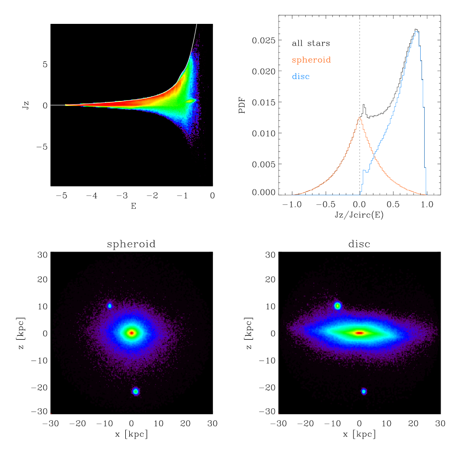
Figure 1: Kinematic decomposition of g15784. Top left panel: the $z$-component of the specific angular momentum shown as a function of specific binding energy for all stars within 30 kpc of the centre of the galaxy. The white curve shows the $J_{circ}(E)$ location. The colours scale with the density of particles in each pixel, with redder colours corresponding to higher densities. Top right panel: distribution of the orbital circularity of the stellar component (black line) and the decomposition into spheroid (orange line) and disc (blue line) components. Bottom panels: images of the spheroid (left) and disc (right) components. The colours scale with the density of particles in each pixel, with redder colours corresponding to higher densities. The sub-structure/peak near $J_{z}/J_{circ}(E)\sim+0.1$ is associated with the satellite seen at $(x,z)\sim(-10,+10)$ in the lower-right panel.

2.3 Spatial Cuts

In addition to the kinematic decomposition of Sect.2.2, for each galaxy we also applied a spatial cut to both the spheroid and disc components. Spheroid stars within $R_{b,cut}$=1$-$3 kpc are assigned to the ‘bulge’, a radial ‘cut’ which qualitatively corresponds to the spatial extent of the simulated bulge, although we have confirmed that the exact value selected within this range does not impact on our conclusions. Further, for each simulation, we assign stars to the disc should they lie within 4 kpc of the mid-plane, beyond the aforementioned bulge-disc radial cut, i.e. $r^{\prime}=\sqrt{X^{2}+Y^{2}}>R_{b,cut}$.

For one simulation (g24334), an additional spatial cut was applied, in order to remove the presence of a dwarf satellite which, at redshift $z$=0, is passing through the disk at $r^{\prime}$$\sim$5 kpc. The disc for g24334 was, instead, defined by $R_{b,cut}$$<$$r^{\prime}$$<$4 kpc.

Table 1: Main features of the simulated galaxies from the MUGS sample. All masses are expressed in units of $10^{10}M_{\odot}$ and all radii are in kpc.

Galaxy	Total Mass	$M_{gas}$	$M_{*}$	$N_{DM}$	$N_{gas}$	$N_{*}$		$M_{*,d}$	$M_{*,b}$		$R_{eff}$	$R_{d}$
	($10^{10}M_{\odot}$)	$(R\leq r_{vir})$	$(R\leq r_{vir})$	$(10^{5})$	$(10^{5})$	$(10^{5})$					(kpc)	(kpc)
g1536	70	5.1	6.0	5.3	2.4	13.6		3.2	2.5		1.3	2.5
g15784	140	10	11	10.8	4.8	26		5.9	3.1		1.3	3.2
g24334	108	7.1	10.4	8.2	3.3	24		1.1	1.2		1.6	1.0
g28547	107	7.4	11	8.1	3.4	26		1.1	1.3		1.1	2.9
g422	91	7.0	8.4	6.9	3.2	19.2		0.9	1.9		2.0	2.8
g8893	61	4.3	6.1	4.6	1.9	14		1.2	1.3		1.3	2.9

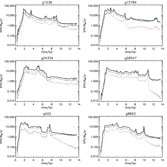
Figure 2: Star formation histories (SFHs) of the MUGS galaxies considered in this work. In each panel, the black solid lines are SFHs computed for all the stars inside $R_{vir}$. The blue dashed lines and the red dotted lines are the SFHs for stars belonging to the disc and the bulge, respectively, after performing a kinematic cut as described in Sect. 2.2.

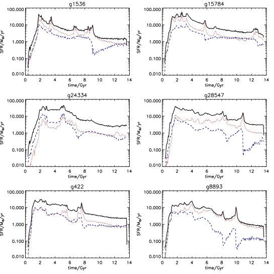
Figure 3: Star formation histories (SFHs) of the MUGS galaxies considered in this work. In each panel, the black solid lines are as in Fig.  2, whereas the blue dashed lines and the red dotted lines are the SFHs for stars belonging to the disc and the bulge, respectively, after performing a pure spatial cut as described in Sect. 2.3.

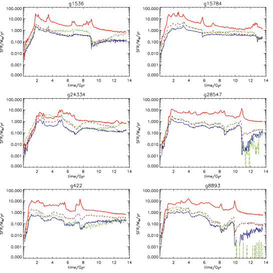
Figure 4: Star formation histories (SFHs) of the MUGS discs in different spatial regions. The red dashed lines, blue solid lines, and green dash-dotted lines represent the SFHs computed considering the star particles which at the present time are located at radii $r$$<$2 $R_{d}$, between 2 $R_{d}$ and 3 $R_{d}$, and radii $r$$>$3 $R_{d}$, respectively. To trace the SFH of the innermost disc regions, disc particles within typical bulge radii (i.e. at $r$$<$1-3 kpc) have been excluded. The thick solid red lines are pure spatially cut bulge SFHs, i.e. they represent SFHs calculated considering all the star particles in the innermost “bulge” regions, regardless of their kinematics.

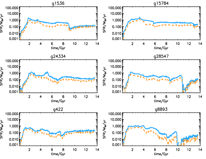
Figure 5: “Solar neighbourhood” star formation histories of the MUGS galaxies and effect of bulge stars with positive circularities. The solid lines are the SFHs calculated after a kinematic cut as described in Sect. 2.2 plus a spatial cut as in Sect. 2.3. The dashed lines are the result of a spatial cut and the exclusion of all the star particles with $J_{z}/J_{circ}(E)<0.8$.

3 Results

3.1 Star Formation Histories

In Fig. 2, the star formation histories (SFHs) of the six MUGS galaxies are shown. In each panel, we show the SFH computed considering all the star particles within the virial radius (solid lines), that of the disc (dashed lines), and the bulge (dotted lines). The disc and bulge SFHs reported in Fig. 2 have been derived after performing the kinematic decompostion described in Sect. 2.2.

All the SFHs show similar behaviour, i.e. an $\sim$20$-$30 M_⊙/yr peak during the first few Gyrs, followed by an exponential and fairly continuous decline at later times with a timescale ranging from $\sim$4$-$7 Gyr.

In two cases (g24334 and g422), the early evolutionary phases are dominated by more intense centrally-concentrated star formation. In the other systems, throughout their whole history (in general), the discs show SFRs higher than those of their associated bulges. Moreover, the disc SFHs show higher present-day SFRs than the bulges by factors of a few to ten. In a few cases, such as g1536, the bulge SFHs are somewhat higher than those encountered in nature, at least over the last $\sim$5 Gyrs of the simulation. In general, the present-day bulge SFRs are higher than those seen in the sample of Fisher et al (2009) by factors of a few, except for g28547, which sits at the median of the aforementioned sample. That said, it is important to remind the reader that in this suite of simulations, the only form for star formation ‘quenching’ present is that associated with feedback from SNe; in general, this is not sufficient for producing passive spheroids in cosmological simulations (e.g. Kawata & Gibson 2005) or semi-analytic models (e.g. Calura & Menci 2009).

In Fig. 3, we show the SFHs for discs and bulges obtained solely via the spatial cut criteria described in Sect.  2.3. All the MUGS galaxies suffer an excessive central concentration of mass and of star formation, as already reported by Stinson et al. (2010), who performed a careful analysis of the rotation curves of various systems, and of Pilkington et al. (2012a), who studied the radial metallicity gradients.

As Fig. 3 shows, if we assume that all the star particles included within the innermost 1-3 kpc belong to the bulges, we end up with unnaturally high present-day values for the bulge SFHs, which reflect this well-known issue of an excess of mass in the centre of the simulated galaxies. Several works have already shown that the problem regarding the central concentration of mass may be partially alleviated by increasing the simulation resolution (e.g. Pilkington et al. 2011; Brook et al. 2012). Further tests are needed to understand to what extent resolution may help in ameliorating this problem.

As reported by Stinson et al. (2010), in general MUGS bulges are bluer than real bulges, and that quenching star formation sooner would produce bulges that better match the red sequence. In fact, MUGS galaxies do not include AGN feedback, which might significantly help driving star-forming gas out of the central regions of galaxies and limiting the mass of bulges, as already shown in semi analytic models and even on mass scales comparable to the one of the MW bulge (e.g., Calura & Menci 2011).

In Fig. 4, we show the SFHs for different spatial regions within each of the galaxies in our sample. For each stellar particle, we have calculated its present-day distance from the centre of the disc and divided the disc into three different regions: (1) the innermost one, in which all the particles lie within the inner 2 $R_{d}$, excluding those in disc regions within radii typical of bulges (1-3 kpc); (2) an annulus encompassing the particles with distances 2 $R_{d}$$<$$r$$<$3 $R_{d}$, and (3) the disc outskirts, including all the particles with distances beyond 3 $R_{d}$.

In each panel of Fig. 4, the thick solid red lines represent pure spatially-cut bulge SFHs, i.e. SFHs calculated considering all the star particles in the innermost “bulge” regions, regardless of their kinematics. It is important to note that in Fig. 4 we are showing SFHs calculated in different spatial regions considering the present-day position of each stellar particle, and not the position where the stellar particles were formed. The bulge SFHs dominate the overall star formation budget througout most of the cosmic time.

After having excluded the star particles in the bulge regions, the SFHs of the innermost disc regions are in general comparable to those at larger distances. At late times, the outermost parts tend to show ‘oscillating’ SFHs at late times ($>$5 Gyrs). This effect is due to the adoption of a star formation density threshold ($>$1 cm^-3); the outermost regions of the discs are characterised by lower densities, hence more likely to present such a modulating star formation behaviour, once the gas density is comparable to that of the threshold value. This phenomenon can also be seen in non-cosmological chemical evolution models for disc galaxies (e.g. Chiappini et al. 2001; Cescutti et al. 2007) which adopt a density threshold for star formation. We refer the reader to a more targeted analysis of the temporal evolution of the radial star formation rate profiles within simulated cosmological discs by Pilkington et al. (2012a). It is also important to recall that radial migration is likely to occur within these simulations. Sanchez-Blazquez et al. (2009) presented the analysis of a cosmological disc simulation, comparable in mass and kinematic heating profile (e.g. House et al. 2011) to those analysed here, and found that the mean radial distance traversed by the disc star particles was $\sim$1.7 kpc. The effects of stellar migration are not taken into account in Fig. 4.

To assess the effect of bulge stars with positive circularities, in Fig.  5 we show the “solar neigbourhood” SFHs computed as in Fig. 4, compared to the SFHs computed considering the star particles with 2 $R_{d}$$<$$r$$<$3 $R_{d}$ and having excluded the ones with $J_{z}/J_{circ}(E)<0.8$. As visible in Fig. 1, at this $J_{z}/J_{circ}(E)$ value the bulge circularity distribution is very low, whereas the one for the disc is close to the peak value. This ensures the removal of a substantial fraction of particles with bulge kinematics, while at the same time, retaining the majority of disc particles.

The difference bewteen the two SFHs is in most of the cases more visible at early (i.e. $<$ 8 Gyr) times, when the bulge SFH was particularly intense, as seen in Fig.  4. Overall, the exclusion of star particles with $J_{z}/J_{circ}(E)<0.8$ does not seem to affect the global shape of the SFHs.

In the current analysis, the use of a spatial or kinematical definition of the solar neighbourhood region does not substantially affect our results on the metallicity distribution. There is a low contamination from low angular momentum, high metallicity bulge star particles at large distances from the centre. The effects of bulge stars with positive circularities on the solar neighbourhod MDF will be studied in detail later in Sect. 3.3.

3.2 Metallicity Distribution Functions in the Discs

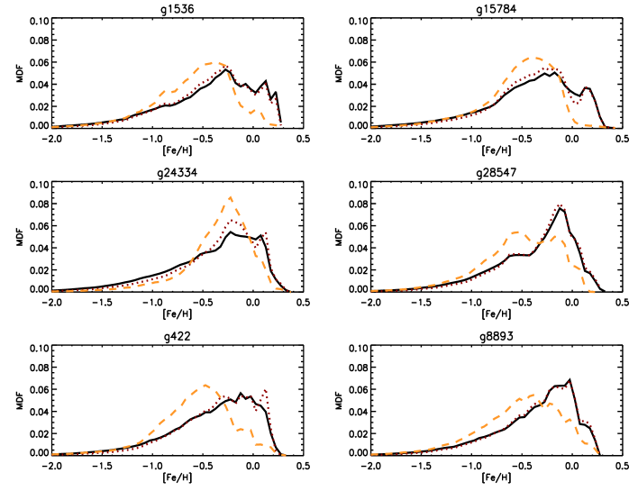
Figure 6: Metallicity distribution functions for the six MUGS discs. Thick solid lines: MDF calculated considering all the stellar particles within the virial radius. Thin dotted lines: MDFs for the particles belonging to the discs after the kinematic decomposition described in §2.2. Thin dashed lines: MDF calculated for particles in the disc and after the additional spatial cut described in §2.3, i.e. considering the star particles in the disc within 4 kpc of the mid-plane and at galactocentric radii R$\geq R_{b}$.

In Fig. 6, we show the MDFs of our six simulated galaxies. In each panel, we show the MDF calculated using all the stellar particles (i) located within the virial radius $R_{vir}$, (ii) in the disc after the kinematic decomposition described in Sect.  2.2 and (iii) after a kinematic descomposition plus a spatial cut as described in Sect.  2.3.

The MDFs for the particles included within $R_{vir}$ show several peaks, each corresponding to stellar populations associated with various kinematic components. A representative case is that of our fiducial simulation g15784, whose MDF shows a high-metallicity peak at [Fe/H]$\sim$0.2 and a broader, more significant, peak at lower metallicity (near [Fe/H]$\sim$$-$0.2). The disc MDFs are in most cases very similar to the ones calculated using all the star particles within $R_{vir}$.

Performing the spatial cut of §2.3, we can see that the high-metallicity peak of the MDF has been removed (g1536 and g15784) or substantially reduced (g28547). This is because in any galaxy, the highest metallicity stellar particles tend to reside near the centre, similar indeed to what is encountered in nature, including our own Milky Way, where the metal-rich stars are found preferentially in the bulge and inner disc.

In some cases (g28547 and g8893), the multi-peaked structure of the MDF is still present (or even exacerbated) after performing the spatial cut. This is due to their particular SFHs, which tend to show several late-time star formation episodes. A similar behaviour was found for dwarf galaxies within a semi-analytic galaxy formation model (Calura & Menci 2009), where multi-peak SFHs tend to be associated with complex multi-component stellar metallicity distributions.

Finally, we stress that a comprehensive analysis of the origin of the metallicity gradients in the MUGS discs, including a few cases described here, can be found in Pilkington et al. (2012a). In general, MUGS galaxies can account for the slope of the metallicity gradient observed today in young stars in the Milky Way and in HII regions in local discs. The analysis of Pilkington et al. (2012a) showed that the metallicity zero-point of the MUGS galaxies is offset by 0.2-0.3 dex from those in nature, but this does not impact on the determination of the gradients therein.

3.3 Metallicity Distribution Functions in the Solar Neighbourhood

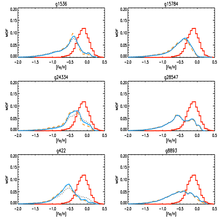
Figure 7: Metallicity distribution functions for the ’solar neighbourhood’ of each of the six MUGS discs, compared to the MDF observed in the solar neighbourhood as for the ’clean’ sub-sample drawn from the Geneva-Copenhagen Survey (Holmberg et al. 2009). The solid histrograms represent the observed MDF. The solid lines are MDFs calculated after a kinematic cut as described in Sect. 2.2 plus a spatial cut (i.e. considering an annulus encompassing all the particles with distances $r$ from the centre in the range 2 $R_{d}$$<$$r$$<$3 $R_{d}$) as in Sect. 2.3. The Dashed lines are MDFs after a spatial cut and the exclusion of all the star particles with $J_{z}/J_{circ}(E)<0.8$. Dotted lines: MDFs obtained with a solely spatial cut, i.e. considering the star particles in the annulus without any other kinematical selection.

In Fig. 7, we show the MDFs calculated for each simulation using star particles situated within a circular annulus of 2$R_{d}$$<$$r$$<$3$R_{d}$, compared with the observational MDF in the solar neighbouhood. The observational MDF adopted here is calculated from the Geneva Copenhagen survey (GCS) sample of solar-neighbourhood stars (Nordström et al. 2004; Holmberg, Nordström & Andersen 2007). Nordström et al. (2004) obtained Strömgren photometry and radial velocities for a magnitude-limited sample of $\sim$17000 F and G dwarfs. From the photometry, they estimated metallicities and ages. There has been some debate about the calibration of the metallicities and ages (Haywood 2006; Holmberg et al. 2007; Haywood 2008, Casagrande et al. 2011). Recently, the re-calibrated data from Holmberg et al. (2009) became available, and it is with the MDF drawn from these data that we compare our model predictions. Following Holmberg et al. (2009), we define a ’clean’ sub-sample by removing (i) binary stars, (ii) stars for which the uncertainty in age is $>$25%, (iii) stars for which the uncertainty in trigonometric parallax is $>13$%, and (iv) stars for which a ’null’ entry was provided for any of the parallax, age, metallicity, or their associated uncertainties. This ’clean’ sub-sample consists of $\sim 4000$ stars.

The region including the star particles with distances $r$ in the range 2$R_{d}$$<$$r$$<$3$R_{d}$ are analogous ‘solar neighbourhoods’ for the MUGS simulations; in the following, we will employ the MDF calculated for the star particles included in these region for our comparison with extant data of the Milky Way’s solar neighbourhood.

The solid lines in Fig.  7 are the MDFs calculated after a kinematic cut as described in Sect. 2.2 plus a spatial cut as explained in Sect. 2.3. The dashed lines are MDFs after applying a spatial cut and by excluding all the star particles with $J_{z}/J_{circ}(E)<0.8$. A comparison of the solid and dashed lines helps in understanding the role of bulge stars with positive circularities in the ’solar neighbourhood’ MDF: in all the panels, the MDFs computed in these two different ways are very similar, hence the contribution from bulge star particles at radial distances $>2R_{eff}$ is expected to be low. Also the MDFs computed by means of a solely spatial cut (dotted lines in Fig.  7) are very similar to the ones computed with a spatial plus kinematic cut. This shows that our results concerning the “solar neighbourhood” MDF are not overly sensitive to a kinematic selection of disc stars. This is an encouraging aspect, since for the observational sample we are comparing our results with, it is impossible to perform any such distinction between bulge and disc stars. The fact that the results are stable against the definition of “solar neighbrouhood” indicates that our results should be considered robust.

Concerning the comparison between model results and the observed MDF (solid histograms in Fig.  7), the first striking difference regards the position of the peak metallicities, with the model MDFs peaking at [Fe/H] values $\sim 0.2-0.3$ dex lower than the one of the GCS sample. This is an indication that the average stellar metallicity in the simulations is lower with respect to the one observed in the solar neighbourhood. Another important aspect emerging from this comparison regards the relative fraction of low metallicity stars, which in the simulated galaxies is substantially higher, and which will be quantified and discussed in more detail in Sect. 3.5.

3.3.1 Statistical analysis of the MDF in simulations and in the solar neighbourhood

A comparison of the main statistical features of the predicted MDFs and the empirical MDF of the Milky Way’s solar neighbourhood is provided in Tab. 2. The characteristics noted there are patterned closely upon those performed by Kirby et al. (2011) in their analysis of the MDFs of Local Group dwarf spheroidals and by Pilkington et al (2012b) in their analysis of the MDFs of simulated dwarf disc galaxies. In the second and third columns, we list the mean and the median of the MDF for a given simulation, whose name is reported in the first column. In this table, we use 5-$\sigma$ clipping of outliers from the distribution before deriving MDF shape characteristics. The dispersion $\sigma$ is reported in the fourth column, whereas the interquartile range (IQR), the interdecile (IDR), intercentile range (ICR), inter tenth percent (ITR), the skewness, and the kurtosis are reported in the fifth, sixth, seventh, eigth, ninth amd tenth columns, respectively. The dispersion $\sigma$, the IQR, IDR, ICR and ITR are different measures of the width of the distribution, while the skewness is a measure of the symmetry, with positive and negative values indicating an MDF skewed to the right (towards positive metallicities) and to the left (towards negative metallicities), respectively. The kurtosis (or peakedness) indicates the degree to which the MDF is peaked with respect to a normal distribution: high kurtosis values ($\gg 1$) signify a distribution with extended tails, while lower values signify light tails.

As already noted, the model MDFs show median metallicities that are systematically lower than the empirical MDF, with offsets ranging from $-$0.14 dex (considering the median as representative of the peak position) to $-$0.45 dex. In the fiducial simulation (g15784), the offset between the peaks is $-$0.32 dex.

The discrepancy is lower for g24334, for which we are only considering the innermost regions since its disk scalelength is only 1 kpc. It is therefore not surprising that the mean and median stellar metallicities for this system are larger with respect to the others, due to the presence of a significant metallicity gradient (Pilkington et al. 2012a), a point to which we return below.

3.3.2 Possible reasons for the discrepancies between simulations and observations

The apparent discrepancy between the MDF peaks of the simulated ’solar neighbourhood’ and that observed in the Milky Way can be ascribed to several reasons. First, the chemical evolution prescriptions incorporated within Gasoline (Raiteri et al. 1996) predict the cumulative Fe mass produced after 10 Gyr by a 1 $M_{\odot}$ simple stellar population, employing a Kroupa et al. (1993) IMF is 0.0007 M_⊙, a factor of two lower than that reported by Portinari et al. (2004), in their study of the impact of the IMF on various local chemical evolution observables. This discrepancy is due in part to a different SNeIa frequency (7% in the case of Portinari et al. 2004 versus 5% adopted within Gasoline), and to a lower Fe yield from SNeII (in Gasoline, SNeII form a $1M_{\odot}$ SSP produces 0.00022 M_⊙ of Fe, versus 0.00048 M_⊙ according to Portinari et al. 2004) and to a slightly lower mass of Fe produced by a single SNIa (0.63 M_⊙ versus 0.7 M_⊙ used by Portinari et al. 2004). Therefore, the nucleosynthesis prescriptions adopted within Gasoline tend to produce less Fe with respect to other chemical evolution models designed to reproduce local constraints, and this is certainly one of the reasons for the lower metallicity peaks of the simulated MDFs. Another reason is linked to the formalism used here to model SNeIa: here, the contribution of SNeIa progenitors with mass $m$$<$1.5 M_⊙ was neglected, and this leads to the underestimation of the Fe mass in stellar particles older than 5 Gyr. In fact, by integrating the type Ia SN rate of Greggio & Renzini (1983) from $T_{0}$=0 Gyr to $T_{1}$=5 Gyr, corresponding to the lifetime of a 1.5 M_⊙ star, and comparing this number to the integral of the rate over one Hubble time, one can show that the total Fe production from stars down to the present turnoff mass (0.8 M_⊙) is underestimated by $\sim$0.1 dex.

Other effects which could cause a loss of metals and a consequent low stellar metallicity in the disc would be metal ejection during mergers occurring at early times. In this case, we should be finding mean metallicities higher in the gas (including both cold and warm components) with respect to the stars. However, a preliminary estimate of gas and stellar metallicity gradients in the simulated discs do not seem to support this scenario: in the g15784 simulation, the mass-weighted average metallicity calculated for the gas particles belonging to the most massive galaxy (i.e. the g15784 disc) is $<Z>_{g}=0.0005$, whereas the analogous stellar mean metallicity is $<Z>_{*}=0.007$.

Finally, as indicated by a parallel study of the evolution of the metallicity gradients in the MUGS galaxies (Pilkington et al. 2012a), the star formation threshold may contribute to a more centrally concentrated star formation history, in particular during the early stages. If star formation in the disk is underestimated in the models at early times, this may lead to steep abundance gradients and low metallicity star formation in the early disc, resulting in a lower present-day metallicity in this region.

The model MDFs appear broader than the observed one, as indicated by the $\sigma$, IDR-ITR values. This could be related to radial migration of stellar particles, which can broaden the MDF (Schoenrich & Binney 2009) and whose effect could be enhanced by the fact that these simulations (like most cosmological disc simulations) are substantially hotter (kinematically speaking) relative to the Milky Way (e.g. House et al. 2011). Metal circulation in the disc and outwards could play some role as well in broadening the MDF.

The skewness values vary from disc to disc, however, in most cases, the simulated MDFs tend to show more negative skewness with respect to the observed MDF of the solar neighbourhood, which relates mostly to their over-populated low-metallicity tails.

Finally, the kurtosis values are higher than the one derived for the GCS sample, again due to heavy low metallicity tails. It is worth noting that the use of a 5-$\sigma$ clipping limits the effects of the presence of extreme low-metallicity tails which, without taking into account any clipping, would give rise to even higher kurtosis values.

Later in Section 3.6, we will see how the age-metallicity relation may be regarded as a useful diagnostic to understand in better detail the implications of our MDF study and the reasons for the discrepancies between the theoretical and obserevd MDFs.

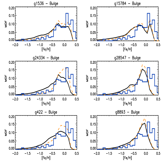
Figure 8: Metallicity distribution functions for the bulges of each of the six MUGS galaxies. Solid lines: MDFs calculated by using all the particles belonging to the spheroid, after application of the kinematic decomposition described in §2.2. Dashed lines: spheroid MDF restricted to the innermost regions of the bulge, i.e. computed by performing a spatial cut on the bulge component. In each panel, the solid histogram is the observational bulge MDF from Zoccali et al. (2008).

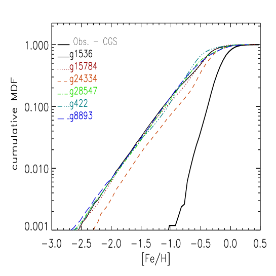
Figure 9: Cumulative metallicity distribution functions for the ’solar neighbourhood’ of each of the six MUGS galaxies and for the CGS ’clean’ sub-sample, each one normalized at the integral of the corresponding differential MDF.

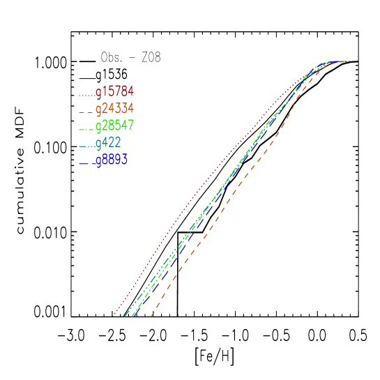
Figure 10: Cumulative metallicity distribution functions for the bulges of each of the six MUGS galaxies and for the Z08 sample. Each cumulative MDF is normalized to the integral of the corresponding differential MDF.

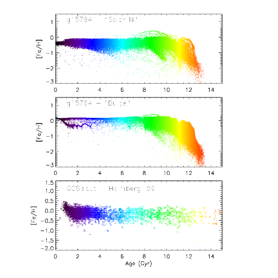
Figure 11: Age-metallicity relations for the “solar neighbourhood” (upper panel) and of the “bulge” (middle panel) of the simulated galaxy g15784, and of the sub-sample of Holmberg et al. (2009) of solar neighbourhood stars described in Sec. 3.3. The colours of each simulated or observed star scales with its age (colour bar on the right).

3.3.3 Possible selection effects in the observed sample

In principle, two possible kinds of bias may affect the comparison between data and simulations. One is connected with the observational uncertainties and the sample selection, the other involves the ”representativeness” of the local sample. Concerning the former, the ’clean’ sample of Holmberg et al. (2009) is complete down to $M_{V}\sim 4.5$ up to about 40-50 pc, thus no significant fraction of F-G stars is expected to be missed. In principle, the choice of using F-G stars (which are long-lived enough to trace the disk star formation over the entire Hubble time) may imply a slightly different range of masses for populations of different metallicities (a metal poor star is hotter than a metal rich star, so for a fixed spectral type it will be slightly less massive), but this effect is likely to be very small and it is unlikely to substantially affect our analysis.

The other potential issue stems from the definition of ”solar neighborhood” itself. Dynamical diffusion of orbits allows stars to drift from their birthplaces over time scales of several Gyr and, as a consequence, may deplete the local (i.e. regarding the volume within $\sim 100$ pc) star formation rate at early epochs (see e.g. Schröder & Pagel 2003). Indeed, different thin disk populations are known to have different scale heights, with their height increasing with age. Since oldest stars are likely the most metal poor, this could imply an observed local metallicity distribution biased against lowest metallicity stars.

It is not possible to assess quantitatively the role of each of the effects described in this section. Important constraints may come from the Gaia mission, which will soon take a complete census of stars down to ${M}_{V}=4.5$ with parallaxes measured with an accuracy better than 10% up to 2–3 kpc, thus extending the solar neighborhood sample to a realistic disk/thick disk sample.

3.4 Metallicity Distribution Functions in the Bulge

The bulge MDFs for the six MUGS galaxies are shown in Fig 8, together with observational data from Zoccali et al. (2008, Z08 hereinafter). The latter are derived from a survey of 800 K-giants in the Galactic bulge, observed at a resolution $R$$\sim$20000. In each panel, we show two MDFs derived from the simulations: one based upon the use of all star particles belonging to the bulge, after application of the kinematic decomposition described in §2.2 (solid lines), and a second restricted to the innermost regions of the bulge, i.e. computed by performing a spatial cut on the bulge component (dashed lines). As described in §2.3, the stellar particles belonging to the bulge region are those at a distance $r=\sqrt{X^{2}+Y^{2}+Z^{2}}$ $<$ $R_{b,cut}$ (where, 1$<$$R_{b,cut}$$<$3 kpc).

The main features of the observed MDF for the Galactic bulge and those derived from the simulations are summarised in Table 3. The entries reported in the columns of Table 3 are the same as those of Tab.  2, shown in the same order. Both the empirical and simulation-based MDFs show negative skewness, and are more asymmetric than the corresponding MDFs for the solar neighbourhood. The empirical MDF of Zoccali et al. (2008) shows a peak centered nearly at solar [Fe/H] and broader than the one of the solar neighbourhood. The bulge MDF also possesses a negative skewness as the solar neighbourhood. The higher kurtosis of the bulge MDF indicates a more peaked metallicity distribution with respect to that of the solar neighbourhood.

In most of the cases, the peak of the model MDF, represented by the mean and median values reported in Tab. 3, is offset with respect to the empirical one by $-$0.2 - $-$0.3 dex; such an offset is perhaps not surprising, considering the implementation of the stellar yields, as discussed in §3.3. The discrepancy is lower only for g24334, a simulation for which the stars accreted from disrupted satellites dominate over the ones formed in its main disc and one whose radial abundance gradient is both steep and shows little temporal evolution, while the others (e.g. g15784 and g422) show gradients which flatten with time (Pilkington et al. 2012a). Only  g24334 shows the same steep radial gradient today as it showed at redshift $z$$\sim$2.5, leading in part to higher overall metallicity in its innermost regions, which are the ones we are considering as “solar neighbourhood” owing to its small disc size. In all these senses, g24334 differs from the other five MUGS simulations, which each show similar mean and median [Fe/H] values. The dispersions of the simulated bulge MDFs are, in general, in better agreement with the observations than the case of the solar neighbourhood MDFs. A good agreement between model predictions and observations is visible also for the skewness values. The kurtosis values are still higher than the one of the observed bulge MDF, however the agreement is better than in the solar neighbourhood.

Two recent studies of red giants in Baade’s Window (Hill et al. 2011) and dwarf/subgiants in the Galactic bulge (Bensby et al. 2011) suggest that the MDF in the inner region has multiple peaks (or is at least double-peaked), with a low-metallicity peak occuring near [Fe/H]$\sim$$-$0.6 (Bensby et al.) or [Fe/H]$\sim$$-$0.3 (Hill et al.), and a higher-metallicity peak centered at [Fe/H]$\sim$$+$0.3. Hill et al. suggest that the low-metallicity stellar component shows a large dispersion, while the high-metallicity component appears narrow.

The above results are in qualitative agreement with those shown in Fig 8, in particular as far as the Milky-Way analogue g15784 is concerned. A low-metallicity component peaked at [Fe/H]$\sim$$-$0.3 showing significant dispersion is visible in the top-right panel of Fig 8, with a narrower component centered near [Fe/H]$\sim$$+$0.15. The relative amplitude of the two peaks in g15784 is close to unity, while the aforementioned studies of Hill et al. (2011) and Bensby et al. (2011) suggest that the lower-metallicity peak appears considerably weaker than the one at high-metallicity. Both studies converge to a picture of a longer formation time-scale for the metal-rich component. Such a picture is consistent with the age-metallicity relation predicted for the bulge of g15784, (see Sect. 3.6), and with the star formation histories shown in Fig 1.

From Fig 1, it is clear that the peak of the star formation occurs at early times. Additionally, while residual star formation is present at relatively recent times, this does not contribute to the bulk of the stellar mass, i.e. most of the stars in the simulated bulges are old and have low metallicity.

Another aspect emerging from the studies of Hill et al. (2011) and Bensby et al. (2011) is the uncertainty in the position/metallicity of the metal-poor stellar component, likely due to the very different sample selection criteria between the two studies. For the moment, we do not attempt to perform any more detailed comparison with these results since they are very recent and awaiting further confirmation.

3.5 The Cumulative Metallicity Distribution

A diagnostic often used to investigate in better detail the low metallicity tail of the MDF in chemical evolution models is the cumulative metallicity distribution function. The cumulative MDF, calculated at a given metallicity [Fe/H], represents the number of stars with metallicity lower than [Fe/H].

The cumulative MDF reflects essentially the same information as the differential MDF (Caimmi 1997), but it is less sensitive to small number statistics and better tracks the behaviour at low metallicties for both low-metallicity local galaxies (Helmi et al. 2006) and the solar neighbourhood. In Fig. 9, we show the cumulative MDF as observed in the solar neighbourhood and as predicted for the six MUGS galaxies. In Fig.  9, each curve is normalized to the integral of the corresponding MDF.

From the upper of Fig 9, one can see that in the Milky Way’s solar neighbourhood, from the sample of Holmberg et al. (2009) and with the cuts performed in Sect. 3.3, $\sim$10% of the stars have a metallicity [Fe/H]$<$$-$0.5. This is in stark contrast with the simulation results which, without taking into account colour and magnitude selection effects, below [Fe/H]=-0.5 show fractions greater than $\sim$30%.

Mass fractions relative to the total MDF for the stars associated with the four metallicity values are tabulated in Tab.  4, where the excess of low metallicity stars is emphasised: at any metallicity value from [Fe/H]=-2 to [Fe/H]=$-0.13$, the predicted mass fraction is considerably higher than the values obtained by integrating the observational MDF. This discrepancy is certainly related to the metallicity offset visible in the peaks of differential MDF discussed in Sect. 3.3. However, the excess of very low metallicity stars is to be ascribed to other reasons. Several solutions to this problem could be plausible: one of them is the adoption of a modified IMF, known to alleviate the excess of metal-poor stars in local dwarf galaxies - (see e.g., Calura & Menci 2009). However, since this would cause a larger relative number of high mass stars in a stellar population, this modified IMF would have a strong impact on the abundance ratios, such as the [O/Fe] ratio, and even on the SN feedback. In the solar neighbourhood, an IMF similar to that of Kroupa et al. (1993), as adopted here, reproduces a large set of observational constraints, including the abundance ratios (Calura et al. 2010). Further, since a truncated or even slightly top-heavy IMF is known to produce a strong $\alpha$ enhancement in the abundance ratios (Calura & Menci 2009), this does not seem to represent a proper solution to our problem. Investigations of the abundance ratios in the solar neighbourhood of the MUGS discs will be a useful to test this hypothesis as a solution to the problem related to the excess of metal-poor stars. Such an analysis is currently underway, but deferred to a forthcoming paper.

An alternate explanation to the dearth of low metallicity stars in the solar neighbourhood is to invoke a prompt initial enrichment scenario, with a population of objects such as zero metallicity (Pop III) stars (Matteucci & Calura 2005; Ohkubo et al. 2006; Greif et al. 2007), releasing a sufficient amount of heavy elements to prevent the formation of very low-metallicity stars in galactic discs. Testing the impact of such objects in the chemical enrichment of discs in simulations would be possible by including the yields of very massive stars as provided by, e.g. Ohkubo et al. (2006). This is beyond the scope of the present paper, but under consideration for a future generation of chemo-dynamical simulations.

In Fig. 10, we show the cumulative predicted bulge MDF for our MUGS galaxies and that observed in the Galactic bulge by Zoccali et al. (2008), with each cumulative MDF normalized to the integral of the corresponding differential MDF. The mass fractions relative to the total MDF for the stars associated with the various metallicity values are tabulated in Tab.  5. Also in the bulges the simulated galaxies overestimate the number of low metallicity stars at most metallicities. However, aside from the overabundance of low-metallicity stars, the rest of the form of the model MDF is quite consistent with the observational MDF of Z08. Again, it will be interesting to see in the future if the predicted overabundance of low metallicity stars is due to sampling effects in the observational MDF and if this could be alleviated with different nucleosynthesis prescriptions for zero metallicity stars.

3.6 The Age-Metallicity Relation

In Fig. 11, we are showing the age-metallicity relation (AMR) in the “solar neighbourhood” of our fiducial Milky Way analogue g15784 (upper panel), of its bulge (middle panel) and of our GCS ’clean’ sub-sample (lower panel). From this figure, it is possible to appreciate how the slope of the AMR is reflecting the MDF problems described in the previous sections, in particular the over-populated low metallicity tails visible in the theoretical MDFs and their negative skewness (see also the parallel study of the MDF in dwarf spiral galaxies of Pilkington et al. 2012b).

In Fig. 11, the metallicities of the stars in the Milky Way’s solar neighbourhood (GCS) are higher than those of the g15784 “solar neigbourhood”. This should not be surprising, in the light of the discussion in Sect. 3.3, in particular regarding the MDF peak metallicity of our simulations, lower than the one of the GCS.

A striking feature of Fig. 11 is that the AMR of the GCS solar neighbourhood sub-sample is essentially flat. The AMR predicted for the g15784 solar neighbouhood is predominantly flat, but significant deviations are clearly visible at ages $>10$ Gyr, where the g15784 simulation shows essentially a correlated AMR. In shape, this relation is similar to those predicted by classical galactic chemical evolution models (e.g. Fenner & Gibson 2003, Haywood 2006; Spitoni et al. 2009).

These hints for a correlated AMR are to be associated to the excessive negative skewed MDFs of the simulations: the excessively negative skewness is mostly due to low metallicity star particles with ages $>10$ Gyr, older than the stars which settle on the plateau of AMR relation.

Furthermore, the dearth of stars older than 13 Gyr is striking as well, and is at variance with the results of non-cosmological homogeneous galactic chemical evolution models (Matteucci et al. 2009), which in general are successful in reproducing the local MDF. Perhaps more hints on this aspect could come from studies with inhomogenous chemical evolution models (Oey 2000; Cescutti 2008) , which allow to explore the parameter space nearly as fast as homogeneous models, but more suited to explore the causes of asymmetric or multi-peaked MDFs or the dispersion and slope of the AMR.

Also the bulge of g15784 sees a flat age-metallicity relation for stars born with [Fe/H]$\sim$$+$0.15. The formation of these stars, which would populate the high-metallicity peak in the bulge MDF, extends over a period of $\sim$10 Gyrs or more. Most of the stars older than $\sim$10 Gyrs have clearly formed with a lower metallicity and present a correlated AMR similar to the solar neighbourhood of g15784 . A more-thorough study of the AMR of MUGS simulations in both bulges and discs will be presented in Bailin et al., in prep.

3.7 MDFs of In-situ Stars vs Accreted Stars

Important clues as to the origin of various stellar populations formed at different metallicities may come from the study of the separate MDFs of the stars born in situ as opposed to those accreted (Sales et al. 2009; Roskar et al. 2008; Sanchez-Blazquez et al. 2009; Rahimi et al. 2010). We define in situ stars as being those born within a cylinder with a radius linearly increasing with cosmic time, constrained to a present-day current value of $\sim$30 kpc, with a time-independent height of $\pm$2 kpc (House et al. 2011). The choice of these values for radius and height were suggested after visual inspection of the appearence of the galactic disc at various cosmic times and redshifts. The choice for the height does not have any impact on our results (for values on the order of a few kpc); the value chosen is conservative and satisfies our desire to exclude the effects of satellites. In other words, in situ stars are born ‘locally’, at small distances from the main progenitor, while accreted stars form within satellites and are accreted later. Such a cylindrical volume encompasses both bulge and disc stars; no kinematical distinction is performed in this case, hence our results are valid for the whole galaxy including all its kinematical components.

In this section, we will only show the results regarding our Milky Way fiducial (g15784) - partly because it does represent the best analogue to our own Galaxy (see also Brook et al. 2011; 2012), and partly because its output temporal cadence was the highest, ensuring the greatest wealth of data with which to work. We did examine all relevant metrics which could be derived with the more limited information available to us at the time of analysis and find that none of our results are tied to this one system. This is consistent with the results of Pilkington et al. (2012a), regarding the similarity of the metallicity gradients within the MUGS galaxies.

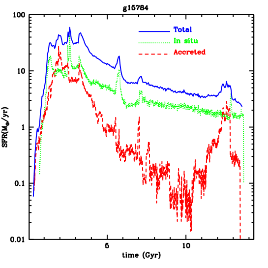
Figure 12: In situ (dotted line) vs accreted (dashed line) star formation history as a function of cosmic time for the MUGS galaxy g15784. The solid line corresponds to the the total (in situ + accreted) star formation history.

The SFHs of the stellar particles classified as in situ and accreted are shown for the MUGS galaxy g15784 in Fig. 12. The accreted stars form mostly at early times ($t_{\rm form}$$<$2 Gyrs, where the maximum of the ‘accreted’ SFH lies). Another peak within the ‘accreted’ SFH occurs more recently (12$\leq t_{\rm form}\leq$13 Gyr). The accreted stars contribute roughly 1/3 of the present-day stellar mass of the system; the majority of the stars are born in situ via a merger event and/or local star formation episode.

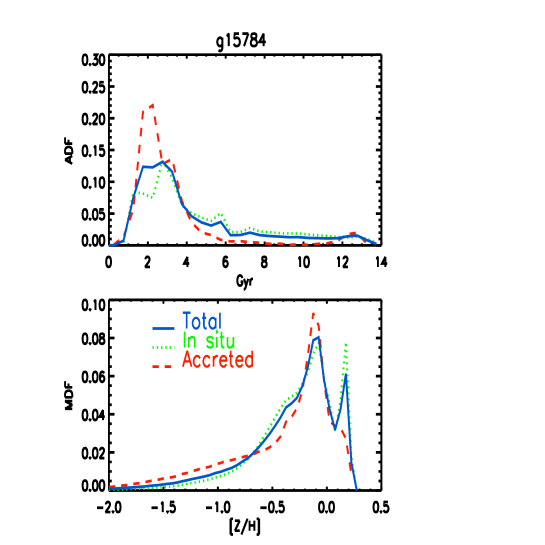
Figure 13: In situ (dotted line) vs accreted (dashed line) metallicity distribution functions (lower panel) and age distribution functions (upper panel) for the MUGS galaxy g15784. The solid lines correspond to the total (in situ + accreted) distribution functions.

In Fig. 13, we show the total MDF (solid lines in both panels, normalised to unity in all cases) for g15784, alongside the MDFs computed considering only the stars born in situ (dotted lines) and those accreted (dashed lines). We show here the MDFs based upon the total global metallicity Z, rather than just Fe, as the primary MDF metrics in which we are interested are insensitive to this choice.

The in situ MDF does not differ significantly from that of the total : both functions show two peaks (at [Z/H]=$-$0.2 and [Z/H]=$+$0.1). While we have not performed any kinematic decomposition here, it is quite obvious from the results discussed previously that the high metallicity peak is populated by the stars of the central region (i.e. bulge), whereas the lower-metallicity peak is generated by disc stars. The accreted stellar populations result in an MDF centered at [Z/H]$\sim$$-$0.1; furthermore, the MDF for accreted stars does not show any peak at higher metallicities present in the in situ MDF, and the low metallicity tail is more pronounced than that seen within the in situ population, indicating a larger relative fraction of low metallicity stars. It is not surprising that the accreted stars have lower metallicity, as they come from disrupted satellites which have lower mass than the central galaxy g15784, hence they should have lower metallicity stars, consistent with what the well-known mass-metallicity relation suggests in local and high-redshift galaxies (Maiolino et al. 2008; Calura et al. 2009).

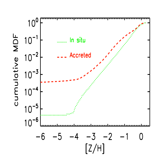
Figure 14: In situ (dotted line) vs accreted (dashed line) cumulative metallicity distribution functions for the MUGS galaxy g15784. The two curves are normalised to unity at [Z/H]=$+$0.5.

In the upper panel of Fig. 13, we show the age distribution function (ADF) of the stars born in situ and those accreted. The ADF shows that the accreted stars are mainly older than 10 Gyrs, whereas the stars formed in situ show a broad range of ages.
It is interesting to examine the cumulative MDF calculated for the stars born in situ and for those accreted (Fig. 14). The low metallicity tail (i.e. stars with [Z/H]$<$$-$4) is populated almost exclusively by accreted stars: this means that for g15784, the lowest metallicity stars are of extragalactic origin. We have investigated the kinetic energy of the stellar particles belonging to the two populations, but no clear distinction was found. This is consistent with that found by Rahimi et al. (2010), i.e. that an early accretion event is unlikely to leave any strong signature in any obvious physical property of the present-time stellar populations.

Table 2: Main features of the MDF observed in the Milky Way’s solar neighbourhood based upon the Holmberg et al. (2009) GCS empirical dataset and those of the simulated “solar neighbourhood” MDFs for the six MUGS galaxies.

	Mean	Median	$\sigma$	IQR	IDR	ICR	ITR	Skewness	Kurtosis
	[Fe/H]	[Fe/H]
Obs. MDF	-0.14	-0.12	0.18	0.23	0.44	0.92	1.42	-0.37	0.77
(GCS)
g1536	-0.56	-0.47	0.40	0.44	0.96	1.97	2.76	-1.12	1.82
g15784	-0.54	-0.46	0.37	0.40	0.88	1.89	2.90	-1.31	2.37
g24334	-0.43	-0.38	0.34	0.33	0.80	1.78	2.56	-1.29	2.74
g28547	-0.56	-0.53	0.40	0.51	0.99	1.91	2.71	-0.93	1.40
g422	-0.62	-0.58	0.36	0.37	0.82	1.97	2.84	-0.91	2.35
g8893	-0.55	-0.50	0.42	0.55	1.05	2.03	2.88	-0.85	1.19

Table 3: Main features of the MDF observed in the Milky Way’s bulge and those of the simlated “bulge” MDFs for the six MUGS galaxies.

	Mean	Median	$\sigma$	IQR	IDR	ICR	ITR	Skewness	Kurtosis
	[Fe/H]	[Fe/H]
Obs. MDF	-0.05	0.05	0.40	0.51	0.95	1.74	2.24	-1.23	1.89
(Z08,Baade’s window)
g1536	-0.29	-0.22	0.42	0.51	1.06	1.92	2.58	-1.23	1.75
g15784	-0.35	-0.28	0.45	0.58	1.11	2.02	2.72	-1.05	1.36
g24334	-0.16	-0.10	0.30	0.35	0.68	1.57	2.30	-1.42	2.80
g28547	-0.29	-0.19	0.34	0.39	0.81	1.70	2.48	-1.40	2.33
g422	-0.26	-0.17	0.36	0.43	0.86	1.74	2.55	-1.37	2.30
g8893	-0.27	-0.18	0.33	0.38	0.78	1.66	2.41	-1.40	2.45

Table 4: Cumulative MDF calculated at various metallicity values for the observed solar neighbourhood and for the solar neighbourhood analog sample of our six MUGS galaxies.

[Fe/H]	Obs.	g1536	g15784	g24334	g28547	g422	g8893
-2.000	0.000	0.006	0.006	0.003	0.006	0.006	0.006
-0.660	0.010	0.314	0.287	0.177	0.349	0.396	0.357
-0.450	0.048	0.524	0.513	0.395	0.587	0.701	0.547
-0.315	0.164	0.766	0.742	0.629	0.712	0.843	0.698
-0.130	0.446	0.898	0.915	0.831	0.843	0.920	0.830

Table 5: Cumulative MDF calculated at various metallicity values for the observed Bulge and for the “bulge” of our six MUGS galaxies.

[Fe/H]	Obs.	g1536	g15784	g24334	g28547	g422	g8893
-2.000	0.000	0.003	0.004	0.001	0.002	0.002	0.002
-1.230	0.015	0.041	0.052	0.013	0.025	0.025	0.022
-0.820	0.064	0.123	0.140	0.048	0.088	0.083	0.078
-0.351	0.211	0.304	0.388	0.159	0.271	0.263	0.255
0.050	0.549	0.817	0.807	0.813	0.947	0.873	0.923

4 Conclusions

We have analysed the MDFs constructed from a suite of six high-resolution hydrodynamical disc galaxy simulations. Both kinematic decompositions and spatial cuts were performed on each, in order to isolate samples of analogous ‘solar neighbourhood’ and ‘bulge’ samples, for comparison with corresponding datasets from the Milky Way. Our main conclusions can be summarised as follows.

• In general, after having performed a kinematical decomposition of discs and bulges, in most of the cases the star formation histories of the discs dominate over those of the bulges. On the other hand, if we define discs and bulges on a solely spatial basis, bulges have unnaturally high present-day SFR values , which reflect the well-known issue of an excessive central concentration of mass in the simulated galaxies. Increasing resolution may help alleviate this problem, however it is not yet clear to what extent.

• At the present time, an excess of star formation is visible in the simulated bulges. To limit this phenomenon, the next generation of simulations will have to include mechanisms of star formation quenching such as AGN feedback, which, in semi-analytic models of galaxy formation, have turned out to be efficient in decreasing star formation timescales in spheroids.

• The ‘oscillating’ behaviour of star formation in the outermost parts is due to the adopted star formation density threshold which acts to control the ability of the low-density regions in the outskirts to undergo substantial and sustained star formation.

• The MDFs derived using all the stellar particles situated within the virial radius possess a number of ‘peaks’, each associated with stellar populations belonging to various kinematic components. Applying a spatial cut, in particular removing central stars within $R_{b,cut}$=1$-$3 kpc from the centre, has a significant effect on the MDF in that the highest metallicity peak is generally removed. As in nature, these highest metallicity stellar particles tend to reside in the central region, on average.

• A region analogous to the solar neighbourhood was defined in each system, by considering all the star particles contained within an annulus 2$R_{d}$$<$$r$$<$3$R_{d}$. The MDF of these stars show median metallicities lower by 0.2$-$0.3 dex than that of the Milky Way’s solar neighbourhood. This can be traced to several reasons, including the lower stellar yields implemented within Gasoline. The predicted distributions are broader than the one observed in the solar neighbourhood, consistent with other studies of the MDF with cosmological simulations (Tissera et al. 2012). In our simulations, the overly broad MDFs are related to discs kinematically hotter relative to the Milky Way (House et al. 2011). The derived MDFs possess, on average, more negative skewness and higher kurtosis than those encountered in nature; such a result is traced to the more highly populated low-metallicity ‘tails’ in the simulations’ MDFs.

• The MDFs derived for stars in the bulges are in reasonable agreement with that observed in the Milky Way. While the median metallicities are somewhat lower, the inferred MDFs’ dispersions and skewness are consistent with the Milky Way. The kurtosis values are higher than the one of the observed bulge MDF, however the agreement is better than in the solar neighbourhood.

• The prevalence of the low-metallicity tails are emphasised by examining the cumulative MDFs. In the solar neighbourhood, the predicted relative number of stars with [Fe/H]$<$$-$3 with respect to the number of stars with [Fe/H]$<$$-$2 is of the order 10%, whereas in the Milky Way this ratio is effectively zero. Solutions to this problem include prompt initial enrichment by a population of short-lived zero metallicity stars or perhaps an alternate treatment of metal diffusion (Pilkington et al. 2012b).

• For the fiducial simulation (g15784), we studied the star formation history and the MDF of the stellar populations born in situ and of the those accreted subsequent to satellite disruption. An early accretion episode generated a population of stars older than $\sim$10 Gyrs, whereas the stars formed in situ show a broad range of ages. The low-metallicity tail of the MDF is populated mostly by accreted stars; this means that for g15784, the majority of the lowest metallicity stars are of extragalactic origin.

In the future, we plan to extend our study on the metallicity distribution function in MUGS galaxies to various kinematical components, including the halos, and to examine its variation with respect to position in the galaxy. A recent extensive work which will be useful to test our simulations is the one of Schlesinger et al. (2012), where by means of the SEGUE sample of G and K dwarf stars, the variations of the MDF in the Galaxy with radius and height has been investigated. A comparison of the results from various suites of disc galaxy simulations, such as Pilkington et al. (2012a), will be also useful to better understand the effects of the sub-grid physics on the MDFs.

References

- [] Abadi M. G., Navarro J. F., Steinmetz M., Eke V. R. 2003, ApJ, 591, 499
- [] Bensby T., et al., 2011, A&A, 533, 134
- [] Brook C. B., et al., 2011, MNRAS, 415, 1051
- [] Brook C. B., Stinson G., Gibson B. K., Roskar R., Wadsley J., Quinn T., 2012, MNRAS, 419, 771
- [] Caimmi R., 1997, AN, 318, 339
- [] Calura F., Menci N., 2009, MNRAS, 400, 1347
- [] Calura F., Menci N., 2011, MNRAS, 413, L1
- [] Calura F., Pipino A., Chiappini C., Matteucci F., Maiolino R., 2009, A&A, 504, 373
- [] Calura F., Recchi S., Matteucci F., Kroupa P., 2010, MNRAS, 406, 1985
- [] Casagrande L., Schönrich R., Asplund M., Cassisi S., Ramírez I., Melendez J., Bensby T., Feltzing S., 2011, A&A, 530, 138
- [] Cescutti G., Matteucci F., François P., Chiappini C., 2007, A&A, 462, 943
- [] Cescutti G., 2008, A&A, 481, 691
- [] Chiappini C., Matteucci F., Romano D. 2001, ApJ, 554, 1044
- [] Dotter A.; Chaboyer B.; Jevremovic D.; Kostov V.; Baron E.; Ferguson J. W., 2008, ApJS, 178, 89
- [] Fenner Y., Gibson B., 2003, PASA, 20, 189
- [] Few C. G.; Courty S.; Gibson B. K.;Kawata D.; Calura F.; Teyssier R., 2012, MNRAS, 424, L11
- [] Fisher, D. B.; Drory, N., Fabricius, M. H., 2009, ApJ, 697, 630
- [] Font A. S.; Johnston K. V.; Bullock J. S.; Robertson B. E., 2006, ApJ, 638, 585
- [] Freeman K., Bland-Hawthorn J., 2002, ARA&A, 40, 487
- [] Greggio L., Renzini A. 1983, A&A, 118, 217
- [] Greif T. H., Johnson, J. L., Bromm, V., Klessen, R. S., 2007, ApJ, 670, 1
- [] Haywood M., 2006, MNRAS, 371, 1760
- [] Haywood M., 2008, MNRAS, 388, 1175
- [] Helmi A., et al., 2006, ApJ, 651, L121
- [] Hill V., et al., 2011, A&A, 534, 80
- [] Holmberg J., Nordström B., Andersen J., 2007, A&A, 475, 519
- [] Holmberg J., Nordström B., Andersen J., 2009, A&A, 501, 941
- [] House E. L., et al., 2011, MNRAS, 415 2652
- [] Kawata D., Gibson B. K., 2005, MNRAS, 358, L16
- [] Kennicutt R. C., 1998, ApJ, 498, 541
- [] Kirby E. N., Lanfranchi G. A., Simon J. D., Cohen J. G., Guhathakurta P., 2011, ApJ, 727, 78
- [] Klypin A., Kravtsov A. V., Bullock J. S., Primack J. R., 2001, ApJ, 554, 903
- [] Kroupa P., Tout C. A., Gilmore G., 1993, MNRAS, 262, 545
- [] McMillan P. J., 2011, MNRAS, 414, 2446
- [] Maiolino R., et al., 2008, A&A, 488, 463
- [] Matteucci F., Brocato E., 1990, ApJ, 365, 539
- [] Matteucci F., Calura F., 2005, MNRAS, 360, 447
- [] Nordstöm B., et al., 2004, A&A, 418, 989
- [] Oey M. S., 2000, ApJ, 542, L25
- [] Ohkubo T., Umeda H., Maeda K., Nomoto K., Suzuki T., Tsuruta S., Rees M. J., 2006, ApJ, 645, 1352
- [] Pagel B. E. J., Tautvaisiene G., 1995, MNRAS, 276, 505
- [] Pilkington K., et al., 2011, MNRAS, 417, 2891
- [] Pilkington K., Few, C. G., Gibson B. K., et al. 2012a, A&A, 540, A56
- [] Pilkington K., Gibson B. K., et al., 2012b, MNRAS, accepted for publication (arXiv:1205.4796)
- [] Portinari L., Moretti A., Chiosi C., Sommer-Larsen J., 2004, ApJ, 604, 579
- [] Rahimi A., Kawata D., Brook C. B., Gibson B. K., 2010, MNRAS, 401, 1826
- [] Raiteri C. M., Villata M., Navarro J. F., 1996, A&A, 315, 105
- [] Roskar R., Debattista V. P., Quinn T. R., Stinson G. S., Wadsley J., 2008, ApJ, 684, L79
- [] Sales L. V. et al., 2009, MNRAS, 400, L61
- [] Sánchez-Blázquez P., Courty S., Gibson B. K., Brook C. B., 2009, MNRAS, 398, 591
- [] Schoenrich R., Binney J., 2009, MNRAS, 396, 203
- [] Schlesinger K. J., et al. 2012, ApJ, submitted, arXiv:1112.2214
- [] Schröder K. P., Pagel B. E. J., 2003, 343, 1231
- [] Spitoni E.; Matteucci F.; Recchi S.; Cescutti G.; Pipino A., 2009, A&A, 504, 87
- [] Stinson G., Seth A., Katz N., Wadsley J., Governato F., Quinn T., 2006, MNRAS, 373, 1074
- [] Stinson G. S., Bailin J., Couchman H., Wadsley J., Shen S., Nickerson S., Brook C., Quinn T., 2010, MNRAS, 408, 812
- [] Tinsley B. M., 1980, Fund. Cosmic Phys., 5, 287
- [] Tissera P., White S. D. M., Scannapieco C., 2012, MNRAS, 420, 255
- [] Wadsley J. W., Stadel J., Quinn T., 2004, New Astronomy, 9, 137
- [] Wielen R., 1977, A&A, 60, 263
- [] Woosley S. E., Weaver T. A. 1995, ApJ, 101, 181
- [] Zoccali M., Hill V., Lecureur A., Barbuy B., Renzini A., Minniti D., Gómez, A., Ortolani S., 2008, A&A, 486, 177 (Z08)