A study of Wigner functions for discrete-time quantum walks

Abstract

We perform a systematic study of the discrete time Quantum Walk on one dimension using Wigner functions, which are generalized to include the chirality (or coin) degree of freedom. In particular, we analyze the evolution of the negative volume in phase space, as a function of time, for different initial states. This negativity can be used to quantify the degree of departure of the system from a classical state. We also relate this quantity to the entanglement between the coin and walker subspaces.

I introduction

Quantum Walks (QW) are considered a as a piece of potential importance in the design of quantum algorithms Shenvi et al. (2003); Ambainis (2007); Childs et al. (2003); Childs and Goldstone (2004); Tulsi (2008), as it is the case of classical random walks in traditional computer science. As in the case of random walks, QW’s can appear both under its discrete-time Aharonov et al. (1993) or continuous-time Farhi and Gutmann (1998) form. Moreover, it has been shown that any quantum algorithm can be recast under the form of a QW on a certain graph: QWs can be used for universal quantum computation, this being provable for both the continuous Childs (2009) and the discrete version Lovett et al. (2010). Experiments have been designed or already performed to implement the QW Knight et al. (2003); Travaglione and Milburn (2002); Dür et al. (2002); Du et al. (2003); Ryan et al. (2005); Xue et al. (2008); Witthaut (2010); Schreiber et al. (2010); Xue et al. (2009); Zhao et al. (2007).

In this paper, we concentrate on the discrete-time QW on a line. We perform a systematic study making use of Wigner functions, which are defined for this problem. Wigner functions Wigner (1932); Hillery et al. (1984) were introduced as an alternative description of quantum states. They play an important role in quantum mechanics, having been widely used in quantum optics to visualize light states. From the experimental point of view, they provide a way for quantum state reconstruction via tomography and inverse Radon transformation Schleich (2001).

Wigner functions are quasi-probability distributions in phase space, meaning that they cannot be interpreted as a probability measure in momentum and space configurations. This is an obvious fact for any quantum description, and only marginal distributions can be associated to probabilities in position or momentum (or any linear combination, i.e. any quadrature). In fact, Wigner functions can take negative values, thus invalidating a direct link to a probability distribution. This caveat, however, turns out to be a potential advantage, for it can be used to identify “true” quantum states. More precisely, the volume of the negative part of the Wigner function, its negativity, has been suggested as a figure of merit to quantify the degree of non-classicality Kenfack and Zyczkowski (2004). This idea has been recently exploited Mari et al. (2011) to directly estimating nonclassicality of a state by measuring its distance from the closest one with a positive Wigner function.

When dealing with the discrete QW, one has to account for the extra degree of freedom (in addition to the spatial motion): the coin. We consider the simplest case of a two level coin. Therefore, the Wigner function has to incorporate this extra index and, with the prescription we use, it turns into a matrix. We will propose a rather straightforward extended definition of negativity for this Wigner “function”. Then the question arises, what kind of states of the QW are nonclassical? Does this quantumness increase in time, as the QW evolves through its unitary evolution? We want to explore these questions using the Wigner function. A different topic, although it is closely related to the previous one, is whether this nonclassicality can be related to the entanglement between the walker and the coin, since this quantity is also evolving during the QW evolution.

This paper is organized as follows. In Sect. II we review the main definitions pertinent to the QW on a line. Sect. III introduces the Wigner function for our problem and the main associated properties. We present some examples showing our numerical results for the Wigner function evolution in Sect. IV. In Sect. V we define an extension of the negativity to the QW, based on the proposal made in Kenfack and Zyczkowski (2004) for a scalar function. We end in Sect. VI by summarizing our main results and conclusions.

II Discrete-time QW walk on a lattice

The discrete-time QW on a line is defined as the evolution of a one-dimensional quantum system following a direction which depends on an additional degree of freedom, the coin (or chirality), with two possible states: “left” $|L\rangle$ or “right” $|R\rangle$. The total Hilbert space of the system is the tensor product $H_{s}\otimes H_{c}$, where $H_{s}$ is the Hilbert space associated to the lattice, and $H_{c}$ is the coin Hilbert space. Let us call $T_{-}$ ($T_{+}$) the operators in $H_{s}$ that move the walker one site to the left (right), and $|L\rangle\langle L|$ , $|R\rangle\langle R|$ the chirality projector operators in $H_{c}$. The QW is defined by

$$U(\theta)=T_{-}\otimes|L\rangle\langle L|\text{ }C(\theta)+T_{+}\otimes|R\rangle\langle R|\text{ }C(\theta),$$ (1)

where $C(\theta)=\sigma_{z}\cos\theta+\sigma_{x}\sin\theta$, and $\sigma_{z}$, $\sigma_{x}$ are Pauli matrices acting on $H_{c}$. For $\theta=\pi/4$ the operator $C(\theta)$ becomes the Hadamard transformation. The unitary operator $U(\theta)$ transforms the state in one time step as

$$|\psi(t+1)\rangle=U(\theta)|\psi(t)\rangle.$$ (2)

The state at time $t$ can be expressed as the spinor

$$|\psi(t)\rangle=\sum\limits_{n=-\infty}^{\infty}\left[\begin{array}[]{c}a_{n}(t)\\ b_{n}(t)\end{array}\right]|n\rangle,$$ (3)

where the upper (lower) component is associated to the right (left) chirality, and $\left\{\mid n\rangle/n\in\mathbb{Z}\right\}$ is a basis of position states on the lattice. A basis in the whole Hilbert space can be constructed as the set of states $\left\{\mid n,\alpha\rangle=\mid n\rangle\otimes\mid\alpha\rangle/n\in\mathbb{Z};\alpha=L,R\right\}$.

III Wigner functions for the quantum walk

An important tool in some fields related to quantum physics is the use of quasi-probability distributions. Wigner functions constitute the major example, although other functions as the Glauber-Sudarshan $P$ function Glauber (1963); Sudarshan (1963) or the Husimi $Q$ function Husimi (1940) are commonly used in quantum optics. For the case of a one-dimensional system with continuous position $x$ and conjugate momentum $p$, the Wigner function is defined as Wigner (1932):

$$W(x,p)=\frac{1}{\pi}\intop_{-\infty}^{\infty}\psi^{*}(x-y)\psi(x+y)e^{-2ipy}dy,$$ (4)

where $\psi(x)$ is the wave function for the system in a state $|\psi\rangle$, and we are using units such that $\hbar=1$. A number of properties can be derived from the definition, the most important ones giving the probability in position (momentum) space as the marginal distributions obtained by integration over momentum (position), respectively. We refer the interested reader to references Hillery et al. (1984); Schleich (2001) for an overview about these properties.

We are interested in describing the QW with the help of Wigner functions. The case of a finite lattice, with periodic conditions, has been widely studied Wootters (1987); Gibbons et al. (2004); Lopez and Paz (2003); López and Paz (2003) . Here we want to describe the QW on an infinite lattice of equally-spaced positions. A proposal for the Wigner function to study this problem will be published elsewhere Banuls et al. (2012). As discussed in this reference, due to the discreteness of the phase space, one needs to double the phase space in order to fulfill the necessary properties of the Wigner function. This doubling feature is a characteristic of discrete Wigner functions Zak (2011); Lopez and Paz (2003), and we will return to this point later.

Secondly, we need to incorporate the chiral (or spin) degree of freedom. To do this, we consider the walker as a spin 1/2 particle moving on the lattice. This analogy allows us to make the connection to the extensive literature of Wigner functions describing particles with spin. They have been extended to relativistic particles Carruthers and Zachariasen (1976) and widely used in kinetic theory Groot et al. (1980), nuclear physics Diaz Alonso and Perez Canyellas (1991) or to describe neutrino propagation in matter Sirera and Perez (1999). Within this approach, wave functions as defined in Banuls et al. (2012) are to be replaced by (Dirac) spinors. Since we are interested in a nonrelativistic description, we simply use 2-dimensional spinors and define:

$$W_{\alpha\beta}(n,k,t)=\frac{1}{\pi}e^{ikn}\sum_{l\in\mathbb{Z}}\langle l,\alpha\mid\psi(t)\rangle\langle\psi(t)\mid n-l,\beta\rangle e^{-2ikl}.$$ (5)

In the latter equation, $|\psi(t)\rangle$ represents the state of the QW at time $t$. This definition can be extended to the case when the state of the system (walker plus coin) is described by the density matrix $\rho(t).$ In such a case, we would have

$$W_{\alpha\beta}(n,k,t)=\frac{1}{\pi}e^{ikn}\sum_{l\in\mathbb{Z}}\langle l,\alpha\mid\rho(t)\mid n-l,\beta\rangle e^{-2ikl}.$$ (6)

In what follows, we will omit the chirality subindices, so that $W(n,k,t)$ will represent an hermitian matrix in chiral space. Also, it will be understood that summations with natural indices are performed over all integers in $\mathbb{Z}$. Substitution of Eq. (3) into Eq. (5) immediately gives

$$W(n,k,t) = \frac{1}{\pi}e^{ikn}\sum_{l}e^{-2ikl}\left(\begin{array}[]{cc}a_{l}(t)a_{n-l}^{*}(t)&a_{l}(t)b_{n-l}^{*}(t)\\ b_{l}(t)a_{n-l}^{*}(t)&b_{l}(t)b_{n-l}^{*}(t)\end{array}\right).$$ (9)

Notice that the Wigner function is defined over the phase space associated to the Hilbert space of the lattice. This phase space is given by pairs $(n,k)$, with $n\in\mathbb{Z}$ and $k\in[-\pi,\pi[$. These coordinates are not to be confused with the position and momentum of the real system, although they are associated to them. To avoid ambiguity, we will refer to $n$ and $k$ as the phase space spatial and momentum coordinates.

Using the above definitions, there are many properties that can be proven in a straightforward way. The most important ones are given below.

By performing the integration over $k$ one readily obtains, for even values of the spatial phase space coordinate,

$$\intop_{-\pi}^{\pi}W(2n,k,t)dk=2\left(\begin{array}[]{cc}\mid a_{n}(t)\mid^{2}&a_{n}(t)b_{n}^{*}(t)\\ b_{n}(t)a_{n}^{*}(t)&\mid b_{n}(t)\mid^{2}\end{array}\right),$$ (10)

while, for odd values

$$\intop_{-\pi}^{\pi}W(2n+1,k,t)dk=0.$$ (11)

This result is a consequence of the above mentioned doubling feature. From here, the spatial probability distribution can be recovered by performing the trace over coin variables:

$$\frac{1}{2}Tr\left(\intop_{-\pi}^{\pi}W(2n,k,t)dk\right)=\mid a_{n}(t)\mid^{2}+\mid b_{n}(t)\mid^{2}=P(n,t),$$ (12)

where $P(n,t)$ stands for the probability of detecting the walker at position $n$, regardless of the coin state.

To obtain the distribution in momentum space we start from Eq. (3) and introduce the quasi-momentum basis $\left\{\mid k\rangle/k\in[-\pi,\pi[\right\}$ (restricted to the first Brillouin zone), which is related to the spatial basis $\left\{\mid n\rangle/n\in\mathbb{Z}\right\}$ via Fourier discrete transformation, i.e.:

$$\langle n\mid k\rangle=\frac{1}{\sqrt{2\pi}}e^{ink}.$$ (13)

After projecting over a given $|k\rangle$ one obtains

$$\langle k\mid\psi(t)\rangle=\left(\begin{array}[]{c}\tilde{a}_{k}(t)\\ \tilde{b}_{k}(t)\end{array}\right),$$ (14)

where

$$\tilde{a}_{k}(t)\equiv\frac{1}{\sqrt{2\pi}}\sum_{n}e^{-ink}a_{n}(t);\,\,\,\,\tilde{b}_{k}(t)\equiv\frac{1}{\sqrt{2\pi}}\sum_{n}e^{-ink}b_{n}(t)$$ (15)

are the chirality components of the wave function in momentum space. By introducing the closure relation for the basis of states $\{\mid k\rangle\}$, one can relate the Wigner function to the matrix elements of $\rho(t)$ in momentum space:

$$W_{\alpha\beta}(n,k,t)=\frac{1}{\pi}\int_{-\pi}^{\pi}e^{in(q-k)}\langle q,\alpha\mid\rho(t)\mid 2k-q,\beta\rangle dq,$$ (16)

with $\mid k,\alpha\rangle=\mid k\rangle\otimes\mid\alpha\rangle$. Summation over $n$ leads to

$$M(k,t)\equiv\sum_{n}W(n,k,t)=2\langle k\mid\rho\mid k\rangle,$$ (17)

where use was made of the equation $\sum_{n}e^{ink}=2\pi\delta(k,2\pi)$, with $\delta(k,2\pi)\equiv\sum_{m}\delta(k+2\pi m)$ the “Dirac comb” function. Obviously, $M(k,t)$ is also a $2\times 2$ matrix. For a pure state we have, using Eq. (14),

$$M(k,t)=2\langle k\mid\psi(t)\rangle\langle\psi(t)\mid k\rangle=2\left(\begin{array}[]{cc}\mid\tilde{a}_{k}(t)\mid^{2}&\tilde{a}_{k}(t)\tilde{b}_{k}^{*}(t)\\ \tilde{b}_{k}(t)\tilde{a}_{k}^{*}(t)&\mid\tilde{b}_{k}(t)\mid^{2}\end{array}\right).$$ (18)

The diagonal components of this matrix give (up to a factor 2) the probability in momentum space, when chirality is specified, whereas non-diagonal components correspond to coherences between different chiralities. Now, the trace over chirality provides the probability in momentum space, when chirality is not measured:

$$\frac{1}{2}Tr\{M(k,t))\}=\tilde{a}_{k}^{2}(t)+\tilde{b}_{k}^{2}(t)\equiv P(k).$$ (19)

Since the evolution in momentum space is diagonal in $k$ and given by a unitary transformation (see, for example Ambainis et al. (2001)), it can be easily proven that the magnitude $P(k)$ defined above remains constant with time.

Another important property that can be derived for the Wigner function of the QW is a recursion formula relating $W(n,k,t+1)$ to other components of this function at time $t$. Using Eq. (2) one obtains, after some algebra:

$$W(n,k,t+1) =M_{R}W(n-2,k,t)M_{R}^{\dagger}+e^{-2ik}M_{R}W(n,k,t)M_{L}^{\dagger}$$

$$+ e^{2ik}M_{L}W(n,k,t)M_{R}^{\dagger}+M_{L}W(n+2,k,t)M_{L}^{\dagger},$$ (20)

where $M_{L}=(|L\rangle\langle L|)C(\theta)$ and $M_{L}=(|R\rangle\langle R|)C(\theta)$. An immediate consequence of this recursion formula is that sites with even $n$ evolve independently of those with odd $n$.

IV Numerical results

In what follows, we will discuss a couple of examples showing the main features of the Wigner function. We have numerically simulated the QW evolution for various initial states, and explicitly computed the Wigner function. We take the lattice large enough, so that boundaries do not need to be considered. In practice, this is equivalent to assuming an infinite lattice. In the cases we will consider here, the initial state is such that at $t=0$ the Wigner function is non-vanishing only at phase space points with even $n$. Then, Eq. (20) warrants that $W(2s+1,k,t)=0$, $\forall s\in\mathbb{Z}$, at any time. Therefore, we only plot the Wigner function over the part of the phase space with even spatial coordinate. Fig 1 shows $W_{RR}(n,k,t)$ for $t=500$, with initially localized conditions,

$$\mid\psi(0)\rangle=\frac{1}{\sqrt{2}}(\mid R\rangle+i\mid L\rangle)\otimes\mid 0\rangle$$ (21)

The initial Wigner function for this state can be easily evaluated, with the result

$$W(n,k,0)=\frac{1}{2\pi}\delta_{n,0}\left(\begin{array}[]{cc}1&-i\\ i&1\end{array}\right)\mathchar 46\relax$$ (22)

Since the matrix defining the Wigner function is Hermitian, this component has no imaginary part. The evolved component $W_{RR}$ after 500 iterations is shown in Fig. 1, and the time evolution of this component can be seen on Fig. 2. One can observe an intricate structure, arising from interference effects. Notice, for example, the similarity with the threads mentioned in Lopez and Paz (2003). It is interesting to mention that, although the Wigner function expands in space, as the walker distribution broadens, it keeps the same structure. The rest of components of the Wigner function show a similar appearance. As an example, we have represented in Fig. 3 the real part of the off-diagonal component $W_{RL}$ for $t=500$, starting from the localized state Eq. (21).

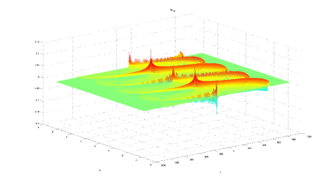
Figure 1: (Color online): $W_{RR}$ component of the Wigner function with initial conditions given as in (21), after 500 iterations.

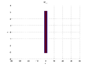
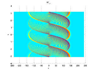
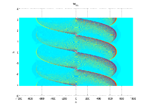
Figure 2: (Color online): Contour plots showing the time evolution of the $W_{RR}$ component of the Wigner function starting from the localized state (21). From left to right, the sub figures correspond to $t=0$, $t=100$ and $t=500$, respectively.

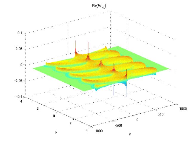
Figure 3: (Color online): Real part of the $W_{RL}$ component of the Wigner function with initial conditions given as in (21), after 500 iterations.

The momentum distribution is obtained from Eq. (17). We show in Fig. 4, as an example, the RR component of $M(k,t)$ plotted for $t=50,100,200$ and the same initial condition (21) as before. Since the moment $k$ is bounded, the distribution becomes more intricate as the QW evolves. At later times, the figure shows more oscillations, although the envelop remains constant, in accordance to the self-resemblance of the Wigner function as time increases.

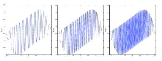
Figure 4: $M_{RR}(k,t)$ component with the same initial conditions as before, corresponding to times $t=50$, $t=100$ and $t=200$ (left to right).

For comparison, we investigate the Wigner function for a different initial condition. It corresponds to a “Schrödinger cat” in two positions $|\pm a\rangle$ which are entangled with two chiralities, i.e.:

$$\mid\psi(0)\rangle=\frac{1}{\sqrt{2}}(\mid a,R\rangle+i\mid-a,L\rangle).$$ (23)

The initial Wigner function for this state is now

$$W(n,k,0)=\frac{1}{2\pi}\left(\begin{array}[]{cc}\delta_{n,2a}&-ie^{-2ika}\delta_{n,0}\\ ie^{2ika}\delta_{n,0}&\delta_{n,-2a}\end{array}\right).$$ (24)

Notice that $a=0$ reproduces the localized state described above. The evolved component $W_{RR}$ of the Wigner function is shown in Fig. 5. Fig. 6 reveals the time evolution of this component. As compared to the previous case, it shows an even more complicated structure, thus suggesting a less classical state. This suggestion will be confirmed in the next section by comparing the negativity for both cases.

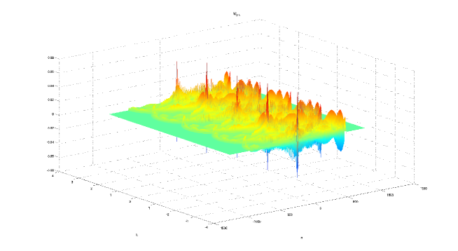
Figure 5: (Color online): $W_{RR}$ component of the Wigner function with initial conditions given as in (23), and $a=10$, after 500 iterations.

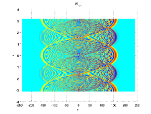
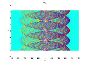
Figure 6: (Color online): Contour plots showing the time evolution of the $W_{RR}$ component of the Wigner function starting from the localized state (23) with $a=10$. From left to right, the sub figures correspond to $t=0$, $t=100$ and $t=500$.

V Negativity of the wigner function in the quantum walk

Consider the Wigner function, as defined in Eq. (4). As already mentioned, the fact that this function can take negative values implies that it cannot be considered as a classical probability distribution. Therefore, non positivity of the Wigner function can be interpreted as a measure of the non-classicality of the system. In quantum optics, this is interpreted as a signature for non-classical states of light, caused by a quantum interference phenomenon. In the context of finite dimensional systems, this idea is exploited in Franco and Penna (2006) to establish a criterion for entanglement in a system of two spin 1/2 particles. In Dahl et al. (2006), a connection is found between entanglement and the negativity of the Wigner function for hyperradial s-waves. Such states, in $D=2d$ dimensions, can be interpreted as the wave function of two entangled particles in $d$ dimensions.

A quantitative measure of non-classicality is given by the negativity, as defined in Kenfack and Zyczkowski (2004). In the continuous case, with variables $x$ and $p$, this volume can be written as:

$$\delta(W)=\int_{-\infty}^{\infty}\int_{-\infty}^{\infty}[\mid W(x,p)\mid-W(x,p)]dpdx=\int_{-\infty}^{\infty}\int_{-\infty}^{\infty}\mid W(x,p)\mid dpdx-1.$$ (25)

In deriving the latter equality, we made use of the fact that the total probability is normalized to one, so that $\int_{-\infty}^{\infty}\int_{-\infty}^{\infty}W(x,p)dpdx=1$. We will use $\delta(W)$, adopted to the discrete case, to compute the negativity of the Wigner function, and to explore whether we can relate the deviations from a classical behavior of the QW to the entanglement between the walker and the coin.

In our case, the Wigner function is a 2x2 matrix, and variables $x$, $p$ are to be replaced by $n$ and $k$, as defined in Sect. III. We propose, as a possible generalization of the above equation Banuls et al. (2012):

$$\delta(W)=\sum_{n}\int_{-\pi/2}^{\pi/2}[\mid\mid W(n,k)\mid\mid-Tr(W(n,k))]dk=\sum_{n}\int_{-\pi/2}^{\pi/2}\mid\mid W(n,k)\mid\mid dk-1,$$ (26)

and where we omitted the dependence on time to simplify the notation. Again, the latter equality arises as a consequence of normalization. As a measure of the norm $||A||$ of a matrix $A$, we adopt the trace norm, defined as:

$$\mid\mid A\mid\mid\equiv Tr\sqrt{A^{\dagger}A},$$ (27)

where $A^{\dagger}$ denotes the hermitian conjugate of $A$. If $\lambda_{1}(n,k)$, $\lambda_{2}(n,k)$ are the eigenvalues of $W(n,k)$ for a given $n$ and $k$, one obtains $||W||=\mid\lambda_{1}(n,k)\mid+\mid\lambda_{2}(n,k)\mid$. In this way, Eq. (26) adopts the following form:

$$\delta(W)=\int_{-\pi/2}^{\pi/2}\sum_{n}\left(\mid\lambda_{1}(n,k)\mid+\mid\lambda_{2}(n,k)\mid-\lambda_{1}(n,k)-\lambda_{2}(n,k)\right)dk,$$ (28)

which can be regarded as a natural generalization of (25).

We have numerically calculated the negativity (26) as a function of time, for the same initial conditions considered in the previous section: the localized state and two different cat states (Fig. 7).

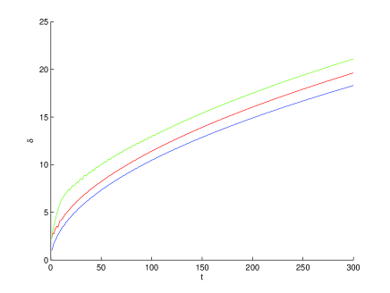
Figure 7: (Color online): Negativity, as a function of time, for the localized state $a=0$ (blue, bottom curve) and for the Schrödinger cat state with $a=4$ (red, middle curve) and $a=30$ (green, top curve).

We immediately observe that one obtains a higher degree of “quantumness” for the Schrödinger cat states, as compared to the localized state. This was expected from the higher degree of complexity observed in the Wigner function for the cat state, and implies a larger amount of interference effects. Higher values of the initial separation yield a larger negativity.

The question arises whether this higher degree of quantumness will also imply a higher entanglement between the walker and the coin. To this end, we use the entropy of entanglement as a quantity to characterize this property. To be more precise, we compute the quantity

$$S(t)=-Tr\{\rho_{c}(t)\log_{2}\rho_{c}(t)\},$$ (29)

where $\rho_{c}(t)=Tr_{S}\{\rho(t)\}$ is the density matrix for the coin, which is obtained by tracing out the spatial degrees of freedom.

Fig. 8 shows $S(t)$ for the localized state ($a=0$) and for the cat state with different values of the (half) separation $a$. The entanglement entropy is bounded by the (log of the) dimension of the coin space: $S(t)\leq 1$, and we can see that the time scale to reach this maximum is shorter for larger values of $a$, which also correspond to higher degrees of negativity, as seen in previous figures.

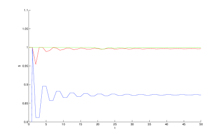
Figure 8: Entropy of the localized state $a=0$ (blue, bottom curve) and for the Schrödinger cat state with $a=4$ (red, middle curve) and $a=30$ (green, top curve).

VI Conclusions

In this paper, we have studied the discrete-time quantum walk on a one-dimensional lattice using the Wigner function. We have explored the potential of this phase-space representation to characterize the dynamics of the system. Differently to the case of a scalar wave function, we now have a $2\times 2$ matrix, defined over a phase space $(n,k)$. We have examined two cases, which correspond to different initial conditions. The first case starts with an initially localized state at $n=0$, as considered in many works in the literature. Its Wigner function shows a quite intricate structure, which is build up by interference effects on the lattice. We have also considered Schrödinger cat states, in which space and coin are initially entangled. It is apparent, from the Wigner function plots, that such states are capable of building up higher interference effects, and thus describe states that are even “less classical” than the previous one. In order to quantify this effect, we have computed the negativity associated to the Wigner function Kenfack and Zyczkowski (2004), as defined by the negative volume of the function in phase space. This definition has been extended to our case by the use of the trace norm of the Wigner matrix. As expected, the cat states give rise to a larger extent of negativity, which is even larger when the initial separation of the cat state is increased. In accordance to these ideas, one also obtains that the coin-walker entanglement evolves faster for the latter states. Altogether, the time evolution of the QW translates into an evolving state which separates from classicality. This separation, as time goes on, was expected from the fact that the walker distribution expands faster (with a quadratic deviation $\sigma\sim t$ ) than its classical counterpart (the random walk, for which $\sigma\sim\sqrt{t}$).