Abstract

In the problem of quantum state discrimination, one has to determine by measurements the state of a quantum system, based on the a priori side information that the true state is one of two given and completely known states, $\rho$ or $\sigma$. In general, it is not possible to decide the identity of the true state with certainty, and the optimal measurement strategy depends on whether the two possible errors (mistaking $\rho$ for $\sigma$, or the other way around) are treated as of equal importance or not. Results on the quantum Chernoff and Hoeffding bounds and the quantum Stein’s lemma show that, if several copies of the system are available then the optimal error probabilities decay exponentially in the number of copies, and the decay rate is given by a certain statistical distance between $\rho$ and $\sigma$ (the Chernoff distance, the Hoeffding distances, and the relative entropy, respectively). While these results provide a complete solution to the asymptotic problem, they are not completely satisfying from a practical point of view. Indeed, in realistic scenarios one has access only to finitely many copies of a system, and therefore it is desirable to have bounds on the error probabilities for finite sample size. In this paper we provide finite-size bounds on the so-called Stein errors, the Chernoff errors, the Hoeffding errors and the mixed error probabilities related to the Chernoff and the Hoeffding errors.

Keywords: State discrimination, Rényi relative entropies, Hoeffding distance, Chernoff distance, Neyman-Pearson tests, Holevo-Helström tests, Stein’s lemma.

1 Introduction

Assume we have a quantum system with a finite-dimensional Hilbert space ${\mathcal{H}}$, and we know that the system has been prepared either in state $\rho$ (this is our null hypothesis $H_{0}$) or state $\sigma$ (this is our alternative hypthesis $H_{1}$). (By a state we mean a density operator, i.e., a positive semi-definite operator with trace $1$). The goal of state discrimination is to come up with a “good” guess for the true state, based on measurements on the system. By “good” we mean that some error probability is minimal; we will specify this later. We will study the asymptotic scenario, where we assume that several identical and independent (i.i.d.) copies of the system are available, and we are allowed to make arbitrary collective measurements on the system. Due to the i.i.d. assumption, i.e., that the copies are identical and independent, the joint state of the $n$-copy system is either $\rho_{n}:=\rho^{\otimes n}$ or $\sigma_{n}:=\sigma^{\otimes n}$ for every $n\in\mathbb{N}$.

A test on $n$ copies is an operator $T\in{\mathcal{B}}({\mathcal{H}}^{\otimes n}),\,0\leq T\leq I_{n}$, that determines the binary POVM $(T,I_{n}-T)$. If the outcome corresponding to $T$ occurs then we accept the null hypothesis to be true, otherwise we accept the alternative hypothesis. Of course, we might make an error by concluding that the true state is $\sigma$ when it is actually $\rho$ (error of the first kind or type I error) or the other way around (error of the second kind or type II error). The probabilities of these errors when the measurement $(T,I_{n}-T)$ was performed are given by

$$\alpha_{n}(T):=\operatorname{Tr}\rho_{n}(I_{n}-T)\mbox{ }\mbox{ }\mbox{ }\mbox{ }\text{(first kind)\mbox{ }\mbox{ }\mbox{ }\mbox{ }and}\mbox{ }\mbox{ }\mbox{ }\mbox{ }\beta_{n}(T):=\operatorname{Tr}\sigma_{n}T\mbox{ }\mbox{ }\mbox{ }\mbox{ }\text{(second kind)}.$$

Unless $\rho_{n}$ and $\sigma_{n}$ are perfectly distinguishable (which is the case if and only if $\operatorname{supp}\rho_{n}\perp\operatorname{supp}\sigma_{n}$), the two error probabilities cannot be simultaneously eliminated, i.e., $\alpha_{n}(T)+\beta_{n}(T)>0$ for any test $T$, and our aim is to find a joint optimum of the two error probabilities, according to some criteria.

In a Bayesian approach, one considers the scenario where $\rho$ and $\sigma$ are prepared with some prior probabilities $p$ and $1-p$, respectively; the natural quantities to consider in this case are the so-called Chernoff errors, given by $\min_{T\text{ test}}\{p\alpha_{n}(T)+(1-p)\beta_{n}(T)\}$. More generally, consider for any $\kappa,\lambda>0$ the quantities

$$e_{n,\kappa,\lambda}:=\min_{T\text{ test}}\{\kappa\alpha_{n}(T)+\lambda\beta_{n}(T)\}.$$

For a self-adjoint operator $X$ and constant $c\in\mathbb{R}$, let $\{X>c\}$ denote the spectral projection of $X$ corresponding to the interval $(c,+\infty)$. We define $\{X\geq c\}$, $\{X<c\}$ and $\{X\leq c\}$ similarly. As one can easily see,

$$e_{n,\kappa,\lambda}=\frac{\kappa+\lambda}{2}-\frac{1}{2}\left\|\kappa\rho_{n}-\lambda\sigma_{n}\right\|_{1},$$

(where $\left\|X\right\|_{1}:=\operatorname{Tr}|X|$ for any operator $X$), and the minimum is reached at any test $T$ satisfying

$$\{\kappa\rho_{n}-\lambda\sigma_{n}>0\}\leq T\leq\{\kappa\rho_{n}-\lambda\sigma_{n}\geq 0\}.$$

Such a test is called a Neyman-Pearson test or Holevo-Helström test in the literature [17, 24]. By the above, such tests are optimal from the point of view of trade-off between the two error probabilities. Indeed, if $T$ is a Neyman-Pearson test corresponding to $\kappa$ and $\lambda$ then for any other test $S$ we have

$$\kappa\alpha_{n}(T)+\lambda\beta_{n}(T)\leq\kappa\alpha_{n}(S)+\lambda\beta_{n}(S).$$

In particular, if $\alpha_{n}(S)<\alpha_{n}(T)$ then necessarily $\beta_{n}(S)>\beta_{n}(T)$ and vice versa, i.e., if $S$ performs better than a Neymann-Pearson test for one of the error probabilities then it necessarily performs worse for the other. This is the so-called quantum Neyman-Pearson lemma. For later use, we introduce the notations

$$\mathcal{N}_{n,a}:=\{T\text{ test}\,:\,\{e^{-na}\rho_{n}-\sigma_{n}>0\}\leq T\leq\{e^{-na}\rho_{n}-\sigma_{n}\geq 0\}\}$$ (1)

and

$$e_{n}(a) :=e_{n,e^{-na},1}=\min_{T\text{ test}}\{e^{-na}\alpha_{n}(T)+\beta_{n}(T)\}$$

$$=e^{-na}\alpha_{n}(T)+\beta_{n}(T),\mbox{ }\mbox{ }T\in\mathcal{N}_{n,a},$$ (2)

where $a\in\mathbb{R}$ is a parameter.

The following has been shown for the i.i.d. case in [2, 32] (see also [20, 21, 22, 27, 28] for various generalizations to correlated settings).

Theorem 1.1.

For any $\kappa,\lambda>0$ we have

$$-\lim_{n\to\infty}\frac{1}{n}\log e_{n,\kappa,\lambda}=-\lim_{n\to\infty}\frac{1}{n}\log e_{n}(0)=C\left(\rho\,||\,\sigma\right):=-\inf_{0\leq t\leq 1}\log\operatorname{Tr}\rho^{t}\sigma^{1-t},$$

where $C\left(\rho\,||\,\sigma\right)$ is called the Chernoff distance of $\rho$ and $\sigma$.

Another natural way to optimize the two error probabilities is to put a constraint on one of them and optimize the other one under this constraint. It is usual to optimize the type II error under the constraint that the type I error is kept under a constant error bar $\varepsilon\in(0,1)$, in which case we are interested in the quantities

$$\beta_{n,\varepsilon}:=\min\{\beta_{n}(T)\,:\,T\text{ test, }\alpha_{n}(T)\leq\varepsilon\}.$$ (3)

Another natural choice is when an exponential constraint is imposed on the type I error, which gives

$$\beta_{n,e^{-nr}}:=\min\{\beta_{n}(T)\,:\,T\text{ test, }\alpha_{n}(T)\leq e^{-nr}\}$$ (4)

for some fixed parameter $r>0$. Unlike for the quantities $e_{n,\kappa,\lambda}$ above, there are no explicit expressions known for the values of $\beta_{n,\varepsilon}$ and $\beta_{n,e^{-nr}}$, or for the tests achieving them. However, the asymptotic behaviours are known also in these cases. The asymptotics of $\beta_{n,\varepsilon}$ is given by the quantum Stein’s lemma, first proved for the i.i.d. case in [18, 33] and later generalized to various correlated scenarios in [7, 8, 19, 21, 22, 27, 28].

Theorem 1.2.

We have

$$-\lim_{n\to+\infty}\frac{1}{n}\log\beta_{n,\varepsilon}=\inf_{\{T_{n}\}_{n\in\mathbb{N}}}\left\{-\lim_{n\to\infty}\frac{1}{n}\log\beta_{n}(T_{n})\,:\,\lim_{n\to\infty}\alpha_{n}(T_{n})=0\right\}=S\left(\rho\,||\,\sigma\right),$$

where the infimimum is taken over all sequences of measurements for which the indicated limit exists, and $S\left(\rho\,||\,\sigma\right)$ is the relative entropy of $\rho$ with respect to $\sigma$.

The asymptotics of $\beta_{n,e^{-nr}}$ has been an open problem for a long time (see, e.g., [15]), which was finally solved for the i.i.d. case in [16] and [30] (apart from some minor technicalities that were treated both in [3] and [21]), based on the techniques developed in [2] and [32]. These results were later extended to various correlated settings in [21, 22, 27, 28].

Theorem 1.3.

For any $r>0$ we have

$$-\lim_{n\to\infty}\frac{1}{n}\log\beta_{n,e^{-nr}}=H_{r}\left(\rho\,||\,\sigma\right):=-\inf_{0\leq t<1}\left\{\frac{tr+\log\operatorname{Tr}\rho^{t}\sigma^{1-t}}{1-t}\right\},$$

where $H_{r}\left(\rho\,||\,\sigma\right)$ is the Hoeffding distance of $\rho$ and $\sigma$ with parameter $r$.

It is not too difficult to see that Theorem 1.3 can also be reformulated in the following way:

$$H_{r}\left(\rho\,||\,\sigma\right)=\inf_{\{T_{n}\}_{n\in\mathbb{N}}}\left\{-\lim_{n\to\infty}\frac{1}{n}\log\beta_{n}(T_{n})\,:\,\limsup_{n\to\infty}\frac{1}{n}\log\alpha_{n}(T_{n})\leq-r\right\},$$

where the infimum is taken over all possible sequences of tests for which the indicated limit exists (see [21] for details). This formulation makes it clear that the Hoeffding distance quantifies the trade-off between the two error probabilities in the sense that it gives the optimal exponential decay of the error of the second kind under the constraint that the error of the first kind decays with a given exponential speed.

While there is no explicit expression known for the optimal tests minimizing (3) and (4), it is known that the Neyman-Pearson tests are asymptotically optimal for this problem in the sense given in Theorem 1.4 below. For a positive semidefinite operator $X$ and $x\in\mathbb{R}$, let $P_{x}$ denote the spectral projection of $X$ corresponding to the singleton $\{x\}$. For every $t\in\mathbb{R}$, we define $X^{t}:=\sum_{x>0}x^{t}P_{x}$; in particular, $X^{0}$ denotes the projection onto the support of $X$, i.e., $X^{0}=\{X>0\}$. The following was given in [21]:

Theorem 1.4.

For any $r>-\log\operatorname{Tr}\rho\sigma^{0}$, let $a_{r}:=H_{r}\left(\rho\,||\,\sigma\right)-r$. For any sequence of tests $\{T_{n}\}$ satisfying $T_{n}\in\mathcal{N}_{n,a_{r}},\,n\in\mathbb{N}$, we have

$$-\lim_{n\to\infty}\frac{1}{n}\log\alpha_{n}(T_{n}) =\hat{\varphi}(a_{r})=r,$$

$$-\lim_{n\to\infty}\frac{1}{n}\log\beta_{n}(T_{n}) =-\lim_{n\to\infty}\frac{1}{n}\log e_{n}(a_{r})=\varphi(a_{r})=H_{r}\left(\rho\,||\,\sigma\right),$$

where for every $a\in\mathbb{R}$,

$$\varphi(a):=\max_{0\leq t\leq 1}\{at-\log\operatorname{Tr}\rho^{t}\sigma^{1-t}\},\mbox{ }\mbox{ }\mbox{ }\mbox{ }\mbox{ }\mbox{ }\hat{\varphi}(a):=\varphi(a)-a.$$ (5)

Theorems 1.1–1.4 give a complete solution to the asymptotic problem in the most generally considered setups. These results, however, rely on the assumption that one has access to an unlimited number of identical copies of the system in consideration, which of course is never satisfied in reality. Note also that the above results give no information about the error probabilities for finite sample size, which is the relevant question from a practical point of view. Our aim in this paper is to provide bounds on the finite-size error probabilities that can be more useful for applications. There are two similar but slightly different ways to do so; one is to consider the optimal type II errors for finite $n$; we treat this in Section 3. The other is to study the asymptotic behaviour of the error probabilities corresponding to the Holevo-Helström measurements, that are known to be asymptotically optimal; we provide bounds on these error probabilities in Section 4. In the special case where both hypotheses are classical binary probability measures, a direct computation yields bounds on the mixed error probabilities $e_{n}(a)$; we present this in the Appendix. Some of the technical background is summarized in Section 2 below.

2 Preliminaries

2.1 Rényi relative entropies and related measures

For positive semidefinite operators $A,B$ on a Hilbert space ${\mathcal{K}}$, we define their Rényi relative entropy with parameter $t\in[0,+\infty)\setminus\{1\}$ as

$$S_{t}\left(A\,||\,B\right):=\begin{cases}\frac{1}{t-1}\log\operatorname{Tr}A^{t}B^{1-t}=\frac{1}{t-1}\psi_{A,B}\left(t\right),&\text{if}\mbox{ }\mbox{ }t\in[0,1)\mbox{ }\text{or}\mbox{ }\operatorname{supp}A\leq\operatorname{supp}B,\\ +\infty,&\text{otherwise},\end{cases}$$

where

$$\psi_{A,B}\left(t\right):=\log Z_{A,B}(t),\mbox{ }\mbox{ }\mbox{ }\mbox{ }\mbox{ }\mbox{ }Z_{A,B}(t):=\operatorname{Tr}A^{t}B^{1-t},\mbox{ }\mbox{ }\mbox{ }\mbox{ }\mbox{ }\mbox{ }t\in\mathbb{R}.$$

Here we use the convention $\log 0:=-\infty$ and $0^{t}:=0$, i.e., all powers are computed on the supports of $A$ and $B$, respectively. In particular, $S_{t}\left(A\,||\,B\right)=+\infty$ if and only if $\operatorname{supp}A\perp\operatorname{supp}B$ and $t\in[0,1)$, or $\operatorname{supp}A\nleq\operatorname{supp}B$ and $t>1$. Note that $Z_{A,B}(t)$ is a quasi-entropy in the sense of [34]. For most of what follows, we fix $A$ and $B$, and hence we omit them from the subscripts, i.e., we use $\psi$ instead of $\psi_{A,B}$, etc.

If $p$ is a positive measure on some finite set ${\mathcal{X}}$ then it can be naturally identified with a positive function, which we will denote the same way, i.e., we have the identity $p(\{x\})=p(x),\,x\in{\mathcal{X}}$. Moreover, $p$ can be naturally identified with a positive semidefinite operator on $\mathbb{C}^{{\mathcal{X}}}=l^{2}({\mathcal{X}})$, which we again denote the same way; the matrix of this operator is given by $\langle e_{x},pe_{y}\rangle=\delta_{x,y}p(x)$, where $\{e_{x}\}_{x\in{\mathcal{X}}}$ is the canonical basis of $\mathbb{C}^{{\mathcal{X}}}$. Given this identification, we can use the above definition to define the Rényi relative entropies of positive measures/functions $p$ and $q$ on some finite set ${\mathcal{X}}$, and we get $S_{t}\left(p\,||\,q\right)=\frac{1}{t-1}\log\sum_{x\in{\mathcal{X}}}p(x)^{t}q(x)^{1-t}$ whenever $S_{t}\left(p\,||\,q\right)$ is finite.

Let $A=\sum_{i\in\mathcal{I}}a_{i}P_{i}$ and $B=\sum_{j\in\mathcal{J}}b_{j}Q_{j}$ be decompositions of the positive semidefinite operators $A$ and $B$ such that $\{P_{i}\}$ and $\{Q_{j}\}$ are sets of orthogonal projections and $a_{i},b_{j}>0$ for all $i$ and $j$. Let ${\mathcal{X}}_{A,B}:=\{(i,j)\,:\,\operatorname{Tr}P_{i}Q_{j}>0\}$, and define

$$p_{A,B}(i,j):=a_{i}\operatorname{Tr}P_{i}Q_{j},\mbox{ }\mbox{ }\mbox{ }\mbox{ }\mbox{ }\mbox{ }q_{A,B}(i,j):=b_{j}\operatorname{Tr}P_{i}Q_{j},\mbox{ }\mbox{ }\mbox{ }\mbox{ }\mbox{ }\mbox{ }(i,j)\in{\mathcal{X}}_{A,B}.$$ (6)

Then $p=p_{A,B}$ and $q=q_{A,B}$ are positive measures on ${\mathcal{X}}={\mathcal{X}}_{A,B}$, and we have

$$\psi_{A,B}(t)=\psi_{p,q}(t),\mbox{ }\mbox{ }t\in\mathbb{R},\mbox{ }\mbox{ }\mbox{ }\mbox{ }\text{and}\mbox{ }\mbox{ }\mbox{ }\mbox{ }S_{t}\left(A\,||\,B\right)=S_{t}\left(p\,||\,q\right),\mbox{ }\mbox{ }t\in[0,1).$$

It is easy to see that

$$\operatorname{supp}p=\operatorname{supp}q={\mathcal{X}}\mbox{ }\mbox{ }\mbox{ }\mbox{ }\mbox{ }\mbox{ }\mbox{ }\mbox{ }\text{and}\mbox{ }\mbox{ }\mbox{ }\mbox{ }\mbox{ }\mbox{ }\mbox{ }\mbox{ }p({\mathcal{X}})=\operatorname{Tr}AB^{0},\mbox{ }\mbox{ }q({\mathcal{X}})=\operatorname{Tr}A^{0}B.$$

Note that the decompositions of $A$ and $B$ are not unique, and hence neither are the set ${\mathcal{X}}$ and the measures $p$ and $q$. However, if ${\mathcal{X}},p,q$ are defined through some decompositions $A=\sum_{i\in\mathcal{I}}a_{i}P_{i}$ and $B=\sum_{j\in\mathcal{J}}b_{j}Q_{j}$ then we will always assume that for every $n\in\mathbb{N}$, ${\mathcal{X}}_{A^{\otimes n},B^{\otimes n}},p_{A^{\otimes n},B^{\otimes n}}$ and $q_{A^{\otimes n},B^{\otimes n}}$ are defined through the decompositions $A^{\otimes n}=\sum_{\underline{i}\in\mathcal{I}^{n}}a_{\underline{i}}P_{\underline{i}}$ and $B=\sum_{\underline{j}\in\mathcal{J}^{n}}b_{\underline{j}}Q_{\underline{j}}$, where $a_{\underline{i}}:=a_{i_{1}}\cdot\ldots\cdot a_{i_{n}}$, $P_{\underline{i}}:=P_{i_{1}}\otimes\ldots\otimes P_{i_{n}}$, etc. In this way, we have

$${\mathcal{X}}_{A^{\otimes n},B^{\otimes n}}={\mathcal{X}}_{A,B}^{n},\mbox{ }\mbox{ }\mbox{ }\mbox{ }\mbox{ }\mbox{ }p_{A^{\otimes n},B^{\otimes n}}=p_{A,B}^{\otimes n},\mbox{ }\mbox{ }\mbox{ }\mbox{ }\mbox{ }\mbox{ }q_{A^{\otimes n},B^{\otimes n}}=q_{A,B}^{\otimes n}.$$

The above mapping of pairs of positive semi-definite operators to pairs of classical positive measures was used to prove the optimality of the quantum Chernoff bound in [32] and subsequently the optimality of the quantum Hoeffding bound in [30], by mapping the quantum state discrimination problem into a classical one. We will use the same approach to give lower bounds on the mixed error probabilities in Section 4.

For given $A,B$, and every $t\in\mathbb{R}$, define a probability measure $\mu^{t}$ on ${\mathcal{X}}$ as

$$\mu^{t}(i,j):=\frac{1}{Z(t)}p(i,j)^{t}q(i,j)^{1-t},\mbox{ }\mbox{ }\mbox{ }\mbox{ }\mbox{ }\mbox{ }(i,j)\in{\mathcal{X}},$$

where ${\mathcal{X}},p,q$ are given as above, and $Z(t)=Z_{A,B}(t)=\sum_{i,j}p(i,j)^{t}q(i,j)^{1-t},\,t\in\mathbb{R}$.

Lemma 2.1.

The function $\psi$ is convex on $\mathbb{R}$, it is affine if and only if $q$ is a constant multiple of $p$ and otherwise $\psi^{\prime\prime}(t)>0$ for all $t\in\mathbb{R}$.

Proof.

A straightforward computation shows that

$$\psi^{\prime}(t) =Z(t)^{-1}\sum_{i,j}p(i,j)^{t}q(i,j)^{1-t}(\log p(i,j)-\log q(i,j))=\operatorname{\mathbb{E}}_{\mu^{t}}f,$$ (7)

$$\psi^{\prime\prime}(t) =\operatorname{\mathbb{E}}_{\mu^{t}}(f)^{2}-(\operatorname{\mathbb{E}}_{\mu^{t}}f)^{2}$$

$$=\frac{\operatorname{Tr}A^{t}B^{1-t}(\log A-\log B)^{2}}{\operatorname{Tr}A^{t}B^{1-t}}-\left(\frac{\operatorname{Tr}A^{t}B^{1-t}(\log A-\log B)}{\operatorname{Tr}A^{t}B^{1-t}}\right)^{2},$$ (8)

where $f(i,j):=\log p(i,j)-\log q(i,j),\,(i,j)\in{\mathcal{X}}$, and $\operatorname{\mathbb{E}}_{\mu^{t}}$ denotes the expectation value with respect to $\mu^{t}$. This shows that $\psi$ is convex on the whole real line, and $\psi^{\prime\prime}(t)=0$ for some $t\in\mathbb{R}$ if and only if $f$ is constant, which is equivalent to $q$ being a constant multiple of $p$. Since this condition for a flat second derivative is independent of $t$, the assertion follows. ∎

For a condition for a flat derivative of $\psi$ in terms of $A$ and $B$, see Lemma 3.2 in [21].

Corollary 2.2.

If $\operatorname{Tr}A\leq 1$ then the function $t\mapsto S_{t}\left(A\,||\,B\right)$ is monotone increasing on $[0,1)$ and on $(1,+\infty)$. If $\operatorname{Tr}A=1$ then we have

$$\lim_{t\to 1}S_{t}\left(A\,||\,B\right)=S_{1}\left(A\,||\,B\right):=S\left(A\,||\,B\right):=\begin{cases}\operatorname{Tr}A(\log^{*}A-\log^{*}B),&\operatorname{supp}A\leq\operatorname{supp}B,\\ +\infty,&\text{otherwise},\end{cases}$$

where $\log^{*}x=\log x,\,x>0$, and $\log^{*}0:=0$.

Proof.

We have $\frac{d}{dt}S_{t}\left(A\,||\,B\right)=\frac{\psi^{\prime}(t)(t-1)-\psi(t)}{(t-1)^{2}}=\frac{-\psi(1)}{(t-1)^{2}}+\frac{1}{2}\psi^{\prime\prime}(\xi_{t})$, where $\xi_{t}$ is between $t$ and $1$. The first assertion then follows due to Lemma 2.1. If $\operatorname{Tr}A=1$ then $\lim_{t\to 1}S_{t}\left(A\,||\,B\right)=\psi^{\prime}(1)$, which is easily seen to be equal to $S\left(A\,||\,B\right)$. ∎

The quantity $S\left(A\,||\,B\right)$ defined above is the relative entropy of $A$ with respect to $B$. The following Lemma complements Corollary 2.2:

Lemma 2.3.

Assume that $\operatorname{supp}A\leq\operatorname{supp}B$. For any $c>0$ and $|t-1|\leq\delta:=\min\left\{\frac{1}{2},\frac{c}{2\log\eta}\right\}$, where

$$\eta:=1+e^{\frac{1}{2}S_{3/2}\left(A\,||\,B\right)}+e^{-\frac{1}{2}S_{1/2}\left(A\,||\,B\right)},$$ (9)

we have

$$S_{t}\left(A\,||\,B\right) \geq S\left(A\,||\,B\right)-(4\cosh c)(1-t)(\log\eta)^{2},\mbox{ }\mbox{ }\mbox{ }\mbox{ }t\in(1-\delta,1),$$ (10)

$$S_{t}\left(A\,||\,B\right) \leq S\left(A\,||\,B\right)+(4\cosh c)(t-1)(\log\eta)^{2},\mbox{ }\mbox{ }\mbox{ }\mbox{ }t\in(1,1+\delta).$$ (11)

With the convention $S_{1}\left(A\,||\,B\right):=S\left(A\,||\,B\right)$, the above inequalities can be combined into

$$S_{\beta}\left(A\,||\,B\right) \leq S_{t}\left(A\,||\,B\right)+(4\cosh c)(\log\eta)^{2}(\beta-t),\mbox{ }\mbox{ }\mbox{ }\mbox{ }1-\delta\leq t\leq 1\leq\beta\leq 1+\delta.$$

Proof.

The inequality (11) was first given for conditional entropies in [37] and for relative entropies of states in [38]. Exactly the same proof yields (11) for general positive semidefinite operators, and also the inequality (10). ∎

For an operator $X$ on a finite-dimensional Hilbert space, let $\left\|X\right\|_{1}:=\operatorname{Tr}|X|=\operatorname{Tr}\sqrt{X^{*}X}$ denote its trace-norm. The von Neumann entropy of a positive semi-definite operator $A$ is defined as $S(A):=-\operatorname{Tr}A\log A=-S\left(A\,||\,I\right)$. The following is a sharpening of the Fannes inequality [13]; for a proof, see, e.g., [1] or [35].

Lemma 2.4.

For density operators $A$ and $B$ on a finite-dimensional Hilbert space ${\mathcal{H}}$,

$$|S(A)-S(B)|\leq\frac{1}{2}\left\|A-B\right\|_{1}\log(\dim{\mathcal{H}}-1)+h_{2}(\left\|A-B\right\|_{1}/2),$$

where $h_{2}(x):=-x\log x-(1-x)\log(1-x),\,x\in[0,1]$.

For positive semidefinite operators $A$ and $B$, we define their Chernoff distance as

$$C\left(A\,||\,B\right):=-\min_{0\leq t\leq 1}\log\operatorname{Tr}A^{t}B^{1-t}=\sup_{0\leq t<1}\left\{(1-t)S_{t}\left(A\,||\,B\right)\right\}.$$

The following inequality between the trace-norm and the Chernoff distance was given in Theorem 1 of [2]; see also the simplified proof by N. Ozawa in [25].

Lemma 2.5.

Let $A$ and $B$ be positive semidefinite operators on a finite-dimensional Hilbert space ${\mathcal{H}}$. Then

$$\frac{1}{2}\operatorname{Tr}(A+B)-\frac{1}{2}\operatorname{Tr}|A-B|\leq\operatorname{Tr}A^{t}B^{1-t},\mbox{ }\mbox{ }\mbox{ }\mbox{ }\mbox{ }\mbox{ }t\in[0,1],$$

or equivalently,

$$\frac{1}{2}\operatorname{Tr}(A+B)-\frac{1}{2}\left\|A-B\right\|_{1}\leq e^{-C\left(A\,||\,B\right)}.$$

The above lemma was used to prove the achievability of the quantum Chernoff bound in [2], and subsequently the achievability of the quantum Hoeffding bound in [16]. We will recall these results in Section 4.

The Hoeffding distance of $A$ and $B$ with parameter $r\geq 0$ is defined as

$$H_{r}\left(A\,||\,B\right):=\sup_{0\leq t<1}\left\{S_{t}\left(A\,||\,B\right)-\frac{tr}{1-t}\right\}=\sup_{0\leq t<1}\frac{-tr-\log\operatorname{Tr}A^{t}B^{1-t}}{1-t}$$

(cf. Theorem 1.3 for the same expression for density operators). For every $a\in\mathbb{R}$, let

$$\varphi(a):=\max_{t\in[0,1]}\{ta-\psi(t)\},\mbox{ }\mbox{ }\mbox{ }\mbox{ }\mbox{ }\mbox{ }\hat{\varphi}(a):=\max_{t\in[0,1]}\{(t-1)a-\psi(t)\}=\varphi(a)-a.$$

as in (5).

Lemma 2.6.

1. The function $r\mapsto H_{r}\left(A\,||\,B\right)$ is convex and monotonic decreasing.

2. $\lim_{r\searrow 0}H_{r}\left(A\,||\,B\right)=H_{0}\left(A\,||\,B\right)$, and if $\operatorname{Tr}A=1$ then $H_{0}\left(A\,||\,B\right)=S\left(A\,||\,B\right)$.

3. For every $-\psi(1)<r<-\psi(0)-\psi^{\prime}(0)$ there exists a unique $t_{r}\in(0,1)$ such that

   $$r=S\left(\mu^{t_{r}}\,||\,p\right)=(t_{r}-1)\psi^{\prime}(t_{r})-\psi(t_{r}),\mbox{ }\mbox{ }\mbox{ }\mbox{ }\mbox{ }\mbox{ }H_{r}\left(A\,||\,B\right)=S\left(\mu^{t_{r}}\,||\,q\right)=t_{r}\psi^{\prime}(t_{r})-\psi(t_{r}).$$

4. For every $r>-\psi(1)$ there is a unique $a_{r}\in\mathbb{R}$ such that

   $$\varphi(a_{r})=H_{r}\left(A\,||\,B\right),\mbox{ }\mbox{ }\mbox{ }\mbox{ }\mbox{ }\mbox{ }\mbox{ }\mbox{ }\mbox{ }\mbox{ }\hat{\varphi}(a_{r})=r.$$ (12)

   Moreover, $a_{r}=H_{r}\left(A\,||\,B\right)-r$, and if $r<-\psi(0)-\psi^{\prime}(0)$ then $a_{r}=\psi^{\prime}(t_{r})$ with the $t_{r}$ given in (iii).

Proof.

The first assertion is obvious from the definition, and the second identity in (ii) follows immediately from Corollary 2.2. Note that

$$H_{r}\left(A\,||\,B\right)=\sup_{0\leq t<1}\frac{-tr-\psi(t)}{1-t}=\sup_{s\geq 0}\{-sr-\tilde{\psi}(s)\},$$

where $\tilde{\psi}(s):=(1+s)\psi\left(\frac{s}{1+s}\right)$, and hence the function $r\mapsto H_{r}\left(A\,||\,B\right)$ is essentially the Legendre transform of $\tilde{\psi}$. By Proposition 4.1 and Corollary 4.1 in [12], $\tilde{\psi}^{*}$ is lower semicontinuous, and hence $\liminf_{r\searrow 0}H_{r}\left(A\,||\,B\right)\geq H_{0}\left(A\,||\,B\right)\geq\lim_{r\searrow 0}H_{r}\left(A\,||\,B\right)$, where the second inequality is due to the monotonicity in $r$. This gives the first identity in (ii).

Convexity of $\psi$ yields that $\psi(0)+\psi^{\prime}(0)\leq\psi(1)$ and equality holds if and only if $\psi$ is affine, in which case the assertion in (iii) is empty and hence for the rest we assume $\psi^{\prime\prime}(t)>0,\,t\in\mathbb{R}$. By the definition of $\tilde{\psi}$,

$$\tilde{\psi}^{\prime}(s)=\psi\left(\frac{s}{1+s}\right)+\frac{1}{1+s}\psi^{\prime}\left(\frac{s}{1+s}\right)\mbox{ }\mbox{ }\mbox{ }\mbox{ }\text{and}\mbox{ }\mbox{ }\mbox{ }\mbox{ }\tilde{\psi}^{\prime\prime}(s)=\frac{1}{(1+s)^{3}}\psi^{\prime\prime}\left(\frac{s}{1+s}\right),$$

and hence $\tilde{\psi}$ is also convex. Note that $\tilde{\psi}^{\prime}(0)=\psi(0)+\psi^{\prime}(0)$ and $\lim_{s\to+\infty}\tilde{\psi}^{\prime}(s)=\psi(1)$, and hence,

$$H_{r}\left(A\,||\,B\right)=\sup_{s\geq 0}\{-sr-\tilde{\psi}(s)\}=\begin{cases}-\tilde{\psi}(0)=-\psi(0),&-r\leq\psi(0)+\psi^{\prime}(0),\\ +\infty&-r>\psi(1).\end{cases}$$

On the other hand, for any $-\psi(1)<r<-\psi(0)-\psi^{\prime}(0)$ there exists a unique $s_{r}>0$ such that

$$-r=\tilde{\psi}^{\prime}(s_{r})=\psi(t_{r})+(1-t_{r})\psi^{\prime}(t_{r})\mbox{ }\mbox{ }\mbox{ }\mbox{ }\text{and}\mbox{ }\mbox{ }\mbox{ }\mbox{ }H_{r}\left(A\,||\,B\right)=-s_{r}r-\tilde{\psi}(s_{r})=-\psi(t_{r})+t_{r}\psi^{\prime}(t_{r}),$$

where $t_{r}=\frac{s_{r}}{1+s_{r}}\in(0,1)$. The identities

$$S\left(\mu^{t}\,||\,p\right)=(t-1)\psi^{\prime}(t)-\psi(t),\mbox{ }\mbox{ }\mbox{ }\mbox{ }\mbox{ }\mbox{ }S\left(\mu^{t}\,||\,q\right)=t\psi^{\prime}(t)-\psi(t),\mbox{ }\mbox{ }\mbox{ }\mbox{ }\mbox{ }\mbox{ }t\in\mathbb{R},$$

follow by a straightforward computation. This proves (iii). For $-\psi(1)<r<-\psi(0)-\psi^{\prime}(0)$, (iv) is an immediate consequence of (iii). For the general case, see e.g., Theorem 4.8 in [21]. ∎

Remark 2.7.

The equation of the tangent line of $\psi$ at point $t$ is $l(x):=\psi(t)+(x-t)\psi^{\prime}(t)$. Hence, $\psi(t)-t\psi^{\prime}(t)=-S\left(\mu^{t}\,||\,q\right)$ is its intersection with the $y$ axis and $\psi(t)-(t-1)\psi^{\prime}(t)=-S\left(\mu^{t}\,||\,p\right)$ is its intersection with the $x=1$ line.

Remark 2.8.

Note that

$$\psi(0) =\log\operatorname{Tr}A^{0}B=\log q({\mathcal{X}}),\mbox{ }\mbox{ }\text{and if}\mbox{ }\mbox{ }A^{0}\geq B^{0}\mbox{ }\mbox{ }\text{then}\mbox{ }\mbox{ }\psi^{\prime}(0)=-S\left(B\,||\,A\right)/\operatorname{Tr}B,$$

$$\psi(1) =\log\operatorname{Tr}AB^{0}=\log p({\mathcal{X}}),\mbox{ }\mbox{ }\text{and if}\mbox{ }\mbox{ }A^{0}\leq B^{0}\mbox{ }\mbox{ }\text{then}\mbox{ }\mbox{ }\psi^{\prime}(1)=S\left(A\,||\,B\right)/\operatorname{Tr}A.$$

Remark 2.9.

It was shown in [23] that

$$H_{r}\left(p\,||\,q\right)=\inf\{S\left(\mu\,||\,q\right)\,:\,S\left(\mu\,||\,p\right)\leq r\},$$

where $p$ and $q$ are probability distributions on some finite set ${\mathcal{X}}$, and $\mu^{t_{r}}$ with the $t_{r}$ given in Lemma 2.6 is a unique minimizer in the above expression. However, the above representation of the Hoeffding distance does not hold in the quantum case. Indeed, it was shown in [15, 33] that for density operators $\rho$ and $\sigma$,

$$\inf\{S\left(\tilde{\rho}\,||\,\sigma\right)\,:\,\tilde{\rho}\text{ is a density operator, }S\left(\tilde{\rho}\,||\,\rho\right)\leq r\} =\sup_{0\leq t<1}\frac{-tr-\log\operatorname{Tr}e^{t\rho+(1-t)\sigma}}{1-t}$$

$$\geq H_{r}\left(\rho\,||\,\sigma\right),$$

where the inequality is due to the Golden-Thompson inequality (see, e.g., Theorem IX.3.7 in [6]), and is in general strict.

Although the Chernoff distance and the Hoeffding distances don’t satisfy the axioms of a metric on the set of density operators (the Chernoff distance is symmetric but does not satisfy the triangle inequality, while the Hoeffding distances are not even symmetric), the Lemma below gives some motivation why they are called “distances”.

Lemma 2.10.

If $\operatorname{Tr}A\leq 1$ and $\operatorname{Tr}B\leq 1$ then

$$S_{t}\left(A\,||\,B\right)\geq 0,\mbox{ }\mbox{ }\mbox{ }\mbox{ }\mbox{ }\mbox{ }C\left(A\,||\,B\right)\geq 0,\mbox{ }\mbox{ }\mbox{ }\mbox{ }\mbox{ }\mbox{ }H_{r}\left(A\,||\,B\right)\geq 0$$

for every $t\in(0,+\infty)\setminus\{1\}$ and every $r\geq 0$. Moreover, the above inequalities are strict unless $A=B$ and $\operatorname{Tr}A=1$ or $r>-\psi(0)-\psi^{\prime}(0)$.

Proof.

Hölder’s inequality (see Corollary IV.2.6 in [6]) yields that $\operatorname{Tr}A^{t}B^{1-t}\leq(\operatorname{Tr}A)^{t}(\operatorname{Tr}B)^{1-t}$ for every $t\in[0,1]$, from which the assertions follow easily, taking into account the previous Lemmas. ∎

2.2 Types

Let ${\mathcal{X}}$ be a finite set and let $\mathcal{M}({\mathcal{X}})$ denote the set of non-zero positive measures on ${\mathcal{X}}$ and $\mathcal{M}_{1}({\mathcal{X}})$ the set of probability measures on ${\mathcal{X}}$. We will identify positive measures with positive semidefinite operators as described in the previous subsection. For $\mu\in\mathcal{M}({\mathcal{X}})$ let $S(\mu):=-\sum_{x\in{\mathcal{X}}}\mu(x)\log\mu(x)$ be its entropy, and for $\mu_{1},\mu_{2}\in\mathcal{M}({\mathcal{X}})$ let the relative entropy of $\mu_{1}$ and $\mu_{2}$ be defined as $S\left(\mu_{1}\,||\,\mu_{2}\right):=\sum_{x\in{\mathcal{X}}}\mu_{1}(x)\log\frac{\mu_{1}(x)}{\mu_{2}(x)}$ if $\operatorname{supp}\mu_{1}\leq\operatorname{supp}\mu_{2}$, and $+\infty$ otherwise.

For a sequence $\underline{x}\in{\mathcal{X}}^{n}$, the type of $\underline{x}$ is the probability distribution given by

$$T_{\underline{x}}(y):=\frac{1}{n}|\{k\,:x_{k}=y\}|,\mbox{ }\mbox{ }\mbox{ }\mbox{ }\mbox{ }\mbox{ }y\in{\mathcal{X}},$$

where $|H|$ denotes the cardinality of a set $H$. Note that $T_{\underline{x}}=T_{\underline{y}}$ if and only if $\underline{x}$ is a permutation of $\underline{y}$. Obviously, if $\mu\in\mathcal{M}({\mathcal{X}})$ then the measure of an $\underline{x}\in{\mathcal{X}}^{n}$ with respect to $\mu^{\otimes n}$ only depends on the type of $\underline{x}$, and one can easily see that

$$\mu^{\otimes n}(\underline{x})=e^{-n\left(S\left(T_{\underline{x}}\,||\,\mu\right)+S(T_{\underline{x}})\right)}.$$

In particular,

$$T_{\underline{x}}^{\otimes n}(\underline{x})=e^{-nS(T_{\underline{x}})},\mbox{ }\mbox{ }\mbox{ }\mbox{ }\text{and}\mbox{ }\mbox{ }\mbox{ }\mbox{ }\mu^{\otimes n}(\underline{x})=T_{\underline{x}}^{\otimes n}(\underline{x})e^{-n\left(S\left(T_{\underline{x}}\,||\,\mu\right)\right)}.$$ (13)

A variant of the following bound can be found in [23]. For readers’ convenience we provide a complete proof here.

Lemma 2.11.

Let $\underline{x}\in{\mathcal{X}}^{n}$ and $r:=|\operatorname{supp}T_{\underline{x}}|$. Then,

$$\frac{1}{n}\log T_{\underline{x}}^{\otimes n}\left(\{\underline{y}\,:\,T_{\underline{y}}=T_{\underline{x}}\}\right)\geq-\frac{r-1}{2}\frac{\log n}{n}+\frac{r}{n}\left(\log(\sqrt{r/2\pi})-1/12\right)+\frac{1}{n(12n+1)}.$$

Proof.

Let $z_{1},\ldots,z_{r}$, be an ordering of the elements of $\operatorname{supp}T_{\underline{x}}$, and let $k_{i}:=nT_{\underline{x}}(z_{i})$. Then

$$|\{\underline{y}\,:\,T_{\underline{y}}=T_{\underline{x}}\}|=\frac{n!}{k_{1}!\cdot\ldots\cdot k_{r}!},\mbox{ }\mbox{ }\mbox{ }\mbox{ }\mbox{ }\mbox{ }\mbox{ }\mbox{ }T_{\underline{x}}^{\otimes n}(\underline{y})=\prod_{i=1}^{r}(k_{i}/n)^{k_{i}},\mbox{ }\mbox{ }T_{\underline{y}}=T_{\underline{x}}.$$

By Stirling’s formula (see, e.g., [14]),

$$(m/e)^{m}\sqrt{2\pi m}\,e^{1/(12m+1)}\leq m!\leq(m/e)^{m}\sqrt{2\pi m}\,e^{1/12m},$$

and hence,

$$p_{n} :=T_{\underline{x}}^{\otimes n}\left(\{\underline{y}\,:\,T_{\underline{y}}=T_{\underline{x}}\}\right)=|\{\underline{y}\,:\,T_{\underline{y}}=T_{\underline{x}}\}|T_{\underline{x}}^{\otimes n}(\underline{x})=\frac{n!}{n^{n}}\prod_{i=1}^{r}\frac{k_{i}^{k_{i}}}{k_{i}!}$$

$$\geq e^{-n}\,\sqrt{2\pi n}\,e^{1/(12n+1)}\prod_{i=1}^{r}e^{k_{i}}\sqrt{2\pi k_{i}}^{-1}e^{-1/12k_{i}}$$

$$=\frac{\sqrt{2\pi n}}{\sqrt{2\pi}^{r}\sqrt{k_{1}\cdot\ldots\cdot k_{r}}}\exp(1/(12n+1)-1/12k_{1}-\ldots-1/12k_{r}).$$

Using $\sqrt[r]{k_{1}\cdot\ldots\cdot k_{r}}\leq\frac{k_{1}+\ldots+k_{r}}{r}=\frac{n}{r}$, we have $\sqrt{k_{1}\cdot\ldots\cdot k_{r}}\leq(n/r)^{r/2}$, while $k_{i}\geq 1$ yields $1/k_{1}+\ldots+1/k_{r}\leq r$, and hence,

$$p_{n} \geq\frac{\sqrt{2\pi n}}{\sqrt{2\pi}^{r}}(r/n)^{r/2}\exp\left(\frac{1}{12n+1}-\frac{r}{12}\right)\geq(\sqrt{r/2\pi})^{r}n^{1/2-r/2}\exp\left(\frac{1}{12n+1}-\frac{r}{12}\right),$$

which yields

$$\frac{1}{n}\log p_{n}\geq-\frac{r-1}{2}\frac{\log n}{n}+\frac{r}{n}\left(\log(\sqrt{r/2\pi})-1/12\right)+\frac{1}{n(12n+1)}.\qed$$

Let $\mathcal{T}_{n}$ denote the collection of all types arising from length $n$ sequences, i.e., $\mathcal{T}_{n}:=\{T_{\underline{x}}\,:\,\underline{x}\in{\mathcal{X}}^{n}\}$. It is known that $\cup_{n\in\mathbb{N}}\mathcal{T}_{n}$ is dense in $\mathcal{M}_{1}({\mathcal{X}})$, and $\inf_{\nu\in\mathcal{T}_{n}}\left\|\mu-\nu\right\|_{1}\leq\frac{|{\mathcal{X}}|}{n}$ for any $\mu\in\mathcal{M}_{1}({\mathcal{X}})$; see, e.g., [11]. Moreover, the following has been shown in Lemma A.2 of [23]:

Lemma 2.12.

Let $v\in\mathbb{R}^{{\mathcal{X}}}$ and $c\in\mathbb{R}$, and assume that the half-spaces $H_{1}:=\{f\in\mathbb{R}^{{\mathcal{X}}}\,:\,\sum_{x\in{\mathcal{X}}}f(x)v(x)<c\}$ and $H_{2}:=\{f\in\mathbb{R}^{{\mathcal{X}}}\,:\,\sum_{x\in{\mathcal{X}}}f(x)v(x)>c\}$ have non-trivial intersections with $\mathcal{M}_{1}({\mathcal{X}})$. Then for every $\mu\in\mathcal{M}_{1}({\mathcal{X}})$ such that $\sum_{x\in{\mathcal{X}}}\mu(x)v(x)=c$, and every $n\geq r(r-1)$, where $r:=|\operatorname{supp}\mu|$, there exist types $\mu_{1}\in H_{1}\cap\mathcal{T}_{n}$ and $\mu_{2}\in H_{2}\cap\mathcal{T}_{n}$ such that

$$\max\left\{\left\|\mu-\mu_{1}\right\|_{1},\left\|\mu-\mu_{2}\right\|_{1}\right\}\leq\frac{2(r-1)}{n}.$$

For more about types and their applications in information theory, see e.g., [10].

3 Optimal Type II errors

Consider the state discrimination problem described in the Introduction. In this section, we will give bounds on the error probabilities $\beta_{n,\varepsilon}$ and $\beta_{n,e^{-nr}}$. The key technical tool will be the following lemma about the duality of linear programming, known as Slater’s condition; for a proof, see Problem 4 in Section 7.2 of [5].

Lemma 3.1.

Let $V_{1}$ and $V_{2}$ be real inner product spaces and let $K_{i}$ be a convex cone in $V_{i}$. The dual cone $K_{i}^{*}$ is defined as $K_{i}^{*}:=\{y\in V_{i}\,:\,\langle y,x\rangle\geq 0,\,x\in K_{i}\}$. Let $c\in V_{1},\,b\in V_{2}$ and let $A:\,V_{1}\to V_{2}$ be a linear map. Assume that there exists a $v$ in the interior of $K_{1}$ such that $Av-b$ is in the interior of $K_{2}$. Then the following two quantities are equal:

$$\gamma^{p}: =\inf\{\langle c,v\rangle\,:\,v\geq_{K_{1}}0,\,Av\geq_{K_{2}}b\},$$

$$\gamma^{d}: =\sup\{\langle b,w\rangle\,:\,w\geq_{K_{2}^{*}}0,\,A^{*}w\leq_{K_{1}^{*}}c\}.$$

Using Lemma 3.1, we can give the following alternative characterization of the optimal type II error:

Proposition 3.2.

For every $\varepsilon\in(0,1)$, we have

$$\beta_{1,\varepsilon} =\sup_{\lambda\geq 0}\{(1-\varepsilon)\lambda-\operatorname{Tr}(\lambda\rho-\sigma)_{+}\}=\sup_{\lambda\geq 0}\left\{\frac{\lambda+1}{2}-\frac{1}{2}\left\|\lambda\rho-\sigma\right\|_{1}-\lambda\varepsilon\right\}$$ (14)

$$\leq\sup_{\lambda\geq 0}\{\lambda^{t}\operatorname{Tr}\rho^{t}\sigma^{1-t}-\lambda\varepsilon\},\mbox{ }\mbox{ }\mbox{ }\mbox{ }\mbox{ }\mbox{ }t\in[0,1].$$ (15)

Moreover, for every $n\in\mathbb{N}$ and every $t\in[0,1)$,

$$\frac{1}{n}\log\beta_{n,\varepsilon}\leq-S_{t}\left(\rho\,||\,\sigma\right)+\frac{\log\varepsilon^{-1}}{n}\frac{t}{1-t}-\frac{1}{n}\frac{h_{2}(t)}{1-t},$$ (16)

where $h_{2}(t):=-t\log t-(1-t)\log(1-t),\,t\in[0,1]$.

Proof.

Let $\tilde{\rho}$ and $\tilde{\sigma}$ be density operators on some finite-dimensional Hilbert space, and for each $\varepsilon>0$ define

$$\beta_{\varepsilon}:=\min\{\operatorname{Tr}\tilde{\sigma}T\,:\,0\leq T\leq I,\,\operatorname{Tr}\tilde{\rho}(I-T)\leq\varepsilon\},$$

which is the optimal type II error for discriminating between $\tilde{\rho}$ and $\tilde{\sigma}$ under the constraint that the type I error doesn’t exceed $\varepsilon$. We apply Lemma 3.1 to give an alternative expression for $\beta_{\varepsilon}$. To this end, we define

$$V_{1}:={\mathcal{B}}({\mathcal{H}})_{sa},\mbox{ }\mbox{ }\mbox{ }\mbox{ }c:=\tilde{\sigma},\mbox{ }\mbox{ }\mbox{ }\mbox{ }\mbox{ }\mbox{ }V_{2}:={\mathcal{B}}({\mathcal{H}})_{sa}\oplus\mathbb{R},\mbox{ }\mbox{ }\mbox{ }\mbox{ }b:=-I\oplus(1-\varepsilon),$$

where ${\mathcal{B}}({\mathcal{H}})_{sa}$ is the real linear vector space of self-adjoint operators on ${\mathcal{H}}$. We equip both $V_{1}$ and $V_{2}$ with the Hilbert-Schmidt inner product, and define $K_{1}$ and $K_{2}$ to be the self-dual cones of the positive semidefinite operators. If we define $A$ to be $A:\,X\mapsto-X\oplus\operatorname{Tr}\tilde{\rho}X$ then $A^{*}$ is given by $A^{*}:\,X\oplus\lambda\mapsto-X+\lambda\tilde{\rho}$, and we see that $\gamma^{p}=\beta_{\varepsilon}$. It is easy to verify that the condition of Lemma 3.1 is satisfied in this case, and hence

$$\beta_{\varepsilon}=\gamma^{p}=\gamma^{d}=\sup\{-\operatorname{Tr}X+\lambda(1-\varepsilon)\,:\,X\geq 0,\,\lambda\geq 0,\,-X+\lambda\tilde{\rho}\leq\tilde{\sigma}\}.$$

For a fixed $\lambda\geq 0$, we have

$$\inf\{\operatorname{Tr}X\,:\,X\geq 0,\,\lambda\tilde{\rho}-\tilde{\sigma}\leq X\}=\operatorname{Tr}(\lambda\tilde{\rho}-\tilde{\sigma})_{+}=\frac{1}{2}\operatorname{Tr}(\lambda\tilde{\rho}-\tilde{\sigma})+\frac{1}{2}\left\|\lambda\tilde{\rho}-\tilde{\sigma}\right\|_{1}=\frac{\lambda-1}{2}+\frac{1}{2}\left\|\lambda\tilde{\rho}-\tilde{\sigma}\right\|_{1}$$

(the first identity can also be seen by a duality argument). Hence, we have

$$\beta_{\varepsilon} =\gamma^{d}=\sup_{\lambda\geq 0}\{(1-\varepsilon)\lambda-\operatorname{Tr}(\lambda\tilde{\rho}-\tilde{\sigma})_{+}\}=\sup_{\lambda\geq 0}\left\{\frac{\lambda+1}{2}-\frac{1}{2}\left\|\lambda\tilde{\rho}-\tilde{\sigma}\right\|_{1}-\lambda\varepsilon\right\}$$

$$\leq\sup_{\lambda\geq 0}\{\lambda^{t}\operatorname{Tr}\tilde{\rho}^{t}\tilde{\sigma}^{1-t}-\lambda\varepsilon\},\mbox{ }\mbox{ }\mbox{ }\mbox{ }\mbox{ }\mbox{ }t\in[0,1],$$

where the last inequality is due to Lemma 2.5. Choosing $\tilde{\rho}=\rho$ and $\tilde{\sigma}=\sigma$ gives (14) and (15).

Note that $f(\lambda):=\lambda^{t}\operatorname{Tr}\tilde{\rho}^{t}\tilde{\sigma}^{1-t}-\lambda\varepsilon$ is concave, and hence if $f(\lambda)$ has a stationary point $\lambda^{*}$ then this is automatically a global maximum. Solving $f^{\prime}(\lambda^{*})=0$ in the case $t\neq 1$, we get

$$\lambda^{*}=\left(\frac{t\operatorname{Tr}\tilde{\rho}^{t}\tilde{\sigma}^{1-t}}{\varepsilon}\right)^{\frac{1}{1-t}},$$

and substituting it back, we get

$$\log\beta_{\varepsilon}\leq\log f(\lambda^{*})=-\frac{t\log\varepsilon-\log\operatorname{Tr}\tilde{\rho}^{t}\tilde{\sigma}^{1-t}}{1-t}-\frac{h_{2}(t)}{1-t},\mbox{ }\mbox{ }\mbox{ }\mbox{ }\mbox{ }\mbox{ }t\in[0,1).$$

Choosing now $\tilde{\rho}=\rho^{\otimes n},\,\tilde{\sigma}=\sigma^{\otimes n}$, we obtain

$$\frac{1}{n}\log\beta_{n,\varepsilon}\leq-\frac{(t/n)\log\varepsilon-\log\operatorname{Tr}\rho^{t}\sigma^{1-t}}{1-t}-\frac{1}{n}\frac{h_{2}(t)}{1-t},\mbox{ }\mbox{ }\mbox{ }\mbox{ }\mbox{ }\mbox{ }t\in[0,1),$$ (17)

which is equivalent to (16). ∎

Theorem 3.3.

For every $\varepsilon\in(0,1)$ and every $n\in\mathbb{N}$, we have

$$\frac{1}{n}\log\beta_{n,\varepsilon} \leq-S\left(\rho\,||\,\sigma\right)+\frac{1}{\sqrt{n}}4\sqrt{2}\log\varepsilon^{-1}\log\eta-\frac{2\log 2}{n},$$ (18)

$$\frac{1}{n}\log\beta_{n,\varepsilon} \geq-S\left(\rho\,||\,\sigma\right)-\frac{1}{\sqrt{n}}4\sqrt{2}\log(1-\varepsilon)^{-1}\log\eta,$$ (19)

where $\eta:=1+e^{\frac{1}{2}S_{3/2}\left(\rho\,||\,\sigma\right)}+e^{-\frac{1}{2}S_{1/2}\left(\rho\,||\,\sigma\right)}$, as in (9). Moreover, for every $n\in\mathbb{N}$ and every $r>-\log\operatorname{Tr}\rho\sigma^{0}$ we have

$$\frac{1}{n}\log\beta_{n,e^{-nr}} \leq-H_{r}\left(\rho\,||\,\sigma\right)-\frac{1}{n}\frac{h_{2}(t_{r})}{1-t_{r}},$$ (20)

where $t_{r}:=\operatorname{argmax}_{0\leq t<1}\left\{\frac{-tr-\log\operatorname{Tr}\rho^{t}\sigma^{1-t}}{1-t}\right\}$, and $t_{r}>0\Longleftrightarrow r<-\psi(0)-\psi^{\prime}(0)$.

Proof.

The upper bound (16) with the choice $\varepsilon=e^{-nr}$ yields

$$\frac{1}{n}\log\beta_{n,r}\leq-\frac{-tr-\log\operatorname{Tr}\rho^{t}\sigma^{1-t}}{1-t}-\frac{1}{n}\frac{h_{2}(t)}{1-t},\mbox{ }\mbox{ }\mbox{ }\mbox{ }\mbox{ }\mbox{ }t\in[0,1).$$ (21)

If $r>-\log\operatorname{Tr}\rho\sigma^{0}$ then there exists a $t_{r}\in[0,1)$ such that

$$\frac{-rt_{r}-\log\operatorname{Tr}\rho^{t_{r}}\sigma^{1-t_{r}}}{1-t_{r}}=\max_{0\leq t<1}\frac{-rt-\log\operatorname{Tr}\rho^{t}\sigma^{1-t}}{1-t}=H_{r}\left(\rho\,||\,\sigma\right).$$

This follows from Lemma 2.6 when $r<-\psi(0)-\psi^{\prime}(0)$, where $\psi(t):=\log\operatorname{Tr}\rho^{t}\sigma^{t}$, and for $r\geq-\psi(0)-\psi^{\prime}(0)$ we have $t_{r}=0$. With this $t_{r}$, (21) yields (20).

Next, we apply Lemma 2.3 with $A:=\rho$ and $B:=\sigma$ to the upper bound (16) to get

$$\frac{1}{n}\log\beta_{n,\varepsilon} \leq-S\left(\rho\,||\,\sigma\right)+(1-t)4(\cosh c)(\log\eta)^{2}+\frac{-\log\varepsilon}{n}\frac{t}{1-t}-\frac{1}{n}\frac{h_{2}(t)}{1-t}$$

$$\leq-S\left(\rho\,||\,\sigma\right)+(1-t)4(\cosh c)(\log\eta)^{2}+\frac{-\log\varepsilon}{n}\frac{1}{1-t}-\frac{2\log 2}{n},$$

which is valid for $1-\delta\leq t<1$. Now let us choose $t=1-a/\sqrt{n}$ for some $a>0$; then we have

$$\frac{1}{n}\log\beta_{n,\varepsilon} \leq-S\left(\rho\,||\,\sigma\right)+\frac{a}{\sqrt{n}}4(\cosh c)(\log\eta)^{2}+\frac{-\log\varepsilon}{\sqrt{n}}\frac{1}{a}-\frac{2\log 2}{n},$$

and optimizing over $a$ yields

$$\frac{1}{n}\log\beta_{n,\varepsilon} \leq-S\left(\rho\,||\,\sigma\right)+\frac{2}{\sqrt{n}}\sqrt{4(\cosh c)(\log\eta)^{2}\log\varepsilon^{-1}}-\frac{2\log 2}{n},$$ (22)

where the optimum is reached at $a^{*}=\sqrt{\frac{-\log\varepsilon}{4(\cosh c)(\log\eta)^{2}}}$. The above upper bound is valid as long as $1-a^{*}/\sqrt{n}\geq 1-\delta$, or equivalently,

$$n\geq 4(a^{*})^{2}=\frac{\log\varepsilon^{-1}}{(\cosh c)(\log\eta)^{2}}\mbox{ }\mbox{ }\mbox{ }\mbox{ }\text{and}\mbox{ }\mbox{ }\mbox{ }\mbox{ }n\geq 4(a^{*})^{2}(\log\eta)^{2}/c^{2}=\frac{\log\varepsilon^{-1}}{c^{2}\cosh c}.$$ (23)

Let us now choose $c$ such that $\cosh c=2\log\varepsilon^{-1}$. Then it is easy to see that $c=\operatorname{arcosh}(2\log\varepsilon^{-1})=\log\left(2\log\varepsilon^{-1}+\sqrt{(2\log\varepsilon^{-1})^{2}-1}\right)\geq 1$. Since we also have $\log\eta>1$, we see that both of the lower bounds in (23) are less than $1$, i.e., the upper bound in (22) is valid for all $n\in\mathbb{N}$ with $\cosh c=2\log\varepsilon^{-1}$, which yields (18).

To prove (19), we apply the idea of [29] to use the monotonicity of the Rényi relative entropies to get a lower bound on $\beta_{n,\varepsilon}$. Let $T$ be any test such that $\alpha_{n}(T)=\operatorname{Tr}\rho_{n}(I-T)\leq\varepsilon$; then for every $t\in(1,2]$ we have

$$\operatorname{Tr}\rho_{n}^{t}\sigma_{n}^{1-t} \geq(\operatorname{Tr}\rho_{n}T)^{t}(\operatorname{Tr}\sigma_{n}T)^{1-t}+(\operatorname{Tr}\rho_{n}(I-T))^{t}(\operatorname{Tr}\sigma_{n}(I-T))^{1-t}$$

$$\geq(\operatorname{Tr}\rho_{n}T)^{t}(\operatorname{Tr}\sigma_{n}T)^{1-t}\geq(1-\varepsilon)^{t}(\operatorname{Tr}\sigma_{n}T)^{1-t}.$$

Taking the logarithm and rearranging then yields

$$\log\operatorname{Tr}\sigma_{n}T\geq-S_{t}\left(\rho_{n}\,||\,\sigma_{n}\right)-\frac{t}{t-1}\log(1-\varepsilon)^{-1}.$$

Taking now the infimum over all $T$ such that $\alpha_{n}(T)\leq\varepsilon$, and using Lemma 2.3, we obtain

$$\frac{1}{n}\log\beta_{n,\varepsilon} \geq-\frac{1}{n}S_{t}\left(\rho_{n}\,||\,\sigma_{n}\right)-\frac{1}{n}\frac{t}{t-1}\log(1-\varepsilon)^{-1}$$

$$\geq-S\left(\rho\,||\,\sigma\right)-(4\cosh c)(t-1)(\log\eta)^{2}-\frac{1}{n}\frac{1}{t-1}\log(1-\varepsilon)^{-1}.$$

Again, let $t:=1+a/\sqrt{n}$; then

$$\frac{1}{n}\log\beta_{n,\varepsilon} \geq-S\left(\rho\,||\,\sigma\right)-\frac{1}{\sqrt{n}}\left(a(4\cosh c)(\log\eta)^{2}+\frac{\log(1-\varepsilon)^{-1}}{a}\right),$$

and optimizing over $a$ yields

$$\frac{1}{n}\log\beta_{n,\varepsilon} \geq-S\left(\rho\,||\,\sigma\right)-\frac{2}{\sqrt{n}}\sqrt{(4\cosh c)(\log\eta)^{2}\log(1-\varepsilon)^{-1}},$$

where the optimum is reached at $a^{*}=\sqrt{\frac{\log(1-\varepsilon)^{-1}}{4(\cosh c)(\log\eta)^{2}}}$. This bound is valid as long as $1<t<1+\delta$, or equivalently, if

$$n\geq 4(a^{*})^{2}=\frac{\log(1-\varepsilon)^{-1}}{(\cosh c)(\log\eta)^{2}}\mbox{ }\mbox{ }\mbox{ }\mbox{ }\text{and}\mbox{ }\mbox{ }\mbox{ }\mbox{ }n\geq 4(a^{*})^{2}(\log\eta)^{2}/c^{2}=\frac{\log(1-\varepsilon)^{-1}}{c^{2}\cosh c}.$$

Choosing $c=\operatorname{arcosh}(2\log(1-\varepsilon)^{-1})$, the same argument as above leads to (19). ∎

Remark 3.4.

The bounds in (18) and (19) yield immediately the quantum Stein’s lemma, i.e., Theorem 1.2.

Remark 3.5.

For any chosen pair of states $\rho$ and $\sigma$, the set of points $\{(\alpha(T),\beta(T))\,:\,T\text{ test}\}$ forms a convex set, which we call the error set here, and the lower boundary of this set is what constitutes the sought-after optimal errors. It is easy to see that for any $\varepsilon\in(0,1)$, $\beta_{\varepsilon}:=\min\{\operatorname{Tr}\sigma T\,:\,\operatorname{Tr}\rho(I-T)\leq\varepsilon\}$ can be attained at a test for which $\operatorname{Tr}\rho(I-T)=\varepsilon$. It is also easy to see that there exists a $\lambda_{\varepsilon}\geq 0$ and a Neyman-Pearson test $T_{\varepsilon}$ such that $\{\lambda_{\varepsilon}\rho-\sigma>0\}\leq T_{\varepsilon}\leq\{\lambda_{\varepsilon}\rho-\sigma\geq 0\}$, for which $\operatorname{Tr}\rho(I-T_{\varepsilon})=\varepsilon$, and by the Neyman-Pearson lemma (see the Introduction), $\beta_{\varepsilon}=\operatorname{Tr}\sigma T_{\varepsilon}$. That is, all points on the lower boundary can be attained by Neyman-Pearson tests. Finally, we have the identity $\operatorname{Tr}\sigma T_{\varepsilon}=\lambda_{\varepsilon}\operatorname{Tr}\rho T_{\varepsilon}-\operatorname{Tr}(\lambda_{\varepsilon}\rho-\sigma)_{+}=\lambda_{\varepsilon}(1-\varepsilon)-\operatorname{Tr}(\lambda_{\varepsilon}\rho-\sigma)_{+}$; cf. formula (14). Here, $\lambda$ is related to the slope of the tangent line of the lower boundary at the point $(\alpha(T_{\varepsilon}),\beta(T_{\varepsilon}))$. In the next section we follow a different approach to scale the lower boundary of the error set by essentially fixing the slope of the tangent line and looking for the optimal errors corresponding to that slope; this is reached by minimizing the mixed error probabilities $e^{-na}\alpha_{n}(T)+\beta_{n}(T)$.

4 The mixed error probabilities

Consider again the state discrimination problem described in the Introduction. For every $a\in\mathbb{R}$, let $e_{n}(a)$ be the mixed error probability as defined in (2), and let $\varphi(a)$ and $\hat{\varphi}(a)$ be as in (5). Note that $e_{n}(0)$ is twice the Chernoff error with equal priors $p=1-p=1/2$, and for every $r>-\log\operatorname{Tr}\rho\sigma^{0}$, we have $\varphi(a_{r})=H_{r}\left(\rho\,||\,\sigma\right)$ and $\hat{\varphi}(a_{r})=r$ for $a_{r}:=H_{r}\left(\rho\,||\,\sigma\right)-r$, due to Lemma 2.6.

Lemma 2.5 yields various upper bounds on the error probabilities. These have already been obtained in [2, 21, 30]. We repeat them here for completeness.

Proposition 4.1.

For every $a\in\mathbb{R}$ and every $n\in\mathbb{N}$, we have

$$\frac{1}{n}\log e_{n}(a)\leq-\varphi(a),$$ (24)

which in turn yields

$$\frac{1}{n}\log\alpha_{n}(T) \leq-\hat{\varphi}(a),\mbox{ }\mbox{ }\mbox{ }\mbox{ }\mbox{ }\mbox{ }\mbox{ }\mbox{ }\mbox{ }\mbox{ }\mbox{ }\mbox{ }\frac{1}{n}\log\beta_{n}(T)\leq-\varphi(a)$$ (25)

for every $T\in\mathcal{N}_{n,a}$. In particular, we have

$$\frac{1}{n}\log e_{n}(0)\leq-C\left(\rho\,||\,\sigma\right)$$

for the Chernoff error, and if $r>-\log\operatorname{Tr}\rho\sigma^{0}$ then we have

$$\frac{1}{n}\log e_{n}(a_{r}) \leq-H_{r}\left(\rho\,||\,\sigma\right),\mbox{ }\mbox{ }\mbox{ }\mbox{ }\mbox{ }\mbox{ }\text{and}$$

$$\frac{1}{n}\log\alpha_{n}(T) \leq-\hat{\varphi}(a_{r})=-r,\mbox{ }\mbox{ }\mbox{ }\mbox{ }\mbox{ }\mbox{ }\mbox{ }\mbox{ }\mbox{ }\mbox{ }\mbox{ }\mbox{ }\frac{1}{n}\log\beta_{n}(T)\leq-\varphi(a_{r})=-H_{r}\left(\rho\,||\,\sigma\right)$$

for every $T\in\mathcal{N}_{n,a_{r}}$, where $a_{r}=H_{r}\left(\rho\,||\,\sigma\right)-r$.

Proof.

For fixed $a\in\mathbb{R}$ and $n\in\mathbb{N}$ let $T\in\mathcal{N}_{n,a}$. Then we have

$$e_{n}(a)=e^{-na}\alpha_{n}(T)+\beta_{n}(T)=\frac{1+e^{-na}}{2}-\frac{1}{2}\left\|e^{-na}\rho_{n}-\sigma_{n}\right\|_{1}\leq e^{-nta}\operatorname{Tr}\rho_{n}^{t}\sigma_{n}^{1-t}$$ (26)

for every $t\in[0,1]$, where the inequality is due to Lemma 2.5. Since $\operatorname{Tr}\rho_{n}^{t}\sigma_{n}^{1-t}=\left(\operatorname{Tr}\rho^{t}\sigma^{1-t}\right)^{n}$, taking the infimum over $t\in[0,1]$ in (26) yields (24). The inequalities in (25) are immediate from $e^{-na}\alpha_{n}(T)\leq e_{n}(a)$ and $\beta_{n}(T)\leq e_{n}(a)$. The rest of the assertions follow as special cases. ∎

To obtain lower bounds on the mixed error probabilities, we will use the mapping described in the beginning of Section 2 with $A:=\rho$ and $B:=\sigma$. Hence, we use the notation ${\mathcal{X}}:={\mathcal{X}}_{\rho,\sigma}$, $p:=p_{\rho,\sigma}$ and $q:=q_{\rho,\sigma}$. Note that $\operatorname{supp}p=\operatorname{supp}q={\mathcal{X}}$ and $p({\mathcal{X}})\leq 1,\,q({\mathcal{X}})\leq 1$. For every $a\in\mathbb{R}$ and $n\in\mathbb{N}$, let

$$\tilde{e}_{n}(a):=\min\{e^{-na}p^{\otimes n}({\mathcal{X}}^{n}\setminus T)+q^{\otimes n}(T)\,:\,T\subset{\mathcal{X}}^{n}\}.$$

It is easy to see that

$$\tilde{e}_{n}(a)=e^{-na}p^{\otimes n}({\mathcal{X}}^{n}\setminus N_{n,a})+q^{\otimes n}(N_{n,a}),$$ (27)

where

$$N_{n,a}:=\left\{\underline{x}\in{\mathcal{X}}^{n}\,:\,\frac{1}{n}\log\frac{p^{\otimes n}(\underline{x})}{q^{\otimes n}(\underline{x})}\geq a\right\}$$

is a classical Neyman-Pearson test for discriminating between $p$ and $q$. One can easily verify that $N_{n,a}=\{\underline{x}\in{\mathcal{X}}^{n}\,:\,T_{\underline{x}}\in\mathcal{N}_{a}\}$, where

$$\mathcal{N}_{a}=\{\mu\in\mathcal{M}_{1}({\mathcal{X}})\,:\,S\left(\mu\,||\,q\right)-S\left(\mu\,||\,p\right)\geq a\}=\left\{\mu\in\mathcal{M}_{1}({\mathcal{X}})\,:\,\sum_{y\in{\mathcal{X}}}\mu(y)\log\frac{p(y)}{q(y)}\geq a\right\}$$

is the intersection of $\mathcal{M}_{1}({\mathcal{X}})$ with the half-space $\{f\in\mathbb{R}^{{\mathcal{X}}}\,:\,\sum_{y}f(y)v(y)\geq a\}$, where $v$ is the normal vector $v(y):=\log\frac{p(y)}{q(y)},\,y\in{\mathcal{X}}$. We also define $\partial N_{a}:=\{\mu\in\mathcal{M}_{1}({\mathcal{X}})\,:\,S\left(\mu\,||\,q\right)-S\left(\mu\,||\,p\right)=a\}$.

The following Lemma has been shown in [32] (see also Theorem 3.1 in [21] for a slightly different proof):

Lemma 4.2.

For every $a\in\mathbb{R}$ and $n\in\mathbb{N}$, we have $2e_{n}(a)\geq\tilde{e}_{n}(a)$.

Hence, in order to give lower bounds on the mixed error probabilities $e_{n}(a)$, it is enough to find lower bounds on $\tilde{e}_{n}(a)$. Let ${\mathcal{X}}^{\infty}:=\displaystyle{\times_{k=1}^{+\infty}{\mathcal{X}}}$ be equipped with the sigma-field generated by the cylinder sets, and let $Y_{k}(\underline{x}):=\log\frac{p(x_{k})}{q(x_{k})},\,\underline{x}\in{\mathcal{X}}^{\infty},\,k\in\mathbb{N}$. Then $Y_{1},Y_{2},\ldots$, is a sequence of i.i.d. random variables on ${\mathcal{X}}^{\infty}$ with respect to any product measure. By (27), we have

$$\tilde{e}_{n}(a)=e^{-na}\tilde{\alpha}_{n}(a)+\tilde{\beta}_{n}(a),$$

where $\tilde{\alpha}_{n}(a):=p^{\otimes n}({\mathcal{X}}^{n}\setminus N_{n,a})$ and $\tilde{\beta}_{n}(a):=q^{\otimes n}(N_{n,a})$, or equivalently,

$$\tilde{\alpha}_{n}(a)=p^{\otimes n}\left(\frac{1}{n}\sum_{k=1}^{n}Y_{k}<a\right),\mbox{ }\mbox{ }\mbox{ }\mbox{ }\mbox{ }\mbox{ }\tilde{\beta}_{n}(a)=q^{\otimes n}\left(\frac{1}{n}\sum_{k=1}^{n}Y_{k}\geq a\right).$$

Note that with $\hat{p}:=p/p({\mathcal{X}})$ and $\hat{q}:=q/\hat{q}({\mathcal{X}})$, we have

$$\operatorname{\mathbb{E}}_{\hat{p}}Y_{1}=S\left(p\,||\,q\right)/p({\mathcal{X}})=\psi^{\prime}(1),\mbox{ }\mbox{ }\mbox{ }\mbox{ }\mbox{ }\mbox{ }\operatorname{\mathbb{E}}_{\hat{q}}Y_{1}=-S\left(q\,||\,p\right)/q({\mathcal{X}})=\psi^{\prime}(0).$$

Hence, by the theory of large deviations, $\tilde{\alpha}_{n}(a)$ and $\tilde{\beta}_{n}(a)$ decay exponentially fast in $n$ when $\psi^{\prime}(0)<a<\psi^{\prime}(1)$. Using Theorem 1 in [4], we can obtain more detailed information about the speed of decay:

Proposition 4.3.

For every $\psi^{\prime}(0)<a<\psi^{\prime}(1)$, there exist constants $c_{1},c_{2},d_{1},d_{2}$, depending on $\rho,\sigma$ and $a$, such that for every $n\in\mathbb{N}$,

$$-\hat{\varphi}(a)-\frac{1}{2}\frac{\log n}{n}+\frac{c_{1}}{n} \leq\frac{1}{n}\log\tilde{\alpha}_{n}(a)\leq-\hat{\varphi}(a)-\frac{1}{2}\frac{\log n}{n}+\frac{c_{2}}{n},$$ (28)

$$-\varphi(a)-\frac{1}{2}\frac{\log n}{n}+\frac{d_{1}}{n} \leq\frac{1}{n}\log\tilde{\beta}_{n}(a)\leq-\varphi(a)-\frac{1}{2}\frac{\log n}{n}+\frac{d_{2}}{n}.$$ (29)

Proof.

Note that the moment generating function of $Y_{1}$ with respect to $\hat{q}$ is $M(t):=\operatorname{\mathbb{E}}_{\hat{q}}\left(e^{tY_{1}}\right)=\sum_{x\in{\mathcal{X}}}p(x)^{t}q(x)^{1-t}/q({\mathcal{X}})$, and hence $\inf_{t\in\mathbb{R}}e^{-ta}M(t)=e^{-\varphi(a)-\log q({\mathcal{X}})}=:\rho_{a}$. The bounds in (29) then follow immediately from Theorem 1 in [4], and the bounds in (28) can be proven exactly the same way. ∎

Remark 4.4.

It is easy to see that $\psi^{\prime}(0)<a<\psi^{\prime}(1)$ if and only if there exists an $r$ such that $-\psi(1)<r<-\psi(0)-\psi^{\prime}(0)$ and $a=a_{r}$. Hence, Proposition 4.3 can be reformulated in the following way: For every $-\psi(1)<r<-\psi(0)-\psi^{\prime}(0)$, there exist constants $\gamma_{1},\gamma_{2},\delta_{1},\delta_{2}$, depending on $\rho,\sigma$ and $r$, such that for every $n\in\mathbb{N}$,

$$-r-\frac{1}{2}\frac{\log n}{n}+\frac{\gamma_{1}}{n} \leq\frac{1}{n}\log\tilde{\alpha}_{n,r}\leq-r-\frac{1}{2}\frac{\log n}{n}+\frac{\gamma_{2}}{n},$$

$$-H_{r}-\frac{1}{2}\frac{\log n}{n}+\frac{\delta_{1}}{n} \leq\frac{1}{n}\log\tilde{\beta}_{n,r}\leq-H_{r}-\frac{1}{2}\frac{\log n}{n}+\frac{\delta_{2}}{n},$$

where $\tilde{\alpha}_{n,r}:=\alpha_{n}(a_{r}),\,\tilde{\beta}_{n,r}:=\beta_{n}(a_{r})$.

Corollary 4.5.

For every $\psi^{\prime}(0)<a<\psi^{\prime}(1)$, there exists a constant $c$, depending on $\rho,\sigma$ and $a$, such that for every $n\in\mathbb{N}$,

$$\frac{1}{n}\log e_{n}(a)\geq-\varphi(a)-\frac{1}{2}\frac{\log n}{n}+\frac{c}{n}.$$

In particular, if $\psi^{\prime}(0)<0<\psi^{\prime}(1)$ then

$$\frac{1}{n}\log e_{n}(0)\geq-C\left(\rho\,||\,\sigma\right)-\frac{1}{2}\frac{\log n}{n}+\frac{c}{n}.$$

Equivalently, for every $-\psi(1)<r<-\psi(0)-\psi^{\prime}(0)$, there exists a constant $\gamma$, depending on $\rho,\sigma$ and $r$, such that for every $n\in\mathbb{N}$,

$$\frac{1}{n}\log e_{n}(a_{r})\geq-H_{r}-\frac{1}{2}\frac{\log n}{n}+\frac{\gamma}{n}.$$

Proof.

Immediate from Lemma 4.2, Proposition 4.3 and Remark 4.4 ∎

Proposition 4.3 and Remark 4.4 show the following: In the classical case, the leading term in the deviation of the logarithm of the type I and type II errors from their asymptotic values are exactly $-\frac{1}{2}\frac{\log n}{n}$. Using Lemma 4.2, we can obtain lower bounds on the mixed error probabilities in the quantum case with the same leading term, as shown in Corollary 4.5. Unfortunately, this method does not make it possible to obtain upper bounds on the mixed quantum errors, or bounds on the individual quantum errors. Another drawback of the above bounds is that the constants in the $1/n$ term depend on $a$ (or $r$) in a very complicated way, and hence it is difficult to see whether for small $n$ it is actually the $\frac{\log n}{n}$ term or the $1/n$ term that dominates the deviation. Below we give similar lower bounds on the classical type I and type II errors, and hence also on the mixed quantum errors, where all constants are parameter-independent and easy to evaluate, on the expense of increasing the constant before the $\frac{\log n}{n}$ term. To reduce redundancy, we formulate the bounds only for $\tilde{\alpha}_{n,r}$ and $\tilde{\beta}_{n,r}$; the corresponding bounds for $\tilde{\alpha}_{n}(a)$ and $\tilde{\beta}_{n}(a)$ follow by an obvious reformulation.

Proposition 4.6.

For every $-\psi(1)<r<-\psi(0)-\psi^{\prime}(0)$ and $n\geq|{\mathcal{X}}|(|{\mathcal{X}}|-1)$,

$$\frac{1}{n}\log\tilde{\alpha}_{n,r} \geq-r-\frac{3(|{\mathcal{X}}|-1)}{2}\frac{\log n}{n}-\frac{c_{n}}{n}+\frac{1}{n(12n+1)},$$ (30)

$$\frac{1}{n}\log\tilde{\beta}_{n,r} \geq-H_{r}-\frac{3(|{\mathcal{X}}|-1)}{2}\frac{\log n}{n}-\frac{d_{n}}{n}+\frac{1}{n(12n+1)},$$ (31)

where $c_{n}$ in (30) can be upper bounded as

$$c_{n}\leq(|{\mathcal{X}}|-1)(1+\log p_{\min}^{-2})+1.3,$$

and for large enough $n$,

$$c_{n}=(|{\mathcal{X}}|-1)(1+\log p_{\min}^{-2})-|{\mathcal{X}}|\left(\log\sqrt{|{\mathcal{X}}|/2\pi}-1/12\right),$$

where $p_{\min}:=\min_{x\in{\mathcal{X}}}\{p(x)\}$. The same statements hold for $d_{n}$ in (31), with $p_{\min}$ replaced with $q_{\min}:=\min_{x\in{\mathcal{X}}}\{q(x)\}$.

Proof.

The proofs of (30) and (31) go exactly the same way; below we prove (31). Let $t_{r}$ be as in Lemma 2.6. By Lemma 2.6, we have $S\left(\mu^{t_{r}}\,||\,q\right)-S\left(\mu^{t_{r}}\,||\,p\right)=H_{r}-r=a_{r}$, and hence $\mu^{t_{r}}\in\partial\mathcal{N}_{a_{r}}$. For a fixed $r$ and $n\geq r(r-1)$, let $\underline{x}\in{\mathcal{X}}^{n}$ be a sequence such that

$$a_{r}<\frac{1}{n}\log\frac{p^{\otimes n}(\underline{x})}{q^{\otimes n}(\underline{x})}=\sum_{y\in{\mathcal{X}}}T_{\underline{x}}(y)\log\frac{p(y)}{q(y)}\mbox{ }\mbox{ }\mbox{ }\mbox{ }\mbox{ }\mbox{ }\text{and}\mbox{ }\mbox{ }\mbox{ }\mbox{ }\mbox{ }\mbox{ }\left\|\mu^{t_{r}}-T_{\underline{x}}\right\|_{1}\leq\frac{2(|{\mathcal{X}}|-1)}{n}.$$

The existence of such a sequence is guaranteed by Lemma 2.12. Obviously, $T_{\underline{x}}\in\mathcal{N}_{a_{r}}$. By (13),

$$\tilde{\beta}_{n,r} =q^{\otimes n}\left(\{\underline{y}\,:\,T_{\underline{y}}\in\mathcal{N}_{a_{r}}\}\right)\geq q^{\otimes n}\left(\{\underline{y}\,:\,T_{\underline{y}}=T_{\underline{x}}\}\right)$$

$$=T_{\underline{x}}^{\otimes n}\left(\{\underline{y}\,:\,T_{\underline{y}}=T_{\underline{x}}\}\right)e^{-nS\left(T_{\underline{x}}\,||\,q\right)}.$$

Using then Lemma 2.11,

$$\frac{1}{n}\log\tilde{\beta}_{n,r}\geq-S\left(T_{\underline{x}}\,||\,q\right)-\frac{s_{\underline{x}}-1}{2}\frac{\log n}{n}+\frac{s_{\underline{x}}}{n}\left(\log\sqrt{\frac{s_{\underline{x}}}{2\pi}}-\frac{1}{12}\right)+\frac{1}{n(12n+1)},$$ (32)

where $s_{\underline{x}}:=|\operatorname{supp}T_{\underline{x}}|$. By Lemma 2.6, $H_{r}=S\left(\mu^{t_{r}}\,||\,q\right)$, and using Lemma 2.4 yields, with $k:=|{\mathcal{X}}|-1$,

$$|S\left(T_{\underline{x}}\,||\,q\right)-H_{r}| =|S\left(T_{\underline{x}}\,||\,q\right)-S\left(\mu^{t_{r}}\,||\,q\right)|$$

$$=|-S(T_{\underline{x}})+S(\mu^{t_{r}})+\sum_{y}(\mu^{t_{r}}(y)-T_{\underline{x}}(y))\log q(y)|$$

$$\leq(k/n)\log k+h_{2}(k/n)-(2k/n)\log q_{\min}.$$

Note that $\eta(x):=-x\ln x$ is concave, and hence $\eta(x)\leq\eta(1)+\eta^{\prime}(1)(x-1)=1-x$, which in turn yields

$$h_{2}(k/n)=-\frac{k}{n}\log\frac{k}{n}-\left(1-\frac{k}{n}\right)\log\left(1-\frac{k}{n}\right)\leq\frac{k}{n}\log n-\frac{k}{n}\log k+\frac{k}{n},$$

and hence,

$$-S\left(T_{\underline{x}}\,||\,q\right) \geq-H_{r}-(k/n)\log k-h_{2}(k/n)+(2k/n)\log q_{\min}$$

$$\geq-H_{r}-(k/n)\log k-\frac{k}{n}\log n+\frac{k}{n}\log k-\frac{k}{n}+(2k/n)\log q_{\min}$$

$$=-H_{r}-\frac{k}{n}\log n-\frac{k}{n}+(2k/n)\log q_{\min}.$$

Finally, combining the above lower bound with (32), we obtain

$$\frac{1}{n}\log\beta_{n,r}\geq-H_{r}-\frac{3(|{\mathcal{X}}|-1)}{2}\frac{\log n}{n}-\frac{c}{n}+\frac{1}{n(12n+1)},$$

where

$$c=(|{\mathcal{X}}|-1)(1+\log q_{\min}^{-2})-|s_{\underline{x}}|\left(\log\sqrt{s_{\underline{x}}/2\pi}-1/12\right).$$

It is easy to see that the lowest value of $f(n):=n\left(\log(\sqrt{n/(2\pi)})-1/12\right),\,n\in\mathbb{N}$, is at $n=2$, and is lower bounded by $-1.3$. Moreover, for large enough $n$, $\operatorname{supp}T_{\underline{x}}=\operatorname{supp}\mu^{t_{r}}={\mathcal{X}}$, which yields the statements about $c_{n}$. ∎

Combining Proposition 4.6 with Lemma 4.2, we obtain the following lower bounds on the quantum mixed error probabilities:

Theorem 4.7.

Let $d$ be the dimension of the subspace on which $\rho$ and $\sigma$ are supported. For every $-\psi(1)<r<-\psi(0)-\psi^{\prime}(0)$ and $n\geq d^{2}(d^{2}-1)$, we have

$$\frac{1}{n}\log e_{n}(a_{r})\geq-H_{r}\left(\rho\,||\,\sigma\right)-\frac{3(d^{2}-1)}{2}\frac{\log n}{n}-\frac{c}{n}+\frac{1}{n(12n+1)},$$ (33)

where $c$ is a constant depending only on $\rho$ and $\sigma$.

If, moreover, there exists a $t\in(0,1)$ such that $\psi^{\prime}(t)=0$ then

$$\frac{1}{n}\log e_{n}(0)\geq-C\left(\rho\,||\,\sigma\right)-\frac{3(d^{2}-1)}{2}\frac{\log n}{n}-\frac{c}{n}+\frac{1}{n(12n+1)}.$$

Proof.

The inequality in (33) is immediate from Lemma 4.2 and Proposition 4.6, by taking into account that $|\operatorname{supp}p\cup\operatorname{supp}q|\}\leq d^{2}$. This bound applies to the Chernoff error, i.e., the case $a=0$, if $0=a_{r}=\psi^{\prime}(t_{r})$ for some $-\psi(1)<r<-\psi(0)-\psi^{\prime}(0)$, which is equivalent to the existence of a $t\in(0,1)$ such that $\psi^{\prime}(t)=0$. ∎

Remark 4.8.

By the bound given in Proposition 4.6, the constant $c$ in Theorem 4.7 can be upper bounded as

$$c\leq(d^{2}-1)(1-2\log\min\{p_{\min},q_{\min}\})+1.3,$$

where

$$p_{\min}:=\min_{i,j}\{\lambda_{i}\operatorname{Tr}P_{i}Q_{j}\,:\,\operatorname{Tr}P_{i}Q_{j}>0\},\mbox{ }\mbox{ }\mbox{ }\mbox{ }\mbox{ }\mbox{ }q_{\min}:=\min_{i,j}\{\eta_{j}\operatorname{Tr}P_{i}Q_{j}\,:\,\operatorname{Tr}P_{i}Q_{j}>0\},$$

and $\rho=\sum_{i}\lambda_{i}P_{i},\,\sigma=\sum_{j}\eta_{j}Q_{j}$ are the spectral decompositions of $\rho$ and $\sigma$, respectively.

5 Closing remarks

In this paper we studied the finite-size behaviour of various error probabilities related to binary state discrimination. In the classical case, the error probabilities $\alpha_{n}(a)$ and $\beta_{n}(a)$, corresponding to the Neyman-Pearson tests, can be written as large deviation probabilities, and their exponential decay rate is given by Cramér’s large deviation theorem [11]. If $p_{n}(a)$ denotes $\alpha_{n}(a),\,\beta_{n}(a)$, or the mixed error probability $e_{n}(a)$, for some $a\in\mathbb{R}$, then the upper bound of Cramér’s large deviation theorem tells that $p_{n}(a)\leq e^{-nI(a)}$, where $I(a)>0$ for the relevant values of $a$. The more refined large deviation theorem of Bahadur and Rao [4] yields a faster decay, of the form

$$p_{n}(a)\leq\frac{C(a)}{\sqrt{n}}e^{-nI(a)},$$ (34)

where $C(a)$ is a constant (depending on $a$ but not on $n$). Moreover, it shows that this bound is optimal in the sense that there exists another constant $c(a)$ such that $\frac{c(a)}{\sqrt{n}}e^{-nI(a)}\leq p_{n}(a)$. (See also [36] for an upper bound on the constant $C(a)$, and [9] for an extension to correlated random variables.) By mapping the quantum problem into a classical one, using the method of Nussbaum and Szkoła [32], one can easily obtain a lower bound on the mixed error probability $e_{n}(a)$ of the form $\frac{c(a)}{\sqrt{n}}e^{-nI(a)}\leq e_{n}(a)$, as given in Corollary 4.5. Unfortunately, with this method it is only possible to obtain a lower bound, and only on the mixed error probabilities $e_{n}(a)$, and not on the individual error probabilities $\alpha_{n}(a)$ and $\beta_{n}(a)$. It shows nevertheless that it is not possible to obtain a faster decay of the mixed error probabilities in the quantum than in the classical case. On the other hand, it remains an open problem whether the optimal decay rate can be attained by using only separable measurements. A different approach to refining Cramér’s theorem was developed by Hoeffding [23], using the method of types. Although this method yields a somewhat looser lower bound, its advantage is that the constants can be easily bounded by simple expressions that are independent of $a$; see Theorem 4.7 and Remark 4.8 for the quantum versions.

Unlike for the above error probabilities, it is not clear whether the optimal error probabilities $\beta_{n,\varepsilon}$ of Stein’s lemma and $\beta_{n,e^{-nr}}$ of the Hoeffding bound can be written as large deviation probabilities for some sequence of random variables. In section 3, we used a linear programming approach to obtain bounds on these error probabilities. Theorem 3.3 shows that $\beta_{n,e^{-nr}}\leq C(r)e^{-nH_{r}\left(\rho\,||\,\sigma\right)}$ for some constant $C(r)<1$ which can also be easily evaluated. This bound is clearly not optimal in the classical case, as $\beta_{n,e^{-nr}}\leq\beta_{n}(a_{r})$, and the latter can be upper bounded in the form $\beta_{n}(a_{r})\leq\frac{C(a_{r})}{\sqrt{n}}e^{-nH_{r}\left(\rho\,||\,\sigma\right)}$ (cf. Proposition 4.1 and Remark 4.4). However, at the moment the bound of Theorem 3.3 seems to be the best available one for the quantum case.

To the best of our knowledge, the most detailed information about the asymptotics of $\beta_{n,\varepsilon}$ so far (even in the classical case) was that $\lim_{n\to\infty}\frac{1}{n}\log\beta_{n,\varepsilon}=-S\left(\rho\,||\,\sigma\right)$. Our bounds in Theorem 3.3 give more detailed information, namely that the deviation of the error rate $\frac{1}{n}\log\beta_{n,\varepsilon}$ from its limit $-S\left(\rho\,||\,\sigma\right)$ is at most the order of $1/\sqrt{n}$, i.e.,

$$-\frac{f(\varepsilon)}{\sqrt{n}}\leq\frac{1}{n}\log\beta_{n,\varepsilon}+S\left(\rho\,||\,\sigma\right)\leq\frac{g(\varepsilon)}{\sqrt{n}},\mbox{ }\mbox{ }\mbox{ }\mbox{ }\mbox{ }\mbox{ }n\in\mathbb{N},$$ (35)

where

$$f(\varepsilon)=4\sqrt{2}\log\eta\log(1-\varepsilon)^{-1},\mbox{ }\mbox{ }\mbox{ }\mbox{ }g(\varepsilon)=4\sqrt{2}\log\eta\log\varepsilon^{-1}.$$

Note that here $f(\varepsilon)>0$ and $g(\varepsilon)>0$ for every $\varepsilon\in(0,1)$. Two questions arise naturally related to the bounds in (35). The first is whether $1/\sqrt{n}$ is the true order of the deviation. Indeed, it could be possible that the convergence of $\frac{1}{n}\log\beta_{n,\varepsilon}$ to $-S\left(\rho\,||\,\sigma\right)$ is actually much faster, but still compatible with the bounds in (35). The second is whether the upper bound could be improved by replacing $g(\varepsilon)$, which is strictly positive for every $\varepsilon\in(0,1)$, with some negative function $h(\varepsilon)$. Indeed, note that the upper bound in (35) can be written in the form

$$\beta_{n,\varepsilon}\leq e^{-nS\left(\rho\,||\,\sigma\right)}e^{g(\varepsilon)\sqrt{n}},$$

i.e., the correction to the exponentially decaying term goes to $+\infty$ as $n\to+\infty$, whereas in (34) we obtained a monotonically decaying correction that vanishes asymptotically. The answers to both of these questions can be extracted from the recent paper [26], as we show below.

Theorem 3 in [26] says that for given (non-identical) states $\rho$ and $\sigma$ with $\operatorname{supp}\rho\leq\operatorname{supp}\sigma$, every $E_{2}\in\mathbb{R}$, and every sequence of measurements $\{T_{n},I_{n}-T_{n}\}_{n\in\mathbb{N}}$, if

$$\limsup_{n\to+\infty}\sqrt{n}\left(\frac{1}{n}\log\beta_{n}(T_{n})+S\left(\rho\,||\,\sigma\right)\right)\leq-E_{2}$$ (36)

then

$$\liminf_{n\to+\infty}\alpha_{n}(T_{n})\geq\Phi\left(\frac{E_{2}}{\sqrt{V(\rho\|\sigma)}}\right),$$

where $V(\rho\|\sigma):=\operatorname{Tr}\rho\left(\log\rho-\log\sigma\right)^{2}-S\left(\rho\,||\,\sigma\right)^{2}$, and $\Phi(x)=\frac{1}{\sqrt{2\pi}}\int_{0}^{x}e^{-t^{2}/2}\,dt$ is the cumulative distribution function of the standard normal distribution. Moreover, there exists a sequence of measurements $\{T_{n},I_{n}-T_{n}\}_{n\in\mathbb{N}}$ such that (36) holds, and

$$\lim_{n\to+\infty}\alpha_{n}(T_{n})=\Phi\left(\frac{E_{2}}{\sqrt{V(\rho\|\sigma)}}\right).$$

Consider now all sequences of measurements $\{T_{n},I_{n}-T_{n}\}_{n\in\mathbb{N}}$ such that $\varepsilon(\{T_{n}\}):=\lim_{n\to+\infty}\alpha_{n}(T_{n})$ exists, and for all such measurements, let

$$E_{2}(\{T_{n}\}):=-\limsup_{n\to+\infty}\sqrt{n}\left(\frac{1}{n}\log\beta_{n}(T_{n})+S\left(\rho\,||\,\sigma\right)\right).$$

The above mentioned results of [26] yield that

$$E_{2}(\{T_{n}\})\leq\sqrt{V(\rho\|\sigma)}\Phi^{-1}(\varepsilon(\{T_{n}\})),$$ (37)

where the upper bound is sharp. Let $\varepsilon\in(0,1)$ and for every $n\in\mathbb{N}$, let $T_{n,\varepsilon}$ be a measurement such that $\beta_{n,\varepsilon}=\beta_{n}(T_{n,\varepsilon})$. It is easy to see that we can choose $T_{n,\varepsilon}$ such that it also satisfies $\alpha_{n}(T_{n,\varepsilon})=\varepsilon$; in particular, $\lim_{n\to+\infty}\alpha_{n}(T_{n,\varepsilon})=\varepsilon$. It is also easy to see, from the definition of $\beta_{n,\varepsilon}$ and some simple continuity argument, that

$$-\limsup_{n\to+\infty}\sqrt{n}\left(\frac{1}{n}\log\beta_{n,\varepsilon}+S\left(\rho\,||\,\sigma\right)\right)\geq-\limsup_{n\to+\infty}\sqrt{n}\left(\frac{1}{n}\log\beta_{n}(T_{n})+S\left(\rho\,||\,\sigma\right)\right)$$

for any sequence of measurements $\{T_{n},I_{n}-T_{n}\}$ such that $\varepsilon(\{T_{n}\})=\varepsilon$. Taking into account the sharpness of the bound in (37), we obtain that

$$\limsup_{n\to+\infty}\sqrt{n}\left(\frac{1}{n}\log\beta_{n,\varepsilon}+S\left(\rho\,||\,\sigma\right)\right)=-\sqrt{V(\rho\|\sigma)}\Phi^{-1}(\varepsilon).$$ (38)

This shows that the correct order of the deviation of $\frac{1}{n}\log\beta_{n,\varepsilon}$ from $-S\left(\rho\,||\,\sigma\right)$ is indeed $1/\sqrt{n}$ (at least for $\varepsilon\neq 1/2$, since then $\Phi^{-1}(\varepsilon)\neq 0$). From this we can also conclude that $\beta_{n,\varepsilon}$ cannot be written as a large deviation probability for the ergodic average of a sequence of i.i.d. random variables, since then the order of the deviation would be $-\frac{1}{2}\frac{\log n}{n}$, according to the Bahadur-Rao bound [4].

Moreover, (38) yields that for any $\varepsilon^{\prime}\in(\varepsilon,1)$ there exist infinitely many $n\in\mathbb{N}$ such that

$$\sqrt{n}\left(\frac{1}{n}\log\beta_{n,\varepsilon}+S\left(\rho\,||\,\sigma\right)\right)\geq-\sqrt{V(\rho\|\sigma)}\Phi^{-1}(\varepsilon^{\prime}),$$

or equivalently,

$$\frac{1}{n}\log\beta_{n,\varepsilon}\geq-S\left(\rho\,||\,\sigma\right)+\frac{-\sqrt{V(\rho\|\sigma)}\Phi^{-1}(\varepsilon^{\prime})}{\sqrt{n}}.$$ (39)

In particular, if $\varepsilon<\varepsilon^{\prime}<1/2$ then $-\sqrt{V(\rho\|\sigma)}\Phi^{-1}(\varepsilon^{\prime})>0$, and (39) shows that it is not possible to have an upper bound as in (35) with some $h(\varepsilon)<0$ in place of $g(\varepsilon)$ for $\varepsilon\in(0,1/2)$.

Appendix Appendix: Binary Classical Case

In this Appendix we treat the problem of finding sharp upper and lower bounds on the error probability of discriminating between two binary random variables (r.v.). One has a distribution $(p,1-p)$, and the other $(q,1-q)$, with $0\leq p,q\leq 1$. We assume that both r.v.’s have the same prior probability, namely $1/2$. We consider the mixed error probability $e_{n}(a)$ for a Neyman-Pearson test (governed by the parameter $a$) applied to $n$ identically distributed independent copies of the r.v.’s. This error probability is given by

$$e_{n}(a)=\frac{1}{2}\sum_{k=0}^{n}{n\choose k}\min\left(e^{-na}p^{k}(1-p)^{n-k},q^{k}(1-q)^{n-k}\right).$$ (40)

In the limit of large $n$, this error probability goes to zero exponentially fast, and the rate $-(\log e_{n}(a))/n$ tends to $\varphi(a)$ defined as

$$\varphi(a)=\sup_{0\leq t\leq 1}\{at-\psi(t)\},\qquad\psi(t)=\log(p^{t}q^{1-t}+(1-p)^{t}(1-q)^{1-t}).$$ (41)

From this function we can derive the Hoeffding distance between the two distributions:

$$H_{r}=\sup_{0\leq t<1}\frac{-rt-\psi(t)}{1-t}.$$ (42)

Here we are interested in the finite $n$ behaviour of $e_{n}$, namely at what rate does $-(\log e_{n})/n$ itself tend to its limit. Because we are dealing with binary r.v.’s, $e_{n}$ is governed by two binomial distributions. Let $P_{k,n}={n\choose k}p^{k}(1-p)^{n-k}$ and $Q_{k,n}={n\choose k}q^{k}(1-q)^{n-k}$. By writing the binomial coefficient in terms of gamma functions, rather than factorials, the values of these distributions can be calculated for non-integer $k$ (even though these values have no immediate statistical meaning). We can then solve the equation $e^{-na}P_{k,n}=Q_{k,n}$ for $k$ and get the point where one term in (40) becomes bigger than the second. Let $k=sn$ be that point. Assuming that $p\leq q$ we can then rewrite (40) as

$$e_{n}(a)=\frac{1}{2}\left(\sum_{k=0}^{\lfloor sn\rfloor}{n\choose k}q^{k}(1-q)^{n-k}+\sum_{k=1+\lfloor sn\rfloor}^{n}{n\choose k}e^{-na}p^{k}(1-p)^{n-k}\right).$$ (43)

The value of $s$ is the solution of the equation

$$e^{-na}p^{sn}(1-p)^{(1-s)n}=q^{sn}(1-q)^{(1-s)n},$$

which is equivalent to

$$s\log p+(1-s)\log(1-p)-a=s\log q+(1-s)\log(1-q)$$

hence $s$ is given by

$$s=s(a)=\frac{\log\frac{1-p}{1-q}-a}{\log\frac{q(1-p)}{p(1-q)}}.$$ (44)

Alternatively, $s(a)$ is the value of $s$ that minimises (43).

The summations in (43) can be replaced by an integral, each giving rise to a regularised incomplete beta function, using the formula for the cumulative distribution function (CDF) of the binomial distribution

$$\sum_{k=0}^{k_{0}}{n\choose k}p^{k}(1-p)^{n-k}=I_{1-p}(n-k_{0},k_{0}+1).$$ (45)

The regularised incomplete beta function $I_{z}(k,l)$ is defined as

$$I_{z}(k,l)=\frac{B(z,k,l)}{B(k,l)}=\frac{\int_{0}^{z}dt\,t^{k-1}(1-t)^{l-1}}{\int_{0}^{1}dt\,t^{k-1}(1-t)^{l-1}}.$$

We thus get

$$e_{n}(a)=\frac{1}{2}\left(I_{1-q}(n-\lfloor sn\rfloor,\lfloor sn\rfloor+1)+e^{-na}(1-I_{1-p}(n-\lfloor sn\rfloor,\lfloor sn\rfloor+1))\right).$$ (46)

Because $e_{n}(a)$ is just a summation with summation bounds depending on $n$, as witnessed by the floor function appearing here, $e_{n}(a)$ is a non-smooth function of $n$. To wit, as a function of $n$, $e_{n}(a)$ exhibits a wave-like pattern, and so does its rate $-\log(e_{n}(a))/n$, as shown in Fig. 1. The amplitude and period of these waves increases when $p$ becomes extremely small. In order to obtain nice bounds on $e_{n}(a)$, we will first try and remove the wave patterns by removing the floor function from $e_{n}(a)$ in a suitable way. More precisely, we look for upper and lower bounds on $e_{n}(a)$ that are as close to $e_{n}(a)$ as possible.

The complete and incomplete beta functions have certain monotonicity properties. Since for $t$ between 0 and 1, $t^{k-1}$ decreases with $k$, $B(z,k,l)$ decreases with $k$ and with $l$. Thus, we immediately get the bounds

$$B(z,n-sn+1,sn+1)\leq B(z,n-\lfloor sn\rfloor,\lfloor sn\rfloor+1)\leq B(z,n-sn,sn).$$ (47)

For the regularised incomplete beta function this means

$$\frac{B(z,n-sn+1,sn+1)}{B(n-sn,sn)}\leq I_{z}(n-\lfloor sn\rfloor,\lfloor sn\rfloor+1)\leq\frac{B(z,n-sn,sn)}{B(n-sn+1,sn+1)}.$$

Using the relation $B(k+1,l+1)=\frac{kl}{(k+l)(k+l+1)}B(k,l)$, this yields

$$\frac{ns(1-s)}{n+1}\,\,I_{z}(n-sn+1,sn+1)\leq I_{z}(n-\lfloor sn\rfloor,\lfloor sn\rfloor+1)\leq\frac{(n+1)}{ns(1-s)}\,\,I_{z}(n-sn,sn).$$

Sharper bounds are obtained by using a monotonicity relation applicable for the specific arguments appearing here. Because of relation (45), we see that $I_{z}(n-x,x)$ is monotonously increasing in $x$ when $x$ is restricted to be an integer between 1 and $n$. It is therefore a reasonable conjecture that it increases monotonously over all real $x$ such that $0\leq x\leq n$.

Lemma A.1.

Let $0\leq z\leq 1$. The function $x\mapsto I_{z}(n-x,x)$ is monotonously increasing in $x$ for $0\leq x\leq n$.

Proof. The derivative w.r.t. $x$ is non-negative provided

$$B(n-x,x)\frac{d}{dx}B(z,n-x,x)-B(z,n-x,x)\frac{d}{dx}B(n-x,x)\geq 0.$$

holds. The derivative of $B(z,n-x,x)$ is given by

$$\frac{d}{dx}B(z,n-x,x)=\int_{0}^{z}dt\,\log((1-t)/t)t^{n-x-1}(1-t)^{x-1}.$$

Therefore, the derivative of $I_{z}(n-x,x)$ is non-negative if

$$\int_{0}^{1}du\,u^{n-x-1}(1-u)^{x-1}\int_{0}^{z}dt\,\log((1-t)/t)t^{n-x-1}(1-t)^{x-1}-$$

$$\int_{0}^{z}du\,u^{n-x-1}(1-u)^{x-1}\int_{0}^{1}dt\,\log((1-t)/t)t^{n-x-1}(1-t)^{x-1}\geq 0.$$

As both terms have the integral over the area $0\leq t,u\leq z$ in common, the integrals simplify to

$$\int_{z}^{1}du\,u^{n-x-1}(1-u)^{x-1}\int_{0}^{z}dt\,\log((1-t)/t)t^{n-x-1}(1-t)^{x-1}-$$

$$\int_{0}^{z}du\,u^{n-x-1}(1-u)^{x-1}\int_{z}^{1}dt\,\log((1-t)/t)t^{n-x-1}(1-t)^{x-1}.$$

Upon swapping the variables $u$ and $t$ in the second term, this can be rewritten as

$$\int_{z}^{1}du\,u^{n-x-1}(1-u)^{x-1}\int_{0}^{z}dt\,\log((1-t)/t)t^{n-x-1}(1-t)^{x-1}-$$

$$\int_{0}^{z}dt\,t^{n-x-1}(1-t)^{x-1}\int_{z}^{1}du\,\log((1-u)/u)u^{n-x-1}(1-u)^{x-1},$$

which simplifies to

$$\int_{z}^{1}du\,\int_{0}^{z}dt\,(\log((1-t)/t)-\log((1-u)/u))\,u^{n-x-1}(1-u)^{x-1}t^{n-x-1}(1-t)^{x-1}.$$

Since the integral is over a region where $u\geq t$, and $\log((1-t)/t)-\log((1-u)/u)\geq 0$ for $u\geq t$, the integral is indeed non-negative. ∎

Using the lemma, we then get

$$I_{z}(n-sn+1,sn)\leq I_{z}(n-\lfloor sn\rfloor,\lfloor sn\rfloor+1)\leq I_{z}(n-sn,sn+1).$$

This yields upper and lower bounds on $e_{n}(a)$ given by

$$e_{n}(a) \geq (I_{1-q}(n(1-s)+1,ns)+e^{-na}I_{p}(ns+1,n(1-s)))/2$$ (48)

$$e_{n}(a) \leq (I_{1-q}(n(1-s),ns+1)+e^{-na}I_{p}(ns,n(1-s)+1))/2.$$ (49)

Here we have used the relation $1-I_{z}(a,b)=I_{1-z}(b,a)$. Numerical computation shows that the large-$n$ behaviour of these bounds are consistent with the predictions of Proposition 4.3. Two concrete examples are depicted below.

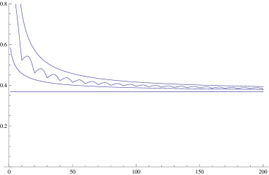
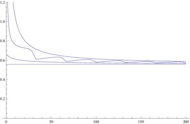
Figure 1: Graph of the error rate function $n\mapsto-\log(e_{n}(0))/n$, together with lower and upper bounds. Starting from below we have the Chernoff bound (the constant), the lower bound (49), the exact error rate (the oscillating line), and the upper bound (48); the two cases considered are (a) for $p=0.001$ and $q=0.5$, and (b) for $p=10^{-10}$ and $q=0.5$.

References

- [1] K.M.R. Audenaert: A sharp Fannes-type inequality for the von Neumann entropy; J. Phys. A 40, 8127–8136, (2007)
- [2] K.M.R. Audenaert, J. Calsamiglia, Ll. Masanes, R. Munoz-Tapia, A. Acin, E. Bagan, F. Verstraete.: Discriminating states: the quantum Chernoff bound; Phys. Rev. Lett. 98 160501, (2007)
- [3] K.M.R. Audenaert, M. Nussbaum, A. Szkoła, F. Verstraete: Asymptotic error rates in quantum hypothesis testing; Commun. Math. Phys. 279, 251–283 (2008).
- [4] R.R. Bahadur, R.R. Rao: On deviations of the sample mean; The Annals of Mathematical Statistics, vol. 31, no. 4, 1015–1027, (1960)
- [5] A. Barvinok: A course in convexity; American Mathematical Society, Providence, (2002)
- [6] R. Bhatia: Matrix Analysis; Springer, (1997)
- [7] I. Bjelakovic, R. Siegmund-Schultze: An ergodic theorem for the quantum relative entropy; Comm. Math. Phys. 247, 697–712, (2004)
- [8] F.G.S.L. Brandao, M.B. Plenio: A Generalization of Quantum Stein’s lemma; Comm. Math. Phys. 295, 791–828, (2010)
- [9] J.A. Bucklew, J.S. Sadowsky: A contribution to the theory of Chernoff bounds; IEEE Trans. Inform. Theory 39, no. 1, pp. 249–254, (1993)
- [10] I. Csiszár, J. Körner: Information Theory; 2nd edition, Cambridge University Press, (2011)
- [11] A. Dembo, O. Zeitouni: Large Deviations Techniques and Applications ; Second ed., Springer, Application of Mathematics, Vol. 38, (1998)
- [12] I. Ekeland, R. Temam: Convex Analysis and Variational Problems; North-Holland, American Elsevier (1976)
- [13] M. Fannes: A continuity property of the entropy density for spin lattice systems; Commun. Math. Phys., 31, 291–294, (1973)
- [14] W. Feller: An Introduction to Probability and Its Applications, Vol. I., John Wiley & Sons, Inc., (1966)
- [15] M. Hayashi, T. Ogawa: On error exponents in quantum hypothesis testing; IEEE Trans. Inf. Theory, vol. 50, issue 6, pp. 1368–1372, (2004)
- [16] M. Hayashi: Error exponent in asymmetric quantum hypothesis testing and its application to classical-quantum channel coding; Phys. Rev. A 76, 062301, (2007).
- [17] C.W. Helström: Quantum Detection and Estimation Theory; Academic Press, New York, (1976)
- [18] F. Hiai, D. Petz: The proper formula for relative entropy and its asymptotics in quantum probability; Comm. Math. Phys. 143, 99–114 (1991).
- [19] F. Hiai, D. Petz: Entropy densities for algebraic states; J. Funct. Anal. 125, 287–308 (1994)
- [20] F. Hiai, M. Mosonyi, T. Ogawa: Large deviations and Chernoff bound for certain correlated states on a spin chain; J. Math. Phys. 48, (2007)
- [21] F. Hiai, M. Mosonyi, T. Ogawa: Error exponents in hypothesis testing for correlated states on a spin chain; J. Math. Phys. 49, 032112, (2008)
- [22] F. Hiai, M. Mosonyi, M. Hayashi: Quantum hypothesis testing with group symmetry; J. Math. Phys. 50 103304 (2009)
- [23] W. Hoeffding: Asymptotically optimal tests for multinomial distributions; The Annals of Mathematical Statistics, vol. 36, no. 2, pp. 369–401, (1965)
- [24] A.S. Holevo: On Asymptotically Optimal Hypothesis Testing in Quantum Statistics; Theor. Prob. Appl. 23, 411-415, (1978)
- [25] V. Jaksic, Y. Ogata, C.-A. Pillet, R. Seiringer: Quantum hypothesis testing and non-equilibrium statistical mechanics; Rev. Math. Phys. 24, no. 6, 1230002, (2012)
- [26] Ke Li: Second order asymptotics for quantum hypothesis testing; arXiv:1208.1400, (2012)
- [27] M. Mosonyi, F. Hiai, T. Ogawa, M. Fannes: Asymptotic distinguishability measures for shift-invariant quasi-free states of fermionic lattice systems; J. Math. Phys. 49, 072104, (2008)
- [28] M. Mosonyi: Hypothesis testing for Gaussian states on bosonic lattices; J. Math. Phys. 50, 032104, (2009)
- [29] H. Nagaoka: Strong converse theorems in quantum information theory; in the book “Asymptotic Theory of Quantum Statistical Inference” edited by M. Hayashi, World Scientific, (2005)
- [30] H. Nagaoka: The converse part of the theorem for quantum Hoeffding bound; quant-ph/0611289
- [31] H. Nagaoka, M. Hayashi: An information-spectrum approach to classical and quantum hypothesis testing for simple hypotheses; IEEE Trans. Inform. Theory 53, 534–549, (2007)
- [32] M. Nussbaum, A. Szkoła: A lower bound of Chernoff type for symmetric quantum hypothesis testing; Ann. Statist. 37, 1040–1057, (2009)
- [33] T. Ogawa, H. Nagaoka: Strong converse and Stein’s lemma in quantum hypothesis testing; IEEE Trans. Inform. Theory 47, 2428–2433 (2000).
- [34] D. Petz: Quasi-entropies for finite quantum systems; Rep. Math. Phys. 23, 57–65, (1986)
- [35] D. Petz: Quantum Information Theory and Quantum Statistics; Theoretical and Mathematical Physics, Springer, (2008)
- [36] N.P. Salikhov: On strengthening Chernoff’s inequality; Theory Probab. Appl. 37, no. 3, pp. 564–567, (1992)
- [37] M. Tomamichel, R. Colbeck, R. Renner: A fully quantum asymptotic equipartition property; IEEE Trans. Inform. Theory 55, 5840–5847, (2009)
- [38] M. Tomamichel: A framework for non-asymptotic quantum information theory; PhD thesis, ETH Zürich, (2006)