Chaos in elliptical galaxies

Abstract

Here I present a review of the work done on the presence and effects of chaos in elliptical galaxies plus some recent results we obtained on this subject. The fact that important fractions of the orbits that arise in potentials adequate to represent elliptical galaxies are chaotic is nowadays undeniable. Alternatively, it has been difficult to build selfconsistent models of elliptical galaxies that include significant fractions of chaotic orbits and, at the same time, are stable. That is specially true for cuspy models of elliptical galaxies which seem to best represent real galaxies. I argue here that there is no physical impediment to build such models and that the difficulty lies in the method of Schwarzschild, widely used to obtain such models. Actually, I show that there is no problem in obtaining selfconsistent models of elliptical galaxies, even cuspy ones, that contain very high fractions of chaotic orbits and are, nevertheless, highly stable over time intervals of the order of a Hubble time.

LECTURE

(1) Facultad de Ciencias Astronómicas y Geofísicas - UNLP
(2) Instituto de Astrofísica de La Plata (CCT CONICET La Plata - UNLP)

1. Models of elliptical galaxies

How can we build a dynamical model of an elliptical galaxy? The basic constituents of galaxies are dark matter, stars and gas (plus a little dust). Gas dynamics plays a significant role in the formation process of all galaxies, but their influence in full-fledged elliptical galaxies is negligible, so that only dark matter and stars need to be taken into account for models that represent them. Thus, Newtonian dynamics is all that is needed to model elliptical galaxies and even a black hole can be represented simply as a point mass for our purposes.

The effects of star-star interactions can be neglected for these models, as is shown in any textbook on galactic dynamics (see, e.g., Binney & Tremaine 2008), and we can assume that there is a smooth distribution of mass density (dark matter plus stars) that creates a similarly smooth potential. Let us consider now the types of orbits we found in elliptical galaxies.

1.1. Typical orbits in elliptical galaxies

A significant breakthrough in elliptical galaxies dynamics was done with the use of Stäckel potentials that are fully integrable, so that all orbits are regular. In particular, de Zeeuw & Lynden-Bell (1985), de Zeeuw (1985) and Statler (1987) investigated the "perfect ellipsoid", whose density is given by:

$$\rho(r)=\frac{\rho_{o}}{(1+m^{2})^{2}}\,$$ (1)

where $m$ is the ellipsoidal radius:

$${m^{2}}=\frac{x^{2}}{a^{2}}+\frac{y^{2}}{b^{2}}+\frac{z^{2}}{c^{2}}.\,$$ (2)

Although that model is no longer regarded as an adequate representation of elliptical galaxies, its main kinds of orbits are also found in the more realistic models we use nowadays. They are: a) Boxes, that can come as close as one wishes to the center of the model and do not keep the sense of rotation; b) Minor axis tubes, that never come close to the center and rotate always in the same sense around the minor axis of the model; c) Major axis tubes, that never come close to the center either and always rotate in the same sense around the major axis of the model, they are in turn divided in inner and outer major axis tubes.

There is no reason, other than mathematical simplicity, to adopt the perfect ellipsoid, or any other Stäckel potential for that matter, to model elliptical galaxies. On the contrary, it has a flat central density distribution and we know nowadays that cuspy galaxies are the rule (we will return to this point later on). In cuspy models the box orbits tend to be replaced by "boxlets", i.e., resonant orbits that avoid the center of the model (Miralda-Escudé & Schwarzschild 1989).

All these are regular orbits and, of course, in generic potentials we have also chaotic orbits but, since chaos is the main subject of the present lectures, they will be analyzed in much more detail later on.

1.2. The problem of self-consistency

The galactic models must be self-consistent, that is, the mass distribution creates a gravitational field where certain kinds of orbits are possible, and those orbits should be such that they yield that mass distribution. The Poisson and Boltzmann equations can be used to obtain simple spherical or disk models (see, e.g., Binney and Tremaine 2008), but special methods are required for the triaxial models needed for elliptical galaxies.

One of the most popular of those methods is the one due to Schwarzschild (1979). First, one chooses a reasonable mass distribution and obtains its potential. A library of orbits is then computed in that potential using a variety of initial conditions in order to cover all the possible orbits in that potential, and weights are assigned according to the time that a particle on each orbit would spent in every region of the available space. Those weights are subsequently used to set a system of linear equations that related the density in every region to the fraction of orbits that make up the system. Finally, solving that system, the fraction of every kind of orbit is obtained.

This method certainly offers a straightforward way of obtaining a self-consistent model, but there are several details that should be taken into account. To begin with, there is not a single solution, and one does not know a priori towards which solution the method will converge. Besides, the chosen initial mass distribution conditions the results, for example, choosing the mass distribution of the perfect ellipsoid given above will force the system to have constant axial ratios, $b/a$ and $c/a$, from the center through the outermost regions of the model. It is not easy to guarantee that all the possible kinds of orbits have been included in the library and, to make this problem worse, the libraries are usually not very large, from several hundreds of orbits at Schwarschild’s time and up to a few tens of thousands nowadays (see, e.g., Capuzzo-Dolcetta et al. 2007).

The most serious problem to the method of Schwarzschild is the one posed by chaotic orbits, which can display very different behavior at different time intervals, even over long periods of time. Sticky orbits, in particular, can mimic regular orbits over long intervals, only to reveal their true chaotic nature later on. Schwarzschild (1993) realized that chaotic orbits were all too frequent in triaxial models and he tried to include them in his models but, then, the models did not remain stationary. He computed models with orbits integrated over one Hubble time and, then, new models using the same orbits but integrated between two and three Hubble times. Differences beween equivalent models were revealed, e.g., by differing axial ratios, as shown by Table 1.

Table 1.: Axial ratio changes in the models of Schwarzschild (1993).

$c/a$	$b/a$	$\Delta(c/a)$	$\Delta(b/a)$
0.7	0.8631	-4.3%	-7.3%
0.5	0.7906	2.6%	-3.9%
0.3	0.7382	10.0%	0.9%
0.3	0.9534	4.3%	0.6%
0.3	0.4254	16.7%	16.4%
0.3	0.3289	6.7%	3.4%

Of course, it would be obviously hopeless to try to use observations to detect such small changes, so that we might ask: If we cannot recognize a truly stable galaxy from a slowly evolving one, why care? Nevertheless, from a theoretical point of view, it is certainly important. Therefore, the question we should be actually asking is: Is it possible to have a stable self-consistent system if a significant fraction of its material is in chaotic motion? No doubt, most dynamicists will feel inclined to answer "No" to that question (see, e.g., Siopis and Kandrup 2000) but, as I will show, they will be wrong.

From the observational point of view there is proof, both statitical (e.g., Ryden 1996) and on individual galaxies (e.g., Statler et al.), that at least some elliptical galaxies are triaxial, and not merely rotationally symmetric (either oblate or prolate). Moreover, the surface brightness of elliptical galaxies increases towards the center forming a "cusp" (e.g., Crane et al. 1993, Moller et al. 1995) that reveals the presence of central mass concentration and, probably, a black hole. The problem is that it has long been known (see, e.g., Gerhard & Binney 1985) that central cusps and black holes can disrupt the box orbits that are necessary to keep the triaxial form. The strong central field reorients the box and chaotic orbits that come close to the center, so that a triaxial model will quickly evolve into a rotationally symmetric one (we will return to this point later on). Is it then possible to have cuspy triaxial galaxies? Can such galaxies have significant amounts of matter on chaotic orbits? These questions are obviously important from an observational point of view and for fitting models to the observations.

1.3. The problem of diffusion

Several authors haven been worried by the "problem" of chaotic mixing and, for that reason, they have tried to avoid including chaotic orbits in their models. For example, Merritt and Fridman (1996) refer to solutions that contain chaotic orbits as quasi equilibrium and indicate that in quasi equilibrium models chaotic mixing will produce a slow evolution of the model figure, specially near the center. That idea comes from the assumption that, in the long run, chaotic orbits will cover uniformly all the space available to them by the energy integral, i.e., a region much rounder than the triaxial model, but that assumption is simply wrong. Chaotic orbits do not occupy all the space available to them and live there forever happily. First, they do not occupy all the space allowed to them by the energy integral because there are usually "islands of stability" where chaotic orbits cannot enter and, second, they may at times behave similarly to regular orbits. The more or less chaotic behavior of a chaotic orbit can be easily followed, for example, computing the finite time Lyapunov numbers (FTLNs hereafter) that increase, or decrease, as the orbit behaves more, or less, chaotically. As shown by Muzzio et al. (2005), if one sorts the fully chaotic orbits according to the values of those numbers, one finds that the orbits with lower values give a more triaxial distribution than the orbits with higher values.

The actual problem posed by the changing behavior of chaotic orbits is the one they pose to the method of Schwarzschild. The method will favor the inclusion of orbits elongated in the direction of the major axis but, when those orbits begin to behave more chaotically, the shape of the model will become rounder. This effect could be compensated if the model includes chaotic orbits that initially had a rounder distribution and, later on, a more elongated one. In other words, one might have a dynamic equilibrium: a given chaotic orbit will not occupy always the same region of space (as regular orbits do) but, as it moves out to occupy a different zone, another chaotic orbit will fill in the region left vacant by the former. I will show later on that it is perfectly possible to achieve such dynamical equilibrium and to get stable models that include large fractions of chaotic orbits, but one has to resort to methods different from Schwarzschild’s. One cannot see any simple way to take into account the abovementioned effect in that method, and the situation is even worse when constant axial ratios are used throughout the model. As indicated by Muzzio et al. (2005), in that case one has no rounder halo that could act as a reservoir of chaotic orbits that, as time goes by, become more elongated and compensate for those that, on the contrary, become rounder. In fact, stable triaxial models that include high fractions of chaotic orbits become rounder as one goes farther from the center of the system (see, e.g., Muzzio et al. 2005, Aquilano et al. 2007).

1.4. Central black holes

The effects of a central growing black hole on the dynamics of a triaxial system were well described by Merritt and Quinlan (1998), who built an $N$-body model of a triaxial galaxy and verified that it was stable. They then let a black hole grow at the center of the model and, as could be expected, the central density distribution became much steeper. But it also turned out that the model lost its triaxiality and the evolution was faster for more massive black holes. The central regions became rounder, but even the outermost regions were affected.

Rather different results were obtained by Poon & Merrit (2002, 2004) who obtained equilibrium models of the central regions of triaxial galaxies containing black holes and checked their stability. They were able to find stable configurations that persisted even within the sphere of influence of the black hole. Interestingly, their models included chaotic orbits as well as regular ones. These results seem to be at odds with other work, like that of Merritt & Quinlan (1998). It is possible that the fact that the models were built including the black hole, rather than letting it grow after the model was built, might help to explain the difference.

2. Chaotic orbits in elliptical galaxies

The presence of chaotic orbits in triaxial potentials was noticed early on, even in the original paper of Schwarzschild (1979). Moreover, in Schwarzschild (1993), which dealt with the singular (i.e., cuspy) logarithmic potential, he showed that many orbits that resulted from his "initial condition spaces" were indeed chaotic.

More recently, after the acceptance that elliptical galaxies are cuspy and that most of them may be harboring central black holes, it was found that both cuspiness and central black holes enhance the chaotic effects. These studies of orbits are usually performed on fixed and smooth potentials, such as the one arising from the triaxial generalization of the model of Dehnen (1993), whose density distribution is:

$$\rho(m)=\frac{(3-\gamma)aM}{4\pi}m^{-\gamma}(m+d)^{-(4-\gamma)}\;\;\;\;{\rm with}\;\;\;\;0\leq\gamma<3,$$ (3)

where $m$ is the triaxial radius already defined by equation (2), $M$ is the total mass, $d$ is a scale parameter proportional to the effective radius (i.e., the radius containing half of the mass) and $\gamma$ parametrizes the slope of the central cusp. Merritt and Fridman (1996) provided the corresponding equations for the potential, the forces and the derivatives of the forces (which are needed for the variational equations that allow the computation of the Lyapunov exponents). Those expresions involve rather complicated integrals and must be solved numerically.

The axial ratios $b/a$ and $c/a$ give an idea of the flatness of the model, and it is usual to measure the triaxiality, $T$, as:

$$T=\frac{(a^{2}-b^{2})}{(a^{2}-c^{2})}.$$ (4)

It goes from 0, for an oblate spheroid, to 1, for a prolate spheroid, and the ellipsoids with $T=0.5$ are called "maximally triaxial" ellipsoids.

Merritt and Fridman (1996) investigated maximally triaxial models with $\gamma=1$ (weak-cusp) and $\gamma=2$ (strong-cusp). Their libraries of orbits contained high fractions of chaotic orbits, particularly in the strong-cusp case and for orbits with zero initial velocity. Thus, it is not surprising that the attempts to build stable models without chaotic orbits were doomed to failure. Using the method of Schwarzschild, Merritt and Fridman managed to build "fully mixed" models for their weak-cusp case, but not for the strong-cusp one.

2.1. The contribution of Kandrup and Siopis

Siopis and Kandrup (2000) and Kandrup and Siopis (2003) did two very comprehensive investigations of orbits in the triaxial Dehnen potential, allowing also for the presence of a central black hole. They considered different axial ratios, cusp slopes and black hole masses and, in addition to the chaoticity of the orbits, they also investigated chaotic diffusion and how it is affected by noise.

They found that chaotic orbits tend to be extremely sticky for all cusp slopes, but specially for the steepest ones. This fact was revealed by visual inspection of the orbits, but also by the bimodal distribution of the FTLNs. Besides, if the orbits were not sticky, the FTLNs should fall as $t^{-1/2}$, where $t$ is the integration time, but they found a much lower slope, corroborating the stickiness. Moreover, the presence of a black hole increased the stickiness of the orbits. Except for the steepest cusp, the $\it fractions$ of chaotic orbits were not much affected by either the steepness of the cusp or the mass of the black hole. Nevertheless, the $\it values$ of the FTLNs were significantly affected by both: steeper cusps and more massive black holes led to larger FTLN values. They investigated the effect of triaxiality adopting $a=1.0$, $c=0.5$ and selecting different $b$ values. As could be expected, the fractions of chaotic orbits decreased both toward $b=0.5$ (prolate spheroid) and toward $b=1.0$ (oblate spheroid). Besides, going toward the innermost regions of the model the fraction of chaotic orbits increased, and also increased the effect of the mass of the black hole on that fraction. They also found that prolate spheroids tend to have larger fractions of chaotic orbits, and with larger FTLNs, than oblate spheroids; that effect was more pronounced for the outermost shells. Finally they considered changing both $b$ and $c$ adopting $b=1-D$ and $c=1-2D$, i.e., from a spherical system for $D=0$, to a disk for $D=0.5$. The fraction of chaotic orbits turned out to increase monotonically with $D$, and even a very small departure from sphericity yielded chaos. Without a black hole, the size of the FTLNs also increased monotonically with $D$. Larger black hole masses resulted in larger FTLN values, but the increase with $D$ leveled off for the most massive ones.

Chaotic mixing is another interesting aspect of the work of Kandrup and Siopis. They showed that different ensembles of chaotic orbits diffuse in different ways and end up occupying different regions even after long times. A very interesting aspect of their work is that they recognized that galaxies are subject to several perturbations that can be modelled as "noise" and profoundly affect chaotic diffusion. They considered: a) Periodic driving, to simulate the effect of a satellite orbiting the galaxy; b) Friction and white noise to simulate discreteness effects; c) Coloured noise to simulate the effects of encounters with other galaxies. They showed that all these effects tend to increase the diffusion rate.

2.2. Partially and fully chaotic orbits

Since we are interested in equilibrium models of elliptical galaxies, the energy integral always holds. Regular orbits have two additional isolating integrals, but we can have chaotic orbits either without any other isolating integral (fully chaotic orbits), or with just one (partially chaotic orbits). This difference had been recognized long ago (Contopoulos et al. 1978, Pettini & Vulpiani 1984), but little importance was assigned to it in galactic dynamics studies despite being found in several investigations of triaxial systems (e.g., Goodman and Schwarzschild 1981, Merritt and Valluri 1996). These studies used a sort of three dimensional (3-D) Poincaré map. If the velocity on an orbit is computed every time that the particle returns to the same point, then: a) The velocities of fully chaotic orbits will adopt any possible direction; b) Those of partially chaotic orbits will fall on a curve; c) The velocities of regular orbits will have always the same, or at most a finite number, of directions. Needless to say, this sort of 3-D Poincaré map is extremely computer time consuming, because one has to follow the orbit over very long time intervals to have a significant number of returns (almost) to the same point. A more efficient, albeit also computer time consuming, method is to compute all (and not just the largest) Lyapunov exponents: the exponents of regular orbits are all zero, partially chaotic orbits have one positive exponent, and fully chaotic orbits have two positive exponents. Using Lyapunov exponents Muzzio (2003) showed that, in triaxial models of elliptical galaxies, the spatial distributions of partially and fully chaotic orbits are diferent, so that it is important to separate them in studies of galactic dynamics. Similar results were obtained by Muzzio and Mosquera (2004) with models of galactic satellites and by Muzzio et al. (2005), Aquilano et al. (2007), Muzzio et al. (2009) and Zorzi (2011) with models of elliptical galaxies.

The Lyapunov exponents should be obtained integrating the orbit over an infinite time interval but, as that is impossible for numerically integrated orbits, the FTLNs are used instead. That rises the problem that one cannot reach zero values, even for regular orbits: if $T$ is the integration interval, then the lowest FTLN values will be of the order of $\ln T/T$. Besides, one might ask which is the practical limiting value to separate regular from chaotic orbits. The inverse of the Lyapunov exponent is called the Lyapunov time, and it gives the time scale for the exponential divergence of the orbit. At first sight, orbits with Lyapunov times longer than the Hubble time could be regarded as regular, but one should recall that what actually interests in galactic dynamics is the orbital distribution, rather than the exponential divergence of orbits. Therefore, the right question to ask is which is the limiting value of the Lyapunov exponents that separates orbits whose distribution is similar to that of regular orbits from those that have a clearly different distribution. Aquilano et al. (2007), Muzzio et al. (2009) and Zorzi (2011) investigated this problem and found that, for their models, the limiting value corresponds to a Lyapunov time about six or seven times larger than the Hubble time. In other words, orbits not chaotic enough to experience significant exponential divergence on a Hubble time are, nevertheless, chaotic enough to have a distribution significantly different from that of regular orbits. It should be noted, however, that the computed fraction of chaotic orbits is not substantially altered by the limiting value selected: for the models of the authors cited, adopting the limit corresponding to six or seven Hubble times may result in a fraction of chaotic orbits of, say, $40\%$ as compared to $35\%$ for the limit corresponding to one Hubble time.

3. The $N$-body method

The method of Schwarzschild (1979) is not the only one available to obtain equilibrium models of elliptical galaxies. Actually, self-consistent models of triaxial systems had been obtained earlier using the $N$-body method (see, e.g., Aarseth & Binney 1978). One starts with a certain distribution of mass points and follows its evolution using an $N$-body code to integrate the equations of motion. A wise selection of the initial distribution, or a little tinkering with the code, allows one to obtain a stable triaxial system whose self-consistency is assured by the use of the $N$-body code.

One can begin, for example, with a spherical distribution of mass points with very small velocities. Gravity will force the collapse of such system and the radial orbit instability will lead it toward a triaxial equilibrium distribution (see, e.g., Aguilar & Merritt 1990). One can change the initial velocity dispersion to obtain systems with different triaxiality: the smaller the dispersion, the larger the triaxiality. This method has been used by Voglis et al. (2002), Kalapotharakos and Voglis (2005), and by my coworkers and myself. Another possibility is to launch one stellar system against another and let them merge, yielding a triaxial system, a strategy followed, e.g., by Jesseit et al. (2005).

Code tinkering was used, for example, by Holley-Bockelmann et al. (2001) who started with a Dehnen (1993) spherical distribution of mass points and added to the $N$-body code a fictious force that slowly squeezed the system, first in the $z$ direction, and then in the $y$ direction. The original $N$-body code was finally used to let the system relax toward a final triaxial equilibrium distribution.

After building the triaxial system, one has to investigate its orbital structure. The $N$-body code is no longer useful because its potential is neither smooth (because it is the sum of the potentials of the individual particles) nor time independent (due to the statistical changes in the distribution of the finite number of particles). Therefore, a smooth and time independent approximation should be adopted for the potential and then, orbits in that potential can be computed using as initial conditions the positions and velocities of all, or a random sample of, the mass points. One can then separate regular from chaotic orbits, and partially from fully chaotic orbits, with an adequate chaos indicator and, finally, the different kinds of regular orbits can be obtained with an automatic classification code based, e.g., on the analysis of the orbital frequencies.

Both Schwarzschild’s and the $N$-body method end up with the same result: an equilibrium self-consistent triaxial system and the knowledge of its orbital content. The steps to reach those results are, however, different. One uses the orbits to obtain the system in Schwarzschild’s method, while in the $N$-body method the system is built by the gravitational interactions mimicked by the $N$-body code and thereafter one performs the orbital analysis.

3.1. The work of the Athens’ group

Voglis et al. (2002) obtained two non-cuspy stable triaxial models, Q (Quiet) and C (Clumpy), from cold collapses of initially spherical particle distributions. The fractions of chaotic orbits were $32\%$ for the former and $26\%$ for the latter. A similar model was built and investigated by Kalapotharakos and Voglis (2005), who found $32\%$ of chaotic orbits. An interesting point that they raised is that the real particles in their model did not cover all the space that one could cover with test particles. It is a natural consequence of self-consistency, that only allows the presence of certain orbits, and Kalapotharakos and Voglis showed this effect beautifully on the frequency map. A very clever aspect of their work is that they determined the orbital frequencies of the chaotic orbits, in addition to those of the regular orbits, and showed that, due to the stickiness, many of them fall close to the loci of the regular orbits on the frequency map. Again, their model is stable but, after the sudden introduction in it of a central black hole, it quickly evolves toward an oblate shape.

More recently, Kalapotharakos (2008) investigated the evolution of two stable, non-cuspy, triaxial systems after the introduction of a central black hole. He linked that evolution to the presence of chaotic orbits and introduced a parameter, dubbed effective chaotic momentum, that correlates well with the rate of evolution of the system.

3.2. The puzzles of the work of Holley-Bockelmann et al.

As already mentioned, Holley-Bockelmann et al. (2001) obtained cuspy triaxial systems through adiabatical deformation of Dehnen (1993) spherical models. Their systems turned out to be very stable, but they found very little chaos (less than $1\%$, and they even attributed that little to noise in their potential approximation), in complete contradiction with the results of the Athen’s group and our own. Kandrup & Siopis (2003) pointed out that the Fourier technique used by Holley-Bockelmann et al. could have made them miss many chaotic orbits, a likely possibility considering that such technique is not as good as others for chaos detection (see, e.g., Fig. 2 of Kalapotharakos and Voglis 2005). Nevertheless, one should recall that the collapses used by the Athens’ group and ourselves to build triaxial models yield predominantly radial orbits, which have long been known to favor chaos (see, e.g., Martinet 1974), while the adiabatical squeezing used by Holley-Bockelman et al. probably resulted in a more isotropic velocity distribution, so that the discrepancy among the chaotic fractions might be real.

In a second paper, Holley-Bockelmann et al. (2002) let a black hole grew at the center of one of their models. As could be expected, they found that the central cusp became steeper and the central regions rounder. But the outer regions (even those that contained the inner $10\%$ of the total mass) retained the triaxial shape. Just as mentioned before about the work of Poon and Merritt (2002, 2004), these results seem to be at odds with other investigations, like that of Merritt & Quinlan (1998).

3.3. The work of our La Plata-Rosario group

In our first works we used 100,000 particles to build our $N$-body models, and for the past few years we have been using one million, guaranteeing in any case the accuracy of stability studies. Besides, we typically classify between 3,000 and 5,000 orbits per model, which provides adequate statistics. To build our models we just use the simple cold collapse technique and we do not try to follow the actual galaxy formation process, because we are not interested in that process but only in obtaining models morphologically similar to elliptical galaxies. For example, although it is not physically realistic, we let our models relax during intervals of several Hubble times to ensure that our subsequent studies refer to equilibrium models.

Muzzio et al. (2005) obtained a model of a non-cuspy E6 galaxy that contained $52.7\%$ of chaotic orbits. Later on, Muzzio (2006) found that the model displayed very slow figure rotation (i.e., it rotated despite having zero angular momentum). Taking the rotation into account, the fraction of chaotic orbits raised to $56.6\%$, probably because of the symmetry breaking caused by the rotation, despite its small value. Later on, Aquilano et al. (2007) obtained three models of non-cuspy galaxies resembling elliptical galaxies of types E4 through E6, all of them very stable and with between one third and two thirds of chaotic orbits. All these models had axial ratios that increased from the center toward the outer parts of the galaxy, which may have contributed to them being stable and chaotic at the same time. Besides, all of them corroborated the need to distinguish partially from fully chaotic orbits because their spatial distributions were different.

Muzzio et al. (2009) managed to obtain cuspy models of E4 and E6 galaxies that, again, were highly stable despite having about two thirds of chaotic orbits. Nevertheless, those models had pushed to the limit the use of the $N$-body code of Aguilar (see, White 1983 and Aguilar and Merritt 1990) and, in fact, they had to introduce a small additional potential to compensate for the softening needed by the code. Therefore, in order to continue investigating cuspy models, we switched to the code of Hernquist (Hernquist and Ostriker 1992) that needs no softening and uses a radial expansion of the potential in functions related to the potential of Hernquist (1990) which is itself cuspy with $\gamma=1$. Our first work with this code is the PhD thesis of Zorzi (2011), defended last June at the Universidad Nacional de Rosario.

Kalapotharakos et al. (2008) investigated the approximation of $N$-body realizations of models of Dehnen (1993) for different values of $\gamma$ using the self-consistent field method (the method of Hernquist & Ostriker 1992 is just a special case of that method), and they found that the choice of the radial basis functions seriously affected the results obtained on chaotic orbits. Nevertheless, the method of Hernquist & Ostriker turned out to be adequate for models with $\gamma\simeq 1$, and we had selected the number of terms in the potential expansion so as to have models whose cusps had that slope (Zorzi & Muzzio 2009).

Zorzi (2011) built four groups of models that mimic E2, E3, E4 and E5 galaxies. Each group consisted of three models that differed only in the seed number used to randomly generate the initial conditions. In other words, for each galaxy type she had three statistically equivalent models, which is important to control the consistency and robusteness of the results to be obtained from them. In fact, except for the figure velocity rotation, all her results were essentially the same for statistically equivalent models. Figure 1 gives the logarithmic density vs. radius plot for the central regions of her E4 models and we can notice the excellent agreement among the different realizations of the model, as well as the $\gamma\simeq 1$ cusp.

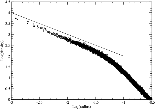
Figure 1.: The logarithm of the density vs. the logarithm of the radius for the E4 models of Zorzi (2011). Filled and open circles and crosses correspond to three statistically equivalent realizations of the same model. The slope of the straight line is equal to 1.

To check the stability of the models, she computed their central density and their three moments of inertia over intervals of the order of five Hubble times. The changes in those quantities were very small, indeed, smaller than $2.7\%$ in one Hubble time in all cases. Moreover, she showed that most of that change is most likely due to relaxation effects in the $N$-body code (see Hernquist & Barnes 1990). Not only are these values smaller than most of those of Schwarzschild shown in Table 1, but Zorzi’s had been obtained with self-consistent models, while Schwarzschild’s correspond to a fixed potential. Actually, when the potential is fixed, the changes in the models of Zorzi are an order of magnitude smaller than those obtained self-consistently. The fractions of chaotic orbits are extremely high in Zorzi’s models, up to more than $85\%$ for her E2 and E5 models, and larger that $75\%$ for the other two. The values of the FTLNs are also very high, almost twice the values of the equivalent non-cuspy models of Aquilano et al. (2007). And, as in our previous work, she also found that partially and fully chaotic orbits have different distributions and should be analyzed separately.

4. Conclusions

The works of the Athens’ group and our own show that it is perfectly possible to build triaxial stellar systems, even cuspy ones, that include large fractions of chaotic orbits and are, nevertheless, highly stable over intervals of the order of one Hubble time. All these models were obtained using the $N$-body method, so that the difficulty to obtain such models with the method of Schwarzschild should be attributed to the method itself and not to physical causes.

We certainly need more models built with the adiabatic squeezing technique of Holley-Bockelmann et al. (2001). The orbits in those models are probably less radial than those in the models arising from cold collapses and that might result in lower fractions of chaotic orbits and models more capable of preserving triaxiality when harboring a black hole.

The distributions of partially and fully chaotic orbits are certainly different, but much remains to be done on this subject. Are the partially chaotic orbits merely confined to the stochastic layers around resonances? Or do they fill in connected regions where an isolating integral, or pseudo integral, holds? And, certainly, we need better and faster methods than that of the Lyapunov exponents to separate partially from fully chaotic orbits.

Modern observations suggest not only that elliptical galaxies have significant rotation, but that they even rotate in different directions at different distances from the center, perhaps a consequence of past mergers. Nevertheless, there are not many works on rotating ellipticals (a recent exception is that of Deibel et al. 2011) and more work is clearly warranted on this subject.

The figure rotation we found in many of our models is certainly puzzling. All the tests we made support that it is real and, besides, these models can be seen as the stellar counterpart of the Riemann ellipsoids of fluid dynamics. But why, appart from the tendency of flatter systems to rotate faster, the rotation shows no obvious connection to the properties of the model and, worst, why do statistically equivalent models display different rotation velocities? This is another subject where more research is clearly warranted.

Last but no least, let me end recalling that, although I have only briefly mentioned regular orbits here, their study is also very interesting. Not only are they important for the dynamics of elliptical galaxies, but they also offer technical challenges, like the design of fast and accurate methods of automatic classification.

Acknowledgements.

I am very grateful to C. Efthymiopoulos for useful comments and to R.E. Martínez and H.R Viturro for their technical assistance. This work was supported with grants from the Consejo Nacional de Investigaciones Científicas y Técnicas de la República Argentina, the Agencia Nacional de Promoción Científica y Tecnológica and the Universidad Nacional de La Plata.

References

Aarseth, S.J. & Binney, J., 1978, MNRAS, 185, 227

Aguilar, L.A., & Merritt, D., 1990, ApJ, 354, 33

Aquilano, R.O., Muzzio,J.C., Navone, H.D., & Zorzi, A.F., 2007, Celest. Mech. & Dynam. Astron., 99, 307

Binney, J., & Tremaine, S.J., 2008, Galactic Dynamics, Princeton University Press

Capuzzo-Dolcetta, R., Leccese, L., Merritt, D., Vicari, A., 2007, ApJ, 666, 165

Contopoulos, G., Galgani, L., & Giorgilli, A., 1978, Phys. Rev. A, 18, 1183

Dehnen W., 1993, MNRAS, 265, 250

Deibel, A.T., Valluri, M. & Merritt, D., 2011, ApJ, 728, 128

de Zeeuw, P.T., 1985, MNRAS, 216, 273

de Zeeuw, P.T., & Lynden-Bell, D., 1985, MNRAS, 215, 713

Gerhard, O.E., & Binney, J., 1985, MNRAS, 216, 467

Goodman, J., & Schwarzschild, M., 1981, ApJ, 245, 1087

Hernquist, L., 1990, ApJ, 356, 359

Hernquist, L., & Barnes, J., 1990, ApJ, 349, 562

Hernquist, L., & Ostriker, J.P., 1992, ApJ, 386, 375

Holley-Bockelmann, K., Mihos, J.C., Sigurdsson, S., & Hernquist, L., 2001, ApJ, 549, 862

Holley-Bockelmann, K., Mihos, J.C., Sigurdsson, S., Hernquist, L., & Norman, C., 2002, ApJ, 567, 817

Jaffe, W., Ford, H.C., O’Connell, R.W., van den Bosch, F.C., & Ferrarese, L., 1994, AJ, 108, 1567

Jesseit, R., Naab, T., & Burkert, A., 2005, MNRAS, 360, 1185

Kalapotharakos, C., 2008, MNRAS, 389, 1709

Kalapotharakos, C., Efthymiopoulos, C., & Voglis, N., 2008, MNRAS, 383, 971

Kalapotharakos, C., & Voglis, N., 2005, Celest. Mech. & Dynam. Astron., 92, 157

Kandrup, H.E., Siopis, C., 2003, MNRAS, 345, 727

Merritt, D., & Quinlan, G.D., 1998, ApJ, 498, 625

Merritt, D., & Valluri, M.,, 1996, ApJ, 471, 82

Miralda-Escudé, J., & Schwarzschild, M., 1989, ApJ, 339, 752

Moller, P., Stiavelli, M., & Zeilinger, W.W., 1995, MNRAS, 276, 979

Martinet, L., 1974, A&A, 32, 329

Muzzio, J.C., 2003, BAAA, 45, 69

Muzzio, J.C., 2006, Celest. Mech. & Dynam. Astron., 96, 85

Muzzio, J.C., Carpintero, D.D., Wachlin, F.C., 2005, Celest. Mech. & Dynam. Astron., 91, 173

Muzzio, J.C., Mosquera, M.E., 2004, Celest. Mech. & Dynam. Astron., 88, 379

Muzzio, J.C., Navone, H.D., & Zorzi, A.F., 2009, Celest. Mech. & Dynam.Astron., 105, 379

Pettini, M., & Vulpiani, A., 1984, Phys. Lett., 106A, 207

Poon, M.Y. & Merritt, D., 2002, ApJ, 568, 89

Poon, M.Y. & Merritt, D., 2004, ApJ, 606, 774

Ryden, B.S., 1996, ApJ, 461, 146

Schwarzschild, M., 1979, ApJ, 232, 236

Schwarzschild, M., 1993, ApJ, 409, 563

Siopis, C., Kandrup, H.E., 2000, MNRAS, 319, 43

Statler, T.S., 1987, ApJ, 321, 113, 1987

Statler, T.S., Emsellem, E., Peletier, R.F., & Bacon, R., 2004, MNRAS, 353, 1

Voglis N., Kalapotharakos C., & Stavropoulos I., 2002, MNRAS, 337, 619

White, S.D.M., 1983, ApJ, 274, 53

Zorzi, A.F., 2011, PhD Thesis, Universidad Nacional de Rosario, Argentina

Zorzi, A. F., & Muzzio, J. C., 2009, Memorias del II Congreso de Matemática Aplicada, Computacional e Industrial, Rosario