Atomic norm denoising with applications to line spectral estimation

Abstract

Motivated by recent work on atomic norms in inverse problems, we propose a new approach to line spectral estimation that provides theoretical guarantees for the mean-squared-error (MSE) performance in the presence of noise and without knowledge of the model order. We propose an abstract theory of denoising with atomic norms and specialize this theory to provide a convex optimization problem for estimating the frequencies and phases of a mixture of complex exponentials. We show that the associated convex optimization problem can be solved in polynomial time via semidefinite programming (SDP). We also show that the SDP can be approximated by an $\ell_{1}$-regularized least-squares problem that achieves nearly the same error rate as the SDP but can scale to much larger problems. We compare both SDP and $\ell_{1}$-based approaches with classical line spectral analysis methods and demonstrate that the SDP outperforms the $\ell_{1}$ optimization which outperforms MUSIC, Cadzow’s, and Matrix Pencil approaches in terms of MSE over a wide range of signal-to-noise ratios.

1 Introduction

Extracting the frequencies and relative phases of a superposition of complex exponentials from a small number of noisy time samples is a foundational problem in statistical signal processing. These line spectral estimation problems arise in a variety of applications, including the direction of arrival estimation in radar target identification [1], sensor array signal processing [2] and imaging systems [3] and also underlies techniques in ultra wideband channel estimation [4], spectroscopy [5], molecular dynamics [6], and power electronics [7].

While polynomial interpolation using Prony’s technique can estimate the frequency content of a signal exactly from as few as $2k$ samples if there are $k$ frequencies, Prony’s method is inherently unstable due to sensitivity of polynomial root finding. Several methods have been proposed to provide more robust polynomial interpolation [8, 9, 10] (for an extensive bibliography on the subject, see  [11]), and these techniques achieve excellent noise performance in moderate noise. However, the denoising performance is often sensitive to the model order estimated, and theoretical guarantees for these methods are all asymptotic with no finite sample error bounds. Motivated by recent work on atomic norms [12], we propose a convex relaxation approach to denoise a mixture of complex exponentials, with theoretical guarantees of noise robustness and a better empirical performance than previous subspace based approaches.

Our first contribution is an abstract theory of denoising with atomic norms. Atomic norms provide a natural convex penalty function for discouraging specialized notions of complexity. These norms generalize the $\ell_{1}$ norm for sparse vector estimation [13] and the nuclear norm for low-rank matrix reconstruction [14, 15]. We show a unified approach to denoising with the atomic norm that provides a standard approach to computing low mean-squared-error estimates. We show how certain Gaussian statistics and geometrical quantities of particular atomic norms are sufficient to bound estimation rates with these penalty functions. Our approach is essentially a generalization of the Lasso [16, 17] to infinite dictionaries.

Specializing these denoising results to the line spectral estimation, we provide mean-squared-error estimates for denoising line spectra with the atomic norm. The denoising algorithm amounts to soft thresholding the noise corrupted measurements in the atomic norm and we thus refer to the problem as Atomic norm Soft Thresholding (AST). We show, via an appeal to the theory of positive polynomials, that AST can be solved using semidefinite programming (SDP) [18], and we provide a reasonably fast method for solving this SDP via the Alternating Direction Method of Multipliers (ADMM) [19, 20]. Our ADMM implementation can solve instances with a thousand observations in a few minutes.

While the SDP based AST algorithm can be thought of as solving an infinite dimensional Lasso problem, the computational complexity can be prohibitive for very large instances. To compensate, we show that solving the Lasso problem on an oversampled grid of frequencies approximates the solution of the atomic norm minimization problem to a resolution sufficiently high to guarantee excellent mean-squared error (MSE). The gridded problem reduces to the Lasso, and by leveraging the Fast Fourier Transform (FFT), can be rapidly solved with freely available software such as SpaRSA [21]. A Lasso problem with thousands of observations can be solved in under a second using Matlab on a laptop. The prediction error and the localization accuracy for line spectral estimation both increase as the oversampling factor increases, even if the actual set of frequencies in the line spectral signal are off the Lasso grid.

We compare and contrast our algorithms, AST and Lasso, with classical line spectral algorithms including MUSIC [8],and Cadzow’s  [22] and Matrix Pencil [10] methods . Our experiments indicate that both AST and the Lasso approximation outperform classical methods in low SNR even when we provide the exact model order to the classical approaches. Moreover, AST has the same complexity as Cadzow’s method, alternating between a least-squares step and an eigenvalue thresholding step. The discretized Lasso-based algorithm has even lower computational complexity, consisting of iterations based upon the FFT and simple linear time soft-thresholding.

1.1 Outline and summary of results

We describe here our approach to a general sparse denoising problem and later specialize these results to line spectral estimation. The denoising problem is obtaining an estimate $\hat{x}$ of the signal $x^{\star}$ from $y=x^{\star}+w$, where $w$ is additive noise. We make the structural assumption that $x^{\star}$ is a sparse non-negative combination of points from an arbitrary, possibly infinite set $\mathcal{A}\subset\mathbb{C}^{n}$. This assumption is very expressive and generalizes many notions of sparsity [12]. The atomic norm $\lVert\cdot\rVert_{\mathcal{A}}$, introduced in [12], is a penalty function specially catered to the structure of $\mathcal{A}$ as we shall examine in depth in next section, and is defined as:

$$\lVert x\rVert_{\mathcal{A}}=\inf\left\{t>0~{}\middle|~{}x\in t\operatorname{conv}(\mathcal{A})\right\}.$$

where $\operatorname{conv}(\mathcal{A})$ is the convex hull of points in $\mathcal{A}.$ We analyze the denoising performance of an estimate that uses the atomic norm to encourage sparsity in $\mathcal{A}$.

Atomic norm denoising.

In Section 2, we characterize the performance of the estimate $\hat{x}$ that solves

$$\mathop{\textrm{minimize}}_{x}\frac{1}{2}\lVert x-y\rVert_{2}^{2}+\tau\lVert x\rVert_{\mathcal{A}}.$$ (1.1)

where $\tau$ is an appropriately chosen regularization parameter. We provide an upper bound on the MSE when the noise statistics are known. Before we state the theorem, we note that the dual norm $\lVert\cdot\rVert_{\mathcal{A}}^{*}$, corresponding to the atomic norm, is given by

$$\lVert z\rVert_{\mathcal{A}}^{*}=\sup_{a\in\mathcal{A}}{\langle z,a\rangle},$$

where $\langle x,z\rangle=\mathop{\mathrm{Re}}(z^{*}x)$ denotes the real inner product.

Theorem 1.

Suppose we observe the signal $y=x^{\star}+w$ where $x^{\star}\in\mathbb{C}^{n}$ is a sparse nonnegative combination of points in $\mathcal{A}$. The estimate $\hat{x}$ of $x^{\star}$ given by the solution of the atomic soft thresholding problem (1.1) with $\tau\geq\operatorname{\mathbb{E}}\lVert w\rVert_{\mathcal{A}}^{*}$ has the expected (per-element) MSE

$$\frac{1}{n}\operatorname{\mathbb{E}}\lVert\hat{x}-x^{\star}\rVert_{2}^{2}\leq\frac{\tau}{n}\lVert x^{\star}\rVert_{\mathcal{A}}$$

This theorem implies that when $\operatorname{\mathbb{E}}\lVert w\rVert_{\mathcal{A}}^{*}$ is $o(n)$, the estimate $\hat{x}$ is consistent.

Choosing the regularization parameter.

Our lower bound on $\tau$ is in terms of the expected dual norm of the noise process $w$, equal to

$$\operatorname{\mathbb{E}}\lVert w\rVert_{\mathcal{A}}^{*}=\mathbb{E}[\sup_{a\in\mathcal{A}}{\langle w,a\rangle}].$$

That is, the optimal $\tau$ and achievable MSE can be estimated by studying the extremal values of the stochastic process indexed by the atomic set $\mathcal{A}$.

Denoising line spectral signals.

After establishing the abstract theory, we specialize the results of the abstract denoising problem to line spectral estimation in Section 3. Consider the continuous time signal $x^{\star}(t),t\in\mathbb{R}$ with a line spectrum composed of $k$ unknown frequencies $\omega_{1}^{\star},\ldots,\omega_{k}^{\star}$ bandlimited to $[-W,W]$. Then the Nyquist samples of the signal are given by

$$x^{\star}_{m}:=x^{\star}\left(\tfrac{m}{2W}\right)=\sum_{l=1}^{k}c_{l}^{\star}e^{i2\pi mf_{l}^{\star}},m=0,\ldots,n-1$$ (1.2)

where $c_{1}^{\star},\ldots,c_{k}^{\star}$ are unknown complex coefficients and $f_{l}^{\star}=\tfrac{\omega_{l}^{\star}}{2W}$ for $l=1,\ldots,k$ are the normalized frequencies. So, the vector $x^{\star}=[x^{\star}_{0}~{}\cdots~{}x^{\star}_{n-1}]^{T}\in\mathbb{C}^{n}$ can be written as a non-negative linear combination of $k$ points from the set of atoms

$$\mathcal{A}=\left\{e^{i2\pi\phi}[1~{}e^{i2\pi f}~{}\cdots~{}e^{i2\pi(n-1)f}]^{T},\,f\in[0,1],\phi\in[0,1]\right\}.$$

The set $\mathcal{A}$ can be viewed as an infinite dictionary indexed by the continuously varying parameters $f$ and $\phi$. When the number of observations, $n$, is much greater than $k$, $x^{\star}$ is $k$-sparse and thus line spectral estimation in the presence of noise can be thought of as a sparse approximation problem. The regularization parameter for the strongest guarantee in Theorem 1 is given in terms of the expected dual norm of the noise and can be explicitly computed for many noise models. For example, when the noise is Gaussian, we have the following theorem for the MSE:

Theorem 2.

Assume $x^{\star}\in\mathbb{C}^{n}$ is given by $x_{m}^{\star}=\sum_{l=1}^{k}{c_{l}^{\star}e^{i2\pi mf_{l}^{\star}}}$ for some unknown complex numbers $c_{1}^{\star},\ldots,c_{k}^{\star}$, unknown normalized frequencies $f_{1}^{\star},\ldots,f_{k}^{\star}\in[0,1]$ and $w\in\mathcal{N}(0,\sigma^{2}I_{n})$. Then the estimate $\hat{x}$ of $x^{\star}$ obtained from $y=x^{\star}+w$ given by the solution of atomic soft thresholding problem (1.1) with $\tau=\sigma\sqrt{n\log(n)}$ has the asymptotic MSE

$$\frac{1}{n}\operatorname{\mathbb{E}}\lVert\hat{x}-x^{\star}\rVert_{2}^{2}\lesssim\sigma\sqrt{\frac{\log(n)}{n}}\sum_{l=1}^{k}|c_{l}^{\star}|.$$

It is instructive to compare this to the trivial estimator $\hat{x}=y$ which has a per-element MSE of $\sigma^{2}$. In contrast, Theorem 2 guarantees that AST produces a consistent estimate when $k=o(\sqrt{n/\log(n)})$.

Computational methods.

We show in Section 3.1 that (1.1) for line spectral estimation can be reformulated as a semidefinite program and can be solved on moderately sized problems via semidefinite programming. We also show that we get similar performance by discretizing the problem and solving a Lasso problem on a grid of a large number of points using standard $\ell_{1}$ minimization software. Our discretization results justify the success of Lasso for frequency estimation problems (see for instance, [23, 24, 25]), even though many of the common theoretical tools for compressed sensing do not apply in this context. In particular, our measurement matrix does not obey RIP or incoherence bounds that are commonly used. Nonetheless, we are able to determine the correct value of the regularization parameter, derive estimates on the MSE, and obtain excellent denoising in practice.

Localizing the frequencies using the dual problem.

The atomic formulation not only offers a way to denoise the line spectral signal, but also provides an efficient frequency localization method. After we obtain the signal estimate $\hat{x}$ by solving (1.1), we also obtain the solution $\hat{z}$ to the dual problem as $\hat{z}=y-\hat{x}$. As we shall see in Corollary 1, the dual solution $\hat{z}$ both certifies the optimality of $\hat{x}$ and reveals the composing atoms of $\hat{x}$. For line spectral estimation, this provides an alternative to polynomial interpolation for localizing the constituent frequencies.

Indeed, when there is no noise, Candés and Fernandez-Granda showed the dual solution recovers these frequencies exactly under mild technical conditions [26]. This frequency localization technique is later extended in  [27] to the random undersampling case to yield a compressive sensing scheme that is robust to basis mismatch. When there is noise, numerical simulations show that the atomic norm minimization problem (1.1) gives approximate frequency localization.

Experimental results.

A number of Prony-like techniques have been devised that are able to achieve excellent denoising and frequency localization even in the presence of noise. Our experiments in Section 5 demonstrate that our proposed estimation algorithms outperform Matrix Pencil, MUSIC and Cadzow’s methods. Both AST and the discretized Lasso algorithms obtain lower MSE compared to previous approaches, and the discretized algorithm is much faster on large problems.

2 Abstract Denoising with Atomic Norms

The foundation of our technique consists of extending recent work on atomic norms in linear inverse problems in [12]. In this work, the authors describe how to reconstruct models that can be expressed as sparse linear combinations of atoms from some basic set $\mathcal{A}.$ The set $\mathcal{A}$ can be very general and not assumed to be finite. For example, if the signal is known to be a low rank matrix, $\mathcal{A}$ could be the set of all unit norm rank-$1$ matrices.

We show how to use an atomic norm penalty to denoise a signal known to be a sparse nonnegative combination of atoms from a set $\mathcal{A}$. We compute the mean-squared-error for the estimate we thus obtain and propose an efficient computational method.

Definition 1 (Atomic Norm).

The atomic norm $\lVert\cdot\rVert_{\mathcal{A}}$ of $\mathcal{A}$ is the Minkowski functional (or the gauge function) associated with $\operatorname{conv}(\mathcal{A})$ (the convex hull of $\mathcal{A}$):

$$\lVert x\rVert_{\mathcal{A}}=\inf\left\{t>0~{}\middle|~{}x\in t\operatorname{conv}(\mathcal{A})\right\}.$$ (2.1)

The gauge function is a norm if $\operatorname{conv}(\mathcal{A})$ is compact, centrally symmetric, and contains a ball of radius $\epsilon$ around the origin for some $\epsilon>0$. When $\mathcal{A}$ is the set of unit norm $1$-sparse elements in $\mathbb{C}^{n}$, the atomic norm $\lVert\cdot\rVert_{\mathcal{A}}$ is the $\ell_{1}$ norm [13]. Similarly, when $\mathcal{A}$ is the set of unit norm rank-$1$ matrices, the atomic norm is the nuclear norm [14]. In [12], the authors showed that minimizing the atomic norm subject to equality constraints provided exact solutions of a variety of linear inverse problems with nearly optimal bounds on the number of measurements required.

To set up the atomic norm denoising problem, suppose we observe a signal $y=x^{\star}+w$ and that we know a priori that $x^{\star}$ can be written as a linear combination of a few atoms from $\mathcal{A}$. One way to estimate $x^{\star}$ from these observations would be to search over all short linear combinations from $\mathcal{A}$ to select the one which minimizes $\lVert y-x\rVert_{2}$. However, this could be formidable: even if the set of atoms is a finite collection of vectors, this problem is the NP-hard SPARSEST VECTOR problem [28].

On the other hand, the problem (1.1) is convex, and reduces to many familiar denoising strategies for particular $\mathcal{A}$. The mapping from $y$ to the optimal solution of (1.1) is called the proximal operator of the atomic norm applied to $y$, and can be thought of as a soft thresholded version of $y$. Indeed, when $\mathcal{A}$ is the set of $1$-sparse atoms, the atomic norm is the $\ell_{1}$-norm, and the proximal operator corresponds to soft-thresholding $y$ by element-wise shrinking towards zero [29]. Similarly, when $\mathcal{A}$ is the set of rank-$1$ matrices, the atomic norm is the nuclear norm and the proximal operator shrinks the singular values of the input matrix towards zero.

We now establish some universal properties about the problem (1.1). First, we collect a simple consequence of the optimality conditions in a lemma:

Lemma 1 (Optimality Conditions).

$\hat{x}$ is the solution of (1.1) if and only if
(i) $\lVert y-\hat{x}\rVert_{\mathcal{A}}^{*}\leq\tau$, (ii) $\langle y-\hat{x},\hat{x}\rangle=\tau\lVert\hat{x}\rVert_{\mathcal{A}}.$

The dual atomic norm is given by

$$\lVert z\rVert_{\mathcal{A}}^{*}=\sup_{\lVert x\rVert_{\mathcal{A}}\leq 1}{\langle x,z\rangle},$$ (2.2)

which implies

$$\langle x,z\rangle\leq\lVert x\rVert_{\mathcal{A}}\lVert z\rVert_{\mathcal{A}}^{*}.$$ (2.3)

The supremum in (2.2) is achievable, namely, for any $x$ there is a $z$ that achieves equality. Since $\mathcal{A}$ contains all extremal points of $\{x:\|x\|_{\mathcal{A}}\leq 1\}$, we are guaranteed that the optimal solution will actually lie in the set $\mathcal{A}$:

$$\lVert z\rVert_{\mathcal{A}}^{*}=\sup_{a\in\mathcal{A}}{\langle a,z\rangle}.$$ (2.4)

The dual norm will play a critical role throughout, as our asymptotic error rates will be in terms of the dual atomic norm of noise processes. The dual atomic norm also appears in the dual problem of (1.1)

Lemma 2 (Dual Problem).

The dual problem of (1.1) is

$$\begin{split}&\mathop{\operatorname{maximize}}_{z}\frac{1}{2}\left(\lVert y\rVert_{2}^{2}-\lVert y-z\rVert_{2}^{2}\right)\\ &\text{subject to }\lVert z\rVert_{\mathcal{A}}^{*}\leq\tau.\end{split}$$

The dual problem admits a unique solution $\hat{z}$ due to strong concavity of the objective function. The primal solution $\hat{x}$ and the dual solution $\hat{z}$ are specified by the optimality conditions and there is no duality gap:
(i) $y=\hat{x}+\hat{z},$ (ii) $\lVert\hat{z}\rVert_{\mathcal{A}}^{*}\leq\tau,$ (iii) $\langle\hat{z},\hat{x}\rangle=\tau\lVert\hat{x}\rVert_{\mathcal{A}}$.

The proofs of Lemma 1 and Lemma 2 are provided in Appendix A. A straightforward corollary of this Lemma is a certificate of the support of the solution to (1.1).

Corollary 1 (Dual Certificate of Support).

Suppose for some $S\subset\mathcal{A}$, $\hat{z}$ is a solution to the dual problem (2) satisfying

1. $\langle\hat{z},a\rangle=\tau$ whenever $a\in S,$

2. $|\langle\hat{z},a\rangle|<\tau$ if $a\not\in S.$

Then, any solution $\hat{x}$ of (1.1) admits a decomposition $\hat{x}=\sum_{a\in S}{c_{a}a}$ with $\lVert\hat{x}\rVert_{\mathcal{A}}=\sum_{a\in S}{c_{a}}.$

Thus the dual solution $\hat{z}$ provides a way to determine a decomposition of $\hat{x}$ into a set of elementary atoms that achieves the atomic norm of $\hat{x}$. In fact, one could evaluate the inner product $\left<\hat{z},a\right>$ and identify the atoms where the absolute value of the inner product is $\tau$. When the SNR is high, we expect that the decomposition identified in this manner should be close to the original decomposition of $x^{\star}$ under certain assumptions.

We are now ready to state a proposition which gives an upper bound on the MSE with the optimal choice of the regularization parameter.

Proposition 1.

If the regularization parameter $\tau>\lVert w\rVert_{\mathcal{A}}^{*}$, the optimal solution $\hat{x}$ of (1.1) has the MSE

$$\frac{1}{n}\lVert\hat{x}-x^{\star}\rVert_{2}^{2}\leq\frac{1}{n}\left(\tau\lVert x^{\star}\rVert_{\mathcal{A}}-\langle x^{\star},w\rangle\right)\leq\frac{2\tau}{n}\lVert x^{\star}\rVert_{\mathcal{A}}.$$ (2.5)

Proof.

$$\lVert\hat{x}-x^{\star}\rVert_{2}^{2}=\langle\hat{x}-x^{\star},w-(y-\hat{x})\rangle$$ (2.6)

$$=\langle x^{\star},y-\hat{x}\rangle-\langle x^{\star},w\rangle+\langle\hat{x},w\rangle-\langle\hat{x},y-\hat{x}\rangle$$

$$\leq\tau\lVert x^{\star}\rVert_{\mathcal{A}}-\langle x^{\star},w\rangle+(\lVert w\rVert_{\mathcal{A}}^{*}-\tau)\lVert\hat{x}\rVert_{\mathcal{A}}$$ (2.7)

$$\leq(\tau+\lVert w\rVert_{\mathcal{A}}^{*})\lVert x^{\star}\rVert_{\mathcal{A}}+(\lVert w\rVert_{\mathcal{A}}^{*}-\tau)\lVert\hat{x}\rVert_{\mathcal{A}}$$ (2.8)

where for (2.7) we have used Lemma 1 and (2.3). The theorem now follows from (2.7) and (2.8) since $\tau>\lVert w\rVert_{\mathcal{A}}^{*}.$ The value of the regularization parameter $\tau$ to ensure the MSE is upper bounded thus, is $\lVert w\rVert_{\mathcal{A}}^{*}.$ ∎

Example: Sparse Model Selection We can specialize our stability guarantee to Lasso [16] and recover known results. Let $\Phi\in\mathbb{R}^{n\times p}$ be a matrix with unit norm columns, and suppose we observe $y=x^{\star}+w$, where $w$ is additive noise, and $x^{\star}=\Phi c^{\star}$ is an unknown $k$ sparse combination of columns of $\Phi$. In this case, the atomic set is the collection of columns of $\Phi$ and $-\Phi$, and the atomic norm is $\lVert x\rVert_{\mathcal{A}}=\min\left\{\lVert c\rVert_{1}:x=\Phi c\right\}$. Therefore, the proposed optimization problem (1.1) coincides with the Lasso estimator [16]. This method is also known as Basis Pursuit Denoising [17]. If we assume that $w$ is a gaussian vector with variance $\sigma^{2}$ for its entries, the expected dual atomic norm of the noise term, $\lVert w\rVert_{\mathcal{A}}^{*}=\lVert\Phi^{*}w\rVert_{\infty}$ is simply the expected maximum of $p$ gaussian random variables. Using the well known result on the maximum of gaussian random variables [30], we have $\operatorname{\mathbb{E}}\lVert w\rVert_{\mathcal{A}}^{*}\leq\sigma\sqrt{2\log(p)}$. If $\hat{x}$ is the denoised signal, we have from Theorem 1 that if $\tau=\operatorname{\mathbb{E}}\lVert w\rVert_{\mathcal{A}}^{*}=\sigma\sqrt{2\log(p)}$,

$$\frac{1}{n}\operatorname{\mathbb{E}}\lVert\hat{x}-x^{\star}\rVert_{2}^{2}\leq\sigma\frac{\sqrt{2\log(p)}}{n}\lVert c^{\star}\rVert_{1},$$

which is the stability result for Lasso reported in [31] assuming no conditions on $\Phi$.

2.1 Accelerated Convergence Rates

In this section, we provide conditions under which a faster convergence rate can be obtained for AST.

Proposition 2 (Fast Rates).

Suppose the set of atoms $\mathcal{A}$ is centrosymmetric and $\lVert w\rVert_{\mathcal{A}}^{*}$ concentrates about its expectation so that $P({\lVert w\rVert_{\mathcal{A}}^{*}}\geq\operatorname{\mathbb{E}}{\lVert w\rVert_{\mathcal{A}}^{*}}+t)<\delta(t)$. For $\gamma\in[0,1]$, define the cone

$$C_{\gamma}(x^{\star},\mathcal{A}) =\operatorname{cone}(\{z:\lVert x^{\star}+z\rVert_{\mathcal{A}}\leq\lVert x^{\star}\rVert_{\mathcal{A}}+\gamma\lVert z\rVert_{\mathcal{A}}\}).$$

Suppose

$$\phi_{\gamma}(x^{\star},\mathcal{A}):=\inf\left\{\frac{\lVert z\rVert_{2}}{\lVert z\rVert_{\mathcal{A}}}:z\in C_{\gamma}(x^{\star},\mathcal{A})\right\}$$ (2.9)

is strictly positive for some $\gamma>{\operatorname{\mathbb{E}}\lVert w\rVert_{\mathcal{A}}^{*}}/{\tau}$. Then

$$\lVert\hat{x}-x^{\star}\rVert_{2}^{2}\leq\frac{(1+\gamma)^{2}\tau^{2}}{\gamma^{2}\phi_{\gamma}(x^{\star},\mathcal{A})^{2}}$$ (2.10)

with probability at least $1-\delta(\gamma\tau-\operatorname{\mathbb{E}}\lVert w\rVert_{\mathcal{A}}^{*})$.

Having the ratio of norms bounded below is a generalization of the Weak Compatibility criterion used to quantify when fast rates are achievable for the Lasso [32]. One difference is that we define the corresponding cone $C_{\gamma}$ where $\phi_{\gamma}$ must be controlled in parallel with the tangent cones studied in [12]. There, the authors showed that the mean width of the cone $C_{0}(x^{\star},\mathcal{A})$ determined the number of random linear measurements required to recover $x^{\star}$ using atomic norm minimization. In our case, $\gamma$ is greater than zero, and represents a “widening” of the tangent cone. When $\gamma=1$, the cone is all of $\mathbb{R}^{n}$ or $\mathbb{C}^{n}$ (via the triangle inequality), hence $\tau$ must be larger than the expectation to enable our proposition to hold.

Proof.

Since $\hat{x}$ is optimal, we have,

$$\tfrac{1}{2}\lVert y-\hat{x}\rVert_{2}^{2}+\tau\lVert\hat{x}\rVert_{\mathcal{A}}\leq\tfrac{1}{2}\lVert y-x^{\star}\rVert_{2}^{2}+\tau\lVert x^{\star}\rVert_{\mathcal{A}}$$

Rearranging and using (2.3) gives

$$\tau\lVert\hat{x}\rVert_{\mathcal{A}}\leq\tau\lVert x^{\star}\rVert_{\mathcal{A}}+\lVert w\rVert_{\mathcal{A}}^{*}\lVert\hat{x}-x^{\star}\rVert_{\mathcal{A}}.$$

Since $\lVert w\rVert_{\mathcal{A}}^{*}$ concentrates about its expectation, with probability at least $1-\delta(\gamma\tau-\operatorname{\mathbb{E}}\lVert w\rVert_{\mathcal{A}}^{*})$, we have $\lVert w\rVert_{\mathcal{A}}^{*}\leq\gamma\tau$ and hence $\hat{x}-x^{\star}\in C_{\gamma}$. Using (2.6), if $\tau>\lVert w\rVert_{\mathcal{A}}^{*}$,

$$\lVert\hat{x}-x^{\star}\rVert_{2}^{2} \leq(\tau+\lVert w\rVert_{\mathcal{A}}^{*})\lVert\hat{x}-x^{\star}\rVert_{\mathcal{A}}\leq\frac{(1+\gamma)\tau}{\gamma\phi_{\gamma}(x^{\star},\mathcal{A})}\lVert\hat{x}-x^{\star}\rVert_{2}$$

So, with probability at least $1-\delta(\gamma\tau-\operatorname{\mathbb{E}}\lVert w\rVert_{\mathcal{A}}^{*})$:

$$\lVert\hat{x}-x^{\star}\rVert_{2}^{2}\leq\frac{(1+\gamma)^{2}\tau^{2}}{\gamma^{2}\phi_{\gamma}(x^{\star},\mathcal{A})^{2}}$$

∎

The main difference between (2.10) and (2.5) is that the MSE is controlled by $\tau^{2}$ rather than $\tau\|x^{*}\|_{\mathcal{A}}$. As we will now see (2.10) provides minimax optimal rates for the examples of sparse vectors and low-rank matrices.

Example: Sparse Vectors in Noise Let $\mathcal{A}$ be the set of signed canonical basis vectors in $\mathbb{R}^{n}$. In this case, $\operatorname{conv}(\mathcal{A})$ is the unit cross polytope and the atomic norm $\lVert\cdot\rVert_{\mathcal{A}}$, coincides with the $\ell_{1}$ norm, and the dual atomic norm is the $\ell_{\infty}$ norm. Suppose $x^{\star}\in\mathbb{R}^{n}$ and $T:=\operatorname{supp}(x^{\star})$ has cardinality $k$. Consider the problem of estimating $x^{\star}$ from $y=x^{\star}+w$ where $w\sim\mathcal{N}(0,\sigma^{2}I_{n}).$

We show in the appendix that in this case $\phi_{\gamma}(x^{\star},\mathcal{A})>\frac{(1-\gamma)}{2\sqrt{k}}$. We also have $\tau_{0}=\operatorname{\mathbb{E}}\lVert w\rVert_{\infty}\geq\sigma\sqrt{2\log(n)}.$ Pick $\tau>\gamma^{-1}\tau_{0}$ for some $\gamma<1.$ Then, using our lower bound for $\phi_{\gamma}$ in (2.10), we get a rate of

$$\frac{1}{n}\lVert\hat{x}-x^{\star}\rVert_{2}^{2}=O\left(\frac{\sigma^{2}k\log(n)}{n}\right)$$ (2.11)

for the AST estimate with high probability. This bound coincides with the minimax optimal rate derived by Donoho and Johnstone [33]. Note that if we had used (2.5) instead, our MSE would have instead been $O\left(\sqrt{\sigma^{2}k\log n}\|x^{\star}\|_{2}/n\,\right)$, which depends on the norm of the input signal $x^{\star}$.

Example: Low Rank Matrix in Noise Let $\mathcal{A}$ be the manifold of unit norm rank-$1$ matrices in $\mathbb{C}^{n\times n}$. In this case, the atomic norm $\lVert\cdot\rVert_{\mathcal{A}}$, coincides with the nuclear norm $\lVert\cdot\rVert_{*}$, and the corresponding dual atomic norm is the spectral norm of the matrix. Suppose $X^{\star}\in\mathbb{C}^{n\times n}$ has rank $r$, so it can be constructed as a combination of $r$ atoms, and we are interested in estimating $X^{\star}$ from $Y=X^{\star}+W$ where $W$ has independent $\mathcal{N}(0,\sigma^{2})$ entries.

We prove in the appendix that $\phi_{\gamma}(X^{\star},\mathcal{A})\geq\frac{1-\gamma}{2\sqrt{2r}}$. To obtain an estimate for $\tau$, we note that the spectral norm of the noise matrix satisfies $\|W\|\leq 2\sqrt{n}$ with high probability [34]. Substituting these estimates for $\tau$ and $\phi_{\gamma}$ in (2.10), we get the minimax optimal MSE

$$\frac{1}{n^{2}}\lVert X-\hat{X}\rVert_{F}^{2}=O\left(\frac{\sigma^{2}r}{n}\right).$$

2.2 Expected MSE for Approximated Atomic Norms

We close this section by noting that it may sometimes be easier to solve (1.1) on a different set $\widetilde{\mathcal{A}}$ (say, an $\epsilon$-net of $\mathcal{A}$ instead of $\mathcal{A}$. If for some $M>0,$

$$M^{-1}\lVert x\rVert_{\widetilde{\mathcal{A}}}\leq\lVert x\rVert_{\mathcal{A}}\leq\lVert x\rVert_{\widetilde{\mathcal{A}}}$$

holds for every $x$, then Theorem 1 still applies with a constant factor $M$. We will need the following lemma.

Lemma 3.

${\lVert z\rVert_{\mathcal{A}}^{*}\leq M\lVert z\rVert_{\widetilde{\mathcal{A}}}^{*}}$ for every $z$ iff ${M^{-1}\lVert x\rVert_{\widetilde{\mathcal{A}}}\leq\lVert x\rVert_{\mathcal{A}}}$ for every $z$.

Proof.

We will show the forward implication – the converse will follow since the dual of the dual norm is again the primal norm. By (2.3), for any $x$, there exists a $z$ with $\lVert z\rVert_{\widetilde{\mathcal{A}}}^{*}\leq 1$ and ${\langle x,z\rangle=\lVert x\rVert_{\widetilde{\mathcal{A}}}}$. So,

$$M^{-1}\lVert x\rVert_{\widetilde{\mathcal{A}}} =M^{-1}\langle x,z\rangle$$

$$\leq M^{-1}\lVert z\rVert_{\mathcal{A}}^{*}\lVert x\rVert_{\mathcal{A}}$$ by (2.3)

$$\leq\lVert x\rVert_{\mathcal{A}}$$ by assumption.

∎

Now, we can state the sufficient condition for the following proposition in terms of either the primal or the dual norm:

Proposition 3.

Suppose

$$\lVert z\rVert_{\widetilde{\mathcal{A}}}^{*}\leq\lVert z\rVert_{\mathcal{A}}^{*}\leq M\lVert z\rVert_{\widetilde{\mathcal{A}}}^{*}\text{ for every }z,$$ (2.12)

or equivalently

$$M^{-1}\lVert x\rVert_{\widetilde{\mathcal{A}}}\leq\lVert x\rVert_{\mathcal{A}}\leq\lVert x\rVert_{\widetilde{\mathcal{A}}}\text{ for every }x,$$ (2.13)

then under the same conditions as in Theorem 1,

$$\frac{1}{n}\operatorname{\mathbb{E}}\lVert\tilde{x}-x^{\star}\rVert_{2}^{2}\leq\frac{M\tau}{n}\lVert x^{\star}\rVert_{\mathcal{A}}$$

where $\tilde{x}$ is the optimal solution for (1.1) with $\mathcal{A}$ replaced by $\widetilde{\mathcal{A}}.$

Proof.

By assumption, $\operatorname{\mathbb{E}}\left(\lVert w\rVert_{\mathcal{A}}^{*}\right)\leq\tau$. Now, (2.12) implies $\operatorname{\mathbb{E}}\left(\lVert w\rVert_{\widetilde{\mathcal{A}}}^{*}\right)\leq\tau.$ Applying Theorem 1, and using (2.13), we get

$$\frac{1}{n}\operatorname{\mathbb{E}}\lVert\tilde{x}-x^{\star}\rVert_{2}^{2}\leq\frac{\tau}{n}\lVert x^{\star}\rVert_{\widetilde{\mathcal{A}}}\leq\frac{M\tau}{n}\lVert x^{\star}\rVert_{\mathcal{A}}.$$

∎

3 Application to Line Spectral Estimation

Let us now return to the line spectral estimation problem, where we denoise a linear combination of complex sinusoids. The atomic set in this case consists of samples of individual sinusoids, $a_{f,\phi}\in\mathbb{C}^{n}$, given by

$$a_{f,\phi}=e^{i2\pi\phi}\begin{bmatrix}1~{}e^{i2\pi f}~{}\cdots~{}e^{i2\pi(n-1)f}\end{bmatrix}^{T}\,.$$ (3.1)

The infinite set $\mathcal{A}=\{a_{f,\phi}:f\in[0,1],\phi\in[0,1]\}$ forms an appropriate collection of atoms for $x^{\star}$, since $x^{\star}$ in (1.2) can be written as a sparse nonnegative combination of atoms in $\mathcal{A}.$ In fact, $x^{\star}=\sum_{l=1}^{k}c_{l}^{\star}a_{f_{l}^{\star},0}=\sum_{l=1}^{k}|c_{l}^{\star}|a_{f_{l}^{\star},\phi_{l}},$ where $c_{l}^{\star}=|c_{l}^{\star}|e^{i2\pi\phi_{l}}.$

The corresponding dual norm takes an intuitive form:

$$\|v\|_{\mathcal{A}}^{*} =\sup_{{f,\phi}}\langle v,a_{f,\phi}\rangle=\sup_{f\in[0,1]}\sup_{\phi\in[0,1]}e^{i2\pi\phi}\sum_{l=0}^{n-1}v_{l}e^{-2\pi ilf}=\sup_{|z|\leq 1}\left|\sum_{l=0}^{n-1}v_{l}z^{l}\right|.$$ (3.2)

In other words, $\|v\|_{\mathcal{A}}^{*}$ is the maximum absolute value attained on the unit circle by the polynomial $\zeta\mapsto\sum_{l=0}^{n-1}v_{l}\zeta^{l}$. Thus, in what follows, we will frequently refer to the dual polynomial as the polynomial whose coefficients are given by the dual optimal solution of the AST problem.

3.1 SDP for Atomic Soft Thresholding

In this section, we present a semidefinite characterization of the atomic norm associated with the line spectral atomic set $\mathcal{A}=\{a_{f,\phi}|f\in[0,1],\phi\in[0,1]\}$. This characterization allows us to rewrite (1.1) as an equivalent semidefinite programming problem.

Recall from (3.2) that the dual atomic norm of a vector $v\in\mathbb{C}^{n}$ is the maximum absolute value of a complex trigonometric polynomial $V(f)=\sum_{l=0}^{n-1}v_{l}e^{-2\pi ilf}$. As a consequence, a constraint on the dual atomic norm is equivalent to a bound on the magnitude of $V(f)$:

$$\|v\|_{\mathcal{A}}^{*}\leq\tau\Leftrightarrow|V(f)|^{2}\leq\tau^{2},\forall f\in[0,1].$$

The function $q(f)=\tau^{2}-|V(f)|^{2}$ is a trigonometric polynomial (that is, a polynomial in the variables $z$ and $z^{*}$ with $|z|=1$). A necessary and sufficient condition for $q(f)$ to be nonnegative is that it can be written as a sum of squares of trigonometric polynomials [18]. Testing if $q$ is a sum of squares can be achieved via semidefinite programming. To state the associated semidefinite program, define the map $T:\mathbb{C}^{n}\rightarrow\mathbb{C}^{n\times n}$ which creates a Hermitian Toeplitz matrix out of its input, that is

$$T(x)=\left[\begin{array}[]{ccccc}x_{1}&x_{2}&\ldots&x_{n}\\ x^{*}_{2}&x_{1}&\ldots&x_{n-1}\\ \vdots&\vdots&\ddots&\vdots\\ x^{*}_{n}&x^{*}_{n-1}&\ldots&x_{1}\end{array}\right]$$

Let $T^{*}$ denote the adjoint of the map $T$. Then we have the following succinct characterization

Lemma 4.

[35, Theorem 4.24] For any given causal trigonometric polynomial $V(f)=\sum_{l=0}^{n-1}v_{l}e^{-2\pi ilf}$, $|V(f)|\leq\tau$ if and only if there exists complex Hermitian matrix $Q$ such that

$$T^{*}(Q)=\tau^{2}{e}_{1}~{}~{}\mbox{and}~{}~{}\begin{bmatrix}Q&v\\ v^{*}&1\end{bmatrix}\succeq 0.$$

Here, ${e}_{1}$ is the first canonical basis vector with a one at the first component and zeros elsewhere and $v^{*}$ denotes the Hermitian adjoint (conjugate transpose) of $v$.

Using Lemma 4, we rewrite the atomic norm $\|x\|_{\mathcal{A}}=\sup_{\|v\|_{\mathcal{A}}^{*}\leq 1}\left<x,v\right>$ as the following semidefinite program:

$$\begin{array}[]{ll}\operatorname*{maximize}_{v,\ Q}&\left<x,v\right>\\ \text{subject to}&T^{*}(Q)={e}_{1}\\ &\begin{bmatrix}Q&v\\ v^{*}&1\end{bmatrix}\succeq 0.\end{array}$$ (3.3)

The dual problem of (3.3) (after a trivial rescaling) is then equal to the atomic norm of $x$:

$$\begin{array}[]{lll}\|x\|_{\mathcal{A}}=&\min_{t,u}&\tfrac{1}{2}(t+u_{1})\\ &\operatorname{subject\ to}&\begin{bmatrix}T(u)&x\\ x^{*}&t\end{bmatrix}\succeq 0.\end{array}$$

Therefore, the atomic denoising problem (1.1) for the set of trigonometric atoms is equivalent to

$$\begin{array}[]{ll}\operatorname*{minimize}_{t,u,x}&\frac{1}{2}\|x-y\|_{2}^{2}+\frac{\tau}{2}(t+u_{1})\\ \operatorname{subject\ to}&\begin{bmatrix}T(u)&x\\ x^{*}&t\end{bmatrix}\succeq 0.\end{array}$$ (3.4)

The semidefinite program (3.4) can be solved by off-the-shelf solvers such as SeDuMi [36] and SDPT3 [37]. However, these solvers tend to be slow for large problems. For the interested reader, we provide a reasonably efficient algorithm based upon the Alternating Direction Method of Multipliers (ADMM) [20] in Appendix

3.2 Choosing the regularization parameter

The choice of the regularization parameter is dictated by the noise model and we show the optimal choice for white gaussian noise samples in our analysis. As noted in Theorem 1, the optimal choice of the regularization parameter depends on the dual norm of the noise. A simple lower bound on the expected dual norm occurs when we consider the maximum value of $n$ uniformly spaced points in the unit circle. Using the result of [30], the lower bound whenever $n\geq 5$ is

$$\sigma\sqrt{n\log(n)-\tfrac{n}{2}\log(4\pi\log(n))}\,.$$

Using a theorem of Bernstein and standard results on the extreme value statistics of Gaussian distribution, we can also obtain a non-asymptotic upper bound on the expected dual norm of noise for $n>3$:

$$\sigma\left(1+\frac{1}{\log(n)}\right)\sqrt{n\log(n)+n\log(4\pi\log(n))}$$

(See Appendix D for a derivation of both the lower and upper bound). If we set the regularization parameter $\tau$ equal to an upper bound on the expected dual atomic norm, i.e.,

$$\tau=\sigma\left(1+\frac{1}{\log(n)}\right)\sqrt{n\log(n)+n\log(4\pi\log(n))}.$$ (3.5)

an application of Theorem 1 yields the asymptotic result in Theorem 2.

3.3 Determining the frequencies

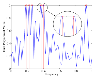
Figure 1: Frequency Localization using Dual Polynomial: The actual location of the frequencies in the line spectral signal $x^{\star}\in\mathbb{C}^{64}$ is shown in red. The blue curve is the dual polynomial obtained by solving (2) with $y=x^{\star}+w$ where $w$ is noise of SNR 10 dB.

As shown in Corollary 1, the dual solution can be used to identify the frequencies of the primal solution. For line spectra, a frequency $f\in[0,1]$ is in the support of the solution $\hat{x}$ of (1.1) if and only if

$$|\langle\hat{z},a_{f,\phi}\rangle|=\left|\ \sum_{l=0}^{n-1}\hat{z}_{l}e^{-i2\pi lf}\right|=\tau$$

That is, $f$ is in the support of $\hat{x}$ if and only if it is a point of maximum modulus for the dual polynomial. Thus, the support may be determined by finding frequencies $f$ where the dual polynomial attains magnitude $\tau$.

Figure 1 shows the dual polynomial for $\eqref{AST}$ with $n=64$ samples and $k=6$ randomly chosen frequencies. The regularization parameter $\tau$ is chosen as described in Section 3.2.

A recent result by Candes and Fernandez-Granda [26] establishes that in the noiseless case, the frequencies localized by the dual polynomial are exact provided the minimum separation between the frequencies is at least $4/n$ where $n$ is the number of samples in the line spectral signal. Under similar separation condition, numerical simulations suggest that (1.1) achieves approximate frequency location in the noisy case.

3.4 Discretization and Lasso

When the number of samples is larger than a few hundred, the running time of our ADMM method is dominated by the cost of computing eigenvalues and is usually expensive [38]. For very large problems, we now propose using Lasso as an alternative to the semidefinite program (3.4). To proceed, pick a uniform grid of $N$ frequencies and form $\mathcal{A}_{N}=\left\{a_{m/N,\phi}~{}\middle|~{}0\leq m\leq N-1\right\}\subset\mathcal{A}$ and solve (1.1) on this grid. i.e., we solve the problem

$$\text{minimize }\frac{1}{2}\lVert x-y\rVert_{2}^{2}+\tau\lVert x\rVert_{\mathcal{A}_{N}}.$$ (3.6)

To see why this is to our advantage, define $\Phi$ be the $n\times N$ Fourier matrix with $m$th column $a_{m/N,0}$. Then for any $x\in\mathbb{C}^{n}$ we have $\lVert x\rVert_{\mathcal{A}_{N}}=\min\left\{\lVert c\rVert_{1}:x=\Phi c\right\}$. So, we solve

$$\text{minimize }\frac{1}{2}\lVert\Phi c-y\rVert_{2}^{2}+\tau\lVert c\rVert_{1}.$$ (3.7)

for the optimal point $\hat{c}$ and set $\hat{x}_{N}=\Phi\hat{c}$ or the first $n$ terms of the $N$ term discrete Fourier transform (DFT) of $\hat{c}$. Furthermore, $\Phi^{*}z$ is simply the $N$ term inverse DFT of $z\in\mathbb{C}^{n}$. This observation coupled with Fast Fourier Transform (FFT) algorithm for efficiently computing DFTs gives a fast method to solve (3.6), using standard compressed sensing software for $\ell_{2}-\ell_{1}$ minimization, for example, SparSA [21].

Because of the relatively simple structure of the atomic set, the optimal solution $\hat{x}$ for (3.6) can be made arbitrarily close to (3.4) by picking $N$ a constant factor larger than $n$. In fact, we show that the atomic norms on $\mathcal{A}$ and $\mathcal{A}_{N}$ are equivalent (See Appendix C):

$$\left(1-\frac{2\pi n}{N}\right)\lVert x\rVert_{\mathcal{A}_{N}}\leq\lVert x\rVert_{\mathcal{A}}\leq\lVert x\rVert_{\mathcal{A}_{N}},\forall x\in\mathbb{C}^{n}$$ (3.8)

Using Proposition 3 and (3.5), we conclude

$$\frac{1}{n}\operatorname{\mathbb{E}}\lVert\hat{x}_{N}-x^{\star}\rVert_{2}^{2} \leq\frac{\sigma\left(\frac{\log(n)+1}{\log(n)}\right)\lVert x^{\star}\rVert_{\mathcal{A}}\sqrt{n\log(n)+n\log(4\pi\log(n))}}{n\left(1-\frac{2\pi n}{N}\right)}=O\left(\sigma\sqrt{\frac{\log(n)}{n}}\frac{\lVert x^{\star}\rVert_{\mathcal{A}}}{\left(1-\frac{2\pi n}{N}\right)}\right)$$

Due to the efficiency of the FFT, the discretized approach has a much lower algorithmic complexity than either Cadzow’s alternating projections method or the ADMM method described in Appendix E, which each require computing an eigenvalue decomposition at each iteration. Indeed, fast solvers for (3.7) converge to an $\epsilon$ optimal solution in no more than $1/\sqrt{\epsilon}$ iterations. Each iteration requires a multiplication by $\Phi$ and a simple “shrinkage” step. Multiplication by $\Phi$ or $\Phi^{*}$ requires $O(N\log N)$ time and the shrinkage operation can be performed in time $O(N)$.

As we discuss below, this fast form of basis pursuit has been proposed by several authors. However, analyzing this method with tools from compressed sensing has proven daunting because the matrix $\Phi$ is nowhere near a restricted isometry. Indeed, as $N$ tends to infinity, the columns become more and more coherent. However, common sense says that a larger grid should give better performance, for both denoising and frequency localization! Indeed, by appealing to the atomic norm framework, we are able to show exactly this point: the larger one makes $N$, the closer one approximates the desired atomic norm soft thresholding problem. Moreover, we do not have to choose $N$ to be too large in order to achieve nearly the same performance as the AST.

4 Related Work

The classical methods of line spectral estimation, often called linear prediction methods, are built upon the seminal interpolation method of Prony [39]. In the noiseless case, with as little as $n=2k$ measurements, Prony’s technique can identify the frequencies exactly, no matter how close the frequencies are. However, Prony’s technique is known to be sensitive to noise due to instability of polynomial rooting [40]. Following Prony, several methods have been employed to robustify polynomial rooting method including the Matrix Pencil algorithm [10], which recasts the polynomial rooting as a generalized eigenvalue problem and cleverly uses extra observations to guard against noise. The MUSIC [8] and ESPRIT [9] algorithms exploit the low rank structure of the autocorrelation matrix.

Cadzow [22] proposed a heuristic that improves over MUSIC by exploiting the Toeplitz structure of the matric of moments by alternately projecting between the linear space of Toeplitz matrices and the space of rank $k$ matrices where $k$ is the desired model order. Cadzow’s technique is very similar [41] to a popular technique in time series literature [42, 43] called Singular Spectrum Analysis [44], which uses autocorrelation matrix instead of the matrix of moments for projection. Both these techniques may be viewed as instances of structured low rank approximation [45] which exploit additional structure beyond low rank structure used in subspace based methods such as MUSIC and ESPRIT. Cadzow’s method has been identified as a fruitful preprocessing step for linear prediction methods [46]. A survey of classical linear prediction methods can be found in [46, 47] and an extensive list of references is given in [11].

Most, if not all of the linear prediction methods need to estimate the model order by employing some heuristic and the performance of the algorithm is sensitive to the model order. In contrast, our algorithms AST and the Lasso based method, only need a rough estimate of the noise variance. In our experiments, we provide the true model order to Matrix Pencil, MUSIC and Cadzow methods, while we use the estimate of noise variance for AST and Lasso methods, and still compare favorably to the classical line spectral methods.

In contrast to linear prediction methods, a number of authors  [23, 24, 25] have suggested using compressive sensing and viewing the frequency estimation as a sparse approximation problem. For instance, [24] notes that the Lasso based method has better empirical localization performance than the popular MUSIC algorithm. However, the theoretical analysis of this phenomenon is complicated because of the need to replace the continuous frequency space by an oversampled frequency grid. Compressive sensing based results (see, for instance, [48]) need to carefully control the incoherence of their linear maps to apply off-the-shelf tools from compressed sensing. It is important to note that the performance of our algorithm improves as the grid size increases. But this seems to contradict conventional wisdom in compressed sensing because our design matrix $\Phi$ becomes more and more coherent, and limits how fine we can grid for the theoretical guarantees to hold.

We circumvent the problems in the conventional compresssive sensing analysis by directly working in the continuous parameter space and hence step away from such notions as coherence, focussing on the geometry of the atomic set as the critical feature. By showing that the continuous approach is the limiting case of the Lasso based methods using the convergence of the corresponding atomic norms, we justify denoising line spectral signals using Lasso on a large grid. Since the original submission of this manuscript, Candès and Fernandez-Granda [26] showed that our SDP formulation exactly recovers the correct frequencies in the noiseless case.

5 Experiments

We compared the MSE performance of AST, the discretized Lasso approximation, the Matrix Pencil, MUSIC and Cadzow’s method. For our experiments, we generated $k$ normalized frequencies $f_{1}^{\star},\ldots,f_{k}^{\star}$ uniformly randomly chosen from $\left[0,1\right]$ such that every pair of frequencies are separated by at least $1/2n$. The signal $x^{\star}\in\mathbb{C}^{n}$ is generated according to (1.2) with $k$ random amplitudes independently chosen from $\chi^{2}(1)$ distribution (squared Gaussian). All of our sinusoids were then assigned a random phase (equivalent to multiplying $c_{k}^{\star}$ by a random unit norm complex number). Then, the observation $y$ is produced by adding complex white gaussian noise $w$ such that the input signal to noise ratio (SNR) is $-10,-5,0,5,10,15$ or $20$ dB. We compare the average MSE of the various algorithms in 10 trials for various values of number of observations $(n=64,128,256)$, and number of frequencies $(k=n/4,n/8,n/16)$.

AST needs an estimate of the noise variance $\sigma^{2}$ to pick the regularization parameter according to (3.5). In many situations, this variance is not known to us a priori. However, we can construct a reasonable estimate for $\sigma$ when the phases are uniformly random. It is known that the autocorrelation matrix of a line spectral signal (see, for example Chapter 4 in [47]) can be written as a sum of a low rank matrix and $\sigma^{2}I$ if we assume that the phases are uniformly random. Since the empirical autocorrelation matrix concentrates around the true expectation, we can estimate the noise variance by averaging a few smallest eigenvalues of the empirical autocorrelation matrix. In the following experiments, we form the empirical autocorrelation matrix using the MATLAB routine corrmtx using a prediction order $m=n/3$ and averaging the lower $25\%$ of the eigenvalues. We used this estimate in equation (3.5) to determine the regularization parameter for both our AST and Lasso experiments.

First, we implemented AST using the ADMM method described in detail in the Appendix. We used the stopping criteria described in [20] and set $\rho=2$ for all experiments. We use the dual solution $\hat{z}$ to determine the support of the optimal solution $\hat{x}$ using the procedure described in Section 3.3. Once the frequencies $\hat{f}_{l}$ are extracted, we ran the least squares problem $\mbox{minimize}_{\alpha}\|U\alpha-y\|^{2}$ where $U_{jl}=\exp(i2\pi j\hat{f}_{l})$ to obtain a debiased solution. After computing the optimal solution $\alpha_{\mathrm{opt}}$, we returned the prediction $\hat{x}=U\alpha_{\mathrm{opt}}$.

We implemented Lasso, obtaining an estimate $\hat{x}$ of $x^{\star}$ from $y$ by solving the optimization problem (3.6) with debiasing. We use the algorithm described in Section 3.4 with grid of $N=2^{m}$ points where $m=10,11,12,13,14$ and $15$. Because of the basis mismatch effect, the optimal $c_{\mathrm{opt}}$ has significantly more non-zero components than the true number of frequencies. However, we observe that the frequencies corresponding to the non-zero components of $c_{\mathrm{opt}}$ cluster around the true ones. We therefore extract one frequency from each cluster of non-zero values by identifying the grid point with the maximum absolute $c_{\mathrm{opt}}$ value and zero everything else in that cluster. We then ran a debiasing step which solves the least squares problem $\mbox{minimize}_{\beta}\|\Phi_{S}\beta-y\|^{2}$ where $\Phi_{S}$ is the submatrix of $\Phi$ whose columns correspond to frequencies identified from $c_{\mathrm{opt}}$. We return the estimate $\hat{x}=\Phi_{S}\beta_{\mathrm{opt}}$. We used the freely downloadable implementation of SpaRSA to solve the Lasso problem. We used a stopping parameter of $10^{-4}$, but otherwise used the default parameters.

We implemented Cadzow’s method as described by the pseudocode in [46], the Matrix Pencil as described in [10] and MUSIC [8] using the MATLAB routine rootmusic. All these algorithms need an estimate of the number of sinusoids. Rather than implementing a heuristic to estimate $k$, we fed the true $k$ to our solvers. This provides a huge advantage to these algorithms. Neither AST or the Lasso based algorithm are provided the true value of $k$, and the noise variance $\sigma^{2}$ required in the regularization parameter is estimated from $y$.

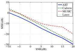
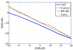
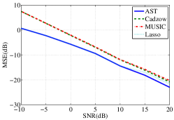
Figure 2: MSE vs SNR plots: This graph compares MSE vs SNR for a subset of experiments with $n=128$ samples. From left to right, the plots are for combinations of $8$, $16$, and $32$ sinusoids with amplitudes and frequencies sampled at random.

In Figure 2, we show MSE vs SNR plots for a subset of experiments when $n=128$ time samples are taken to take a closer look at the differences. It can be seen from these plots that the performance difference between classical algorithms such as MUSIC and Cadzow with respect to the convex optimization based AST and Lasso is most pronounced at lower sparsity levels. When the noise dominates the signal (SNR $\leq 0$ dB), all the algorithms are comparable. However, AST and Lasso outperform the other algorithms in almost every regime.

We note that the denoising performance of Lasso improves with increased grid size as shown in the MSE vs SNR plot in Figure 3(a). The figure shows that the performance improvement for larger grid sizes is greater at high SNRs. This is because when the noise is small, the discretization error is more dominant and finer gridding helps to reduce this error. Figures 3(a) and (b) also indicate that the benefits of increasing discretization levels are diminishing with the grid sizes, at a higher rate in the low SNR regime, suggesting a tradeoff among grid size, accuracy, and computational complexity.

Finally, in Figure 3(b), we provide numerical evidence supporting the assertion that frequency localization improves with increasing grid size. Lasso identifies more frequencies than the true ones due to basis mismatch. However, these frequencies cluster around the true ones, and more importantly, finer discretization improves clustering, suggesting over-discretization coupled with clustering and peak detection as a means for frequency localization for Lasso. This observation does not contradict the results of [49] where the authors look at the full Fourier basis ($N=n$) and the noise-free case. This is the situation where discretization effect is most prominent. We instead look at the scenario where $N\gg n$.

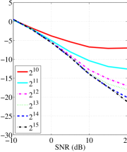
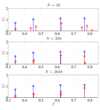
(a)	(b)

Figure 3: (a) Plot of MSE vs SNR for Lasso at different grid sizes for a subset of experiments with $n=128,k=16$. (b) Lasso Frequency localization with $n=32,k=4,$ SNR = $10$ dB. Blue represents the true frequencies, while red are given by Lasso. For better visualization, we threshold the Lasso solution by $10^{-6}$.

We use performance profiles to summarize the behavior of the various algorithms across all of the parameter settings. Performance profiles provide a good visual indicator of the relative performance of many algorithms under a variety of experimental conditions[50]. Let $\mathcal{P}$ be the set of experiments and let $\mathrm{MSE}_{s}(p)$ be the MSE of experiment $p\in\mathcal{P}$ using the algorithm $s$. Then the ordinate $P_{s}(\beta)$ of the graph at $\beta$ specifies the fraction of experiments where the ratio of the MSE of the algorithm $s$ to the minimum MSE across all algorithms for the given experiment is less than $\beta$, i.e.,

$$P_{s}(\beta)=\frac{\mathop{\#}\left\{p\in\mathcal{P}~{}:~{}\mathrm{MSE}_{s}(p)\leq\beta\min_{s}\mathrm{MSE}_{s}(p)\right\}}{\mathop{\#}(\mathcal{P})}$$

From the performance profile in Figure 4(a), we see that AST is the best performing algorithm, with Lasso coming in second. Cadzow does not perform as well as AST, even though it is fed the true number of sinusoids. When Cadzow is fed an incorrect $k$, even off by $1$, the performance degrades drastically, and never provides adequate mean-squared error. Figure 4(b) shows that the denoising performance improves with grid size.

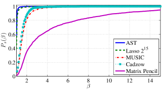
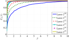
(a)	(b)

Figure 4: (a) Performance Profile comparing various algorithms and AST. (b) Performance profiles for Lasso with different grid sizes.

6 Conclusion and Future Work

The Atomic norm formulation of line spectral estimation provides several advantages over prior approaches. By performing the analysis in the continuous domain we were able to derive simple closed form rates using fairly straightforward techniques.We only grid the unit circle at the very end of our analysis and determine the loss incurred from discretization. This approach allowed us to circumvent some of the more complicated theoretical arguments that arise when using concepts from compressed sensing or random matrix theory.

This work provides several interesting possible future directions, both in line spectral estimation and in signal processing in general. We conclude with a short outline of some of the possibilities.

Fast Rates

Determining checkable conditions on the cones in Section 2.1 for the atomic norm problem is a major open problem. Our experiments suggest that when the frequencies are spread out, AST performs much better with a slightly larger regularization parameter. This observation was also made in the model-based compressed sensing literature [48]. Moreover, Candès and Fernandez Granda also needed a spread assumption to prove their theories.

This evidence together suggests the fast rate developed in Section 2.1 may be active for signals with well separated frequenies. Determining concrete conditions on the signal $x^{\star}$ that ensure this fast rate require techniques for estimating the parameter $\phi$ in (2.9). Such an investigation should be accompanied by a determination of the minimax rates for line spectral estimation. Such minimax rates would shed further light on the rates achievable for line spectral estimation.

Moments Supported Inside the Disk

Our work also naturally extends to moment problems where the atomic measures are supported on the unit disk in the complex plane. These problems arise naturally in controls and systems theory and include model order reduction, system identification, and control design. Applying the standard program developed in Section 2 provides a new look at these classic operator theory problems in control theory. It would be of significant importance to develop specialized atomic-norm denoising algorithms for control theoretic problems. Such an approach could yield novel statistical bounds for estimation of rational functions and $\mathcal{H}_{\infty}$-norm approximations.

Other Denoising Models

Our abstract denoising results in Section 2 apply to any atomic models and it is worth investigating their applicability for other models in statistical signal processing. For instance, it might be possible to pose a scheme for denoising a signal corrupted by multipath reflections. Here, the atoms might be all time and frequency shifted versions of some known signal. It remains to be seen what new insights in statistical signal processing can be gleaned from our unified approach to denoising.

Appendix A Optimality Conditions

A.0.1 Proof of Lemma 1

Proof.

The function $f(x)=\tfrac{1}{2}\lVert y-x\rVert_{2}^{2}+\tau\lVert x\rVert_{\mathcal{A}}$ is minimized at $\hat{x}$, if for all $\alpha\in(0,1)$ and all $x$,

$$f(\hat{x}+\alpha(x-\hat{x}))\geq f(\hat{x})$$

or equivalently,

$$\alpha^{-1}\tau\left(\lVert\hat{x}+\alpha(x-\hat{x})\rVert_{\mathcal{A}}-\lVert\hat{x}\rVert_{\mathcal{A}}\right)\geq\langle y-\hat{x},x-\hat{x}\rangle-\frac{1}{2}\alpha\lVert x-\hat{x}\rVert_{2}^{2}$$ (A.1)

Since $\lVert\cdot\rVert_{\mathcal{A}}$ is convex, we have

$$\lVert x\rVert_{\mathcal{A}}-\lVert\hat{x}\rVert_{\mathcal{A}}\geq\alpha^{-1}\left(\lVert\hat{x}+\alpha(x-\hat{x})\rVert_{\mathcal{A}}-\lVert\hat{x}\rVert_{\mathcal{A}}\right),$$

for all $x$ and for all $\alpha\in(0,1)$. Thus, by letting $\alpha\to 0$ in (A.1), we note that $\hat{x}$ minimizes $f(x)$ only if, for all $x$,

$$\tau\left(\lVert x\rVert_{\mathcal{A}}-\lVert\hat{x}\rVert_{\mathcal{A}}\right)\geq\langle y-\hat{x},x-\hat{x}\rangle.$$ (A.2)

However if (A.2) holds, then, for all $x$

$$\frac{1}{2}\|y-x\|_{2}^{2}+\tau\lVert x\rVert_{\mathcal{A}}\geq\frac{1}{2}\|y-\hat{x}+(\hat{x}-x)\|_{2}^{2}+\langle y-\hat{x},x-\hat{x}\rangle+\tau\lVert\hat{x}\rVert_{\mathcal{A}}$$

implying $f(x)\geq f(\hat{x}).$ Thus, (A.2) is necessary and sufficient for $\hat{x}$ to minimize $f(x)$.

Note.

The condition (A.2) simply says that $\tau^{-1}\left(y-\hat{x}\right)$ is in the subgradient of $\lVert\cdot\rVert_{\mathcal{A}}$ at $\hat{x}$ or equivalently that $0\in\partial f(\hat{x})$.

We can rewrite (A.2) as

$$\tau\lVert\hat{x}\rVert_{\mathcal{A}}-\langle y-\hat{x},\hat{x}\rangle\leq\inf_{x}\left\{\tau\lVert x\rVert_{\mathcal{A}}-\langle y-\hat{x},x\rangle\right\}$$ (A.3)

But by definition of the dual atomic norm,

$$\sup_{x}\left\{\langle z,x\rangle-\lVert x\rVert_{\mathcal{A}}\right\} =I_{\left\{w:\lVert w\rVert_{\mathcal{A}}^{*}\leq 1\right\}}(z)=\begin{cases}0&\lVert z\rVert_{\mathcal{A}}^{*}\leq 1\\ \infty&\text{otherwise.}\end{cases}$$ (A.4)

where $I_{A}(\cdot)$ is the convex indicator function. Using this in (A.3), we find that $\hat{x}$ is a minimizer if and only if $\lVert y-\hat{x}\rVert_{\mathcal{A}}^{*}\leq\tau$ and $\langle y-\hat{x},\hat{x}\rangle\geq\tau\lVert\hat{x}\rVert_{\mathcal{A}}$. This proves the theorem. ∎

A.0.2 Proof of Lemma 2

Proof.

We can rewrite the primal problem (1.1) as a constrained optimization problem:

$$\begin{split}&\mathop{\operatorname{minimize}}_{x,u}\frac{1}{2}\lVert y-x\rVert_{2}^{2}+\lVert u\rVert_{\mathcal{A}}\\ &\text{subject to }u=x.\end{split}$$

Now, we can introduce the Lagrangian function

$$L(x,u,z)=\frac{1}{2}\lVert y-x\rVert_{2}^{2}+\lVert u\rVert_{\mathcal{A}}+\langle z,x-u\rangle.$$

so that the dual function is given by

$$g(z)=\inf_{x,u}L(x,u,z) =\inf_{x}\left(\frac{1}{2}\lVert y-x\rVert_{2}^{2}+\langle z,x\rangle\right)+\inf_{u}\left(\tau\lVert u\rVert_{\mathcal{A}}-\langle z,u\rangle\right)$$

$$=\frac{1}{2}\left(\lVert y\rVert_{2}^{2}-\lVert y-z\rVert_{2}^{2}\right)-I_{\left\{w:\lVert w\rVert_{\mathcal{A}}^{*}\leq\tau\right\}}(z).$$

where the first infimum follows by completing the squares and the second infimum follows from (A.4). Thus the dual problem of maximizing $g(z)$ can be written as in (2).

The solution to the dual problem is the unique projection $\hat{z}$ of $y$ on to the closed convex set $C=\{z:\lVert z\rVert_{\mathcal{A}}^{*}\leq\tau\}$. By projection theorem for closed convex sets, $\hat{z}$ is a projection of $y$ onto $C$ if and only if $\hat{z}\in C$ and $\langle z-\hat{z},y-\hat{z}\rangle\leq 0$ for all $z\in C$, or equivalently if $\langle\hat{z},y-\hat{z}\rangle\geq\sup_{z}\,\langle z,y-\hat{z}\rangle=\tau\lVert y-\hat{z}\rVert_{\mathcal{A}}.$ These conditions are satisfied for $\hat{z}=y-\hat{x}$ where $\hat{x}$ minimizes $f(x)$ by Lemma 1. Now the proof follows by the substitution $\hat{z}=y-\hat{x}$ in the previous lemma. The absence of duality gap can be obtained by noting that the primal objective function at $\hat{x},$

$$f(\hat{x})=\frac{1}{2}\lVert y-\hat{x}\rVert_{2}^{2}+\langle\hat{z},\hat{x}\rangle=\frac{1}{2}\lVert\hat{z}\rVert_{2}^{2}+\langle\hat{z},\hat{x}\rangle=g(\hat{z}).$$

∎

Appendix B Fast Rate Calculations

We first prove the following

Proposition 4.

Let $\mathcal{A}=\{\pm e_{1},\ldots,\pm e_{n}\},$ be the set of signed canonical unit vectors in $\mathbb{R}^{n}$. Suppose $x^{\star}\in\mathbb{R}^{n}$ has $k$ nonzeros. Then $\phi_{\gamma}(x^{\star},\mathcal{A})\geq\frac{(1-\gamma)}{2\sqrt{k}}$.

Proof.

Let $z\in C_{\gamma}(x^{\star},\mathcal{A}).$ For some $\alpha>0$ we have,

$$\lVert x^{\star}+\alpha z\rVert_{1}\leq\lVert x^{\star}\rVert_{1}+\gamma\lVert\alpha z\rVert_{1}$$

In the above inequality, set $z=z_{T}+z_{T^{c}}$ where $z_{T}$ are the components on the support of $T$ and $z_{T^{c}}$ are the components on the complement of $T$. Since $x^{\star}+z_{T}$ and $z_{T^{c}}$ have disjoint supports, we have,

$$\lVert x^{\star}+\alpha z_{T}\rVert_{1}+\alpha\lVert z_{T^{c}}\rVert_{1}\leq\lVert x^{\star}\rVert_{1}+\gamma\lVert\alpha z_{T}\rVert_{1}+\gamma\lVert\alpha z_{T^{c}}\rVert_{1}\,.$$

This inequality implies

$$\lVert z_{T^{c}}\rVert_{1}\leq\frac{1+\gamma}{1-\gamma}\lVert z_{T}\rVert_{1}\,$$

that is, $z$ satisfies the null space property with a constant of $\tfrac{1+\gamma}{1-\gamma}.$ Thus,

$$\lVert z\rVert_{1}\leq\frac{2}{1-\gamma}\lVert z_{T}\rVert_{1}\leq\frac{2\sqrt{k}}{1-\gamma}\lVert z\rVert_{2}$$

This gives the desired lower bound. ∎

Now we can turn to the case of low rank matrices.

Proposition 5.

Let $\mathcal{A}$ be the manifold of unit norm rank-$1$ matrices in $\mathbb{C}^{n\times n}$. Suppose $X^{\star}\in\mathbb{C}^{n\times n}$ has rank $r$. Then $\phi_{\gamma}(X^{\star},\mathcal{A})\geq\frac{1-\gamma}{2\sqrt{2r}}$.

Proof.

Let $U\Sigma V^{H}$ be a singular value decomposition of $X^{\star}$ with $U\in\mathbb{C}^{n\times r}$, $V\in\mathbb{C}^{n\times r}$ and $\Sigma\in\mathbb{C}^{r\times r}$. Define the subspaces

$$T =\{UX+YV^{H}~{}:~{}X,Y\in\mathbb{C}^{n\times r}\}$$

$$T_{0} =\{UMV^{H}~{}:~{}M\in\mathbb{C}^{r\times r}\}$$

and let $\mathcal{P}_{T_{0}}$, $\mathcal{P}_{T}$, and $\mathcal{P}_{T^{\perp}}$ be projection operators that respectively map onto the subspaces $T_{0}$, $T$, and the orthogonal complement of $T$. Now, if $Z\in C_{\gamma}(X^{\star},\mathcal{A})$, then for some $\alpha>0$, we have

$$\lVert X^{\star}+\alpha Z\rVert_{*}\leq\lVert X^{\star}\rVert_{*}+\gamma\alpha\lVert Z\rVert_{*}\leq\lVert X^{\star}\rVert_{*}+\gamma\alpha\lVert\mathcal{P}_{T}(Z)\rVert_{*}+\gamma\alpha\lVert\mathcal{P}_{T^{\perp}}(Z)\rVert_{*}.$$ (B.1)

Now note that we have

$$\lVert X^{\star}+\alpha Z\rVert_{*}\geq\lVert X^{\star}+\alpha\mathcal{P}_{T_{0}}(Z)\rVert_{*}+\alpha\lVert\mathcal{P}_{T^{\perp}}(Z)\rVert_{*}$$

Substituting this in (B.1), we have,

$$\lVert X^{\star}+\alpha\mathcal{P}_{T_{0}}(Z)\rVert_{*}+\alpha\lVert\mathcal{P}_{T^{\perp}}(Z)\rVert_{*}\leq\lVert X^{\star}\rVert_{*}+\gamma\alpha\lVert\mathcal{P}_{T}(Z)\rVert_{*}+\gamma\alpha\lVert\mathcal{P}_{T^{\perp}}(Z)\rVert_{*}.$$

Since $\lVert\mathcal{P}_{T_{0}}(Z)\rVert_{*}\leq\lVert\mathcal{P}_{T}(Z)\rVert_{*}$, we have

$$\lVert\mathcal{P}_{T^{\perp}}(Z)\rVert_{*}\leq\frac{1+\gamma}{1-\gamma}\lVert\mathcal{P}_{T}(Z)\rVert_{*}.$$

Putting these computations together gives the estimate

$$\lVert Z\rVert_{*} \leq\lVert\mathcal{P}_{T}(Z)\rVert_{*}+\lVert\mathcal{P}_{T^{\perp}}(Z)\rVert_{*}\leq\frac{2}{1-\gamma}\lVert\mathcal{P}_{T}(Z)\rVert\leq\frac{2\sqrt{2r}}{1-\gamma}\lVert\mathcal{P}_{T}(Z)\rVert_{F}\leq\frac{2\sqrt{2r}}{1-\gamma}\lVert Z\rVert_{F}\,.$$

That is, we have $\phi_{\gamma}(X^{\star},\mathcal{A})\geq\frac{1-\gamma}{2\sqrt{2r}}$ as desired. ∎

Appendix C Approximation of the Dual Atomic Norm

This section furnishes the proof that the atomic norms induced by $\mathcal{A}$ and $\mathcal{A}_{N}$ are equivalent. Note that the dual atomic norm of $w$ is given by

$$\lVert w\rVert_{\mathcal{A}}^{*}=\sqrt{n}\sup_{f\in[0,1]}\left|W_{n}(e^{i2\pi f})\right|.$$ (C.1)

i.e., the maximum modulus of the polynomial $W_{n}$ defined by

$$W_{n}(e^{i2\pi f})=\frac{1}{\sqrt{n}}\sum_{m=0}^{n-1}{w_{m}e^{-i2\pi mf}}.$$ (C.2)

Treating $W_{n}$ as a function of $f$, with a slight abuse of notation, define

$$\lVert W_{n}\rVert_{\infty}:=\sup_{f\in[0,1]}\left|W_{n}(e^{i2\pi f})\right|.$$

We show that we can approximate the maximum modulus by evaluating $W_{n}$ in a uniform grid of $N$ points on the unit circle. To show that as $N$ becomes large, the approximation is close to the true value, we bound the derivative of $W_{n}$ using Bernstein’s inequality for polynomials.

Theorem 3 (Bernstein, See, for example  [51]).

Let $p_{n}$ be any polynomial of degree $n$ with complex coefficients. Then,

$$\sup_{|z|\leq 1}|p^{\prime}(z)|\leq n\sup_{|z|\leq 1}|p(z)|.$$

Note that for any $f_{1},f_{2}\in[0,1],$ we have

$$\left|W_{n}(e^{i2\pi f_{1}})\right|-\left|W_{n}(e^{i2\pi f_{2}})\right| \leq\left|e^{i2\pi f_{1}}-e^{i2\pi f_{2}}\right|\lVert W_{n}^{\prime}\rVert_{\infty}$$

$$=2|\sin(2\pi(f_{1}-f_{2}))|\lVert W_{n}^{\prime}\rVert_{\infty}$$

$$\leq 4\pi(f_{1}-f_{2})\lVert W_{n}^{\prime}\rVert_{\infty}$$

$$\leq 4\pi n(f_{1}-f_{2})\lVert W_{n}\rVert_{\infty},$$

where the last inequality follows by Bernstein’s theorem. Letting $s$ take any of the $N$ values $0,\tfrac{1}{N}\ldots,\tfrac{N-1}{N}$, we see that,

$$\lVert W_{n}\rVert_{\infty}\leq\max_{m=0,\ldots,N-1}\left|W_{n}\left(e^{i2\pi m/N}\right)\right|+\frac{2\pi n}{N}\lVert W_{n}\rVert_{\infty}.$$

Since the maximum on the grid is a lower bound for maximum modulus of $W_{n}$, we have

$$\max_{m=0,\ldots,N-1}\left|W_{n}\left(e^{i2\pi m/N}\right)\right|\leq\lVert W_{n}\rVert_{\infty}$$ (C.3)

$$\leq\left(1-\frac{2\pi n}{N}\right)^{-1}\max_{m=0,\ldots,N-1}\left|W_{n}\left(e^{i2\pi m/N}\right)\right|$$

$$\leq\left(1+\frac{4\pi n}{N}\right)\max_{m=0,\ldots,N-1}\left|W_{n}\left(e^{i2\pi m/N}\right)\right|.$$ (C.4)

Thus, for every $w,$

$$\lVert w\rVert_{\mathcal{A}_{N}}^{*}\leq\lVert w\rVert_{\mathcal{A}}^{*}\leq\left(1-\frac{2\pi n}{N}\right)^{-1}\lVert w\rVert_{\mathcal{A}_{N}}^{*}$$ (C.5)

or equivalently, for every $x,$

$$\left(1-\frac{2\pi n}{N}\right)\lVert x\rVert_{\mathcal{A}_{N}}\leq\lVert x\rVert_{\mathcal{A}}\leq\lVert x\rVert_{\mathcal{A}_{N}}$$ (C.6)

Appendix D Dual Atomic Norm Bounds

This section derives non-asymptotic upper and lower bounds on the expected dual norm of gaussian noise vectors, which are asymptotically tight upto $\log\log$ factors. Recall that the dual atomic norm of $w$ is given by $\sqrt{n}\sup_{f\in[0,1]}|W_{f}|$ where

$$W_{f}=\frac{1}{\sqrt{n}}\sum_{m=0}^{n-1}{w_{m}e^{-i2\pi mf}}.$$

The covariance function of $W_{f}$ is

$$\operatorname{\mathbb{E}}\left[W_{f_{1}}W_{f_{2}}^{*}\right] =\frac{1}{n}\sum_{m=0}^{n-1}\exp(2\pi m(f_{1}-f_{2}))=e^{\pi(n-1)(f_{1}-f_{2})}\frac{\sin(n\pi(f_{1}-f_{2}))}{n\sin(\pi(f_{2}-f_{2}))}.$$

Thus, the $n$ samples $\left\{W_{m/n}\right\}_{m=0}^{n-1}$ are uncorrelated and thus independent because of their joint gaussianity. This gives a simple non-asymptotic lower bound using the known result for maximum value of $n$ independent gaussian random variables [30] whenever $n>5$:

$$\operatorname{\mathbb{E}}\left[\sup_{t\in T}\left|W_{t}\right|\right] \geq\operatorname{\mathbb{E}}\left[\max_{m=0,\ldots,n-1}\mathop{\mathrm{Re}}\left(W_{m/n}\right)\right]=\sqrt{\log(n)-\tfrac{\log\log(n)+\log(4\pi)}{2}}.$$

We will show that the lower bound is asymptotically tight neglecting $\log\log$ terms. Since the dual norm induced by $\mathcal{A}_{N}$ approximates the dual norm induced by $\mathcal{A}$, (See C), it is sufficient to compute an upper bound for $\lVert w\rVert_{\mathcal{A}_{N}}^{*}.$ Note that $|W_{f}|^{2}$ has a chi-square distribution since $W_{f}$ is a Gaussian process. We establish a simple lemma about the maximum of chi-square distributed random variables.

Lemma 5.

Let $x_{1},\ldots,x_{N}$ be complex gaussians with unit variance. Then,

$$\operatorname{\mathbb{E}}\left[\max_{1\leq i\leq N}|x_{i}|\right]\leq\sqrt{\log(N)+1}.$$

Proof.

Let $x_{1},\ldots,x_{N}$ be complex Gaussians with unit variance: $\operatorname{\mathbb{E}}[|x_{i}|^{2}]=1$. Note that $2|x_{i}|^{2}$ is a chi-squared random variable with two degrees of freedom. Using Jensen’s inequality, also observe that

$$\operatorname{\mathbb{E}}\left[\max_{1\leq i\leq N}|x_{i}|\right] \leq\operatorname{\mathbb{E}}\left[\max_{1\leq i\leq N}|x_{i}|^{2}\right]^{1/2}\leq\tfrac{1}{\sqrt{2}}\operatorname{\mathbb{E}}\left[\max_{1\leq i\leq N}2|x_{i}|^{2}\right]^{1/2}.$$ (D.1)

Now let $z_{1},\ldots,z_{n}$ be chi-squared random variables with $2$ degrees of freedom. Then we have

$$\operatorname{\mathbb{E}}\left[\max_{1\leq i\leq N}z_{i}\right] =\int_{0}^{\infty}P\left[\max_{1\leq i\leq N}z_{i}\geq t\right]dt$$

$$\leq \delta+\int_{\delta}^{\infty}P\left[\max_{1\leq i\leq N}z_{i}\geq t\right]dt$$

$$\leq \delta+N\int_{\delta}^{\infty}P\left[z_{1}\geq t\right]dt$$

$$= \delta+N\int_{\delta}^{\infty}\exp(-t/2)dt$$

$$= \delta+2N\exp(-\delta/2)$$

Setting $\delta=2\log(N)$ gives $\operatorname{\mathbb{E}}\left[\max_{1\leq i\leq N}z_{i}\right]\leq 2\log{N}+2$. Plugging this estimate into (D.1) gives $\operatorname{\mathbb{E}}\left[\max_{1\leq i\leq N}|x_{i}|\right]\leq\sqrt{\log{N}+1}$. ∎

Using Lemma 5, we can compute

$$\lVert w\rVert_{\mathcal{A}_{N}}^{*} =\sqrt{n}\max_{m=0,\ldots,N-1}\left|W_{n}\left(e^{i2\pi m/N}\right)\right|\leq\sigma\sqrt{n\left(\log{N}+1\right)}$$

Plugging in $N=4\pi n\log(n)$ and using (C.1) and (C.4) establishes a tight upper bound.

Appendix E Alternating Direction Method of Multipliers for AST

A thorough survey of the ADMM algorithm is given in [20]. We only present the details essential to the implementation of atomic norm soft thresholding. To put our problem in an appropriate form for ADMM, rewrite (3.4) as

$$\begin{array}[]{ll}\operatorname*{minimize}_{t,u,x,Z}&\frac{1}{2}\|x-y\|_{2}^{2}+\frac{\tau}{2}(t+u_{1})\\ \operatorname{subject\ to}&Z=\begin{bmatrix}T(u)&x\\ x^{*}&t\end{bmatrix}\\ &Z\succeq 0.\end{array}$$

and dualize the equality constraint via an Augmented Lagrangian:

$$\mathcal{L}_{\rho}(t,u,x,Z,\Lambda)=\frac{1}{2}\|x-y\|_{2}^{2}+\frac{\tau}{2}(t+u_{1})+$$

$$\left\langle\Lambda,Z-\begin{bmatrix}T(u)&x\\ x^{*}&t\end{bmatrix}\right\rangle+\frac{\rho}{2}\left\|Z-\begin{bmatrix}T(u)&x\\ x^{*}&t\end{bmatrix}\right\|_{F}^{2}$$

ADMM then consists of the update steps:

$$(t^{l+1},u^{l+1},x^{l+1})\leftarrow\arg\min_{t,u,x}\mathcal{L}_{\rho}(t,u,x,Z^{l},\Lambda^{l})$$

$$Z^{l+1}\leftarrow\arg\min_{Z\succeq 0}\mathcal{L}_{\rho}(t^{l+1},u^{l+1},x^{l+1},Z,\Lambda^{l})$$

$$\Lambda^{l+1}\leftarrow\Lambda^{l}+\rho\left(Z^{l+1}-\begin{bmatrix}T(u^{l+1})&x^{l+1}\\ {x^{l+1}}^{*}&t^{l+1}\end{bmatrix}\right).$$

The updates with respect to $t$, $x$, and $u$ can be computed in closed form:

$$t^{l+1} =Z_{n+1,n+1}^{l}+\left(\Lambda_{n+1,n+1}^{l}-\frac{\tau}{2}\right)/\rho$$

$$x^{l+1} =\frac{1}{2\rho+1}(y+2\rho z_{1}^{l}+2\lambda_{1}^{l})$$

$$u^{l+1} =W\left(T^{*}(Z_{0}^{l}+\Lambda_{0}^{l}/\rho)-\frac{\tau}{2\rho}{e}_{1}\right)$$

Here $W$ is the diagonal matrix with entries

$$W_{ii}=\begin{cases}\frac{1}{n}&i=1\\ \frac{1}{2(n-i+1)}&i>1\end{cases}$$

and we introduced the partitions:

$$Z^{l}=\begin{bmatrix}Z_{0}^{l}&z_{1}^{l}\\ {z_{1}^{l}}^{*}&Z^{l}_{n+1,n+1}\end{bmatrix}~{}~{}~{}\mbox{and}~{}~{}~{}\Lambda^{l}=\begin{bmatrix}\Lambda_{0}^{l}&\lambda_{1}^{l}\\ {\lambda_{1}^{l}}^{*}&\Lambda^{l}_{n+1,n+1}\end{bmatrix}\,.$$

The $Z$ update is simply the projection onto the positive definite cone

$$Z^{l+1}:=\arg\min_{Z\succeq 0}\left\|Z-\begin{bmatrix}T(u^{l+1})&x^{l+1}\\ {x^{l+1}}^{*}&t^{l+1}\end{bmatrix}+\Lambda^{l}/\rho\right\|_{F}^{2}\,.$$ (E.1)

Projecting a matrix $Q$ onto the positive definite cone is accomplished by forming an eigenvalue decomposition of $Q$ and setting all negative eigenvalues to zero.

To summarize, the update for $(t,u,x)$ requires averaging the diagonals of a matrix (which is equivalent to projecting a matrix onto the space of Toeplitz matrices), and hence operations that are $O(n)$. The update for $Z$ requires projecting onto the positive definite cone and requires $O(n^{3})$ operations. The update for $\Lambda$ is simply addition of symmetric matrices.

Note that the dual solution $\hat{z}$ can be obtained as $\hat{z}=y-\hat{x}$ from the primal solution $\hat{x}$ obtained from ADMM by using Lemma 2.

References

- [1] R. Carriere and R. Moses, “High resolution radar target modeling using a modified Prony estimator,” IEEE Trans. on Antennas and Propagation, vol. 40, no. 1, pp. 13–18, 1992.
- [2] H. Krim and M. Viberg, “Two decades of array signal processing research: the parametric approach,” IEEE Signal Processing Magazine, vol. 13, no. 4, pp. 67–94, 1996.
- [3] L. Borcea, G. Papanicolaou, C. Tsogka, and J. Berryman, “Imaging and time reversal in random media,” Inverse Problems, vol. 18, p. 1247, 2002.
- [4] I. Maravic, J. Kusuma, and M. Vetterli, “Low-sampling rate UWB channel characterization and synchronization,” Journal of Communications and Networks, vol. 5, no. 4, pp. 319–327, 2003.
- [5] V. Viti, C. Petrucci, and P. Barone, “Prony methods in NMR spectroscopy,” Intl. Journal of Imaging Systems and Technology, vol. 8, no. 6, pp. 565–571, 1997.
- [6] X. Andrade, J. Sanders, and A. Aspuru-Guzik, “Application of compressed sensing to the simulation of atomic systems,” Proc. of the National Academy of Sciences, vol. 109, no. 35, pp. 13928–13933, 2012.
- [7] Z. Leonowicz, T. Lobos, and J. Rezmer, “Advanced spectrum estimation methods for signal analysis in power electronics,” IEEE Trans. on Industrial Electronics, vol. 50, pp. 514 – 519, june 2003.
- [8] R. Schmidt, “Multiple emitter location and signal parameter estimation,” IEEE Trans. on Antennas and Propagation, vol. 34, no. 3, pp. 276–280, 1986.
- [9] R. Roy and T. Kailath, “ESPRIT - estimation of signal parameters via rotational invariance techniques,” IEEE Trans. on Acoustics, Speech and Signal Processing, vol. 37, no. 7, pp. 984–995, 1989.
- [10] Y. Hua and T. Sarkar, “Matrix pencil method for estimating parameters of exponentially damped/undamped sinusoids in noise,” IEEE Trans. on Acoustics, Speech and Signal Processing, vol. 38, no. 5, pp. 814–824, 1990.
- [11] P. Stoica, “List of references on spectral line analysis,” Signal Processing, vol. 31, no. 3, pp. 329–340, 1993.
- [12] V. Chandrasekaran, B. Recht, P. Parrilo, and A. Willsky, “The convex geometry of linear inverse problems,” Arxiv preprint arXiv:1012.0621, December 2010.
- [13] E. Candès, J. Rombergh, and T. Tao, “Stable signal recovery from incomplete and inaccurate measurements,” Comm. on Pure and Applied Mathematics, vol. 59, no. 8, pp. 1207–1223, 2006.
- [14] B. Recht, M. Fazel, and P. Parrilo, “Guaranteed minimum rank solutions of matrix equations via nuclear norm minimization,” SIAM Review, vol. 52, no. 3, pp. 471–501, 2010.
- [15] E. Candès and B. Recht, “Exact matrix completion via convex optimization,” Foundations of Computational Mathematics, vol. 9, no. 6, pp. 717–772, 2009.
- [16] R. Tibshirani, “Regression shrinkage and selection via the lasso,” Journal of the Royal Statistical Society. Series B, vol. 58, no. 1, pp. 267–288, 1996.
- [17] S. Chen, D. Donoho, and M. Saunders, “Atomic decomposition by basis pursuit,” SIAM Review, vol. 43, pp. 129–159, 2001.
- [18] A. Megretski, “Positivity of trigonometric polynomials,” in Proc. 42nd IEEE Conference on Decision and Control, vol. 4, pp. 3814–3817, 2003.
- [19] D. P. Bertsekas and J. N. Tsitsiklis, Parallel and Distributed Computation: Numerical Methods. Belmont, MA: Athena Scientific, 1997.
- [20] S. Boyd, N. Parikh, B. P. E. Chu, and J. Eckstein, “Distributed optimization and statistical learning via the alternating direction method of multipliers,” Foundations and Trends in Machine Learning, vol. 3, pp. 1–122, December 2011.
- [21] S. J. Wright, R. D. Nowak, and M. A. T. Figueiredo, “Sparse reconstruction by separable approximation,” IEEE Trans. on Signal Processing, vol. 57, no. 7, pp. 2479–2493, 2009.
- [22] J. Cadzow, “Signal enhancement-a composite property mapping algorithm,” IEEE Trans. on Acoustics, Speech and Signal Processing, vol. 36, no. 1, pp. 49–62, 1988.
- [23] S. Chen and D. Donoho, “Application of basis pursuit in spectrum estimation,” in Proc. IEEE Intl. Conference on Acoustics, Speech and Signal Processing, vol. 3, pp. 1865–1868, IEEE, 1998.
- [24] D. Malioutov, M. Çetin, and A. Willsky, “A sparse signal reconstruction perspective for source localization with sensor arrays,” IEEE Trans. on Signal Processing, vol. 53, no. 8, pp. 3010–3022, 2005.
- [25] S. Bourguignon, H. Carfantan, and J. Idier, “A sparsity-based method for the estimation of spectral lines from irregularly sampled data,” IEEE Journal of Selected Topics in Signal Processing, vol. 1, no. 4, pp. 575–585, 2007.
- [26] E. Candes and C. Fernandez-Granda, “Towards a mathematical theory of super-resolution,” arXiv Preprint 1203.5871, 2012.
- [27] G. Tang, B. Bhaskar, P. Shah, and B. Recht, “Compressed sensing off the grid,” arXiv Preprint 1207.6053, 2012.
- [28] B. K. Natarajan, “Sparse approximate solutions to linear systems,” SIAM Journal of Computing, vol. 24, no. 2, pp. 227–234, 1995.
- [29] D. Donoho, “De-noising by soft-thresholding,” IEEE Trans. on Information Theory, vol. 41, no. 3, pp. 613–627, 1995.
- [30] T. Lai and H. Robbins, “Maximally dependent random variables,” Proc. of the National Academy of Sciences, vol. 73, no. 2, p. 286, 1976.
- [31] E. Greenshtein and Y. Ritov, “Persistence in high-dimensional linear predictor selection and the virtue of overparametrization,” Bernoulli, vol. 10, no. 6, pp. 971–988, 2004.
- [32] S. van de Geer and P. Bühlmann, “On the conditions used to prove oracle results for the lasso,” Electronic Journal of Statistics, vol. 3, pp. 1360–1392, 2009.
- [33] D. L. Donoho and I. M. Johnstone, “Ideal spatial adaptation by wavelet shrinkage,” Biometrika, vol. 81, no. 3, pp. 425–455, 1994.
- [34] K. R. Davidson and S. J. Szarek, “Local operator theory, random matrices and Banach spaces,” in Handbook on the Geometry of Banach spaces (W. B. Johnson and J. Lindenstrauss, eds.), pp. 317–366, Elsevier Scientific, 2001.
- [35] B. A. Dumitrescu, Positive Trigonometric Polynomials and Signal Processing Applications. Netherlands: Springer, 2007.
- [36] J. F. Sturm, “Using SeDuMi 1.02, a MATLAB toolbox for optimization over symmetric cones,” Optimization Methods and Software, vol. 11-12, pp. 625–653, 1999.
- [37] K. C. Toh, M. Todd, and R. H. Tütüncü, SDPT3: A MATLAB software package for semidefinite-quadratic-linear programming. Available from http://www.math.nus.edu.sg/~mattohkc/sdpt3.html.
- [38] B. N. Bhaskar, G. Tang, and B. Recht, “Atomic norm denoising with applications to line spectral estimation,” tech. rep., 2012. Extended Technical Report. Available at arxiv.org/1204.0562.
- [39] R. Prony, “Essai experimental et analytique,” J. Ec. Polytech.(Paris), vol. 2, pp. 24–76, 1795.
- [40] M. Kahn, M. Mackisack, M. Osborne, and G. Smyth, “On the consistency of Prony’s method and related algorithms,” Journal of Computational and Graphical Statistics, vol. 1, no. 4, pp. 329–349, 1992.
- [41] A. Zhigljavsky, “Singular spectrum analysis for time series: Introduction to this special issue,” Statistics and its Interface, vol. 3, no. 3, pp. 255–258, 2010.
- [42] H. Kantz and T. Schreiber, Nonlinear time series analysis, vol. 7. Cambridge University Press, 2003.
- [43] N. Golyandina, V. Nekrutkin, and A. Zhigljavsky, Analysis of Time Series Structure: SSA and related techniques, vol. 90. Chapman & Hall/CRC, 2001.
- [44] R. Vautard, P. Yiou, and M. Ghil, “Singular-spectrum analysis: A toolkit for short, noisy chaotic signals,” Physica D: Nonlinear Phenomena, vol. 58, no. 1, pp. 95–126, 1992.
- [45] M. Chu, R. Funderlic, and R. Plemmons, “Structured low rank approximation,” Linear algebra and its applications, vol. 366, pp. 157–172, 2003.
- [46] T. Blu, P. Dragotti, M. Vetterli, P. Marziliano, and L. Coulot, “Sparse sampling of signal innovations,” IEEE Signal Processing Magazine, vol. 25, no. 2, pp. 31–40, 2008.
- [47] P. Stoica and R. Moses, Spectral analysis of signals. Pearson/Prentice Hall, 2005.
- [48] M. Duarte and R. Baraniuk, “Spectral compressive sensing,” Applied and Computational Harmonic Analysis, 2012.
- [49] Y. Chi, L. Scharf, A. Pezeshki, and A. Calderbank, “Sensitivity to basis mismatch in compressed sensing,” Signal Processing, IEEE Transactions on, vol. 59, no. 5, pp. 2182–2195, 2011.
- [50] E. Dolan and J. Moré, “Benchmarking optimization software with performance profiles,” Mathematical Programming, vol. 91, no. 2, pp. 201–213, 2002.
- [51] A. Schaeffer, “Inequalities of A. Markoff and S. Bernstein for polynomials and related functions,” Bull. Amer. Math. Soc, vol. 47, pp. 565–579, 1941.