A young stellar cluster within the RCW41 Hii region: deep NIR photometry and Optical/NIR polarimetry^⋆

Abstract

The RCW41 star-forming region is embedded within the Vela Molecular Ridge, hosting a massive stellar cluster surrounded by a conspicuous Hii region. Understanding the role of interstellar magnetic fields and studying the newborn stellar population is crucial to build a consistent picture of the physical processes acting on this kind of environment. We have carried out a detailed study of the interstellar polarization toward RCW41, with data from an optical and near-infrared polarimetric survey. Additionally, deep near-infrared images from the NTT 3.5 m telescope have been used to study the photometric properties of the embedded young stellar cluster, revealing several YSO’s candidates. By using a set of pre-main sequence isochrones, a mean cluster age in the range 2.5 - 5.0 million years was determined, and evidence of sequential star formation were revealed. An abrupt decrease in R-band polarization degree is noticed toward the central ionized area, probably due to low grain alignment efficiency caused by the turbulent environment and/or weak intensity of magnetic fields. The distortion of magnetic field lines exhibit a dual behavior, with the mean orientation outside the area approximately following the borders of the star-forming region, and directed radially toward the cluster inside the ionized area, in agreement with simulations of expanding Hii regions. The spectral dependence of polarization allowed a meaningful determination of the total-to-selective extinction ratio by fittings of the Serkowski relation. Furthermore, a large rotation of polarization angle as a function of wavelength is detected toward several embedded stars.

1. Introduction

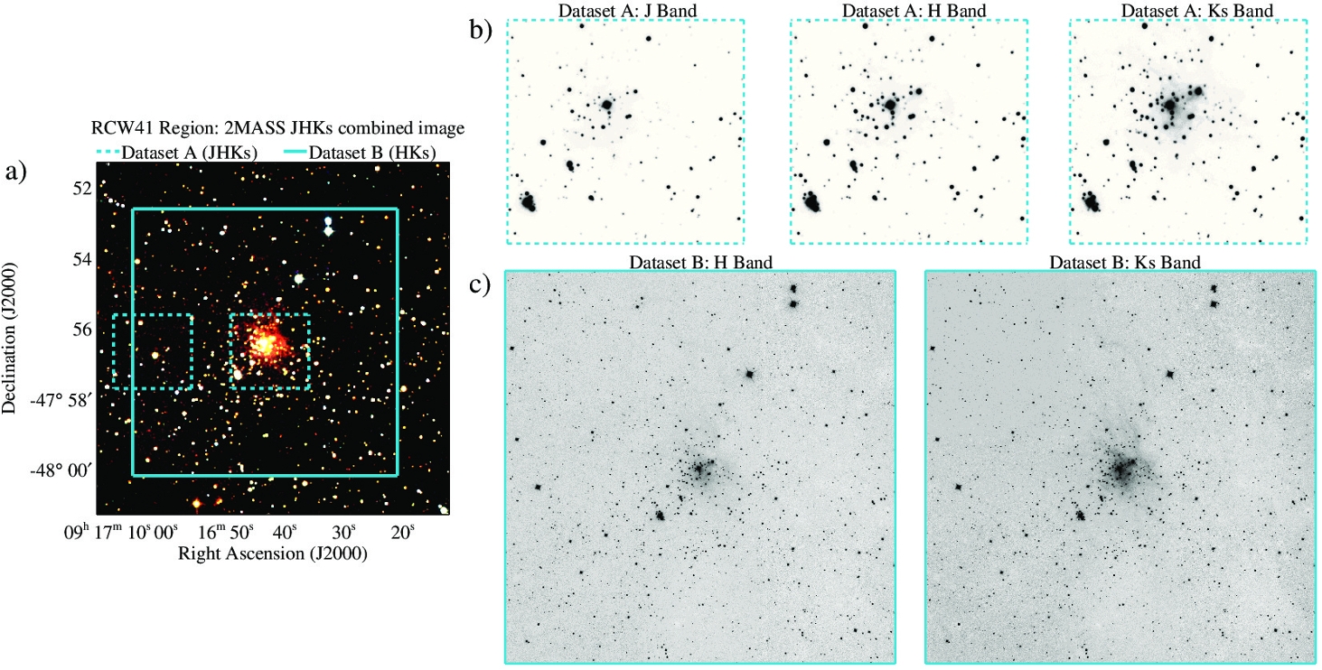
Figure 1.— (a) Composite JHKs image (RGB) from the 2MASS survey showing the cluster in the direction of the IRAS 09149-4743 source, as well as the regions associated to our NIR photometry datasets: the dashed-line cyan rectangles indicates the regions related to Dataset A (J, H and Ks filters) and the solid-line cyan rectangle is related to Dataset B (H and Ks filters). (b) Images of the cluster region from Dataset A, at filters J (left), H (middle) and Ks (right). (c) Mosaics of the entire region of RCW41 covered by Dataset B at H (left) and Ks (right) filters.

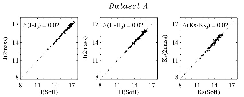
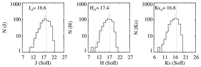
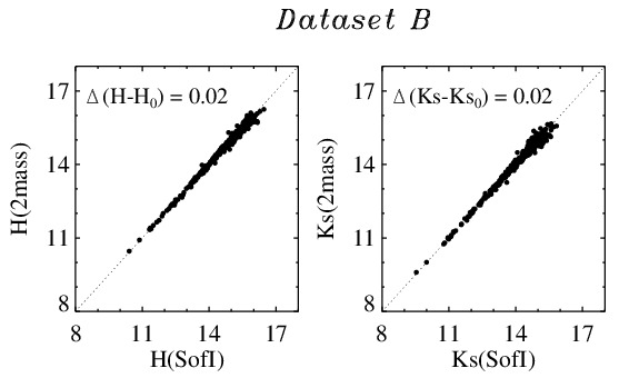
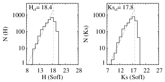
Figure 2.— Comparison between SofI and 2MASS magnitudes as well as magnitude histograms used to derive the completeness limits, shown above for Dataset A (J, H and Ks filters) and below for Dataset B (H and Ks filters). The comparison diagrams were used to determine the zero point corrections for each filter, and the respective zero point uncertainties are indicated inside each diagram. The dashed lines represents the ideal correspondence between the two systems, and were inserted in order to clarify the comparison. Only isolated and good quality photometry stars (flag “A”) from the 2MASS catalog were used. The magnitude histograms were used to calculate the completeness limits (cl) to each filter from Datasets A and B, and are indicated by the vertical dashed lines.

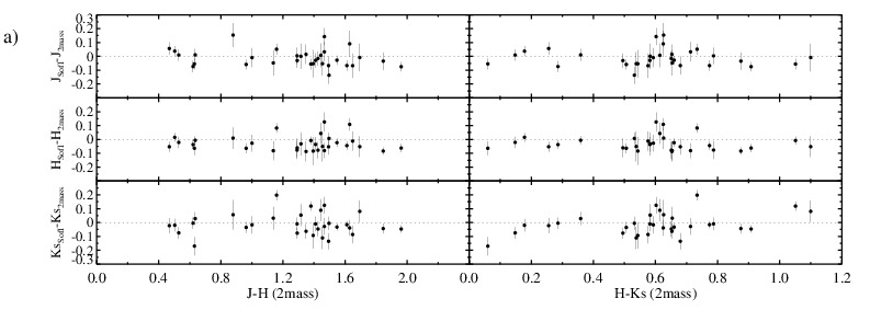
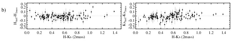
Figure 3.— Diagrams related to Datasets A (a) and B (b), used to verify a possible color dependence associated to the photometric calibration of the SofI magnitudes based on the 2MASS magnitudes. The horizontal dashed lines were inserted for clarity. The dispersion shows that no presence of color dependences are evident within our instrumental uncertainties.

It is well known that sites of massive star formation are mainly found inside heavily obscured dusty molecular cores, which are commonly associated to giant molecular cloud complexes (e.g., Lada & Lada, 2003; Lada, 2010). Photometric studies at near-infrared (NIR) wavelengths make possible to probe deep inside where star formation is taking place, with the very young stars frequently showing large infrared excesses due to the presence of warm dust from the associated circumstellar disks.

On the other hand, the study of the interstellar dust grain’s interaction with the local magnetic fields, is a powerful tool to understand some of the physical processes acting in such environments. In this context, magnetic fields might play a key role in star formation. In fact, several physical processes, like the initial cloud collapse by the fragmentation of early stage star-forming cores, the channeling of interstellar material via ambipolar diffusion, the disk and bipolar outflow formation, the angular momentum transport, etc, possibly are strongly affected by the strength and configuration of the local magnetic field components (Mestel & Spitzer, 1956; Nakano, 1979; Mouschovias & Paleologou, 1981; Shu et al., 1987; Lizano & Shu, 1989; Heitsch et al., 2004; Girart et al., 2009). However, it is still unknown whether magnetic fields or interstellar turbulence provide the main supporting source against the cloud collapse, ultimately defining the star formation efficiency (Padoan et al., 2004; Crutcher, 2005; Heiles & Crutcher, 2005; McKee & Ostriker, 2007).

The formation of massive stars causes a large impact on the surrounding environment, ionizing the interstellar gas and providing a source of turbulence due to strong stellar winds and outflows from the newborn stellar population. Only recently, theoretical studies have attempted to describe a realistic view of the impact of the expansion of Hii regions on the underlying structures of the magnetic field lines (Krumholz et al., 2007; Peters et al., 2010, 2011; Arthur et al., 2011). Unfortunately, mappings of the magnetic field structures along the majority of Galactic Hii regions are scarcely available, although these could serve as important tests and provide additional constraints to such models of star formation.

An important method to map the sky-projected lines of magnetic field using optical or NIR spectral bands, is from interstellar polarization by aligned dust grains, that serves as a well known tracer. A detailed study of linear polarization toward Hii regions and young stellar clusters can provide useful information regarding the structure of the Galactic magnetic field in these regions.

The Vela Molecular Ridge (VMR) is an interesting Galactic complex where star formation is taking place over a wide range of masses (Liseau et al., 1992; Lorenzetti et al., 1993; Massi et al., 1999, 2000, 2003). It is located at the Galactic Plane roughly towards $l\sim 265^{\circ}$, where one can see the presence of several large interstellar features, such as the Vela supernova remnant, the Gum Nebula, and other structures. Beyond this “local” structure, at the $1-2$ kpc range, several young star clusters are found, as well as numerous optical Hii regions with several signposts of embedded star formation such as H₂O masers (Braz & Epchtein, 1983; Zinchenko et al., 1995).

Among these structures, a giant molecular complex extends over $20^{\circ}$ in the southern sky. It can be identified by its strong CO emission, and was first studied by Murphy & May (1991), who divided the main structure into four regions, named $A$ to $D$. Clouds towards these areas are located along a wide range of distances, from $700$ to $\sim 2000$ pc (Liseau et al., 1992). According to Murphy & May (1991) regions $A$, $C$ and $D$ are located quite closer to us ($\sim 1$kpc), with the cloud $B$ being slightly more distant ($\sim 2$kpc). Recently, a submillimetric survey carried out by Olmi et al. (2009) detected approximately 140 proto- and pre-stellar cores in the direction of cloud $D$.

The IRAS 09149-4743 source is an example of young stellar cluster in this region. It is part of the cloud $A$, being located at an estimated distance of $1.3\pm 0.2$ kpc (Roman-Lopes et al., 2009). It shows several candidate young stellar objects (YSOs), as well as, two massive stars of spectral types O9v and B0v, as revealed by previous photometric and spectroscopic infrared surveys (Ortiz et al., 2007; Roman-Lopes et al., 2009). Several radio and infrared observations are available in the direction of IRAS 09149-4743, tracing a number of chemical elements in this region, which are mainly related to the existence of the surrounding Hii region and the massive star forming area. Ortiz et al. (2007) compiled a list of all observational data collected from the literature up to that date. Furthermore, Pirogov et al. (2007) reported the detection of CS, N₂H⁺ and 1.2 mm dust continuum emissions toward IRAS 09149-4743. Specifically, the dust emission represent an almost spherical core approximately superposed to the stellar cluster direction. Pirogov (2009) carried out further studies of these data through analysis of the cloud’s radial density profile.

Our main goal in this work is to study the stellar population of the associated massive star cluster, as well as, to investigate the structure of the interstellar magnetic field in the direction of the related Hii region. This was done by combining new deep NIR imaging with optical and NIR polarimetric data of the related region. The paper is organized as follow: Section 2 describes the NIR photometric data and reduction techniques, as well as, the polarimetric observational sample. Results and analysis obtained from the photometric and polarimetric data are separately exposed respectively in Sections 3 and 4. Discussion of these results are introduced in Section 5, and the final conclusions are listed in Section 6.

2. Observational Data

2.1. Near-Infrared Photometry

The raw imaging data for the IRAS 09149-4743 region were retrieved from the ESO archive, and the observations comprise two separate programs with the following identifiers: 073.D-0102 (PI Dr. Sergio Ortolani) and 080.D-0470 (PI Dr. Ben Davies). The observing missions were conducted during the nights of May 5th 2004 and February 10th 2008 using the SofI (“Son of Isaac”) NIR camera (Moorwood et al., 1998), mounted on the NTT 3.58 m telescope from La Silla/Chile.

In Figure 1a we use a combined 2MASS (Skrutskie et al., 2006) image of the studied region to show the surveyed area. The 2004 survey corresponds to the two small squares shown in this figure (delimited by cyan dashed lines); one centered on the stellar cluster and the other on a nearby control field. This survey will be hereafter denominated “Dataset A”, and corresponds to J, H and Ks bands observations using a $0.144^{\prime\prime}$/pixel plate scale, which allows a $2.1\mathrm{{}^{\prime}}\times 2.1\mathrm{{}^{\prime}}$ field-of-view. The observational strategy included 24 expositions at each of the three filters, corresponding to 12 observations of the cluster field intercalated with 12 observations of the control field. Moreover, successive observations of the same field were made by jittering the telescope by a small displacement ($\approx 9.5^{\prime\prime}$, roughly in the NE-SW direction) between each exposition. The FWHM values of point-like sources at this observational run are of $\approx 1$”.

The observational data from the 2008 survey (which we hereafter denominate “Dataset B”) was obtained using the H and Ks bands, with a plate scale of $0.288^{\prime\prime}$/pixel, allowing a field of view of about $4.9\mathrm{{}^{\prime}}\times 4.9\mathrm{{}^{\prime}}$. Four jittering positions were used, moving the telescope in the N-E-S-W directions while positioning the cluster in each of the four quarters of the frame. Using this method, a larger field could be mapped covering an area of $7.4\mathrm{{}^{\prime}}\times 7.4\mathrm{{}^{\prime}}$ on the sky, centered on the stellar cluster. In Figure 1a the region associated to Dataset B corresponds to the larger square delimited by a solid line. Atmospheric conditions during this observational run allowed mean FWHM values of $\approx 0.7$”.

Images from both datasets were treated by using IRAF(Tody, 1986) tasks from the NOAO package to perform the following reduction steps: division by a flat-field frame and illumination pattern, correction of bad pixels from the frame using a bad pixel mask, correction of the “crosstalk effect”, combination of jittered images in order to create sky fields, subtraction of the sky images, combination of the sky-subtracted images and alignment of images from different filters. The reduced images of Datasets A and B are respectively displayed on Figures 1b and 1c. MONTAGE was used to create the $7.4\mathrm{{}^{\prime}}\times 7.4\mathrm{{}^{\prime}}$ field mosaic of Dataset B (Figure 1c).

DAOFIND (from the DAOPHOT package) was used to locate stars peaked with $3\sigma$ above the background, and objects missed by this routine were further inserted by visual inspection. Astrometric configuration of the objects’ world coordinate system was done by using a sample of 2MASS isolated objects from the same field. Correction of the coordinates was achieved with a rms uncertainty of $\approx 0.05$ arcsec in right ascencion ($\alpha$) and declination ($\delta$), for both Datasets.

PSF photometry was further performed using the algorithms from the DAOPHOT package (Stetson, 1987), with the following photometric parameters for each Dataset: PSF radius of $2.30^{\prime\prime}$ and fitting radius of $1.30^{\prime\prime}$ for Dataset A; PSF radius of $2.59^{\prime\prime}$ and fitting radius of $0.86^{\prime\prime}$ for Dataset B. Several runs of psf fitting and stellar subtraction were performed in order to reveal and obtain magnitudes for the very close faint companions from the most crowded areas.

Photometric calibration was achieved by comparing the instrumental magnitudes with a sample of isolated, good quality photometry stars (flag “A”) at the same field from the 2MASS survey. Such comparison is shown in Figure 2 for both datasets. These diagrams show a quite good correlation, with zero point uncertainties of $0.02$ mag in all photometric bands for both datasets. Individual magnitude uncertainties were computed using a quadratic sum of the instrumental errors from the psf photometry and the calibration uncertainty.

Furthermore, approximate completeness limits were derived from the analysis of the histograms, also shown in Figure 2. It is defined as the point where the histograms deviate from the straight line, which represent a linear fit to the logarithmic of the number of objects per magnitude bin. The values obtained for Datasets A and B are $(\mathrm{J},\mathrm{H},\mathrm{Ks})_{limit}=(18.6,17.4,16.8)$ and $(\mathrm{H},\mathrm{Ks})_{limit}=(18.4,17.8)$, respectively. Considering the above photometric limits of both datasets, an improvement of 1.6, 2.1 and 2.8 magnitudes have been obtained respectively in J, H and Ks bands, as compared to the earlier survey by Ortiz et al. (2007), allowing us to probe deeper into the lower-mass stellar population.

In order to check the existence of color dependence terms to be applied to the SOFI photometry, we constructed diagrams of magnitude differences (between the SofI and 2MASS systems) as a function of the (J-H) and (H-Ks) colors, as can be seen on Figures 3a (Dataset A) and 3b (Dataset B, only the H-Ks color). As can be noticed, there is no need to apply color correction terms to the derived SOFI photometry.

The photometric results are shown in the Appendix, respectively corresponding to 530 and 2608 stars in Datasets A (Table 1) and B (Table 2). The full versions of the tables are available only in the electronic version of this paper.

2.2. Optical/Near-Infrared Polarimetry

The optical and NIR polarimetric data used in this work have been separately obtained with different telescopes and instrumental configurations. The optical data were collected using the 0.9 m telescope of the CTIO (Cerro Tololo, Chile, operated by the National Optical Astronomy Observatory - NOAO) observatory, during February and April/2010; and March/2011. The NIR data were obtained using the 1.6 m telescope of the OPD (Pico do Dias, Brazil, operated by Laboratório Nacional de Astrofísica - LNA/MCT) observatory, during April/2011.

The polarimetric modules used in both telescopes are similar and consist basically of a rotatable achromatic half-wave retarder followed by a calcite Savart plate and a filter wheel (for a complete description of this instrument, see Magalhaes et al., 1996). The half-wave retarder can be rotated in steps of 22$\fdg$5, and one polarization modulation cycle is covered for every 90° rotation of this wave-plate. This arrangement provides two images of each object on the detector, which correspond to the perpendicular polarizations beams $f_{o}$ (ordinary) and $f_{e}$ (extraordinary). By rotating the half-wave plate by 45° yields in a rotation of the polarization direction of 90°. Thus, at the detector area where $f_{o}$ was first detected, now $f_{e}$ is imaged and vice versa. Combining all four intensities reduces flat-field irregularities. In addition, the simultaneous imaging of the two beams allows to observe under non-photometric conditions and, at the same time, virtually suppress the sky polarization component. Besides, if extended interstellar emission from the field contributes with some polarization level, this component is also automatically eliminated. Finally, each set of a polarimetric observation was performed using blocks of 8 steps of the half-wave retarder, which corresponds to a $180^{\circ}$ rotation of the plate.

Reductions were performed in the standard manner using IRAF’s routines, for both the optical and NIR data. Point-like sources were selected from the images using DAOFIND, for stars peaked $5\sigma$ above the local background level, with the saturated objects removed from the sample. The total counts for each source were computed applying aperture photometry using the PHOT routine for several ring sizes around each star. Objects affected by cosmic rays, bad pixels or superposition of light beams from close companions were not used in our analysis (classified as bad polarization values).

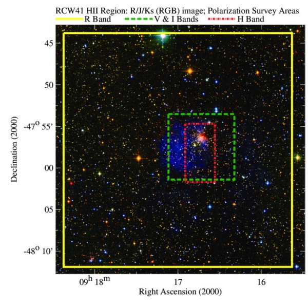
Figure 4.— The image above is a RGB combination of the R (DSS), J and Ks (2MASS) bands, showing both the H$\alpha$ extended emission related to the Hii Region (blue) and the position of the embedded stellar cluster. The areas mapped by the polarization survey are indicated by the boxes related to different spectral bands. The R optical band (yellow solid line) has been used to cover a large area ($28^{\prime}\times 28^{\prime}$) encompassing both the cluster and the Hii region, while V and I optical bands (green dashed box) cover a $8^{\prime}\times 8^{\prime}$ area more focused on the cluster. The NIR observations with the H band (red dashed-dotted box) cover a $3.5^{\prime}\times 7.0^{\prime}$ area towards the cluster and extended along the south.

From the difference in the measured flux for each beam, we derived the polarimetric parameters using a set of IRAF tasks specifically designed for this purpose (PCCDPACK package, Pereyra, 2000). This set includes a FORTRAN routine that reads the data files and calculates the normalized linear polarization from a least-square fit solution, which yields the degree of linear polarization ($P$), the polarization position angle ($\theta$, measured from north to east), and the Stokes parameters $Q$ and $U$, as well as the theoretical (i.e., the photon noise) and measured errors. The latter are obtained from the residuals of the observations at each wave plate position angle ($\psi_{i}$) with respect to the expected $\cos 4\psi_{i}$ curve. In further analysis of the polarimetric data, we adopted the greater value between both estimated errors.

Finally, in order to determine the reference direction of the polarizer, and to check for any possible intrinsic instrumental polarization, a set of polarimetric standard stars were observed at each night. The obtained polarizations degree for the observed unpolarized standard stars proved that the instrumental polarization are negligible for both telescopes and instrumentation.

In the case of the optical survey, V, R and I Johnson-Cousins’ filters (covering different areas over the studied region) were used. In Figure 4, it is shown a false-color image measuring about $30^{\prime}\times 30^{\prime}$ that corresponds to a combination of the R (DSS=blue), J(2MASS=green) and Ks (2MASS=red) images of the RCW41 region. The extended emission seen in blue is probably mostly due to the H$\alpha$ emission of the associated Hii region; the cluster objects are mainly seen in red and near the centre. The polarimetric R-band survey (yellow box - $28^{\prime}\times 28^{\prime}$) covers almost the whole area, while the V- and I-bands covers about $8^{\prime}\times 8^{\prime}$ of the region centered on the cluster (green dashed line). Each field was observed using exposures of 300 sec per half-wave plate position, and in order to cover the entire area of the R-band survey, a $3\times 3$ frames mosaic mapping was conducted at the CTIO’s 0.9 m telescope. The polarized standard stars for the optical survey were selected from the catalogs compiled by Tapia (1988) and Turnshek et al. (1990), corresponding to HD 298383, HD 111579, HD 126593 and HD 110984.

The NIR observations gathered at the 1.6 m telescope of the OPD observatory were performed using the H-band of the NIR camera CamIV, which has a $4^{\prime}\times 4^{\prime}$ field-of-view when mounted at this telescope. At each position of the half-wave plate, sixty 10 sec images were obtained (in order to avoid the detector’s non-linearity limit for the brighter sources), jittering the pointing by $12$ arcsec between each image in a cross-pattern, summing up to a 600 sec of total exposure time. Two fields were mapped in this manner, one centered on the cluster and a second one shifted towards de south, therefore covering a $3.5^{\prime}\times 7.0^{\prime}$ area as shown in Figure 4, by the red dashed-dotted box. The NIR polarimetric standards Elias 14, Elias 25 ($\rho$ Oph) and HD164740, were selected from Whittet et al. (1992), Wilking et al. (1980), and Wilking et al. (1982).

The complete polarimetric survey is presented in the Appendix (Table 3) with only a portion of the table given here just to demonstrate its format and content. The complete Table is given only in the electronic version of the article.

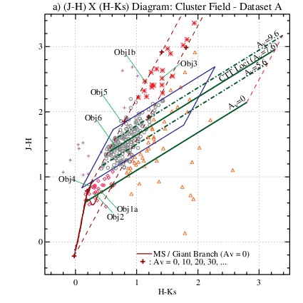
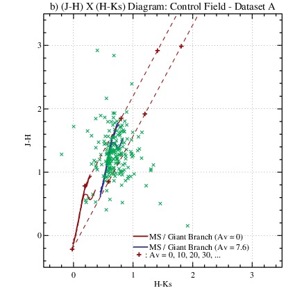
Figure 5.— Color-color diagrams for the cluster (a) and control (b) areas from Dataset A. Stars marked with Obj1-6 labels are objects previously studied through spectroscopic techniques (Roman-Lopes et al., 2009). The red dashed lines represent the reddening band from the standard reddening law, and the dark green lines denote the locus of CTT Stars. Different symbols and colors designate different sections from the diagram (a): the bulk of cluster’s stars is represented by gray open circles, with $1.1<J-H<2.2$, within the reddening band; also within the reddening band are stars presenting higher (red asterisks, $J-H>2.2$) and lower (pink diamonds, $J-H<1.1$) extinction values; purple plus signs and orange triangles respectively designate objects towards the left and right (therefore with color excess) of the reddening band. A small dispersion of $H-K\!s=0.1$ beyond the limits of the reddening band is allowed, to account for photometric uncertainties. All objects from the control area (b) are marked with green crosses.

3. Results and Analysis from the Deep NIR Photometry

3.1. Color-Color Diagrams

Valuable information regarding the nature of the cluster’s stellar population may be inferred from $(J-H)\times(H-K\!s)$ diagrams, which are shown in Figure 5. They were constructed from Dataset A, for objects in the cluster and control areas detected in all three bands. There are represented the unreddened main sequence (MS), along with the giant/supergiant branch locus (shown at the left bottom by the red solid line), as obtained from Koornneef (1983) and corrected to the 2MASS photometric system using the transformation proposed by Carpenter (2001). Also, the locus of the Classical T Tauri (CTT) stars (Meyer et al., 1997) is indicated in the cluster’s diagram by the solid dark green line, with the standard reddening law (Rieke & Lebofsky, 1985) being represented (in both cluster and control diagrams) by the red dashed lines. Different colors and symbols are used to represent objects from different parts of the diagram.

By comparing the distribution of sources in both diagrams, we can notice that despite the majority of control field stars show extinction levels similar to the cluster field stars, the objects from the cluster region present a much larger number of highly reddened objects and stars with color excess (respectively red asterisks and orange triangles). Furthermore, by analyzing the distribution of the majority of points from the cluster’s diagram (mainly the gray open circles), we note that they are approximately distributed along a strip (indicated by the solid blue line polygon) which is roughly parallel to the CTT locus (the dark green line). On the other hand, stars from the control field are more “vertically” distributed in the diagram, resembling the reddened Main Sequence locus. This may indicate that most of the stars from the cluster region are probably Pre-Main Sequence (PMS) stars.

3.2. Mean Visual Extinction

It is possible to take advantage of the fact that, the bulk of stellar objects from the cluster field lay in a distribution which is roughly parallel to the CTT line locus (blue polygon in Figure 5a), to estimate the mean visual extinction in the direction of the cluster. We initially will assume that the objects located inside the polygon area are CTT stars. Therefore, assuming the standard interstellar reddening law of Rieke & Lebofsky (1985), we have applied the de-reddening vector computing the visual extinction for each star inside the polygon. The average of these values yields a mean visual extinction of $A_{V}=7.6\pm 2.0$. We represent in Figure 5a the reddened CTT locus ($A_{V}=7.6$), as well as the uncertainty from this computation, i.e., the $A_{V}=9.6/5.6$ CTT loci (dark green dot-dashed lines). Although a large scattering of the CTT band is seen, we estimate that about $30\%$ of all stars from the cluster field are located within these limits. Besides, the interstellar extinction is probably spatially non-uniform along the cluster’s region and contamination from foreground objects is inevitable, which contributes to increase the observed scattering.

An independent computation of A_V may be inferred from spectroscopically confirmed O/B stars. According to the survey by Roman-Lopes et al. (2009), stars labeled as Obj1a, Obj2, and Obj4 in Figure 5a, probably belong to the group of cluster’s most massive objects (respectively B0v, O9v and B7v). Assuming that they have already reached the MS, we can obtain another value for the cluster’s mean visual extinction by de-reddening their observed (J-H) and (H-Ks) colors, using the intrinsic colors given by Koornneef (1983) and the interstellar extinction law taken from Rieke & Lebofsky (1985). Adopting this method, we have found the following A_V values, respectively for Obj1a, Obj2, and Obj4: $7.8\pm 1.4$, $7.0\pm 1.8$, and $6.4\pm 2.3$. All values are in the range 6-8 magnitudes, which is consistent with the computation obtained from the CTT candidates method.

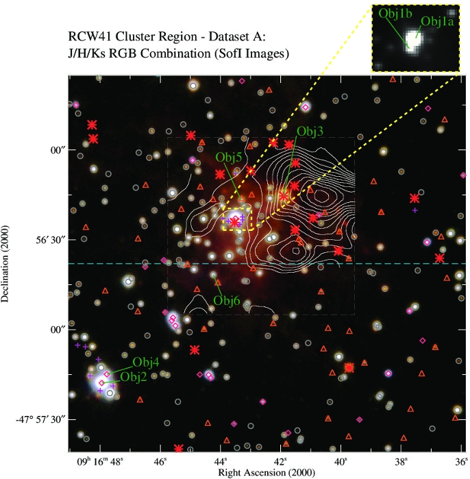
Figure 6.— Combined RGB image of the cluster region using J (blue), H (green) and Ks (red) images from SofI’s Dataset A. Contrast has been enhanced in order to reveal the bright extended emission surrounding the embedded stellar cluster. Stars are marked with colors and symbols related to their location on the color-color diagram (see Figure 5a), and objects indicated as Obj1-6 were previously studied through spectroscopic techniques (Roman-Lopes et al., 2009). The white-colored contours are from the HNCO survey by Zinchenko et al. (2000), representing the $10_{0,10}-9_{0,9}$ transition with the intensity levels starting from $15\%$ of the peak intensity ($1.5$ K$\cdot$ km s^-1), raising in steps of $7.5\%$.

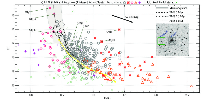
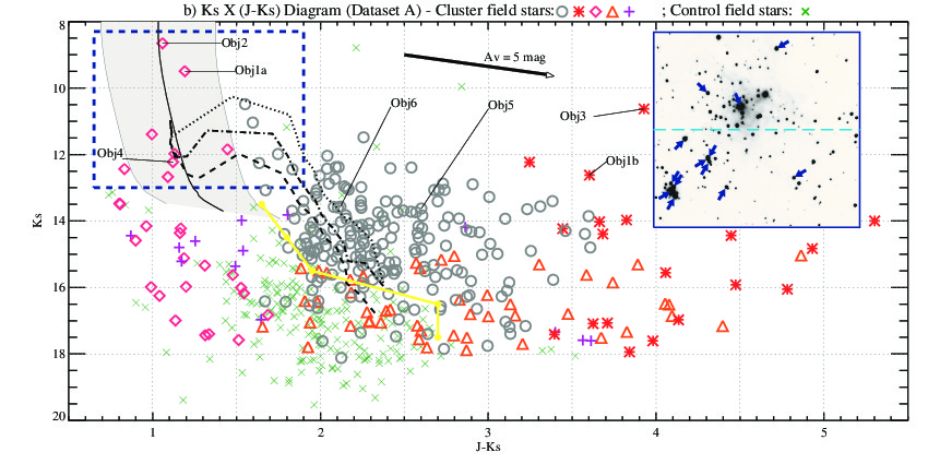
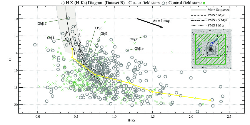
Figure 7.— Color-Magnitude diagrams using Dataset A (a: $H\times[H-K\!s]$; and b: $K\!s\times[J-K\!s]$) and Dataset B (c: $H\times[H-K\!s]$). The small 2MASS images inside diagrams a and c show the cluster and control areas used for each Dataset. Stars from the control areas are marked with green crosses, while cluster’s stars in diagrams a and b are marked with colors and symbols according to its location on the color-color diagram (Figure 5). All stars from the cluster area in diagram c are denoted by gray open circles. The MS and several PMS isochrones are indicated, and the yellow line provides a statistical separation between the contaminating field stars and objects from the cluster, as shown in Figure 8. In diagram b, the inset image shows the location of the cluster’s objects from the turn-on area (blue arrows), i.e., located within the blue dashed rectangle. Obj2 was saturated in Dataset B, and therefore is not shown in diagram c.

3.3. Spatial Distribution of the Cluster’s Stellar Population

Considering that the photometric properties of the cluster’s area indicate that it is composed by stellar populations with different characteristics (embedded PMS stars, foreground and background objects, stars with high extinction, etc), it is important to study their spatial distribution, relative to the cluster’s location. Figure 6 shows a false color image of the region obtained by combining the J/H/Ks images of Dataset A. Each detected star is marked with colors and symbols according to its location on the color-color diagram, as defined in Figure 5a, with the stars designed as Obj1-6 indicated by the green labels. Some very faint stars from the field were not marked because they were not detected in all three bands, and therefore were not assigned a location in the color-color diagram.

The cluster’s region is composed by two distinct structures: the main portion, which is associated to an extended emission visible mainly in the Ks band, is formed by a number of objects concentrated around the Obj1a/b stars (these two central objects present an angular separation of only 1.3 arcsec and are displayed in a close-up view at the top of Figure 6); the small sub-cluster region is located 1.1 arcmin towards the SE of the main cluster’s center, and hosts the Obj2, which is a O9v star (Roman-Lopes et al., 2009), presumably the most massive object in the field. According to Ortiz et al. (2007), Obj1a and Obj2 are the best candidates to ionization sources of the associated Hii region.

The contours shown in the map (colored in white) are from the HNCO survey of massive Galactic dense cores by Zinchenko et al. (2000), which covers mainly the central parts of the cluster. The HNCO molecule is most easily excited radiatively (rather then collisionally) inside the molecular clouds’ densest regions ($n>10^{6}\mathrm{cm}^{-3}$), being particularly sensitive to the far-infrared radiation field from warm dust, and therefore is a suitable tracer of regions at the vicinity of massive star-forming sites. As previously pointed out by Ortiz et al. (2007), the HNCO survey revealed an area supposedly swept out by stellar radiation around Obj1a/b, as well as the presence of a high-density region 30-50 arcsec NW of the central stars (Obj1a/b).

We may correlate this information with the location of stars with high extinction (marked with red asterisks). These highly obscured objects present $A_{V}$ values in the range 15 - 35, and are most commonly found toward the North of the field shown in Figure 6. From a total of 19 high extinction objects, 16 (i.e., 84% of them) are located above the cyan-colored dashed line which divides Figure 6 in Northern and Southern halves, suggesting an extinction rising gradient in the South-North direction. Furthermore, 9 of these stars (representing 47% of them) are located within the HNCO contours, indicating the expected correlation between the high density medium and the presence of highly obscured stars. Therefore, although background stars may be present, some of these are most probably highly embedded young cluster’s sources, and deserve special attention.

There is no clear trending for objects marked with gray open circles or orange triangles, being scattered along the entire area. However, for pink diamonds (i.e., lower extinction stars or also massive members of the cluster), there is a weak evidence that an anti-correlation exists relative to the positions of high extinction stars (red asterisks): 63% of the pink diamonds (17 among 27 stars) are located within the Southern area of the image. Although it is not possible to assert this unequivocally, this fact corroborates the idea that a rising extinction gradient occurs in the South-North direction. This evidence may support the idea that interstellar material surrounding Obj1a is only beginning to be swept out (according to the structure of HNCO contours), while the area around the subcluster (which hosts the O9v star) have already been cleaned due to the action of its strong winds.

3.4. Color-Magnitude Diagrams

In Figure 7 we show three color-magnitude diagrams for both the cluster and control areas. While the control field is probably composed by foreground and background main sequence and giant stars, the cluster’s field also contains members of the cluster itself. In order to locate the overlap region, stars from the control area (denoted by green crosses) were plotted in all diagrams. This is useful to identify stars from the cluster area presenting photometric characteristics of contaminating objects.

Figures 7a ($H\times[H-K\!s]$ diagram) and 7b ($K\!s\times[J-K\!s]$ diagram) were both created with colors and magnitudes from Dataset A, using the cluster and control areas as did in Section 3.1 (the inset in Figure 7a shows the cluster’s and control areas overploted in a small 2MASS Ks band image). Points from these two diagrams are plotted using the same color/symbol scheme as in Figure 5, therefore allowing us to identify the positions of the different groups previously defined in the color-color diagram. The zero age main-sequence (for solar metallicity) is represented by a 2MASS JHKs Padova isochrone (Bonatto et al., 2004), which is denoted by the black solid line surrounded by a gray band that accounts for the $\pm 2.0$ mag uncertainty in $A_{V}$. As a complement, we also plotted three pre-main-sequence (PMS) isochrones ($t=1$, $2.5$, and $5$ Myr, for solar metallicity) taken from young stellar evolution models by Siess et al. (2000). We used the cluster’s distance ($d=1.3\pm 0.2$ kpc) and the interstellar extinction as in Section 3.2. Furthermore, an arrow corresponding to an amount of 5 mag in visual extinction, was also included in each diagram.

Figure 7c is a $H\times(H-K\!s)$ diagram built with the H and Ks data from Dataset B, which provides a larger area around the cluster (see Figure 1). As shown by the inset, we have kept the same cluster’s area used in Dataset A (Figures 7a and b) and chosen a different control region, encompassing a wide area at the external borders of the region covered by Dataset B (defined by the green cross-hatched). This should allow a more complete probe of the field stellar population. Since J band data are not available from Dataset B, a position in the color-color diagram was not assigned, and therefore, we have simply used gray open circles to represent cluster’s stars and green crosses for objects from the control area.

By analyzing the distribution of the cluster’s and control’s stars in all three diagrams, we notice some striking common features. Initially, the majority of the point sources from the cluster’s region appear shifted from the MS locus, being displaced to its right with higher color values, i.e, over the region where the PMS isochrones are present. This indicates that the majority of the cluster’s sources are probably very young stars that still have not reached the hydrogen burning phase. However, as would be expected, some objects from the cluster area are located toward the left part of the diagram, occupying the same area as the control field stars, and therefore are probably members of the Galactic field stellar population. Also, from figures 7a and b, we can see that objects positioned toward the left side of the ZAMS are mainly those represented by pink diamonds and purple plus signs, i.e., lower extinction stars and objects with anomalous colors, therefore indicating that such objects are likely foreground stars. On the other hand, it is evident that some of the pink diamond brighter stars (for example, Objects 1a, 2 and 4), are in fact cluster’s members that have already reached the MS phase.

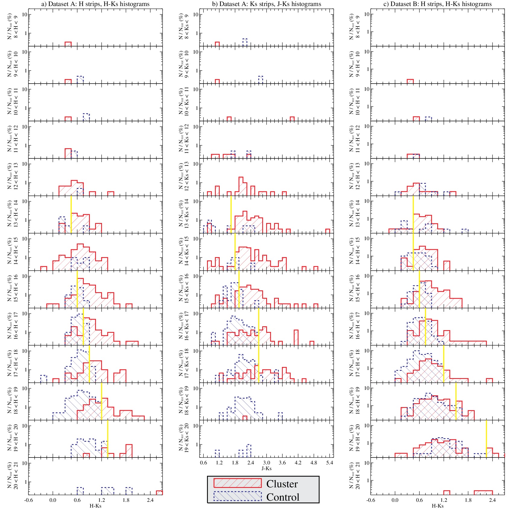
Figure 8.— Histograms of color indexes for cluster (red solid lines) and control areas (blue dashed lines), separated by successive strips of 1 magnitude wide. Histograms from parts a, b and c are directly related to the distribution of the stellar population in the color-magnitude diagrams respectively from Figures 7a , 7b, and 7c. Therefore, parts a and b are both from Dataset A, respectively representing histograms of $H-K\!s$ and $J-K\!s$ in magnitude divisions of $H$ and $K\!s$. Histograms from part c is from Dataset B, where the $H-K\!s$ color is used in bands of $H$ magnitudes. Each value in the histograms were normalized by the total number of stars used in each field. Vertical yellow lines are used in several histograms to help identifying contaminating stars from the cluster’s region, by separating the overlapping areas between control and cluster populations (at the left of the yellow line) from the population which is mainly composed by cluster’s stars (at the right).

Although the bulk of the cluster’s stars (represented by the circles), are located amongst the PMS isochrones, a certain number of objects appear distributed to the right in the diagrams, therefore presenting large $J-K\!s$ and $H-K\!s$ values. This is probably a combined effect of intrinsic infrared excess from PMS stars, non-uniform interstellar extinction along the clusters’ area, and photometric uncertainties. We specifically notice those stars represented by the orange triangles, which are well displaced toward the right showing high color indexes, which is an indication of emission from circunstellar disks. Furthermore, these objects are relatively faint with $H>16$, therefore probably corresponding to the very low-mass component of the YSO candidate sample.

Finally, the objects represented by red asterisks (identified as objects within the reddening band, but showing high extinction levels) appear presenting some of the highest $J-K\!s$ and $H-K\!s$ values. Although some of these stars may be background sources, considering the non-uniform and clumped nature of the interstellar environment around the cluster (see, for example, the HNCO emission contours in Figure 6 and the discussion in Section 3.3), it is possible that some of them are actually highly embedded cluster’s PMS stars. For example, it is highly probable that Obj1b (the close companion to the central star Obj1a, and that is marked with a red asterisk) is actually a massive YSO. More on this subject will be further discussed in Section 3.6.

3.5. The Cluster’s Evolutionary Status

The PMS isochrones from Siess et al. (2000) shown in Figure 7 may be correlated with the stellar distribution in the color-magnitude diagrams, to provide a mean estimate of the cluster’s age. However, contaminating field stars from the cluster’s area should be previously identified, at least in a statistical manner. Such identification is based on the overlap areas on the color-magnitude diagrams between the cluster and control populations.

In order to provide a more quantitative recognition of the contaminating objects, the following method have been adopted: the three color-magnitude diagrams from Figure 7 were divided in bands of 1 magnitude, and to every strip, a histogram was constructed, using the color index of each respective diagram. The results are shown in Figure 8, where histograms from parts a, b, and c are respectively related to the color-magnitude diagrams from Figures 7a, 7b, and 7c. Each histogram is divided between the cluster (red solid lines) and control (blue dashed lines) populations, and bins of 0.15 mag were used. The histograms were normalized by the total number of stars used in the color-magnitude diagrams of each area, namely: $N_{tot}$(Dataset A, cluster) $=302$, $N_{tot}$(Dataset A, control) $=202$, $N_{tot}$(Dataset B, cluster) $=384$ and $N_{tot}$(Dataset B, control) $=396$. Therefore, these diagrams represent the percentage fraction of stars within each magnitude strip and color bin.

A rough separation between the intrinsic cluster’s stars (mainly displaced toward the right of the histograms) and the field stellar population may be defined by the color index value where the cluster’s fractional number of stars becomes predominant relative to the control. To every histogram presenting a sufficient number of points, this value have been marked with a yellow vertical line. Therefore, it represents a separation criterion between the field stars (objects from the left of the yellow line) and the intrinsic cluster’s population (stars from the right of the yellow line). These values were also indicated in Figure 7 by the yellow connected dots and lines. This provides an appropriate scheme to roughly de-contaminate the color magnitude diagrams, therefore allowing a more clear analysis of the isochrones’ positions relative to the distribution of possible intrinsic points from the cluster.

Specially when analysing Figures 7a and 7c (the $H\times[H-K\!s]$ diagrams), we notice that the yellow separation lines passes exactly between the locus related to $t=2.5$ Myr and $t=5.0$ Myr. Moreover, in these two diagrams, the bulk of the cluster’s points (gray open circles), which are toward the right of the yellow line, seems to roughly define a band around the $t=2.5$ Myr isochrone.

On the other hand, the turn-on point is better defined in the $K\!s\times(J-K\!s)$ diagram (Figure 7b), as indicated by the blue dashed rectangle, which encompassed both objects that have already reached the MS, and those that are currently leaving the PMS stage. Notice that over the MS region, below the turn-on point for the $t=5.0$ Myr isochrone, there is a small gap for cluster’s sources with magnitudes in the range from $K\!s=13$ up to $K\!s\approx 14$ (from whereon contaminating objects seem to dominate), suggesting that there are no stars from the cluster with $t>5.0$ Myr. Furthermore, the Obj4 star, whose distance is consistent with being an intrinsic cluster’s source (Roman-Lopes et al., 2009), is located over the MS, at the midway between the $t=2.5$ and $t=5.0$ Myr isochrones.

These evidence suggest that the cluster’s mean age is between $2.5$ and $5.0$ Myr. Moreover, these analysis reveal that a sequential star formation scenario may have occurred within this region. The spatial location of objects from the turn-on area in Figure 7b (within the blue dashed rectangle) is indicated by blue arrows at the inset image in the same diagram. It is evident that most of these objects (10 among a total of 13) are positioned closer to (or within) the subcluster, instead on the central main cluster area (as would be expected if mass segregation processes had already taken place). Therefore, a plausible explanation to this evidence may be that the most massive objects (located at the subcluster), were formed earlier, subsequently inducing star formation at the main cluster area.

This evolutionary view is supported by the fact that the interstellar material near the subcluster seems to have already been swept out, while at the cluster area denser clumps are still present (see Section 3.3). If the multi-epoch formation hypothesis is in fact true, the large spread of cluster’s points on the color-magnitude diagrams towards higher color values could also be explained by an intrinsic age spread of the studied stellar population.

3.6. Analysis of Individual Objects with known Spectroscopic Properties

The spectroscopic features of several specific objects previously studied by Roman-Lopes et al. (2009), may now be correlated with the objects’ position on the color-color and color-magnitude diagrams. The same stars from that survey were renamed as Obj1-6 and are indicated in Figures 5, 6, and 7.

Three of the most massive objects from the cluster – Obj1a, 2, and 4 – were respectively classified as B0v, O9v, and B7v-B8v stars. Their location on the color-magnitude diagrams (Figure 7) are consistent with stars that have already reached the MS.

Obj1b shows spectral lines characteristic of YSO’s, and according to Ortiz et al. (2007), the set Obj1a+b also indicates features of warm dust, such as infrared emission beyond $5\mu$m (probably coming from Obj1b). In fact, this object is located within the high-extinction region of the color-color diagram, an indication of its embedded nature. Furthermore, we notice that its K-band spectrum (see Figure 6 from Roman-Lopes et al. (2009)) presents features which are very similar to the spectrum of T Tau Sb, the third member from the T Tau system (Duchêne et al., 2002): both sources show a large Br$\gamma$ emission (which is a strong accretion signature), as well as several absorption CO overtones. This evidence suggests that Obj1b, the close companion to the massive B0v central object (Obj1a), is a very young T Tauri star. The presence of this young object near the center of the main cluster region provides additional support to the idea that star formation within this area have been triggered by the earlier star formation activity at the subcluster, as discussed in Section 3.5.

Although the sources labeled as Obj5 and Obj6 were previously classified as late-type field stars, their position on the color-magnitude diagrams (Figures 7a, b, and c) are consistent with a classification as T Tauri stars. Even though their spectroscopic features may be interpreted as from typical low mass late-type stars, observations have been reported of Class I stars with few spectroscopic signs of youth. Two examples are the IRAS 03220+3035(S) and IRAS F03258+3105 sources, from the NIR spectroscopic survey by Connelley & Greene (2010), which were classified as young YSO’s, despite presenting K-band spectra only with some CO overtones in absorption and almost no Br$\gamma$ emission, hence being very similar to Obj5 and Obj6. Therefore, if we also take into account their position at the very crowded area near the cluster’s center (see Figure 6), these sources are most likely T Tauri stars, members of the cluster.

Other interesting properties are related to Obj3, that is a highly reddened source, and has NIR colors corresponding to a visual extinction of $A_{V}>20$, which is consistent with its spatial location among the HNCO contours (Figure 6). Although the previous analysis of its K-band spectrum showed that it could be a typical late-type background star, its position in the color-magnitude diagram suggests that it may also be interpreted as a highly reddened medium mass YSO. A careful analysis of its spectrum show a weak set of CO absorption lines, which is usually a feature of low-mass YSO’s. However, its high NIR luminosity rather suggests a more massive nature. Therefore, a valid explanation for the weakness of these lines could be due to veiling of the photosphere and CO bands by the circunstellar dust emission, as suggested by Casali & Eiroa (1995). In this case, an anti-correlation of these lines’ intensity with the NIR color excess is expected. Although more observations are necessary to fully characterize this source, these evidence indicate that Obj3 is likely a medium mass YSO from the cluster.

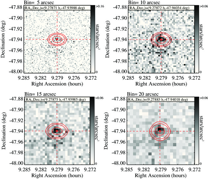
Figure 9.— Stellar density distributions to different bin sizes, created using the photometric positions of Dataset B. The gray-scale is related to the stellar density, where darker tones represent a higher density, as can be inferred by the scale bars. Bi-dimensional Gaussian fits applied to each distribution are represented the red contour lines, which are related to the following levels: $0.013$, $0.015$, and $0.030$ stars/arcsec². The center positions computed from the Gaussian fits are specified at the top of each diagram, and are indicated as a red bullet.

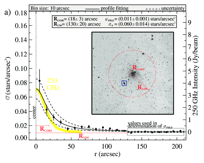
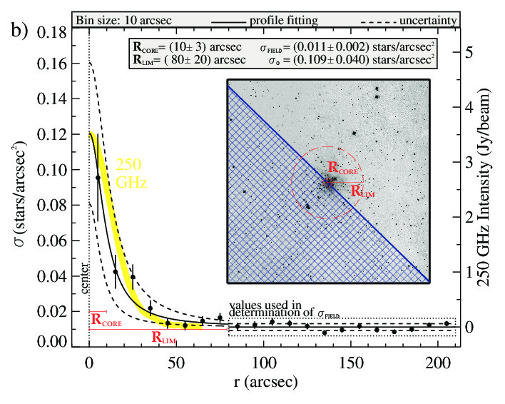
Figure 10.— (a) King profile fitting using concentric rings around the cluster’s center position. The values obtained for $\sigma_{0}$, $R_{core}$, $\sigma_{field}$, and $R_{lim}$ are expressed at the top of the diagram, and the spatial size of $R_{core}$ and $R_{lim}$ are indicated as dashed red circles in the Ks image from Dataset B (inset). The error bars represent the Poisson uncertainties. The $\sigma_{field}$ parameter, which represents the uniform stellar density from the field, is separately computed, by taking the mean value (and the standard deviation) of points with $r>R_{lim}$. (b) The same King profile fitting, ignoring the blue cross-hatched area, which contaminates the RDP due to a stellar density scattering toward the South-East. Notice the sharper format of the curve fitting in this case. In both diagrams (a) and (b), the thick yellow line represent the radial density profile of the 1.2 mm dust continuum emission (250 GHz) originated from the cluster’s direction, defining an almost spherical projected core, as described by Pirogov et al. (2007) and Pirogov (2009). The scale at the right represent the 250 GHz intensity, and the peak of this radial density profile is adjusted to match the peak of the stellar density from the King function, for comparison purposes.

3.7. Cluster’s Center Determination and Radial Density Profile

In order to perform a rigorous analysis of the cluster’s Radial Density Profile (RDP), it is important to determine its mean center. Therefore, we have used the Ks image from Dataset B, divided the region into bins of specific widths ($5$, $10$, $15$, and $20$ arcsec), and computed the stellar density distribution. The result is shown in Figure 9, where the gray-scale represents the number of stars per bin area.

The cluster’s center position for each bin width was determined through bi-dimensional Gaussian fits to the stellar density distributions, represented by the red contour maps superposed to each diagram in Figure 9. A mean value has been computed, resulting in ($\alpha_{\mathrm{c}}$,$\delta_{\mathrm{c}}$)=($9^{\mathrm{h}}16^{\mathrm{m}}43.5^{\mathrm{s}}$,$-47^{\circ}56^{\prime}24.2^{\prime\prime}$), with an uncertainty of ($0.2^{\mathrm{s}}$,$0.9^{\prime\prime}$). Although the cluster’s stars appear slightly scattered toward the South and South-East (near the subcluster), a highly peaked concentration appears around $\alpha_{\mathrm{c}}$,$\delta_{\mathrm{c}}$, the cluster’s center.

The morphology of the RCW41 cluster’s RDP may be studied by fittings of a two-parameter King function (King, 1962, 1966), which may be approximately described in terms of the central density ($\sigma_{0}$) and the core radius ($R_{core}$). This was achieved by positioning several circumcentric rings around the computed center, with widths of $10$ arcsec each, and computing the stellar density as a function of the distance from the center ($\sigma(r)$). The obtained density profile was fitted by the following equation:

$$\sigma(r)=\sigma_{field}+\frac{\sigma_{0}}{1+(r/R_{core})^{2}}$$ (1)

The results are expressed in Figure 10a, where the points indicate the stellar densities at each ring, and the King function fitting is denoted by the solid line, together with the uncertainty curves (dashed lines) obtained from the uncertainties of the fitted parameters. Starting from the center, the stellar density decreases towards larger radius, and the point where the cluster’s density completely merges with the field density is visually identified as $R_{lim}$, i.e., an approximate value for the cluster’s limiting radius.

Note that a bump extending from $r\approx 65$ to $110$” appears in this radial profile, which is due to the stellar scattering towards the south-east area (which includes the sub-cluster – small blue box in Figure 10a). In Figure 10b, we have removed this area from the RDP analysis (blue cross-hatched region), in order to provide a cleaner fitting only of the cluster’s main concentration, i.e., the stellar densities were computed from increasing half-rings at the Northwest area of the field. The new King function is much sharply concentrated toward the center in this case, showing a large decrease of $44\%$ in $R_{core}$ and $38\%$ in $R_{lim}$. The estimated value of $R_{lim}$ indicates that the control areas used in the photometric analysis from the previous Sections, are sufficiently distant from the cluster’s main structure, therefore avoiding significant contamination.

Lada & Lada (2003) pointed out that embedded stellar clusters may be morphologically classified as hierarchical-type (with multiple peaks at the density profile, frequently found scattered over a large spatial scale) or centrally condensed-type (highly concentrated distributions, with relatively smooth RDPs). Although the density distributions show that the cluster do present some isolated stellar concentrations, the relatively smooth fit of the King function indicates that it is probably of the centrally condensed-type. This structural type is a common feature of very young stellar clusters, since most of the stars have not yet dispersed throughout the field, and are still heavily concentrated around the center.

Such morphology may be correlated with 250GHz observations of the 1.2mm dust continuum emission towards this region (Pirogov et al., 2007), that defines an almost spherical core in which the cluster is probably immersed in. Based on these observations, Pirogov (2009) computed a power law radial density profile of the dust emission, which is shown in Figures 10a and 10b by the thick yellow line (the peak emission was adjusted to match the maximum value of the King function). One may note that both distributions (from the dust emission and from the stellar density) are similar in size, suggesting that the stellar system is still embedded within part of the original cloud in which star formation was initially ignited. Therefore, the presence of such dense interstellar material increases the gravitational potential and so the physical bounding of the system, aiding to keep the stars spatially concentrated. The centrally condensed-type stellar cluster occurs because of the interstellar gas and dust from the parental molecular cloud, which are still present in the cluster’s region, and probably beginning to be swept away due to the action of the new-born massive stars.

It is important to point out that in the above mentioned comparison, the centers of both the dust emission radial profile and the King function, are not exactly the same, being separated by about $\sim 11$ arcsec. Furthermore, Pirogov (2009) adopted a much larger distance to this object (2.6 kpc), as compared to the value of 1.3 kpc spectroscopically determined by Roman-Lopes et al. (2009). However, the difference is irrelevant in this case, since we have converted the spatial dimensions to angular sizes in Figure 10.

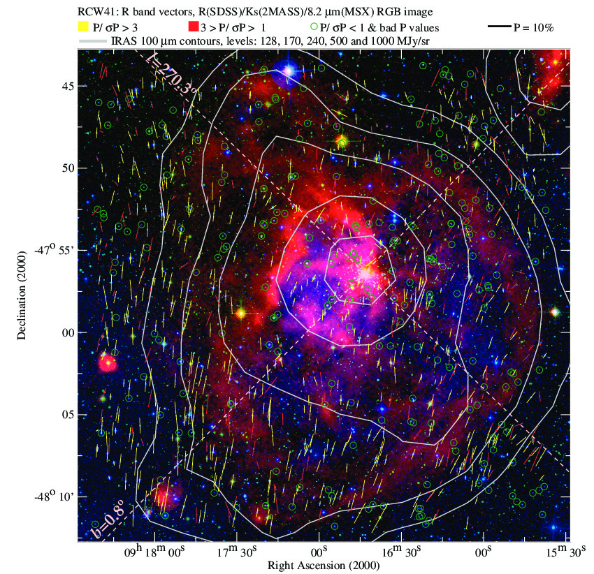
Figure 11.— Distribution of R-band polarization vectors at the RCW41 region. The image is a $30\times 30$ arcmin RGB combination of the DSS R-band (blue), the 2MASS Ks band (green) and MSX 8.2$\mu$m emission (red). Notice the large mid-IR ring or bubble (red) surrounding the blue-colored ionized area. The embedded cluster is located nearly at the center of the region. Vectors’ sizes are proportional do the polarization degrees and colors are related the data quality, as specified above the diagram. Green circles denote objects with poor ($P/\sigma_{P}<1$) or bad polarization values. Gray lines are the IRAS 100$\mu$m contours, showing the 128, 170, 240, 500, and 1000 MJy/sr emission levels.

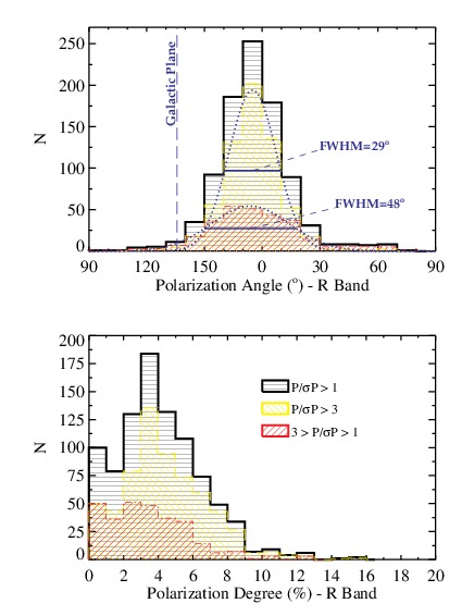
Figure 12.— Histograms related to the R-band polarimetric dataset, representing the polarization angle (top) and polarization degree (bottom) distributions. Yellow and red colors respectively denote the poor and good-quality data, while the black histograms consider the entire sample presenting $P/\sigma_{P}>1$.

Figure 13.— (a) $(J-H)\times(H-K\!s)$ color-color diagram using 2MASS data for the R-band polarimetric sample; (b) $P_{R}$(%) $\times(J-H)$ diagram constructed from a correlation between the R-band polarization data and the 2MASS magnitudes; (c) Spatial distribution of probable foreground (green crosses) and background or embedded stars (orange vectors, represented as asterisks in diagrams (a) and (b)).

4. Results and Analysis from the Optical/Near-Infrared Polarimetry

4.1. The Large-scale Distribution of R-band Polarization Vectors

The R-band polarization survey covers a large area around the RCW41 region, encompassing both the stellar cluster and the ionized area, as previously shown in Figure 4. A polarization degree and angle were assigned to every point-like source detected in the field, and by this manner we have constructed a map of the Hii region showing the distribution of polarization vectors superposed to each star, as exposed in Figure 11. The vectors’ orientations indicate the predominant direction of the electric field oscillations related to the stellar light beam, and assuming the standard grain alignment mechanisms, the vectors trace the sky-projected component of the interstellar magnetic field lines (Davis & Greenstein, 1951).

In this image, the size of each vector is proportional to the polarization degree (a $10$% sized vector is indicated at the top-right of the graph as reference), and the vector’s colors are related to the quality of the polarization measurement: good quality measurements, with $P/\sigma_{P}>3$, are shown in yellow, while lower quality data, with $3>P/\sigma_{P}>1$, are shown in red. Green circles denote objects with $P/\sigma_{P}<1$ or stars with bad polarization values (i.e., affected by cosmic rays, bad pixels of the detector or light beam superposition with close companions). Therefore, all optically detected objects from this survey are marked, either with a vector or a green circle, according to the above mentioned criteria.

Since the observations were done by integrating the light of all stars from the field with the same exposure time, the classification of an individual measurement among one of these groups depends on the stellar brightness (which increases the individual signal-to-noise ratio) and also on the intrinsic polarization degree from the source (therefore, unpolarized sources naturally have larger probability to fall on the $P/\sigma_{P}<1$ classification).

Considering that many stars are too obscured to be detected by the optical survey, only the brightest sources were visible. Even though, these observations are still useful to study the large-scale properties of the magnetic field structure around the Hii region, as will be shown in the following sections. However, it is important to point out that, considering the $1.3$ kpc distance to the cluster, a fraction of these stars are foreground objects, and therefore their observed polarization levels are possibly mainly caused by interstellar components not related to the RCW41 region. These properties will be further analyzed in Section 4.2.

The background image used to produce Figure 11 shows interstellar structures related to the star-forming region extending into a large area around the embedded stellar cluster. The image is a RGB combination of: the DSS R-band image (blue), showing optically visible stars and the ionized region (the H$\alpha$ emission is within the spectral region defined by the R band); the 2MASS Ks image (green), indicating the location of several obscured stars visible only in the near-infrared, including the associated stellar cluster, nearly at the image’s center; the MSX 8.2$\mu$m mid-infrared emission (red), showing mainly the radiation from the warm dust and polycyclic aromatic hydrocarbons (PAHs).

A striking feature seen in this image is that the mid-infrared emission (red) defines a great ring or bubble of warm dust and PAHs that encompasses the ionized area denoted by the extended emission in blue. This structure suggests that UV radiation from massive stars and high energy photo-ionized electrons from inside the Hii region heats the dust grains and excites the PAHs from the surrounding environment, generating the “envelope” type of emission. It is not uncommon to find mid-infrared emission of PAHs at the outer edges of Hii regions, as revealed for example by the Spitzer GLIMPSE survey of the Galactic Plane (Churchwell et al., 2006, 2007).

Some mixture between the R-band and mid-infrared emission is seen in the direction of the cluster, where several interstellar filaments extend almost radially from it. Such morphological structure will be further analyzed in Section 4.5.

Another interesting information is provided by the IRAS 100$\mu$m emission which is attributed to the colder dust component and is represented in Figure 11 by the gray contours. Note that the 100$\mu$m emission shows a peak almost centered on the cluster’s area and that the outer contours (especially the $170$ MJy/sr isophote) roughly follow the morphology of the hot dust ring from the mid-infrared radiation, suggesting the existence of a cold dust “cocoon” around the entire area.

Comparing the global distribution of polarization vectors with the direction of the Galactic Plane (the $b=0.8^{\circ}$ line), we note that both directions are not correlated. All-sky optical polarization surveys have shown that, particularly along the Galactic Plane, polarization vectors tend to present an overall horizontal orientation, i.e., parallel to the plane (Mathewson & Ford, 1970; Axon & Ellis, 1976; Heiles & Crutcher, 2005). However, as noted by the latter authors, the polarization vectors lose this tendency on the magnetic “poles”, located at $l\approx(80^{\circ},260^{\circ})$. The VMR is located along one of such “pole” (the RCW41 cluster is at $l=270.3^{\circ}$), and therefore the correlation between polarization vectors and the Galactic Plane direction is indeed not expected.

The distribution of polarization vectors presents some characteristics that can be related with the features of the Hii emission region. Note that toward the ionized area, and specially near the cluster, the vectors’ sizes are small when compared to the outer vectors. This evidence indicates a decrease of polarization degree values toward the center of the region. Furthermore, at the right side of the field, a global bending of the vectors’ directions is seen both at the area’s bottom-right and top-right portions, resembling to roughly follow the curvature of the IRAS 100$\mu$m emission contours in these regions. Such properties will be further analyzed in Section 4.3.

It is important do point out that, since a fraction of the sample is composed by YSO’s with infrared excess, some of these sources may contribute with a contaminating polarized emission from the circunstellar disk. However, the large-scale correlated pattern of polarization angles seen in the map may not be explained by intrinsic polarization. The overall characteristics are best described by interstellar polarization due to dust dichroic absorption, with some possible scatter in polarization angles due to individual disk emission from some sources.

Figure 12 shows histograms of polarization angle and polarization degree divided by different $P/\sigma_{P}$ intervals. The Gaussian fits to the angle histograms show that the dispersion (indicated by the FWHM lines) of the $3>P/\sigma_{P}>1$ data (red) is larger than the $P/\sigma_{P}>3$ case (yellow), an expected trend given the lower data quality. However, both distributions are quite well correlated, showing polarization angles predominantly in the $160^{\circ}-10^{\circ}$ range. Moreover, by comparing the orientations of higher and lower quality vectors in Figure 11, it may be noted that these are quite well correlated locally, indicating that the lower quality data may also be included in the analysis. Polarization degrees varies between $0$ and $\sim 16\%$, with a large number of stars peaking at $P_{R}\approx 2-6\%$.

4.2. Correlation with 2MASS photometry

Since the individual stellar distances for the polarimetric survey are not available, we shall take advantage of the 2MASS data to approximately infer the foreground, background and intrinsic cluster’s populations. Given that the Hii region is located at $1.3$ kpc from the sun, it is important to evaluate if the interstellar polarization of objects from such distance range are significantly affected by the nearby structures along the same line-of-sight. Therefore, the goal is to identify, at least statistically, foreground objects and analyze their polarization levels in comparison with the typical values from the field.

Figures 13a and b show respectively the $(J-H)\times(H-K\!s)$ color-color and the $P_{R}\times(J-H)$ diagrams using the R-band polarimetric sample and the associated 2MASS data. Figure 13a shows that the bulk of polarimetric points present $(J-H)$ values in the range $0.5-1.1$ mag, in contrast with the previous photometric analysis (Figure 5), where it has been shown that stars both from the cluster and control regions are somewhat more reddened. This is probably due to a combination of two factors: (1) the earlier analysis was carried out toward a much smaller area, concentrated on the cluster, where the $A_{V}$ values are statistically higher; and (2) the polarimetric survey is optically limited, and therefore only the brightest sources were detected.

Figure 13b shows that, for those objects having $J-H\gtrsim 0.9$, there is almost no star presenting $P_{R}<1\%$. This effect is emphasized by the vertical ($J-H=0.9$) and horizontal ($P_{R}=1\%$) green dashed lines in this diagram. This is a suggestion that objects obscured by the molecular cloud (and therefore located behind or within it) show a minimum polarization level equal to $1\%$. As a consequence, stars presenting polarization values below this limit are probably foreground objects. Such points are marked with green crosses, and define a thick band around the unreddened MS locus in the color-color diagram (Figure 13a), a further evidence that they are mainly foreground, not absorbed stars. Moreover, their spatial location on the field is uniform (Figure 13c), as expected for a randomly distributed group of foreground objects along the line-of-sight.

We conclude that although a small polarization level due to foreground structures is probably included in the stellar light for most of the objects in the observed field, this level is small when compared to the typical polarization levels found for the region (which is mainly between $2$ and $6\%$, as suggested by the polarization distribution given in Figure 12). In fact, Santos et al. (2011) have shown that in the directions near $l\sim 260^{\circ}$ over the galactic plane, polarization degrees in the V band are smaller than $1\%$ at least up to a distance of $400$ pc from the sun. Therefore, it is expected that a major fraction of the polarization vectors for the observed field indeed map the magnetic field lines within the Hii region.

By analyzing Figure 13a, we note that a group of points (marked with orange asterisks) are located above a small gap (at $J-H\approx 1.1$) within the reddening band of the color-color distribution. The $A_{V}=7.6$ MS reddened locus (as calculated for the cluster, Section 3.2) is superposed to these points, showing that these stars are reddened by the molecular cloud, and therefore are probably either background or embedded objects. Their spatial distribution is also shown in Figure 13c. Open circles, which comprises the main group of stars from the field, have typical polarization degrees above the $1\%$ level for foreground objects and typical $J-H$ values below the $1.1$ estimated limit for background and embedded stars. Therefore, this group is probably composed by a mixture of foreground, background, and mainly embedded objects in the Hii region.

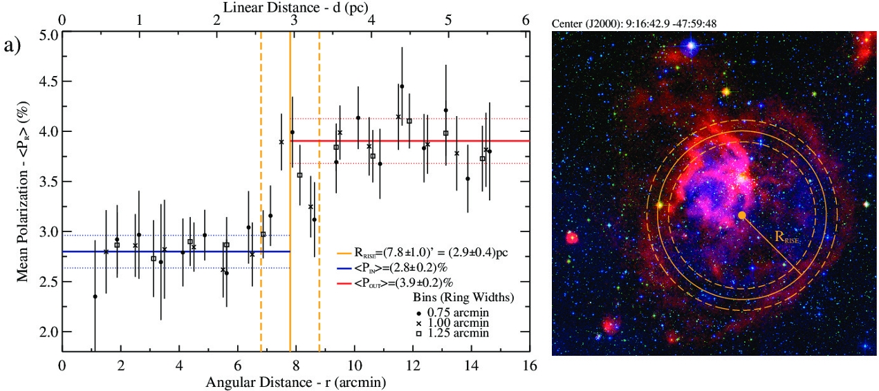
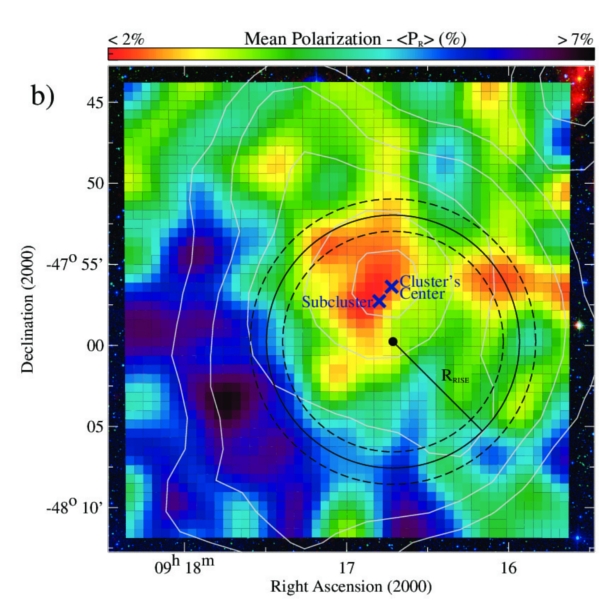
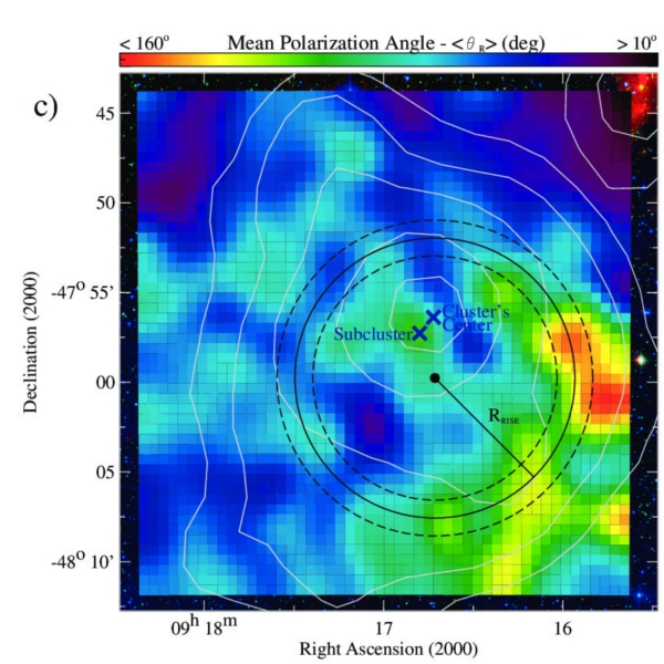
Figure 14.— (a) Analysis of the radial dependence of mean polarization degree inside the RCW41 ionized area, where the center has been chosen based on the R-band extended emission (as shown by the blue color at the image toward the right). An abrupt rise in polarization degree is found roughly coinciding with the position of the warm dust/PAHs ring seen at the MSX 8.2$\mu$m mid-infrared emission (red). (b) Mean polarization map, built by averaging the polarization values of point-like sources into an image of $50\times 50$ equal divisions. Notice that mean polarization nearby the cluster are smaller than the typical values from the field, and a large area at the bottom left following the ridge of the Hii region shows an increase of polarization values. (c) Mean polarization angle image, following the same procedure used in part (b). A global bending of the sky-projected magnetic field lines is found at the bottom right of the image, also following the rim of the ionized area.

4.3. Large-scale Mean Polarization Degree and Angle Maps

In order to analyze further the evidence that the degree of polarization is lower inside the Hii region, we have chosen an approximate center of the ionized area (based on the R-band extended emission, represented by the blue color in the image shown in Figure 11), and studied the behavior of the mean polarization as a function of this radial distance from the center. This analysis is displayed in Figure 14a: beginning from the selected center position ($(\alpha,\delta)_{J\!2000}$ = (9 16 42.9, -47 59 48)), several circumcentric rings of increasing radius were built, and inside each ring, the Q and U Stokes parameters from individual objects (with $P/\sigma_{P}>1$) were averaged, therefore allowing to compute the mean polarization value associated to that ring and its associated standard deviation. Three different ring widths were used in this analysis ($0.75$, $1.00$ and $1.25$ arcmin), and the results are identified with distinct symbols in Figure 14a. Therefore, each mean polarization value was plotted as a function of the angular distance from the chosen center.

A sharp increase in mean polarization degree (from $\approx 2.8\%$ to $\approx 3.9\%$) was found at a distance of $\sim 7.8$ arcmin from the center of the Hii region (corresponding to $\sim 2.9$pc, assuming that the cluster is located at $1.3$kpc from the sun). Such distance is denoted by an orange circle in the RCW41 image of Figure 14a. By comparing the position where the polarization degree increases (with respect to values inside the Hii region) with the MSX 8.2$\mu$m mid-infrared emission (red), we find a striking evidence that such position roughly corresponds to the warm dust and PAHs “bubble” that encloses the ionized gas.

Given these evidences, we have attempted to build a “mean polarization image” of the RCW41 region, based on the R-band survey. To achieve this result, we have divided the spatial region where the polarimetric data is distributed into $50\times 50$ intervals of equal width. Considering each observation inside a specific division, a mean polarization value was computed (only objects having $P/\sigma_{P}>1$ were used). In order to account for cases where no stars were available inside a particular division, a smoothing routine was applied, returning the same image, but averaged locally by using a small box that runs through the entire array. The result is shown in Figure 14b, where the polarization image is superposed on the actual picture of the RCW41 Hii region. Redder colors correspond to lower polarization levels while bluer colors indicate higher polarization levels, as specified by the colorbar given at the top of the diagram. The location of the cluster (and the associated sub-cluster), as well as of the ring where mean polarization is found to sharply increase, are also indicated.

Note that nearby the cluster (and slightly toward the northeast of it), we find an area where polarization mean values are lower, in comparison with typical values for the field, presenting $P\lesssim 2\%$ (marked in red). Furthermore, toward the left and bottom side of the area (southeast), we find a large region where the polarization degree is higher ($P\sim 6\%$, marked in dark blue). This region marks the transition border between the inner and outer sides of the southeast part of the Hii region, and is probably responsible for the sharp increase in polarization detected in Figure 14a.

Two models may be proposed to explain the decrease of polarization toward the ionized region: (1) given that temperature values of the local interstellar medium and the radiation field from hot stars are probably higher inside the Hii region, it is expected that mechanisms of grain alignment are disturbed by the turbulent medium, hindering the alignment efficiency and therefore providing lower $P$ values. Polarization efficiency may also be affected if the intensity of the magnetic field inside the photo-ionized area is intrinsically weaker, which may be true if field lines have been pushed aside by the expansion of the Hii region; (2) dust grains have been swept away from inside the Hii region, due to the action of intense stellar winds from the newborn stars, therefore resulting in a lower dust column density and consequently lower $P$ levels. Obviously, if the second model is true, a similar decrease of interstellar extinction as a function of the distance from the center would be expected. Further discussion on the distinction between both models will be carried out in Section 5.

We have also constructed a “mean polarization angle image”, using the same procedures described above. The result is shown in Figure 14c, where yellow and red colors represent vectors slanted to the right and blue colors are regions with mean polarization angles slanted to the left (with respect to the vertical orientation). By this diagram, we are able to highlight global changes in polarization angle with respect to the typical values found in the field. In fact, we note that toward the bottom right of the image (southwest) , a large area marked with green/yellow/red colors indicate a global slanting of the polarization vectors toward the right. Furthermore, such regions seems to roughly follow the outer contour of the ionized area, indicated by the circle of Figure 14a. Such inclination of the polarization vectors may also be seen in Figure 11, as pointed out earlier in Section 4.1.

This structure suggests that the physical processes that generated the Hii region, followed by the expansion of the ionized area, caused a global deflection of the original magnetic field lines in the field. Such deflection of the magnetic field lines around the expanding ionization front is most prominent toward the southwest area surrounding the Hii region, as exposed in Figure 14c. As an example, Matthews et al. (2002) describes another region were a similar distortion of magnetic field lines was observed toward NGC 2024, with polarization vectors being swept due to the expansion of the associated Hii region. Tang et al. (2009) also described a similar effect toward G5.89, a $\sim 0.01$ pc sized ultra-compact Hii region at a much earlier evolutionary stage ($\sim 600$ years), already displaying significant distortion of the magnetic field lines as a consequence of the expansion of a shell-like structure.

4.4. Wavelength Dependence of Polarization and Determination of the Total-to-Selective Extinction Ratio

It is possible to take advantage of the polarimetric survey in multiple spectral bands to analyze specific properties of the dust particles along this region. For instance, the grain size distribution causes a direct influence on the underlying interstellar law, which is generally assumed to follow a standard behavior. Therefore such analysis will enable us to directly test this hypothesis, at least in the direction of the cluster and nearby surroundings, were V, R, I and H polarization data overlap (see Figure 4).

It is well known that an empirical law, known as the Serkowski relation, may be used to describe the spectral dependence of the interstellar polarization (Serkowski et al., 1975):

$$P_{\lambda}=P_{max}\exp{\left[-K\ln^{2}{\left(\frac{\lambda_{max}}{\lambda}\right)}\right]}$$ (2)

where the typical value of the parameter $K$ is $1.15$, and $P_{max}$ and $\lambda_{max}$ denote respectively the maximum polarization value and the wavelength where such maximum point is reached. Furthermore, it is also known that when stellar light trespasses different dust layers with different grain alignment conditions, it is possible that the resulting beam will present a spectral dependence of the polarization angle, usually represented as a rotation of $\theta$ with respect to $\lambda^{-1}$ (Gehrels & Silvester, 1965; Coyne, 1974; Messinger et al., 1997).

By analyzing the overlap region between the polarimetric surveys in the V, R, I and H bands, we have selected stars with VRIH or at least VRI observations, where the requirement $P/\sigma_{P}>3$ was fulfilled in all observed bands. Our polarimetric sample contains 34 objects meeting these conditions. Values of $P_{max}$, $\lambda_{max}$, and a measurement of the rotation of the polarization angle were obtained for each of these stars. As an example, Figure 15a illustrates the results obtained for one of them, i.e., the $P\times\lambda^{-1}$ graph (along with the adjusted Serkowski curve) and the $\theta\times\lambda^{-1}$ diagram, also showing the fitted values for this particular case.

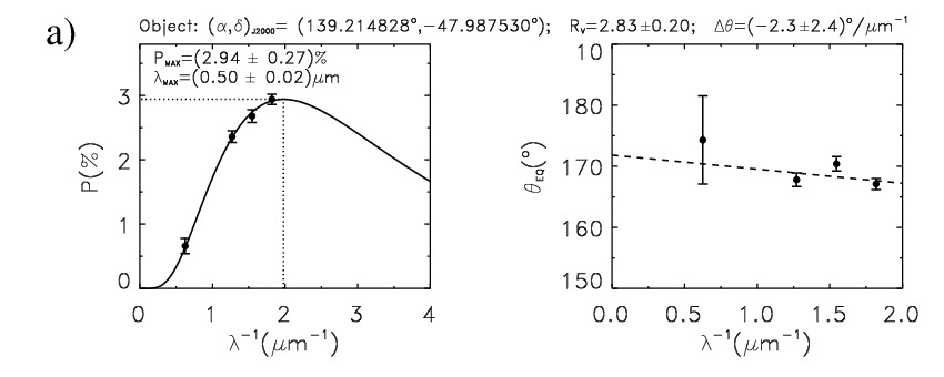
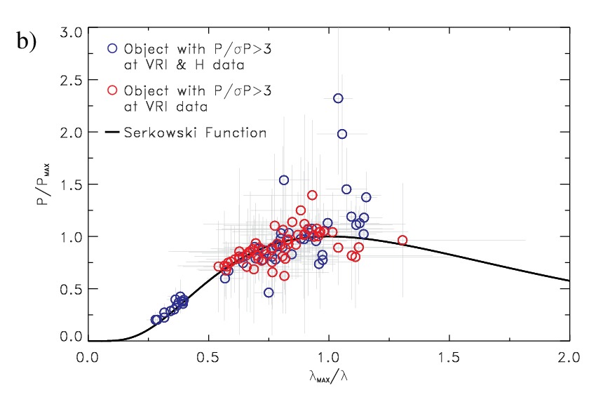
Figure 15.— (a): Example of the adjusted Serkowski relation ($P\times\lambda^{-1}$) and the wavelength dependence of polarization angle ($\theta\times\lambda^{-1}$) for a particular object presenting V, R, I and H data. The values of $P_{max}$, $\lambda_{max}$, $R_{V}$, and $\Delta\theta$ for this specific case are indicated at the top of the diagrams. (b): $(P/P_{max})\times(\lambda_{max}/\lambda)$ diagram, along with the Serkowski curve using points of all available bands for each of the 34 fitted objects. Stars with VRIH or VRI data are distinguished respectively by blue or red open circles.

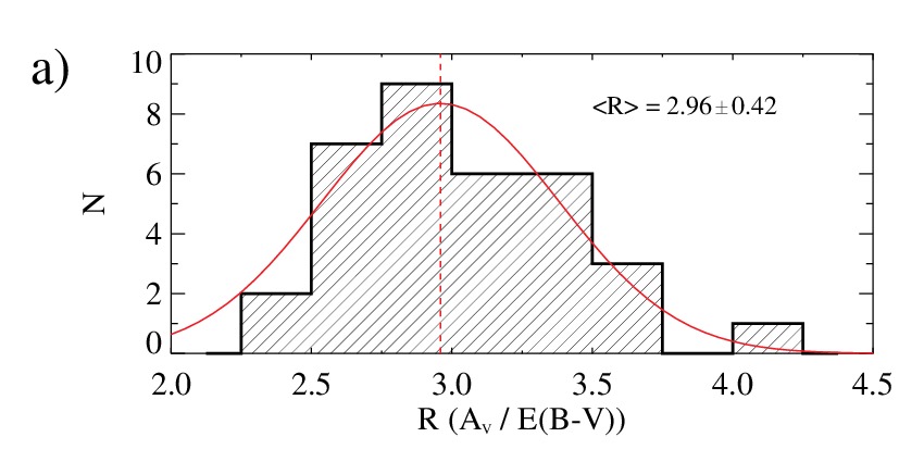
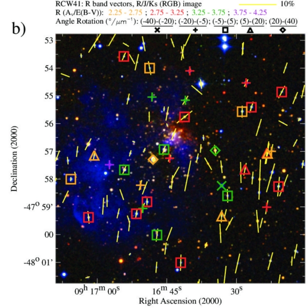
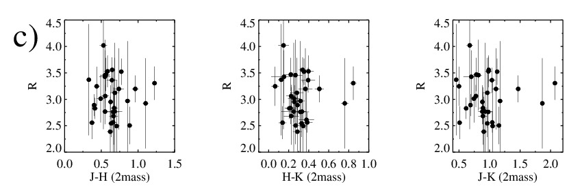
Figure 16.— (a): Distribution of the fitted values of the total-to-selective extinction ratio (R), along with a Gaussian fit indicating a mean R value of $\overline{R}=2.96\pm 0.42$. (b): Spatial distribution of the stars studied with the multi-band polarization data (represented by the colored symbols), along with the R-band polarization vectors, both overlaid in a R/J/Ks combined image of the RCW41 region. Symbols denote different angle rotation ($\Delta\theta$) intervals, and different colors represent different strips of the R value, as specified by the caption above the image. (c): Diagram of the obtained R values as a function of the NIR colors, showing no particular trend or concentration toward lower or higher values.

Figure 17.— H band polarization vectors map of an area of approximately $3.5^{\prime}\times 7.0^{\prime}$ encompassing the RCW41 stellar cluster. The image is a RGB combination of the H and Ks images from the SofI’s Dataset B NIR survey (respectively blue and green), and the $5.8\mu$m image from Spitzer’s IRAC (red), showing several filaments bended toward the cluster. Blue vectors, yellow vectors and green open circles respectively represent data with $P/\sigma_{P}>3$ (good quality), $3>P/\sigma_{P}>1$ (lower quality) and $P/\sigma_{P}<1$ (also indicating bad polarization data). Stars marked with open purple squares are possible contaminating field objects, presenting the following photometric features: $H-K\!s<0.5$ and $H>13.5$. Histograms denote the distribution of polarization angles for objects within each of the white dotted areas labeled as 1-6 (blue and yellow lines from the histograms also denote respectively good and lower quality data). The peak of each Gaussian fit is defined as the mean polarization orientation from that specific field. This mean angle is used to draw a grid inside each selected area, therefore denoting the mean local polarization orientation along that line-of-sight.

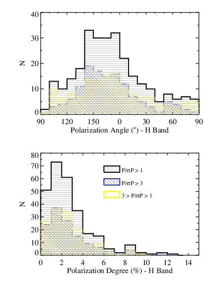
Figure 18.— Distributions of polarization angle (top) and polarization degree (bottom) for the NIR polarimetric survey in the H band. Blue lines are related to the data with $P/\sigma_{P}>3$ and yellow lines represent data with $3>P/\sigma_{P}>1$.

Figure 15b shows a diagram of $(P/P_{max})\times(\lambda_{max}/\lambda)$, where the individual $P_{max}$ and $\lambda_{max}$ fitted values were used together with the polarimetric data for the available bands. Red circles indicate polarimetric data to which the fitting was performed only with the VRI bands, while blue circles include also the H band. Note that, comparing the points with the position of the Serkowski curve, there is a larger dispersion toward lower $\lambda$ values (i.e., toward the V band). This is an expected effect since the signal-to-noise ratio of the polarimetric measurement for a particular embedded object is supposed to be smaller toward bluer colors. However, the overall fitted points forms a band around the Serkowski curve, therefore revealing a quite good adjustment.

We estimated the ratio of the total-to-selective extinction, $R_{V}$, by applying the well known relation between this parameter and $\lambda_{max}$ (Serkowski et al., 1975; Whittet & van Breda, 1978; Whittet, 2003),

$$R_{V}=(5.6\pm 0.3)\lambda_{max}$$ (3)

Figure 16a shows a histogram of the obtained $R_{V}$ values, indicating that most of them are concentrated between $\sim 2.5$ and $\sim 3.5$. By adjusting a Gaussian fit to this distribution, the peak value suggests a mean ratio of the total-to-selective extinction of $\overline{R}=2.96\pm 0.42$, which agrees with the standard value of $3.09$ for the typical interstellar grains. This finding gives support to the distance of $1.3\pm 0.2$ kpc for the embedded stellar cluster, obtained through spectroscopic techniques (Roman-Lopes et al., 2009). Furthermore, it also corroborates the position of the PMS isochrones and main sequence locus in the color-magnitude diagrams from the photometric analysis (Sections 3.4 and 3.5), since the standard interstellar law was assumed in those cases.

Figure 16b shows a R(DSS)/J/Ks(2MASS) composed image of the RCW41 region, with the local R-band polarization vectors distribution, and colored symbols indicating the objects from the multi-band analysis. Different colors for the symbols are related to different strips of $R_{V}$ values (divided in intervals of 0.5, as specified above the image), and the symbols indicate different intervals of the polarization angle rotation ($\Delta\theta$, where $\Box$ represent a small rotation level – between $-5$ and $5^{\circ}/\mu$m^-1 – while $\times$ and $\diamond$ denote high rotation levels respectively of $-40<\Delta\theta(^{\circ}/\mu$m${}^{-1})<-20$ and $20<\Delta\theta(^{\circ}/\mu$m${}^{-1})<40$).

Note that there is no spatial concentration of specific $R_{V}$ or $\Delta\theta$ values over the observed area. Although most of the $\Delta\theta$ values show low rotation levels, a great $\Delta\theta$ dispersion is found, with extreme high-rotation values of $-31$ and $37^{\circ}/\mu$m^-1. Along these directions, stellar light has probably passed through more than one interstellar layer with different grain alignment conditions. The $\Delta\theta$ dispersion is probably a consequence of a turbulent and fragmented medium associated to the Hii region, with superposing filaments depending on the chosen line-of-sight.

Figure 16c shows that there are no particular trend of the fitted $R_{V}$ values to any NIR color index. If stars with color excess due to circunstellar disks also show an intrinsic polarization level, this should interfere with the fits of the Serkowski relation, and therefore with the obtained $R_{V}$ values. However, these diagrams show no bias of the $R_{V}$ values toward higher color values.

4.5. The Small-scale Distribution of H-band Polarization Vectors

The H-band polarimetric survey is focused on the RCW41 cluster (Figure 4), and since most of the objects in this area are highly obscured in the visual wavelengths, the NIR survey provides a much larger number of polarization vectors at least in a region of a few parsecs around the star-forming locus.

Figure 17 shows the distribution of the H band polarization vectors surrounding the stellar cluster, superposed on a RGB combination of the H and Ks images (respectively blue and green, from SofI’s Dataset B), and the 5.8 $\mu$m image (red) collected using the Infrared Array Camera (IRAC) onboard Spitzer. The morphology of the mid-infrared extended emission is dominated by several conspicuous filaments emanating almost radially from the cluster. These structures resemble the pattern previously noted in the MSX 8.2 $\mu$m emission (Figure 11), but obviously with a much higher resolution, allowing the distinction of individual filaments near the cluster.

Polarization vectors are plotted with different colors according to the data quality (blue vectors have $P/\sigma_{P}>3$ while yellow vectors represent data with $3>P/\sigma_{P}>1$), and green circles denote lower quality polarization measurements. We have also adopted in this case a criteria to roughly separate contaminating field stars from cluster’s members, based on the fact that the polarimetric survey in the H band reaches an approximate photometric limit at $H=16$. We have found this information by correlating the polarimetric data with the photometric Dataset B and analyzing the H magnitudes distribution for the polarimetric sample. Therefore, by studying the color-magnitude diagram of Figure 7c, we notice that up to $H<16$, the contaminating stars are dominant if $H-K\!s\lesssim 0.5$ and $H\gtrsim 13.5$. Stars with such photometric characteristics are marked with a purple square in Figure 17, indicating that these are possibly field stars. A consistent trend in this diagram is that the number of field stars within the cluster is small, compared to the outer regions of the image, where this number increases.

The first striking evidence found in the distribution of polarimetric vectors is that the polarization angle dispersion is much larger than in the R band large-scale survey. This is probably an indication of the existence of a largely turbulent medium near the cluster. In fact, if we analyse the histogram of polarization angles for the entire H band sample (Figure 18, top panel), we can see that the entire range of possible angles is covered. However, a peak is reached at similar angles as in the large-scale distribution, i.e., at $\theta\sim 160^{\circ}$ suggesting that even in smaller scales, there is an underlying trend to follow the global scale pattern. Furthermore, no major differences are noted between the distributions of the good quality ($P/\sigma_{P}>3$, blue) and the low quality data ($3>P/\sigma_{P}>1$, yellow). The polarization degree distribution (Figure 18, bottom panel) shows that the majority of stellar objects present $P_{H}$ values within $1-4\%$.

Even when considering the large angle dispersion, we find that along even smaller regions within the area of Figure 17, some local trends may be unveiled, specially toward the interstellar filaments seen in $5.8\mu$m extended emission. In order to reveal these underlying features, we have selected six sub-areas, mainly encompassing the most prominent filaments, as indicated by the white dotted quadrangles marked with the 1-6 labels. Considering the polarization vectors within each of these areas, the associated histograms of polarization angles were built, being that objects marked as possible contaminating field stars were removed from the analysis. The distributions are also shown in Figure 17, linked to each respective area, and the division between good quality ($P/\sigma_{P}>3$) and low quality data ($3>P/\sigma_{P}>1$) are indicated respectively by the blue and yellow histograms. Gaussian fits were applied to each distribution, and the peak of the adjusted function corresponds to the main trend of the polarization angles within that area. By using this main value, a white dotted grid was drawn within each area, therefore corresponding to the local predominant polarimetric orientation.

We note that along the majority of the chosen areas, the main polarization direction seems to be consistent with the direction of the associated filament. Such trend is specially evident toward areas 2, 3 and 4. Specifically toward area 2, although only eight vectors contribute to the histogram, all of them are oriented parallel to the filament, presenting polarization angles around $\approx 110^{\circ}$. Such orientation is almost perpendicular to the main trend for the large-scale pattern, indicating a clear correlation with the local filament structure. Toward areas 1 and 6, a small difference seems to exist between the main polarization angle and the filament direction, although the orientation pointing in the direction of the cluster is evident. The existence of substructure or superposed filaments with different orientations along the line-of-sight may contribute to this displacement. Over area 5, which encompasses both the subcluster and a part of the main cluster region, an orientation pointing toward the cluster is also evident.

We conclude that despite the large angle dispersion, magnetic field lines on a small scale seem to be deflected inwards, pointing toward the cluster and probably connected to the direction of the large $5.8\mu$m filaments from the Spitzer survey. The polarization angle dispersion is indeed expected to exist in such a dynamical star forming region, where strong stellar winds from massive objects and possibly outflows from newborn lower mass stars, should play an important role as sources of turbulence to the surrounding interstellar medium. As a consequence, grain alignment efficiency and magnetic field lines are supposed to be affected, therefore characterizing a higher dispersion of the polarization orientations.

5. Discussion

5.1. Comparison of the magnetic field structure with theoretical studies on Hii regions’ expansion

Simulations conducted by Peters et al. (2010) describes the collapse of a massive molecular cloud followed by the formation of a small stellar cluster, which ionizes the accretion flow and causes the Hii region to expand. Spitzer (1978) first described the evolution of a photo-ionized region around an ionization source in a uniform medium, and provided an analytical solution to the expansion of the Hii region. However, several physical mechanisms, such as heating and cooling, turbulence, the effects of ionizing and non-ionizing ultraviolet radiation, X-rays, and magnetic fields, must be considered in order to provide a realistic view of the expansion process.

Arthur et al. (2011) have carried out simulations of this type considering the effects of a previously magnetized medium. Comparison of these simulations on non-magnetized and magnetized environments provide similar results in terms of the general morphology of the Hii regions, therefore suggesting that the presence of magnetic field lines does not cause a significant impact in providing resistance to the expansion of the ionized area, although this influence is most evident when considering the morphology of small-scale features, such as globules and interstellar filaments.

On the other hand, such expansion is expected to cause a large impact on the overall shape of the magnetic field lines. The main result from these simulations have shown that after the expansion of the Hii region, a dual behavior of the field’s morphology may be noticed when comparing the inside and outside regions of the ionized area: outside the Hii region (i.e., in the location of the neutral gas, following its borders), magnetic field lines tend to lie along the ionization front, forming a ring around the ionized area; inside the Hii region (i.e., within the ionized area), magnetic field lines are expected to lie perpendicular to the ionization front, therefore pointing towards the ionization source.

These qualitative predictions are consistent with the results of the large and small-scale polarimetric surveys of the RCW41 region introduced in Sections 4.1, 4.3, and 4.5. The R-band survey have revealed that magnetic field lines are bended along the borders of the Hii region toward some areas (Figures 11 and 14), which is consistent with the interpretation of magnetic field lines being pushed aside due to the expansion of the region, therefore lying along the ionization front on the neutral areas.

Moreover, our H-band polarimetric survey showed that, although a large angle dispersion is evident over the entire area, the mean polarization direction resembles a radially oriented field toward the cluster, roughly following the direction of several filaments from the mid-infrared Spitzer image. This is consistent with the theoretical prediction that inside the ionized area, field lines are expected to lie perpendicularly to the ionizing front. Assuming that the main ionizing sources in the region are Objects 1a and 2 (from Figure 6), as suggested by Ortiz et al. (2007) and Roman-Lopes et al. (2009), magnetic field lines should be pointing toward these targets, which is indeed obtained from the polarization vectors mean orientation (which points mainly toward Obj1a).

Such radial pattern is not noticed from the large-scale R-band map, although a large portion of this survey is composed by the ionized region, inside the Hii region. Furthermore, a perfect ring of polarimetric vectors is obviously not formed along the borders of the ionized area, as predicted by the simulations of the magnetic field lines. However, it is important to point out that the polarimetric survey is not a simple sky-projected slice of the Hii region. Rather, it represents the integrated effect of linear polarization due to different interstellar structures superposed along the line-of-sight. For example, if we imagine the Hii region roughly as an expanding sphere, such expansion will be noticed spatially in the sky, but will also occur in the line-of-sight direction. The expansion of the outer borders will push and pull interstellar material in our direction, causing the observations of the ionized region to be composed by the sky-projected, integrated polarizing effect due to the outer borders and the ionized region (if the observed star is located behind the Hii region). Therefore, the large-scale observations of the ionized region should account for this effect, and the radial pattern is not expected to be detected.

However, even when considering such effects, an indication of the dual behaviour of the polarimetric vectors’ orientation inside and outside the ionized area is certainly noticed when analysing the R-band and H-band polarization data. These observations give support to the results from the simulations, which provide similar qualitative predictions, at least when studying the specific environment of the RCW41 region.

5.2. The origin of the low polarization values within the Hii region

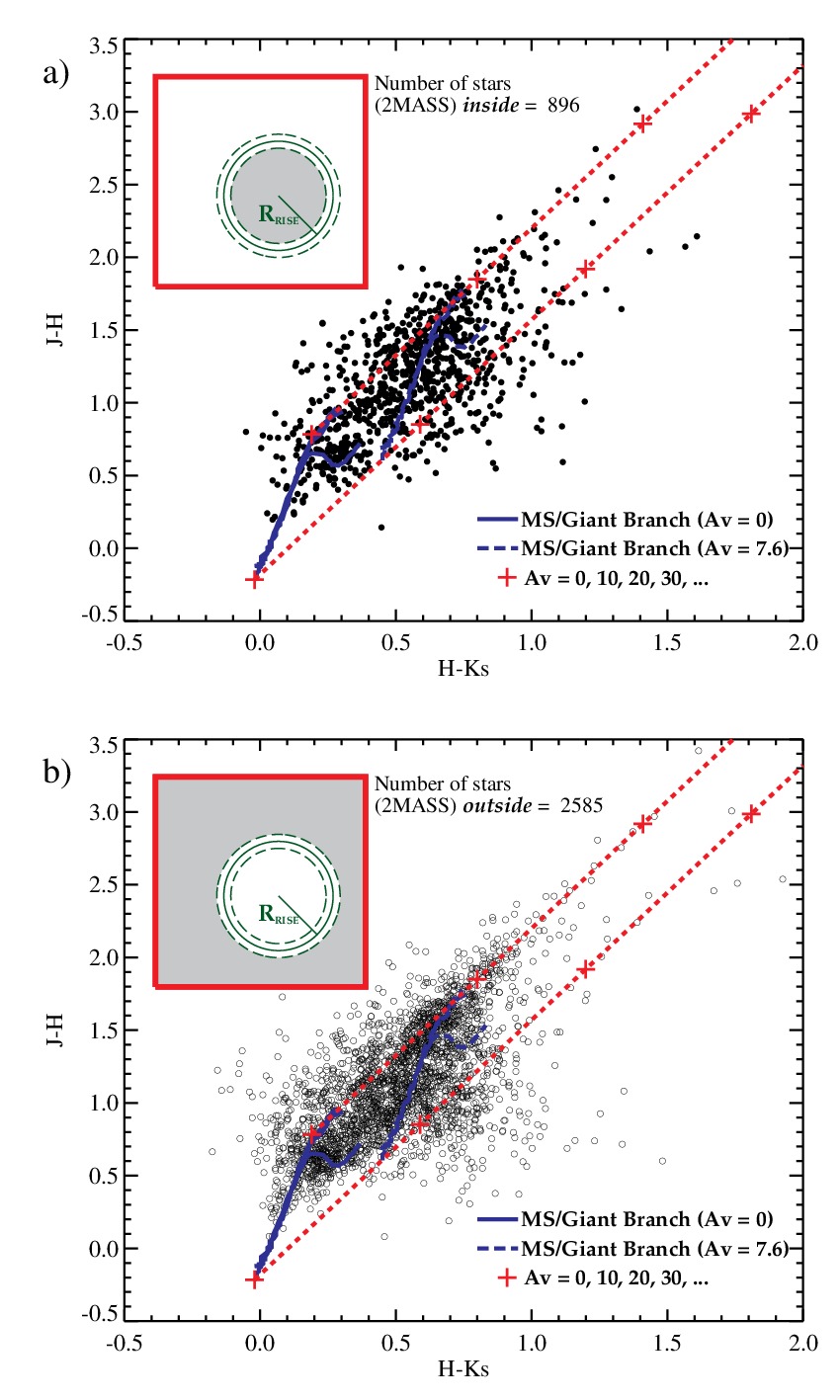
Figure 19.— $(J-H)\times(H-K\!s)$ (color-color) diagrams using data from 2MASS, for two separate regions along RCW41 (as indicated by the red boxes): inside (a) and outside (b) the Hii region. This area is defined as being delimited by the radius of $R_{rise}=7.8\pm 1.0$ arcmin from the center, where a sharp rise in R-band polarization degree is detected, as previously shown in Figure 14.

In Section 4.3 we have seen that an overall lower R-band polarization degrees are detected inside the Hii region, specially near the cluster.

In order to distinguish between the two possible mentioned causes responsible for such effect, two color-color diagrams have been built using 2MASS data, showing the distribution of stars inside (Figure 19a) and outside (Figure 19b) the limits defined by the sharp rise in polarization degree ($R_{rise}=7.8\pm 1.0$ arcmin), which roughly coincides with the limits of the Hii region. A larger number of stars is found outside the region, which is obviously due to the wider chosen area. However, when analyzing the distribution of stars along the reddening band (which gives an estimate of the interstellar extinction to each object), we notice that there are no major differences between both diagrams. In both areas, the majority of stars show a roughly uniform distribution of extinction values between $A_{V}=0$ and $A_{V}\approx 12$. Besides, we know that some concentrations mainly near the cluster (which comprises only a small area within the Hii region) may present larger mean local $A_{V}$ values (as discussed in Section 3.3). This analysis shows that no global decrease in interstellar extinction is detected inside the area.

Therefore, it seems that the observed decrease in polarization degree inside the Hii region is probably caused by a lower polarization efficiency of the local interstellar medium. This may be explained by an intrinsic suppression of the alignment of dust grains with respect to the interweaving magnetic field lines, which is expected given the dynamical and turbulent conditions of such interstellar environment.

Furthermore, in the simulations performed by Arthur et al. (2011), it was shown that the intensity of magnetic fields in the photo-ionized area is lower ($B=0.1-10\mu$G), when compared with the neutral areas from the border of the Hii region ($B=10-30\mu$G). This is probably explained due to the fact that the expansion of the ionized region causes the magnetic field lines to be pushed aside and therefore removed from inside the area, weakening the magnetic field in this location. If this is the scenario occurring in RCW41, a further depletion of polarization efficiency would be expected, contributing to the lower $P$ values detected near the cluster.

5.3. The turbulent component of the magnetic field toward RCW41

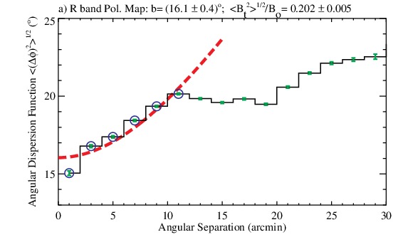
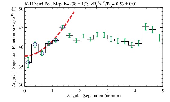
Figure 20.— Angular dispersion functions (ADF) constructed by using the polarization angles from the R band (a) and the H band (b) polarimetric datasets. Each bin (respectively of widths 2 and 0.25 arcmin) have already been corrected due to the mean measurement uncertainties. The red dashed line denote the curve obtained through the linear fit of the SF, by using the first six points on each case (blue circles). The turbulent contribution $b$ is determined by the interception of this curve at $l=0$, being subsequently used to compute the ratio of the turbulent to the large-scale magnetic field strength, which are shown at the top of each diagram.

The polarimetric dataset toward RCW41 is entirely suitable to apply a method which aims on estimating the turbulent contribution to the magnetic field lines, relative to its uniform component (Hildebrand et al., 2009). It is based on the assumption that the interstellar magnetic field $\mathbf{B}(\mathbf{x})$ is composed of a large-scale structured field $\mathbf{B_{0}}(\mathbf{x})$, together with a turbulent component $\mathbf{B_{t}}(\mathbf{x})$. Initially, the procedure consists basically in computing the second-order structure function of the polarization angles ($\langle\Delta\Phi^{2}(l)\rangle$, hereafter SF), which is defined as the average value of the squared difference in polarization angles between two points separated by a distance $l$ (see Equation (5) given by Falceta-Gonçalves et al., 2008). The square root of this quantity is denominated angular dispersion function (ADF), and provides information on the dispersion of polarization angles as a function of the length scale toward a specific interstellar area.

Hildebrand et al. (2009) pointed out that within the range $\delta<l\ll d$ (where $\delta$ and $d$ are the correlation lengths respectively characterizing $\mathbf{B_{t}}(\mathbf{x})$ and $\mathbf{B_{0}}(\mathbf{x})$), the SF is composed by: a constant turbulent contribution (denoted by $b$); a smoothly increasing contribution with respect to the length $l$, as expected from the uniform field (the slope of this linear behaviour is represented by $m$); and an almost constant contribution due to measurement uncertainties ($\sigma(l)$). Being statistically independent, these factors must be added quadratically, leading to

$$\langle\Delta\Phi^{2}(l)\rangle\simeq b^{2}+m^{2}l^{2}+\sigma^{2}(l)$$ (4)

The ratio of the turbulent to large-scale magnetic field strength is related to the quantity $b$ through the following expression:

$$\frac{\langle B_{t}^{2}\rangle^{1/2}}{B_{0}}=\frac{b}{\sqrt{2-b^{2}}}$$ (5)

Therefore, by constructing the SF (and computing the measurement uncertainties $\sigma(l)$) using the polarization angles, it is straightforward to apply a linear fit with Equation 4 and determine the $b$ factor (by the intercept at $l=0$).

Using the polarization angles from the R and H polarimetric datasets, we have computed the SF, as well as the mean measurement uncertainties $\sigma(l)$. Thereafter, the ADF was built to each case, as shown in Figures 20a and 20b, which are respectively related to the R and H band polarization data. Prior to calculating the ADF, the factor $\sigma^{2}(l)$ was subtracted within each bin of the SF, as suggested in Equation 4 (therefore, the value of each bin in Figure 20 is $\sqrt{\langle\Delta\Phi^{2}(l)\rangle-\sigma^{2}(l)}$). In diagrams 20a and 20b, bin widths of respectively $2$ and $0.25$ arcmin have been used. Only the first six points of the ADF (denoted by blue open circles) are used in the linear fit of Equation 4, in order to guarantee the validity of the $l\ll d$ regime, and the fitted function is represented by the red dashed line. The ratio of the turbulent to large-scale magnetic field strength was computed through Equation 5, resulting in $\langle B_{t}^{2}\rangle^{1/2}/B_{0}=(20.2\pm 0.5)\%$ and $\langle B_{t}^{2}\rangle^{1/2}/B_{0}=(53\pm 1)\%$ for the R and H band datasets, respectively.

The calculation shows that the turbulent component of the magnetic field is much stronger within the small scale area surrounding the cluster (i.e., where the H band data is distributed), when compared with the global turbulent contribution considering the entire area surrounding the Hii region (the R band data distribution). In fact, a higher turbulence ambient is expected to exist nearer the cluster due to the larger interaction between the young stars and the interstellar medium within this area. We may also associate this evidence with our hypothesis that the low polarization values inside the Hii region (mainly near the cluster, as seen in Figure 14b), indeed occurs due to low polarization efficiency. The higher turbulence level probably represents the main factor inhibiting the alignment of dust grains with respect to the magnetic field lines, causing the lower polarization values.

6. Conclusions

Using two sets of NIR photometric data collected using the SofI camera at the NTT 3.5 m telescope, we have characterized the stellar population of a deeply embedded stellar cluster related to the RCW41 Hii region. Furthermore, through optical (V, R and I bands) and NIR polarimetric observations (H band), obtained respectively with similar polarimetric modules at the 0.9 m telescope on CTIO/Chile and the 1.6 m telescope on OPD/Brazil, we have built linear polarization maps of the star-forming area. Our main results from both techniques are listed below:

(i) Analysis of photometric colors of cluster’s stars in comparison with field stars shows that a number of the cluster’s objects present color excess, which is typically associated with circunstellar disks of young PMS stars. The cluster also presents several highly reddened objects ($A_{V}>20$ mag);

(ii) A mean visual extinction of $A_{V}=7.6\pm 2.0$ is estimated for the cluster’s objects, based on the location of the majority of the stars on the color-color diagram, which roughly defines a band parallel to the reddened locus of CTT stars. This is corroborated by an independent $A_{V}$ computation using MS stars from the cluster;

(iii) The morphology of the cluster is divided between a main portion and a sub-cluster. There seems to exist a correlation between the location of the highly obscured objects with the HNCO contours, which is mostly concentrated toward the north of the cluster’s main part. Therefore, these are probably highly embedded objects, and a local rising extinction gradient in the south-north direction is probably present near the cluster. This evidence supports the idea that the interstellar material surrounding Obj2 (a O9v star at the sub-cluster, presumably the most massive object in the field) have already been swept out, while near the main portion, gas and dust are still beginning to be affected, according to the HNCO contours;

(iv) The color-magnitude diagrams of the cluster’s stars show that the majority of the objects are displaced toward higher color values, indicating that these stars are mainly young objects, also presenting color excess and non-uniform interstellar extinction. Comparison with PMS isochrones provide a mean cluster age between $2.5$ and $5.0$ Myr. Stars from the turn-on region (more massive) are mostly concentrated near the subcluster, suggesting that this area has been formed earlier, subsequently triggering star formation at the main portion of the cluster. Results from item (iii) corroborate this hypothesis;

(v) The nature of some objects previously observed through NIR spectroscopy was reviewed. Obj1b, the close companion to the massive B0v central object, is highly reddened and presents spectroscopic features similar to T Tau Sb, being therefore a very young T Tauri star. Objects 3, 5, and 6 were previously identified as late-type field stars, although their position in the color-magnitude diagrams is consistent with the T Tauri classification. Examples have been found of young objects with similar spectral features. Specifically, Obj3 is highly reddened ($A_{V}>20$) and very luminous, with spectral features that may be consistent with a medium mass YSO. Its weak CO absorption lines may be explained due to veiling from the circunstellar dust emission;

(vi) Using the density distribution of stars in the field, the cluster’s center has been determined to be at ($\alpha_{\mathrm{c}}$,$\delta_{\mathrm{c}}$)₂₀₀₀=($9^{\mathrm{h}}16^{\mathrm{m}}43.5^{\mathrm{s}}$,$-47^{\circ}56^{\prime}24.2^{\prime\prime}$). A two-parameter King function has been adjusted to the radial density profile, considering both the entire area around the cluster and a second fit where the portion encompassing the sub-cluster was removed, providing a much sharper profile. The general morphology shows that although some stellar scattering exist toward the south, the main cluster is probably of the centrally condensed-type. This shape is correlated to the spherical and similarly sized cloud core in which the cluster is immersed, as observed from the 1.2mm dust continuum emission toward RCW41.

(vii) The R-band polarimetric survey of a large area encompassing the entire Hii region, was used to build images of mean polarization degree and position angle. A radial analysis starting from the center of the ionized area revealed a sharp increase in polarization degree roughly coinciding with a conspicuous interstellar ring detected at the MSX 8.2$\mu$m emission, which delimits the ionized area. This evidence reflects a global decrease in polarization degree inside the Hii region, mainly near the cluster, which is most probably due to low grain alignment efficiency caused by the turbulent environment and weak magnetic fields in this area;

(viii) The image of mean polarization angle exhibit large areas, mainly toward the southwest of RCW41, where polarization angles are slanted outwards, following the borders of the ionized area. Such slanting coincides with the limits of the region indicated by the MSX 8.2$\mu$m emission, and is supported by simulations of the expansion of Hii regions, which predicts that the magnetic field lines at the neutral gas outside the limits of the region, tends to lie parallel to the ionization front;

(ix) The H-band polarimetric survey, focused on a smaller area towards the cluster, shows that, although a large dispersion of polarization angles are present, a mean pattern may be noticed: polarization vectors roughly follow the direction of several interstellar filaments, emanating radially from the cluster, as revealed by the Spitzer $5.8\mu$m image. Therefore, the mean orientation is roughly perpendicular to the ionization front, a result which is also in agreement with the predicted morphology of the magnetic field lines inside the ionized area, from simulations of expanding Hii regions;

(x) By combining polarimetric optical data (V, R, and I) and the NIR H-band, the Serkowski function has been fitted towards several stars mainly near the cluster. A large rotation of polarization angles is noticed toward some stars, revealing that the light beam has probably trespassed different interstellar layers along the line-of-sight. The total-to-selective extinction ratio has been computed toward each of the fitted objects, and a mean value of $\overline{R}=2.96\pm 0.42$ has been obtained, which agrees with the standard $3.09$ value for the typical interstellar medium extinction law.

(xi) Through the statistical correlation analysis (computing the ADFs using the R and H band polarimetric datasets), we have shown that the ratio of the turbulent to large-scale magnetic field strength is $(20.2\pm 0.5)\%$ when the entire area surrounding the Hii region is considered, and $(53\pm 1)\%$ if only the area near the cluster is taken into account. The higher turbulence level within the cluster area reinforces the hypothesis that the low polarization values at this region occurs due to the lower polarization efficiency.

Appendix A Photometric and Polarimetric Data

The lists related to the photometric data are available in Tables 1 (Dataset A) and 2 (Datset B), and the complete multi-band polarimetric sample is provided in Table 3. Tables 1, 2 and 3 are published in its entirety in the electronic edition of the Astrophysical Journal. A portion of each table is shown here for guidance regarding its form and content.

Table 1 NIR phtometric data of RCW41 from Dataset A.

$\alpha_{2000}(^{hms})$	$\delta_{2000}(\arcdeg\arcmin\arcsec)$	$J$	$\Delta J$	$H$	$\Delta H$	$K\!s$	$\Delta K\!s$
9 16 47.94	-47 57 17.8	9.712	0.022	8.962	0.015	8.653	0.026
9 17 1.91	-47 56 44.7	10.999	0.020	9.456	0.018	8.786	0.016
9 16 43.49	-47 56 22.9	10.684	0.021	9.865	0.015	9.492	0.026
9 17 4.34	-47 55 49.5	12.801	0.020	10.852	0.018	9.959	0.016
9 16 47.67	-47 57 21.2	12.037	0.022	10.910	0.015	10.486	0.026
9 16 41.89	-47 56 15.4	14.555	0.038	12.041	0.015	10.627	0.026
9 16 47.05	-47 56 44.0	12.636	0.021	11.481	0.015	11.039	0.026
9 17 8.72	-47 57 16.1	12.982	0.020	11.764	0.019	11.183	0.016
9 16 45.57	-47 56 56.0	12.387	0.021	11.707	0.015	11.391	0.026
9 16 44.89	-47 55 38.6	13.740	0.021	12.407	0.015	11.483	0.026

Table 2 NIR phtometric data of RCW41 from Dataset B.

$\alpha_{2000}(^{hms})$	$\delta_{2000}(\arcdeg\arcmin\arcsec)$	$H$	$\Delta H$	$K\!s$	$\Delta K\!s$
9 16 47.95	-47 57 17.8	*	*	8.621	0.036
9 17 4.88	-47 54 4.8	10.411	0.016	9.534	0.028
9 16 43.49	-47 56 22.8	9.944	0.024	9.543	0.028
9 17 4.34	-47 55 49.4	10.870	0.024	9.995	0.026
9 16 47.68	-47 57 21.2	10.920	0.016	10.455	0.021
9 16 56.95	-47 58 23.5	11.194	0.015	10.500	0.016
9 16 41.88	-47 56 15.4	12.068	0.022	10.666	0.024
9 16 25.46	-47 59 30.9	11.337	0.014	10.765	0.011
9 16 34.57	-47 56 58.3	11.650	0.015	10.814	0.015
9 16 50.51	-47 53 16.6	11.093	0.035	10.924	0.029

Table 3 The V, R, I and H polarimetric data set.

$\alpha_{2000}(^{hms})$	$\delta_{2000}(\arcdeg\arcmin\arcsec)$	Band	$P(\%)$	$\sigma_{P}(\%)$	$\theta(^{\circ})$	$\sigma\theta(^{\circ})$
9 15 37.95	-48 1 24.9	R	2.70	0.44	144.6	4.7
9 15 41.72	-47 53 10.7	R	5.33	1.26	3.3	6.8
9 15 43.66	-47 47 39.1	R	10.62	1.86	1.8	5.0
9 16 22.63	-47 57 57.1	V	10.47	3.34	171.1	9.1
		R	7.97	1.44	163.9	5.2
		I	6.12	0.99	162.1	4.6
9 16 25.00	-47 58 1.0	R	10.72	1.76	177.8	4.7
		I	7.32	0.75	0.1	3.0
9 16 36.83	-47 56 27.8	H	12.06	1.59	111.5	6.3
9 16 38.41	-47 57 14.9	V	3.16	0.31	167.7	2.9
		R	2.51	0.28	168.5	3.2
		I	2.86	0.35	174.1	3.5
		H	0.87	0.07	177.8	5.5
9 16 40.99	-47 55 9.9	V	3.60	0.61	138.7	4.9
		R	2.76	0.16	148.0	1.7
		I	2.35	0.09	150.8	1.1
		H	1.03	0.07	155.4	5.3
9 16 42.57	-47 57 24.4	V	4.67	5.42	159.6	33.2
		R	**	**	**	**
		I	2.66	2.53	139.4	27.2
		H	3.99	1.09	165.4	9.3
9 16 44.28	-47 58 17.1	V	0.85	0.38	178.0	12.7
		R	0.78	0.37	173.6	13.7
		I	0.44	0.34	170.7	22.4
		H	**	**	**	**
9 16 45.47	-48 0 3.4	H	11.43	1.73	147.2	6.6

References

- Arthur et al. (2011) Arthur, S. J., Henney, W. J., Mellema, G., de Colle, F., & Vázquez-Semadeni, E. 2011, MNRAS, 414, 1747
- Axon & Ellis (1976) Axon, D. J. & Ellis, R. S. 1976, MNRAS, 177, 499
- Bonatto et al. (2004) Bonatto, C., Bica, E., & Girardi, L. 2004, A&A, 415, 571
- Braz & Epchtein (1983) Braz, M. A. & Epchtein, N. 1983, A&AS, 54, 167
- Carpenter (2001) Carpenter, J. M. 2001, AJ, 121, 2851
- Casali & Eiroa (1995) Casali, M. M. & Eiroa, C. 1995, Ap&SS, 224, 17
- Churchwell et al. (2006) Churchwell, E., Povich, M. S., Allen, D., et al. 2006, ApJ, 649, 759
- Churchwell et al. (2007) Churchwell, E., Watson, D. F., Povich, M. S., et al. 2007, ApJ, 670, 428
- Connelley & Greene (2010) Connelley, M. S. & Greene, T. P. 2010, AJ, 140, 1214
- Coyne (1974) Coyne, G. V. 1974, AJ, 79, 565
- Crutcher (2005) Crutcher, R. 2005, in The Magnetized Plasma in Galaxy Evolution, ed. K. T. Chyzy, K. Otmianowska-Mazur, M. Soida, & R.-J. Dettmar , 103–110
- Davis & Greenstein (1951) Davis, Jr., L. & Greenstein, J. L. 1951, ApJ, 114, 206
- Duchêne et al. (2002) Duchêne, G., Ghez, A. M., & McCabe, C. 2002, ApJ, 568, 771
- Falceta-Gonçalves et al. (2008) Falceta-Gonçalves, D., Lazarian, A., & Kowal, G. 2008, ApJ, 679, 537
- Gehrels & Silvester (1965) Gehrels, T. & Silvester, A. B. 1965, AJ, 70, 579
- Girart et al. (2009) Girart, J. M., Beltrán, M. T., Zhang, Q., Rao, R., & Estalella, R. 2009, Science, 324, 1408
- Heiles & Crutcher (2005) Heiles, C. & Crutcher, R. 2005, in Lecture Notes in Physics, Berlin Springer Verlag, Vol. 664, Cosmic Magnetic Fields, ed. R. Wielebinski & R. Beck, 137
- Heitsch et al. (2004) Heitsch, F., Zweibel, E. G., Slyz, A. D., & Devriendt, J. E. G. 2004, ApJ, 603, 165
- Hildebrand et al. (2009) Hildebrand, R. H., Kirby, L., Dotson, J. L., Houde, M., & Vaillancourt, J. E. 2009, ApJ, 696, 567
- King (1962) King, I. 1962, AJ, 67, 471
- King (1966) King, I. R. 1966, AJ, 71, 276
- Koornneef (1983) Koornneef, J. 1983, A&A, 128, 84
- Krumholz et al. (2007) Krumholz, M. R., Stone, J. M., & Gardiner, T. A. 2007, ApJ, 671, 518
- Lada (2010) Lada, C. J. 2010, Royal Society of London Philosophical Transactions Series A, 368, 713
- Lada & Lada (2003) Lada, C. J. & Lada, E. A. 2003, ARA&A, 41, 57
- Liseau et al. (1992) Liseau, R., Lorenzetti, D., Nisini, B., Spinoglio, L., & Moneti, A. 1992, A&A, 265, 577
- Lizano & Shu (1989) Lizano, S. & Shu, F. H. 1989, ApJ, 342, 834
- Lorenzetti et al. (1993) Lorenzetti, D., Spinoglio, L., & Liseau, R. 1993, A&A, 275, 489
- Magalhaes et al. (1996) Magalhaes, A. M., Rodrigues, C. V., Margoniner, V. E., Pereyra, A., & Heathcote, S. 1996, in Astronomical Society of the Pacific Conference Series, Vol. 97, Polarimetry of the Interstellar Medium, ed. W. G. Roberge & D. C. B. Whittet, 118
- Massi et al. (1999) Massi, F., Giannini, T., Lorenzetti, D., et al. 1999, A&AS, 136, 471
- Massi et al. (2003) Massi, F., Lorenzetti, D., & Giannini, T. 2003, A&A, 399, 147
- Massi et al. (2000) Massi, F., Lorenzetti, D., Giannini, T., & Vitali, F. 2000, A&A, 353, 598
- Mathewson & Ford (1970) Mathewson, D. S. & Ford, V. L. 1970, MmRAS, 74, 139
- Matthews et al. (2002) Matthews, B. C., Fiege, J. D., & Moriarty-Schieven, G. 2002, ApJ, 569, 304
- McKee & Ostriker (2007) McKee, C. F. & Ostriker, E. C. 2007, ARA&A, 45, 565
- Messinger et al. (1997) Messinger, D. W., Whittet, D. C. B., & Roberge, W. G. 1997, ApJ, 487, 314
- Mestel & Spitzer (1956) Mestel, L. & Spitzer, Jr., L. 1956, MNRAS, 116, 503
- Meyer et al. (1997) Meyer, M. R., Calvet, N., & Hillenbrand, L. A. 1997, AJ, 114, 288
- Moorwood et al. (1998) Moorwood, A., Cuby, J.-G., & Lidman, C. 1998, The Messenger, 91, 9
- Mouschovias & Paleologou (1981) Mouschovias, T. C. & Paleologou, E. V. 1981, ApJ, 246, 48
- Murphy & May (1991) Murphy, D. C. & May, J. 1991, A&A, 247, 202
- Nakano (1979) Nakano, T. 1979, PASJ, 31, 697
- Olmi et al. (2009) Olmi, L., Ade, P. A. R., Anglés-Alcázar, D., et al. 2009, ApJ, 707, 1836
- Ortiz et al. (2007) Ortiz, R., Roman-Lopes, A., & Abraham, Z. 2007, A&A, 461, 949
- Padoan et al. (2004) Padoan, P., Jimenez, R., Juvela, M., & Nordlund, Å. 2004, ApJ, 604, L49
- Pereyra (2000) Pereyra, A. 2000, Ph.D. Thesis, Univ. São Paulo (Brazil)
- Peters et al. (2011) Peters, T., Banerjee, R., Klessen, R. S., & Mac Low, M.-M. 2011, ApJ, 729, 72
- Peters et al. (2010) Peters, T., Banerjee, R., Klessen, R. S., et al. 2010, ApJ, 711, 1017
- Pirogov et al. (2007) Pirogov, L., Zinchenko, I., Caselli, P., & Johansson, L. E. B. 2007, A&A, 461, 523
- Pirogov (2009) Pirogov, L. E. 2009, Astronomy Reports, 53, 1127
- Rieke & Lebofsky (1985) Rieke, G. H. & Lebofsky, M. J. 1985, ApJ, 288, 618
- Roman-Lopes et al. (2009) Roman-Lopes, A., Abraham, Z., Ortiz, R., & Rodriguez-Ardila, A. 2009, MNRAS, 394, 467
- Santos et al. (2011) Santos, F. P., Corradi, W., & Reis, W. 2011, ApJ, 728, 104
- Serkowski et al. (1975) Serkowski, K., Mathewson, D. L., & Ford, V. L. 1975, ApJ, 196, 261
- Shu et al. (1987) Shu, F. H., Adams, F. C., & Lizano, S. 1987, ARA&A, 25, 23
- Siess et al. (2000) Siess, L., Dufour, E., & Forestini, M. 2000, A&A, 358, 593
- Skrutskie et al. (2006) Skrutskie, M. F., Cutri, R. M., Stiening, R., et al. 2006, AJ, 131, 1163
- Spitzer (1978) Spitzer, L. 1978, Physical processes in the interstellar medium (New York Wiley-Interscience, 1978. 333 p.)
- Stetson (1987) Stetson, P. B. 1987, PASP, 99, 191
- Tang et al. (2009) Tang, Y.-W., Ho, P. T. P., Girart, J. M., et al. 2009, ApJ, 695, 1399
- Tapia (1988) Tapia, S. 1988, Preprints of the Steward Observatory, No. 831
- Tody (1986) Tody, D. 1986, Proc. SPIE, 627, 733
- Turnshek et al. (1990) Turnshek, D. A., Bohlin, R. C., Williamson, R. L., et al. 1990, AJ, 99, 1243
- Whittet (2003) Whittet, D. C. B. 2003, Dust in the galactic environment, 2nd ed (IoP Publishing, Bristol)
- Whittet et al. (1992) Whittet, D. C. B., Martin, P. G., Hough, J. H., et al. 1992, ApJ, 386, 562
- Whittet & van Breda (1978) Whittet, D. C. B. & van Breda, I. G. 1978, A&A, 66, 57
- Wilking et al. (1980) Wilking, B. A., Lebofsky, M. J., Kemp, J. C., Martin, P. G., & Rieke, G. H. 1980, ApJ, 235, 905
- Wilking et al. (1982) Wilking, B. A., Lebofsky, M. J., & Rieke, G. H. 1982, AJ, 87, 695
- Zinchenko et al. (2000) Zinchenko, I., Henkel, C., & Mao, R. Q. 2000, A&A, 361, 1079
- Zinchenko et al. (1995) Zinchenko, I., Mattila, K., & Toriseva, M. 1995, A&AS, 111, 95